A discontinuous Galerkin / cohesive zone model approach
for the computational modeling of fracture
in geometrically exact slender beams

Abstract

Slender beams are often employed as constituents in engineering materials and structures. Prior experiments on lattices of slender beams have highlighted their complex failure response, where the interplay between buckling and fracture plays a critical role. In this paper, we introduce a novel computational approach for modeling fracture in slender beams subjected to large deformations. We adopt a state-of-the-art geometrically exact Kirchhoff beam formulation to describe the finite deformations of beams in three-dimensions. We develop a discontinuous Galerkin finite element discretization of the beam governing equations, incorporating discontinuities in the position and tangent degrees of freedom at the inter-element boundaries of the finite elements. Before fracture initiation, we enforce compatibility of nodal positions and tangents weakly, via the exchange of variationally-consistent forces and moments at the interfaces between adjacent elements. At the onset of fracture, these forces and moments transition to cohesive laws modeling interface failure. We conduct a series of numerical tests to verify our computational framework against a set of benchmarks and we demonstrate its ability to capture the tensile and bending fracture modes in beams exhibiting large deformations. Finally, we present the validation of our framework against fracture experiments of dry spaghetti rods subjected to sudden relaxation of curvature.

[a]organization=Faculty of Aerospace Engineering, addressline=Delft University of Technology, state=2629 HS Delft, country=The Netherlands

[b]organization=Department of Materials Science and Engineering, addressline=Delft University of Technology, state=2628 CD Delft, country=The Netherlands

[c]organization=Delft Institute for Computational Science and Engineering, addressline=Delft University of Technology, state=2628 CD Delft, country=The Netherlands

1 Introduction

Slender beams are essential constituents of engineering materials and have a long history of serving as reinforcement elements in composite laminates [1], textiles [2], and paper products [3]. More recently, developments in additive manufacturing technology have enabled the combination of slender beams into engineered periodic truss lattices, giving rise to truss architected materials [4, 5]. In the wake of these technological advancements, there has been growing emphasis on designing optimal material microstructures capable of yielding specific target mechanical properties. For example, recent efforts within the scientific community have focused on designing material architectures aimed at achieving a desired anisotropic stiffness [6], optimal vibration control [7, 8], high specific stiffness and strength [9, 10, 11], and unprecedented specific impact energy absorption [12, 13]. While characterizing the failure modes of these materials is of paramount importance, particularly in the context of the performance-weight trade-off, the fracture mechanics of truss architected materials is not completely understood and remains an area of ongoing scientific interest.

Compression experiments on truss architected materials have highlighted the relevance of the interplay of buckling and fracture of the individual beam structural constituents in their overall failure response [9]. While buckling has been extensively studied in the literature in isolation, the interplay between buckling and fracture has traditionally received limited attention, perhaps due to the fact that buckling often leads to structural failure well before fracture initiation. More recently, as the structural engineering community has broadened its focus from developing buckling-safe structures to leveraging buckling instabilities as a design opportunity to create structures capable of adapting their shape to their surrounding environment [14, 15, 16], the study of the complex interplay between buckling and fracture in slender structures has gained increasing relevance.

Clearly, the complex fracture behavior of truss architected materials is significantly influenced by the combination of responses of the individual beam constituents. However, it is noteworthy that the buckling-to-fracture transition in a single slender beam already exhibits remarkable richness and complexity. A celebrated example is the fracture behavior of dry spaghetti rods, which consistently break into more than two pieces when subjected to large pure-bending stresses. This intriguing fracture behavior has puzzled numerous scientists, including the great physicist Richard Feynman [17]. Audoly and Neukirch later shed light on this phenomenon by uncovering a peculiar mechanical behavior of elastic rods in that the removal of stress leads to an increase in strain [18]. More specifically, the authors of that study theoretically predicted and confirmed through extensive experimentation that the sudden relaxation of curvature can trigger a burst of flexural waves, which locally increase the rod’s curvature, ultimately leading to cascading fragmentation.

While physical experiments are essential for understanding the fracture mechanics of slender beams, computational approaches offer complementary insights, especially in scenarios where experimental methods become impractical or where the efficient exploration of extensive parameter spaces is necessary. Preliminary research efforts aimed at developing computational models for fracture in beams can be found in the works of Armero and Ehrlich [19], Becker and Noels [20] and, more recently, Lai et al. [21]. These studies are based on Euler-Bernoulli beam theory but propose different approaches for fracture mechanics. Armero and Ehrlich [19] describe material failure via softening hinges modeled with the strong discontinuity approach. This approach, pioneered by Simo et al. [22], introduces discontinuities in the form of jumps of the solution field, which allow the characterization of the localized dissipative mechanisms associated with strain softening. Becker and Noels [20] adopt the discontinuous Galerkin / Cohesive Zone Model approach, originally introduced by Radovitzky et al. [23]. This computational fracture mechanics approach employs a discontinuous Galerkin discretization of the governing equations and models fracture as a process of decohesion across interfaces between finite elements. In contrast, Lai et al. [21] describe the fracture process via a phase-field model [24, 25]. Although these computational models have been successful in modeling failure in beams exhibiting small deformations, they cannot be used to model buckling-to-fracture transition, due to the infinitesimal-deformations assumption inherent in the underlying Euler-Bernoulli beam formulation. Likewise, beam fracture models that rely on Timoshenko beam theory, e.g. [26, 27, 28], are also unsuitable for capturing the transition from buckling to fracture.

Clearly, a fundamental requirement for a computational model for fracture of beams experiencing significant deformations is its foundation in a beam model able to accurately describe geometric nonlinearities . For example, Heisser et al. [30] found their beam fracture model on Kirchhoff beam theory, while Tojaga et al. [31] model fracture based on the finite-strain beam formulation by Simo [32]. More specifically, Heisser et al. [30] model the fragmentation of a beam by disconnecting adjacent elements instantaneously, upon satisfaction of a stress-based fracture criterion. However, this approach neglects the time-dependent aspects of the fracture process, which are known to be significant, particularly in the context of dynamic fragmentation [33, 34]. By contrast, Tojaga et al. [31] employ the strong discontinuity approach discussed above. In their work, the authors enrich the displacement field by introducing discontinuous modes at the elements midpoints. Beyond a critical load, they model failure at these discontinuities as a softening hinge. It is important to highlight that their approach models discontinuities exclusively in the displacement degrees of freedom, but not in the rotation degrees of freedom. As a consequence, their framework is capable of capturing fracture modes arising from tension and shear but not those resulting from bending.

In this paper, we present a computational framework to model fracture in slender beams subjected to finite deformations in three-dimensional space. We model the deformation of the beam with the geometrically exact Kirchhoff beam framework proposed by Meier et al. [35, 36]. Within this framework, we adopt the discontinuous Galerkin / Cohesive Zone Model approach for fracture mechanics. Following Meier et al. [35, 36], we approximate the beam’s deformation with the finite element method using third-order Hermitian polynomial shape functions. This choice is well-suited for the spatial discretization of beam formulations in view of the ability of Hermitian polynomials to meet the C¹ continuity compatibility requirement. However, instead of imposing compatibility strongly, we adopt a discontinuous Galerkin finite element approach and incorporate discontinuities in the position and tangent degrees of freedom at the inter-element boundaries of the finite elements. Before fracture initiation, we enforce compatibility of nodal positions and tangents weakly, via the exchange of variationally-consistent forces and moments at the interfaces between adjacent elements. At the onset of fracture, these variationally-consistent forces and moments transition to cohesive laws that model the fracture process. The finite element discretization described above results in a time-dependent algebraic system, which is solved in time with the second-order explicit Newmark scheme.

We conduct a series of numerical tests to verify our computational framework against a set of benchmarks and demonstrate its capability of accurately modeling tensile and bending fracture in slender beams exhibiting large deformations. First, we verify that the discontinuous Galerkin discretization is able to capture the analytical buckling load for a column. We then verify the discontinuous Galerkin / Cohesive Zone Model fracture mechanics approach in a bar spall fracture benchmark. Next, we show that the incorporation of discontinuities in the tangent degrees of freedom is essential for capturing the bending mode of fracture. Finally, we apply our computational framework to reproduce experiments by Audoly and Neukirch [18] on the fracture of dry spaghetti rods bent and suddenly released.

The structure of the paper is as follows. In Section 2, we briefly review the geometrically exact Kirchhoff beam formulation of [32, 35]. In Section 3, we derive the discontinuous Galerkin weak formulation of the beam governing equations and we propose a cohesive zone approach to describe fracture under tension and bending. We, then, outline the space and time discretization of the weak form and discuss our solution strategy for the discrete system of equations. We perform thorough verification and validation of the computational framework in Section 4. Conclusions are drawn in Section 5.

2 Geometrically exact Kirchhoff beam formulation

For completeness, we provide a concise summary of the geometrically exact beam governing equations by Simo [32] in their shear-free variant, as derived by Meier et al. [35]. We refer the reader to those two works for a more detailed and comprehensive discussion.

2.1 Kinematics

Following Simo [32], we characterize the beam configuration by the position of the beam centerline and by the orientation of its cross-sections. The centerline of the beam, i.e. the curve of the cross-sections centroids, is described with a suitable parametrization $\boldsymbol{r}(s)\in\mathbb{R}^{3}$, where $s\in[0,L]$ is the arc-length parameter, while the orientation of the beam cross-sections is described in terms of the orthonormal intrinsic frame $\{\boldsymbol{g_{1}}(s),\boldsymbol{g_{2}}(s),\boldsymbol{g_{3}}(s)\}$, see Figure 1. By convention, $\boldsymbol{g_{1}}(s)$ is chosen orthogonal to the beam cross-section at $s$, while $\boldsymbol{g_{2}}(s)$ and $\boldsymbol{g_{3}}(s)$ are chosen parallel to its principal axes of inertia. Note that, in general, $\boldsymbol{g_{1}}(s)$ is not tangent to the line of centroids $\boldsymbol{r}(s)$.

The deformed configuration of the beam can be expressed in terms of $\boldsymbol{r}$, $\boldsymbol{g_{2}}$, and $\boldsymbol{g_{3}}$ as:

$$\boldsymbol{x}(s,\xi_{2},\xi_{3})=\boldsymbol{r}(s)+\xi_{2}\ \boldsymbol{g_{2}}(s)+\xi_{3}\ \boldsymbol{g_{3}}(s),$$ (1)

where $\xi_{2}$ and $\xi_{3}$ are coordinates on the beam cross-section in the reference configuration.

For simplicity, it is often assumed that the beam is straight in its reference configuration, so that the intrinsic frame in the reference configuration can be chosen as a fixed basis $\{\boldsymbol{E_{1}},\boldsymbol{E_{2}},\boldsymbol{E_{3}}\}$ of $\mathbb{R}^{3}$. Because the vector basis $\{\boldsymbol{g_{i}}(s)\}$ is orthonormal at any cross-section $s$, there exists a rotation tensor $\boldsymbol{\Lambda}(s)$ such that:

$$\boldsymbol{g_{i}}(s)=\boldsymbol{\Lambda}(s)\boldsymbol{E_{i}},\quad i=1,2,3.$$ (2)

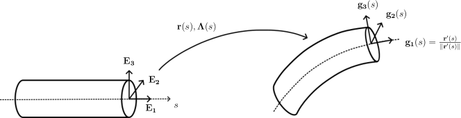
Figure 1: Illustration of the kinematics of a geometrically exact Kirchhoff beam in the case of a beam with circular cross-section. The beam configuration is characterized by the line of centroids $\boldsymbol{r}(s)$ and by the orthonormal intrinsic frame $\{\boldsymbol{g_{1}}(s),\boldsymbol{g_{2}}(s),\boldsymbol{g_{3}}(s)\}$. The Kirchhoff constraint enforces that $\boldsymbol{g_{1}}(s)$ be tangent to the line of centroids, that is $\boldsymbol{g_{1}}(s)=\frac{\boldsymbol{r}^{\prime}(s)}{||\boldsymbol{r}^{\prime}(s)||}$.

Kinematically admissible variations of $\boldsymbol{r}$ and $\boldsymbol{g_{i}}$ are denoted with $\boldsymbol{\delta r}$ and $\boldsymbol{\delta g_{i}}$, respectively. A direct consequence of Equation (2) is that kinematically admissible variations of $\boldsymbol{g_{i}}$ can be expressed as

$$\boldsymbol{\delta g_{i}}(s)=\boldsymbol{\delta\Lambda}(s)\boldsymbol{\Lambda^{T}}(s)\boldsymbol{g_{i}}(s).$$ (3)

Because tensor $\left(\boldsymbol{\delta\Lambda}\right)\boldsymbol{\Lambda^{T}}$ is skew-symmetric, Equation (3) can be rewritten as

$$\boldsymbol{\delta g_{i}}(s)=\boldsymbol{\delta\theta}(s)\times\boldsymbol{g_{i}}(s),$$ (4)

where $\boldsymbol{\delta\theta}$ is the axial vector of $\left(\boldsymbol{\delta\Lambda}\right)\boldsymbol{\Lambda^{T}}$. Under the hypothesis of negligible shear strains, which is a well-accepted assumption in the case of slender beams [35], $\boldsymbol{\delta\theta}$ is not independent of $\boldsymbol{\delta r}^{\prime}$. In fact, a relation between $\boldsymbol{\delta\theta}$ and $\boldsymbol{\delta r}^{\prime}$ can be obtained by kinematically enforcing that the beam centerline remain perpendicular to the cross-sections during the deformation (Kirchhoff constraint):

$$\boldsymbol{g_{1}}(s)=\frac{\boldsymbol{r}^{\prime}(s)}{||\boldsymbol{r}^{\prime}(s)||},$$ (5)

where $(\cdot)^{\prime}$ denotes the derivative with respect to the arc-length parameter. Plugging Equation (5) into Equation (4), we obtain the following relation:

$$\boldsymbol{\delta\theta}(s)=\frac{\boldsymbol{r}^{\prime}(s)\times\boldsymbol{\delta r}^{\prime}(s)}{||\boldsymbol{r}^{\prime}(s)||^{2}}+\frac{\boldsymbol{r}^{\prime}(s)}{||\boldsymbol{r}^{\prime}(s)||}\delta\alpha,$$

prescribing the kinematically admissible variations of rotations $\boldsymbol{\delta\theta}$ in terms of the kinematically admissible variations of the centerline tangents $\boldsymbol{\delta r}^{\prime}$ and of the beam torsion

$$\delta\alpha(s):=\boldsymbol{\delta\theta}(s)\cdot\frac{\boldsymbol{r}^{\prime}(s)}{||\boldsymbol{r}^{\prime}(s)||}.$$

In this work, we limit our attention to the simpler torsion-free case ($\delta\alpha=0$), so that:

$$\boldsymbol{\delta\theta}(s)=\boldsymbol{\delta\theta}_{\perp}(s):=\frac{\boldsymbol{r}^{\prime}(s)\times\boldsymbol{\delta r}^{\prime}(s)}{||\boldsymbol{r}^{\prime}(s)||^{2}}.$$ (6)

2.2 Balance of linear and angular momentum

The governing equations of the beam can be derived by integrating the linear and angular momentum balance equations from the 3D continuum theory over the cross-section of the beam. We refer the reader to Simo [32] for a detailed derivation, while we report here only the final expressions:

$$\boldsymbol{f}^{\prime}+\boldsymbol{\tilde{f}}=\rho A\boldsymbol{\ddot{r}},$$ (7)

$$\boldsymbol{m}^{\prime}+\boldsymbol{r}^{\prime}\times\boldsymbol{f}+\boldsymbol{\tilde{m}}=\boldsymbol{I_{\rho}}\boldsymbol{\dot{\omega}}+\boldsymbol{\omega\times(I_{\rho}\omega)}.$$ (8)

Here, the prime and dot symbols denote arc-length and material time derivatives, respectively, while $\rho$, $A$, and $\boldsymbol{I_{\rho}}$ are the referential mass density, area of cross-section, and spatial inertia tensor of the beam. $\boldsymbol{\omega}$ is the axial vector corresponding to the the skew-symmetric angular velocity tensor $\dot{\boldsymbol{\Lambda}}\boldsymbol{\Lambda}^{T}$, while $\boldsymbol{f}(s,t)$ and $\boldsymbol{m}(s,t)$ are the internal force and moment stress resultants:

$$\boldsymbol{f}=\int_{A}\boldsymbol{P}\boldsymbol{E_{1}}\ \text{d}A,$$ (9)

$$\boldsymbol{m}=\int_{A}\left(\boldsymbol{x}-\boldsymbol{r}\right)\times\boldsymbol{P}\boldsymbol{E_{1}}\ \text{d}A,$$ (10)

where $\boldsymbol{P}$ is the Piola-Kirchhoff stress tensor. Finally, $\boldsymbol{\tilde{f}}$ and $\boldsymbol{\tilde{m}}$ are the external distributed forces and moments per unit referential arc-length.

Forces $\boldsymbol{f}$, $\boldsymbol{\tilde{f}}$ and moments $\boldsymbol{m}$, $\boldsymbol{\tilde{m}}$ can be additively decomposed into axial $\boldsymbol{f_{||}}$, $\boldsymbol{\tilde{f}_{||}}$ and shear $\boldsymbol{f_{\perp}}$, $\boldsymbol{\tilde{f}_{\perp}}$ forces, and bending $\boldsymbol{m_{\perp}}$, $\boldsymbol{\tilde{m}_{\perp}}$ and twisting $\boldsymbol{m_{||}}$, $\boldsymbol{\tilde{m}_{||}}$ moments, where

$$\boldsymbol{a_{||}}:=\left(\boldsymbol{a}\cdot\frac{\boldsymbol{r}^{\prime}}{||\boldsymbol{r}^{\prime}||}\right)\frac{\boldsymbol{r}^{\prime}}{||\boldsymbol{r}^{\prime}||},\qquad\boldsymbol{a_{\perp}}:=\boldsymbol{a}-\boldsymbol{a_{||}}.$$

Under the assumption that rotational inertia (i.e. the right-hand side of Equation (8)) can be neglected, which is a well-accepted assumption for the case of slender beams [37, 38], the following equation expressing the internal shear forces as a function of the bending moments can be obtained by performing the cross product of Equation (8) with $\boldsymbol{r}^{\prime}$:

$$\boldsymbol{f_{\perp}}=\frac{\boldsymbol{r}^{\prime}}{||\boldsymbol{r}^{\prime}||^{2}}\times\big{(}\boldsymbol{m_{\perp}}^{\prime}+\boldsymbol{\tilde{m}_{\perp}}\big{)}$$ (11)

Equation (11) can be plugged into Equation (7), leading to:

$$\boldsymbol{f_{||}}^{\prime}+\Bigg{[}\frac{\boldsymbol{r}^{\prime}}{||\boldsymbol{r}^{\prime}||^{2}}\times\big{(}\boldsymbol{m^{\prime}_{\perp}}+\boldsymbol{\tilde{m}_{\perp}}\big{)}\Bigg{]}^{\prime}+\boldsymbol{\tilde{f}}=\rho A\boldsymbol{\ddot{r}}.$$ (12)

Note that, when torsion is negligible, Equation (11) is equivalent to Equation (8). As a consequence, Equation (12) is equivalent to the original system of governing equations (7) and (8). In this work, we focus on the simpler torsion-free case and we use Equation (12) to model the finite deformations of the beam.

Equation (12) is complemented with suitable initial conditions for positions and tangents, and boundary conditions, in terms of applied forces and bending moments on the Neumann boundary or imposed positions and tangents on the Dirichlet boundary.

2.3 Constitutive equations

In this study, we confine our attention to isotropic beams with circular cross-sections. Assuming hyperelastic material behavior, the internal axial forces and bending moments are related to the axial strain $\epsilon=||\boldsymbol{r}^{\prime}||-1$ and the curvature $\boldsymbol{\kappa}=\frac{\boldsymbol{r}^{\prime}\times\boldsymbol{r^{\prime\prime}}}{||\boldsymbol{r}^{\prime}||^{2}}$ through the following constitutive relations [36]:

$$\boldsymbol{f_{||}}=EA\epsilon\frac{\boldsymbol{r}^{\prime}}{||\boldsymbol{r}^{\prime}||},\qquad\boldsymbol{m_{\perp}}=EI\boldsymbol{\kappa},$$ (13)

where $E$, $A$ and $I$ are the Young’s modulus, cross-sectional area and moment of inertia of the beam, respectively.

3 Computational framework for fracture in geometrically exact slender beams

In this section, we derive our discontinuous Galerkin / Cohesive Zone Model approach for fracture in geometrically exact slender beams. We first derive the discontinuous Galerkin weak formulation of the beam governing equations presented in Section 2. We, then, discuss the fracture modes of beams and propose cohesive laws to model the tensile and bending modes of beam fracture. Finally, we present the weak formulation of the discontinuous Galerkin / Cohesive Zone Model and we discuss its space and time discretization.

3.1 Derivation of the discontinuous Galerkin weak form

We consider a space discretization $\Omega_{h}$ of the straight undeformed beam $\Omega$ into segments $\Omega_{e}=(s_{0}^{e},s_{1}^{e})$, $e=1,...,E$, so that $\Omega_{h}=\bigcup\limits_{e=1}^{E}\overline{\Omega}_{e}$, see schematic in Figure 2. We denote with $\partial\Omega_{h}=\{0,L\}$ the boundary of the beam, whose external normal $n_{e}$ is $n_{e}=1$ at $s=L$ and $n_{e}=-1$ at $s=0$. Finally, we denote with $\partial_{N_{f}}\Omega_{h}$ and $\partial_{N_{m}}\Omega_{h}$ the Neumann portions of $\partial\Omega_{h}$, where we apply forces $\boldsymbol{\bar{f}}$ and moments $\boldsymbol{\bar{m}}_{\perp}$, respectively.

Figure 2: The discontinuous Galerkin discretization of the straight undeformed beam. Internal nodes, e.g. nodes $s_{1}^{e}$ and $s_{0}^{e+1}$, are duplicated to allow the embedding of potential discontinuities at the interfaces $s_{n}$ for $n=1,...,E-1$.

We consider Equation (12), where we allow $\boldsymbol{r}(s)$ and its associated kinematically admissible variations $\boldsymbol{\delta r}(s)$ to exhibit discontinuities at the interfaces $s_{n}$, $n=1,...,E-1$ of adjacent elements. We start the derivation of the discontinuous Galerkin weak form of Equation (12) by multiplying it with $\boldsymbol{\delta r}$, integrating over the individual subdomains $\Omega_{e}$, $e=1,...,E$, and performing the integration by parts:

$$-\sum_{e=1}^{E}\int_{\Omega_{e}}\boldsymbol{f_{||}}\cdot\boldsymbol{\delta r}^{\prime}\>ds -\sum_{e=1}^{E}\int_{\Omega_{e}}\boldsymbol{f_{\perp}}\cdot\boldsymbol{\delta r}^{\prime}\>ds-\sum_{n=1}^{E-1}\>[\![\boldsymbol{f}\cdot\boldsymbol{\delta r}]\!]\Big{|}_{s_{n}}+\left(\boldsymbol{\bar{f}}\cdot\boldsymbol{\delta r}\right)\Big{|}_{\partial_{N_{f}}\Omega_{h}}$$ (14)

$$+\sum_{e=1}^{E}\int_{\Omega_{e}}\boldsymbol{\tilde{f}}\cdot\boldsymbol{\delta r}\>ds=\sum_{e=1}^{E}\int_{\Omega_{e}}\rho A\boldsymbol{\ddot{r}}\cdot\boldsymbol{\delta r}\>ds,$$

where we have applied the Neumann boundary condition $\boldsymbol{\bar{f}}=n_{e}\boldsymbol{f}$ on $\partial_{N_{f}}\Omega_{h}$. In Equation (14), the notation $\bullet\Big{|}_{a}$ means $\bullet$ evaluated at $s=a$, while

$$[\![\bullet]\!]\Big{|}_{a}:=\lim_{s\rightarrow a^{+}}\bullet-\lim_{s\rightarrow a^{-}}\bullet$$

represents the jump of $\bullet$ at $s=a$. We also define the average of $\bullet$ at $s=a$ as

$$\langle{\bullet}\rangle\Big{|}_{a}:=\frac{1}{2}\left(\lim_{s\rightarrow a^{+}}\bullet+\lim_{s\rightarrow a^{-}}\bullet\right).$$

Using the identity $[\![\boldsymbol{a}\cdot\boldsymbol{b}]\!]=\langle\boldsymbol{a}\rangle\cdot[\![\boldsymbol{b}]\!]+[\![\boldsymbol{a}]\!]\cdot\langle\boldsymbol{b}\rangle$, we can rewrite the jump term in Equation (14) as:

$$\sum_{n=1}^{E-1}\>[\![\boldsymbol{f}\cdot\boldsymbol{\delta r}]\!]\Big{|}_{s_{n}}=\sum_{n=1}^{E-1}\>\Big{[}\langle\boldsymbol{f}\rangle\cdot[\![\boldsymbol{\delta r}]\!]\Big{]}\Big{|}_{s_{n}}+\sum_{n=1}^{E-1}\>\Big{[}[\![\boldsymbol{f}]\!]\cdot\langle\boldsymbol{\delta r}\rangle\Big{]}\Big{|}_{s_{n}}.$$ (15)

In addition, Equation (11), together with the vector identity $\boldsymbol{a}\cdot(\boldsymbol{b}\times\boldsymbol{c})=\boldsymbol{c}\cdot(\boldsymbol{a}\times\boldsymbol{b})$, allows us to rewrite the second term of Equation (14) as:

$$-\sum_{e=1}^{E}\int_{\Omega_{e}}\boldsymbol{f_{\perp}}\cdot\boldsymbol{\delta r}^{\prime}\>ds =\sum_{e=1}^{E}\int_{\Omega_{e}}\left(\boldsymbol{m_{\perp}}^{\prime}+\boldsymbol{\tilde{m}_{\perp}}\right)\cdot\frac{\boldsymbol{r}^{\prime}\times\boldsymbol{\delta r}^{\prime}}{||\boldsymbol{r}^{\prime}||^{2}}\>ds$$ (16)

$$=\sum_{e=1}^{E}\int_{\Omega_{e}}\left(\boldsymbol{m_{\perp}}^{\prime}+\boldsymbol{\tilde{m}_{\perp}}\right)\cdot\boldsymbol{\delta\theta}_{\perp}\>ds.$$

Note that the kinematically admissible variation $\boldsymbol{\delta\theta}_{\perp}$ of Equation (6) arises naturally as the work conjugate of the moments. In the following derivation, we will omit the subscript in $\boldsymbol{\delta\theta}_{\perp}$ and simply write $\boldsymbol{\delta\theta}$ for the sake of a lighter notation. The right-hand side of Equation (16) can be, in turn, integrated by parts, leading to:

$$\sum_{e=1}^{E}\int_{\Omega_{e}}\left(\boldsymbol{m_{\perp}}^{\prime}+\boldsymbol{\tilde{m}_{\perp}}\right)\cdot\boldsymbol{\delta\theta}\>ds=\sum_{e=1}^{E}\int_{\Omega_{e}}\boldsymbol{\tilde{m}_{\perp}}\cdot\boldsymbol{\delta\theta}\>ds-\sum_{e=1}^{E}\int_{\Omega_{e}}\boldsymbol{m_{\perp}}\cdot\boldsymbol{\delta\theta}^{\prime}\>ds$$ (17)

$$\qquad-\sum_{n=1}^{E-1}\>\Big{[}\langle\boldsymbol{m_{\perp}}\rangle\cdot[\![\boldsymbol{\delta\theta}]\!]\Big{]}\Big{|}_{s_{n}}-\sum_{n=1}^{E-1}\>\Big{[}[\![\boldsymbol{m_{\perp}}]\!]\cdot\langle\boldsymbol{\delta\theta}\rangle\Big{]}\Big{|}_{s_{n}}+\left(\boldsymbol{\bar{m}_{\perp}}\cdot\boldsymbol{\delta\theta}\right)\Big{|}_{\partial_{N_{m}}\Omega_{h}},$$

where we have applied the Neumann boundary condition $\boldsymbol{\bar{m}}_{\perp}=n_{e}\boldsymbol{m}_{\perp}$ on $\partial_{N_{m}}\Omega_{h}$ and used again the identity $[\![\boldsymbol{a}\cdot\boldsymbol{b}]\!]=\langle\boldsymbol{a}\rangle\cdot[\![\boldsymbol{b}]\!]+[\![\boldsymbol{a}]\!]\cdot\langle\boldsymbol{b}\rangle$.

Gathering Equations (14), (15), (16), and (17), we obtain:

$$\sum_{e=1}^{E}\int_{\Omega_{e}}\rho A\boldsymbol{\ddot{r}}\cdot\boldsymbol{\delta r}\>ds+\sum_{e=1}^{E}\int_{\Omega_{e}}\boldsymbol{f_{||}}\cdot\boldsymbol{\delta r}^{\prime}\>ds+\sum_{n=1}^{E-1}\>\Big{[}\langle\boldsymbol{f}\rangle\cdot[\![\boldsymbol{\delta r}]\!]\Big{]}\Big{|}_{s_{n}}+\sum_{n=1}^{E-1}\>\Big{[}[\![\boldsymbol{f}]\!]\cdot\langle\boldsymbol{\delta r}\rangle\Big{]}\Big{|}_{s_{n}}$$ (18)

$$+\sum_{e=1}^{E}\int_{\Omega_{e}}\boldsymbol{m_{\perp}}\cdot\boldsymbol{\delta\theta}^{\prime}\>ds+\sum_{n=1}^{E-1}\>\Big{[}\langle\boldsymbol{m_{\perp}}\rangle\cdot[\![\boldsymbol{\delta\theta}]\!]\Big{]}\Big{|}_{s_{n}}+\sum_{n=1}^{E-1}\>\Big{[}[\![\boldsymbol{m_{\perp}}]\!]\cdot\langle\boldsymbol{\delta\theta}\rangle\Big{]}\Big{|}_{s_{n}}$$

$$=\sum_{e=1}^{E}\int_{\Omega_{e}}\boldsymbol{\tilde{f}}\cdot\boldsymbol{\delta r}\>ds+\left(\boldsymbol{\bar{f}}\cdot\boldsymbol{\delta r}\right)\Big{|}_{\partial_{N_{f}}\Omega_{h}}+\sum_{e=1}^{E}\int_{\Omega_{e}}\boldsymbol{\tilde{m}_{\perp}}\cdot\boldsymbol{\delta\theta}\>ds+\left(\boldsymbol{\bar{m}_{\perp}}\cdot\boldsymbol{\delta\theta}\right)\Big{|}_{\partial_{N_{m}}\Omega_{h}}.$$

Since jumps in forces $\boldsymbol{f}$ and bending moments $\boldsymbol{m_{\perp}}$ need not be penalized to ensure the consistency of the numerical scheme, the terms involving their jumps in Equation (18) can be ignored, see also [39, 20]. However, the inter-element compatibility has to be enforced weakly to ensure the stability of the numerical scheme. Here, we do so through the interior penalty method, following [39, 20]. Specifically, we add the following terms to the left-hand side of Equation (18):

$$\sum_{n=1}^{E-1}\beta_{p}\Big{[}\bigg{\langle}\frac{EA}{h}\bigg{\rangle}[\![\boldsymbol{\delta r}]\!]\cdot[\![\boldsymbol{r}]\!]\Big{]}\Big{|}_{s_{n}}+\sum_{n=1}^{E-1}\beta_{t}\Big{[}\bigg{\langle}\frac{EI}{h}\bigg{\rangle}[\![\boldsymbol{\delta g_{1}}]\!]\cdot[\![\boldsymbol{g_{1}}]\!]\Big{]}\Big{|}_{s_{n}},$$

where we recall that $\boldsymbol{g_{1}}=\frac{\boldsymbol{r}^{\prime}}{||\boldsymbol{r}^{\prime}||}$ (see Equation (5)), while $\beta_{p}>1$ and $\beta_{t}>1$ are position and tangent jump penalty parameters and $h$ is the element size. We, therefore, obtain the following stabilized discontinuous Galerkin weak form:

$$\int_{\Omega_{h}}\rho A\boldsymbol{\ddot{r}}\cdot\boldsymbol{\delta r}\>ds +\int_{\Omega_{h}}EA\>\varepsilon\>\delta\varepsilon\>ds+\sum_{n=1}^{E-1}\>\Big{[}\langle\boldsymbol{f}\rangle\cdot[\![\boldsymbol{\delta r}]\!]\Big{]}\Big{|}_{s_{n}}+\sum_{n=1}^{E-1}\beta_{p}\Big{[}\bigg{\langle}\frac{EA}{h}\bigg{\rangle}[\![\boldsymbol{r}]\!]\cdot[\![\boldsymbol{\delta r}]\!]\Big{]}\Big{|}_{s_{n}}$$ (19)

$$+\int_{\Omega_{h}}EI\>\boldsymbol{\kappa}\cdot\boldsymbol{\delta\kappa}\>ds+\sum_{n=1}^{E-1}\>\Big{[}\langle\boldsymbol{m_{\perp}}\rangle\cdot[\![\boldsymbol{\delta\theta}]\!]\Big{]}\Big{|}_{s_{n}}+\sum_{n=1}^{E-1}\beta_{t}\Big{[}\bigg{\langle}\frac{EI}{h}\bigg{\rangle}[\![\boldsymbol{g_{1}}]\!]\cdot[\![\boldsymbol{\delta g_{1}}]\!]\Big{]}\Big{|}_{s_{n}}$$

$$=\int_{\Omega_{h}}\boldsymbol{\tilde{f}} \cdot\boldsymbol{\delta r}\>ds+\left(\boldsymbol{\bar{f}}\cdot\boldsymbol{\delta r}\right)\Big{|}_{\partial_{N_{f}}\Omega_{h}}+\int_{\Omega_{h}}\boldsymbol{\tilde{m}_{\perp}}\cdot\boldsymbol{\delta\theta}\>ds+\left(\boldsymbol{\bar{m}_{\perp}}\cdot\boldsymbol{\delta\theta}\right)\Big{|}_{\partial_{N_{m}}\Omega_{h}},$$

where we have also applied the constitutive relations (13).

3.2 Cohesive zone approach for fracture in beams

Beams exhibit several modes of fracture, which we illustrate in Figure 3. In fact, beams can fail under tensile, transverse, twisting or bending loads. However, in this work, we focus our attention on slender beams, which fail predominantly under tension and bending.

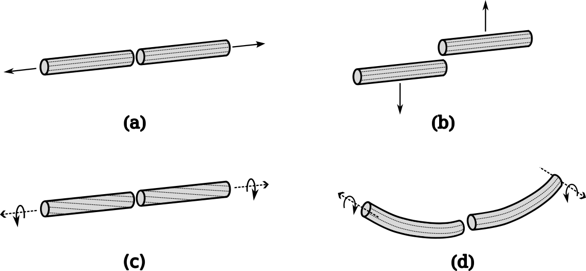
Figure 3: The fracture modes of beams: (a) tension, (b) transverse shear, (c) torsion and (d) bending.

We adopt the cohesive zone approach to model the beam fracture behavior. However, instead of employing the conventional traction-separation laws typical in cohesive zone models, we formulate cohesive laws in stress resultant form, see [20, 40].

We introduce cohesive boundaries at interfaces of adjacent elements of the beam, where jump discontinuities in the kinematic fields can occur. At these interfaces we define the axial and bending kinematic jumps $\Delta_{||}$ and $\boldsymbol{\Theta}$ as:

$$\Delta_{||} =[\![\boldsymbol{r}]\!]\cdot\boldsymbol{\hat{n}_{coh}}$$ (20)

$$\boldsymbol{\Theta} =[\![\boldsymbol{g_{1}}]\!],$$

where $\boldsymbol{\hat{n}_{coh}}$ is the unit normal to the cohesive boundary in the current configuration:

$$\boldsymbol{\hat{n}_{coh}}=\frac{\langle\boldsymbol{g_{1}}\rangle}{||\langle\boldsymbol{g_{1}}\rangle||}.$$ (21)

Note that $\boldsymbol{\Theta}$ has a vanishing component along the normal to the cohesive boundary, as $\boldsymbol{\Theta}\cdot\boldsymbol{\hat{n}_{coh}}=0$ holds by construction.

To enable mixed-mode fracture under tension and bending, we introduce a scalar effective separation $\Delta$:

$$\Delta=\sqrt[]{\{\Delta_{||}\}^{2}+\big{(}\alpha R||\boldsymbol{\Theta}||\big{)}^{2}},$$ (22)

where $R$ is the radius of the beam and $\alpha$ is a mode-mixity parameter, akin to that traditionally employed for mixed-mode cohesive laws [41]. In the equation above, $\{\boldsymbol{\cdot}\}=\max\>(\boldsymbol{\cdot}\>,\>0)$ denotes the Macaulay operator.

We introduce the following cohesive axial forces and cohesive bending moments resisting the opening of cracks in the beam:

$$\boldsymbol{f_{coh,\>||}} =f_{coh}(\Delta,\boldsymbol{q})\>\frac{\{\Delta_{||}\}}{\Delta}\>\boldsymbol{\hat{n}_{coh}},$$ (23)

$$\boldsymbol{m_{coh,\>\perp}} =\alpha^{2}\>f_{coh}(\Delta,\boldsymbol{q})\>\frac{R^{2}}{\Delta}\>\boldsymbol{\Theta},$$

where the effective cohesive force $f_{coh}$ is a scalar function of the effective separation $\Delta$ and of a set of internal variables $\boldsymbol{q}$. The function $f_{coh}(\Delta,\boldsymbol{q})$ can be tailored based on the desired representation of the constitutive fracture behavior (e.g. brittle, quasi-brittle, ductile). Here, we assume that cohesive axial forces and cohesive bending moments decay linearly with $\Delta$, as illustrated in Figure 4, and account for irreversibility by introducing a history internal variable $\Delta_{max}$, as is customary in cohesive zone modeling.

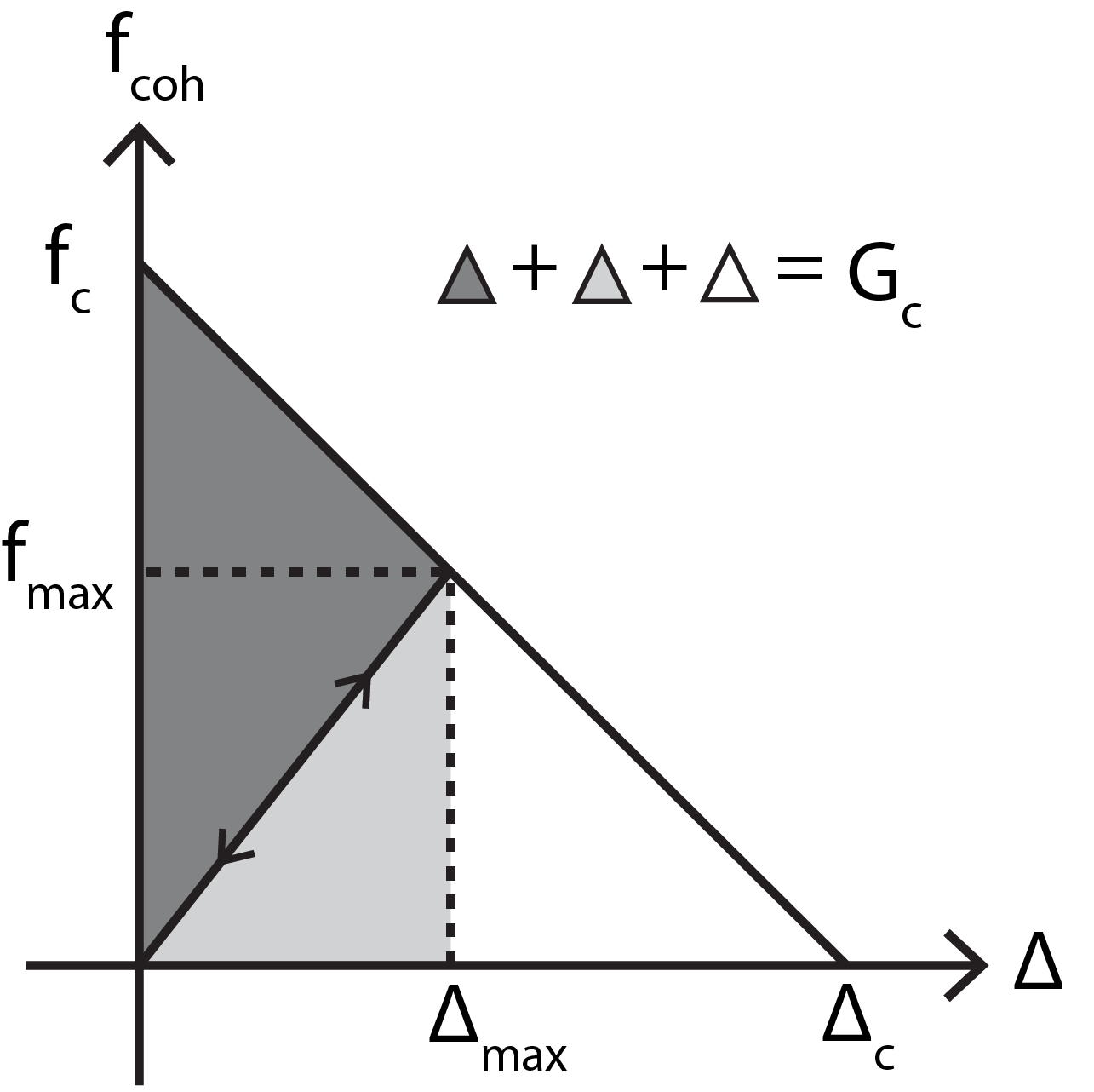
Figure 4: The force-separation cohesive law prescribes a linear decay of the scalar effective cohesive force $f_{coh}$ with the scalar effective separation $\Delta$, from a critical value $f_{c}$ to zero. Irreversibility is modeled by introducing a history variable $\Delta_{max}$ representing the maximum effective separation achieved. The unloading path follows a trajectory back to the origin, while reloading occurs on the same unloading path. Complete fracture is achieved when $\Delta\geq\Delta_{c}$.

Specifically, in the loading stage, we set:

$$f_{coh}(\Delta,\Delta_{max})=\Bigg{(}1-\frac{\Delta}{\Delta_{c}}\Bigg{)}\>f_{c}\quad\text{for}\quad\Delta\geq\Delta_{max},$$ (24)

where $\Delta_{max}$ is the maximum effective separation in the entire loading history, $\Delta_{c}=2G_{c}/\sigma_{c}$ is the effective separation at which complete decohesion occurs, and $G_{c}$ is the effective fracture energy. In the unloading and reloading stage, we set:

$$f_{coh}(\Delta,\Delta_{max})=\frac{\Delta}{\Delta_{max}}f_{max}\quad\text{for}\quad\Delta<\Delta_{max},$$ (25)

where $f_{max}$ is the effective cohesive force at $\Delta_{max}$.

The cohesive laws described above are activated at an inter-element boundary of the beam upon meeting the following fracture initiation criterion:

$$f_{eq}(\langle\boldsymbol{f}\rangle,\langle\boldsymbol{m_{\perp}}\rangle)\geq f_{c},$$ (26)

where $f_{c}=\sigma_{c}A$ is the critical effective cohesive force expressed in terms of the material’s cohesive strength $\sigma_{c}$, and $f_{eq}$ is an equivalent force given by the scalar:

$$f_{eq}(\boldsymbol{f},\boldsymbol{m_{\perp}})=\sqrt[]{\{\boldsymbol{f}\cdot\boldsymbol{\hat{n}_{coh}}\}^{2}+\Bigg{|}\Bigg{|}\frac{\boldsymbol{m_{\perp}}}{\alpha R}\Bigg{|}\Bigg{|}^{2}}.$$ (27)

3.3 The discontinuous Galerkin / cohesive zone model weak formulation

As discussed in Section 3, within the discontinuous Galerkin / cohesive zone model framework, the position and tangent fields are allowed to exhibit discontinuities at the boundaries of the finite elements. However, prior to fracture, the solution’s compatibility across element boundaries is maintained via the variationally-consistent interface forces and moments derived in that section.

Upon satisfaction of the fracture criterion (26), the interface axial forces and bending moments in Equation (19) are replaced with the cohesive axial forces and the cohesive bending moments of Equation (23). However, because we assume negligible shear strains and, consistently, we do not model the shear modes of fracture, we ensure that the component of the interface force term perpendicular to the unit normal of the cohesive boundary in Equation (19) remains active until complete interface failure [20]. Specifically, this is achieved by introducing two binary parameters $\alpha_{n}$ and $\gamma_{n}$, which take value at each interface $n$. While we set both $\alpha_{n}=1$ and $\gamma_{n}=1$ before fracture initiation, we set $\alpha_{n}=0$ after the fracture criterion (26) is met, and $\gamma_{n}=0$ upon complete decohesion (i.e. $\Delta\geq\Delta_{c}$).

The discontinuous Galerkin / cohesive zone model weak form reads, therefore:

$$\int_{\Omega_{h}}\rho A\boldsymbol{\ddot{r}}\cdot\boldsymbol{\delta r}\>ds +\int_{\Omega_{h}}EA\>\varepsilon\>\delta\varepsilon\>ds+\sum_{n=1}^{E-1}\>\alpha_{n}\Big{[}\boldsymbol{f_{DG,\>||}}\cdot[\![\boldsymbol{\delta r}]\!]\Big{]}\Big{|}_{s_{n}}+\sum_{n=1}^{E-1}\>\gamma_{n}\Big{[}\boldsymbol{f_{DG,\>\perp}}\cdot[\![\boldsymbol{\delta r}]\!]\Big{]}\Big{|}_{s_{n}}$$ (28)

$$+\sum_{n=1}^{E-1}\>\alpha_{n}\Bigg{[}\beta_{p}\bigg{\langle}\frac{EA}{h}\bigg{\rangle}\>\boldsymbol{c_{DG,\>||}}\cdot[\![\boldsymbol{\delta r}]\!]\Bigg{]}\Bigg{|}_{s_{n}}+\sum_{n=1}^{E-1}\>\gamma_{n}\Bigg{[}\beta_{p}\bigg{\langle}\frac{EA}{h}\bigg{\rangle}\>\boldsymbol{c_{DG,\>\perp}}\cdot[\![\boldsymbol{\delta r}]\!]\Bigg{]}\Bigg{|}_{s_{n}}$$

$$+\int_{\Omega_{h}}EI\>\boldsymbol{\kappa}\cdot\boldsymbol{\delta\kappa}\>ds+\sum_{n=1}^{E-1}\>\alpha_{n}\Big{[}\langle\boldsymbol{m_{\perp}}\rangle\cdot[\![\boldsymbol{\delta\theta}]\!]\Big{]}\Big{|}_{s_{n}}+\sum_{n=1}^{E-1}\>\alpha_{n}\Bigg{[}\beta_{t}\bigg{\langle}\frac{EI}{h}\bigg{\rangle}[\![\boldsymbol{g_{1}}]\!]\cdot[\![\boldsymbol{\delta g_{1}}]\!]\Bigg{]}\Bigg{|}_{s_{n}}$$

$$+\sum_{n=1}^{E-1}\>(1-\alpha_{n})\Big{[}\boldsymbol{f_{coh,\>||}}\cdot[\![\boldsymbol{\delta r}]\!]\Big{]}\Big{|}_{s_{n}}+\sum_{n=1}^{E-1}\>(1-\alpha_{n})\Big{[}\boldsymbol{m_{coh,\>\perp}}\cdot[\![\boldsymbol{\delta g_{1}}]\!]\Big{]}\Big{|}_{s_{n}}$$

$$=\int_{\Omega_{h}}\boldsymbol{\tilde{f}} \cdot\boldsymbol{\delta r}\>ds+\left(\boldsymbol{\bar{f}}\cdot\boldsymbol{\delta r}\right)\Big{|}_{\partial_{N_{f}}\Omega_{h}}+\int_{\Omega_{h}}\boldsymbol{\tilde{m}_{\perp}}\cdot\boldsymbol{\delta\theta}\>ds+\left(\boldsymbol{\bar{m}_{\perp}}\cdot\boldsymbol{\delta\theta}\right)\Big{|}_{\partial_{N_{m}}\Omega_{h}}$$

where we have set:

$$\boldsymbol{f_{DG,\>||}} =\left(\langle\boldsymbol{f}\rangle\cdot\boldsymbol{\hat{n}_{coh}}\,\right)\,\boldsymbol{\hat{n}_{coh}},$$

$$\boldsymbol{f_{DG,\>\perp}} =\left(\boldsymbol{I}-\boldsymbol{\hat{n}_{coh}}\otimes\boldsymbol{\hat{n}_{coh}}\right)\langle\boldsymbol{f}\rangle,$$

$$\boldsymbol{c_{DG,\>||}} =\left([\![\boldsymbol{r}]\!]\cdot\boldsymbol{\hat{n}_{coh}}\,\right)\,\boldsymbol{\hat{n}_{coh}},$$

$$\boldsymbol{c_{DG,\>\perp}} =\left(\boldsymbol{I}-\boldsymbol{\hat{n}_{coh}}\otimes\boldsymbol{\hat{n}_{coh}}\right)[\![\boldsymbol{r}]\!].$$

Finally, in case of contact occurring after fracture initiation (i.e. when $\Delta_{||}<0$ and $\Delta_{max}>0$), we reactivate the variationally-consistent axial forces and the position stabilization term, so as to allow propagation of compressive stress waves across cracked interfaces.

3.4 Discretization in space and time

Because of the high-order derivatives involved in the weak formulation, we discretize $\boldsymbol{r}$ in space with third-order Hermite polynomials as follows:

$$\boldsymbol{r}(\xi)\approx\sum_{b=1}^{2}N_{p}^{b}(\xi)\boldsymbol{p}^{b}+\frac{L}{2}\sum_{b=1}^{2}N_{t}^{b}(\xi)\boldsymbol{t}^{b}:=\sum_{a=1}^{4}N_{a}(\xi)\boldsymbol{x_{a}}$$ (29)

where $\boldsymbol{p}^{b}$ and $\boldsymbol{t}^{b}$ are the position and tangent degrees of freedom at the element nodes $b=1,2$, $\xi\in[-1,1]$ is the parametric coordinate in the reference element, which is mapped to the arc-length coordinate $s\in[0,L]$ as $s=\frac{L}{2}(1+\xi)$, and $N_{p}^{b}$ and $N_{t}^{b}$ are the following shape functions:

$$N_{p}^{1}(\xi) =\frac{1}{4}(2+\xi)(1-\xi)^{2}\>;\>\>N_{p}^{2}(\xi)=\frac{1}{4}(2-\xi)(1+\xi)^{2},$$

$$N_{t}^{1}(\xi) =\frac{1}{4}(1+\xi)(1-\xi)^{2}\>;\>\>N_{t}^{2}(\xi)=-\frac{1}{4}(1-\xi)(1+\xi)^{2}.$$

This space discretization results in the following semi-discrete system of equations:

$$\boldsymbol{M_{ab}}\boldsymbol{\ddot{x}_{b}}+\boldsymbol{f^{int}_{a}}+\boldsymbol{f^{jump}_{a^{\pm}}}=\boldsymbol{f^{ext}_{a}},$$ (30)

where the inertia $\boldsymbol{M_{ab}}\boldsymbol{\ddot{x}_{b}}$, internal (bulk) $\boldsymbol{f^{int}_{a}}$, internal (interface) $\boldsymbol{f^{jump}_{a^{\pm}}}$, and external $\boldsymbol{f^{ext}_{a}}$ forces are reported in A.

We discretize Equation (30) in time using the second-order explicit Newmark scheme. We perform a special mass lumping [42] to avoid the cost of solving a linear system for computing the accelerations. As explicit time stepping schemes are conditionally stable, we compute the stable time step $\Delta t_{c}$ from the Courant-Friedrichs-Lewy condition:

$$\Delta t_{c}=\frac{2}{\omega_{max}},$$ (31)

where $\omega_{max}=\max_{i=1}^{N}(||\lambda_{i}||)$ is the maximum natural frequency of the system.

In our simulations, we compute the stable time step $\Delta t_{c}$ only once at the beginning of the calculation and we set $\Delta t=\Delta t_{c}$ for the entire calculation. Specifically, we calculate $\Delta t_{c}$ by solving the following linearized eigenvalue problem:

$$\left(\boldsymbol{K_{ab}^{int}}+\boldsymbol{K_{ab^{\pm}}^{jump,DG}}-\lambda^{2}\>\boldsymbol{M_{ab}^{lump}}\right)\boldsymbol{\Phi}=\boldsymbol{0},$$ (32)

where $\lambda$ and $\boldsymbol{\Phi}$ are the eigenvalue and eigenvector pair, $\boldsymbol{M_{ab}^{lump}}$ is the lumped mass matrix, and matrices $\boldsymbol{K_{ab}^{int}}$ and $\boldsymbol{K_{ab^{\pm}}^{jump,DG}}$ are reported in B. It should be noted that the eigenvalues obtained by solving Equation (32) may be complex since matrix $\boldsymbol{K_{ab^{\pm}}^{jump,DG}}$ is not symmetric.

4 Results

This section presents verification and validation of our computational framework.

4.1 Framework verification: Buckling of a slender column

We first verify our computational framework in the absence of fracture for the case of a column buckling under quasi-static axial compression. Specifically, we consider a slender column of length $L$, radius $R$ and Young’s modulus $E$ and we verify that the first buckling mode occurs at Euler’s critical axial force:

$$f_{cr}=\frac{\pi^{3}}{4}\frac{ER^{4}}{L^{2}}.$$ (33)

The problem geometry and boundary conditions considered are illustrated in Figure 5. We apply a pin support at the bottom end of the column ($x=y=0$), and a roller support allowing displacement in the $x$-direction at the top end ($x=L\>,\>y=0$), where we also impose a displacement in the negative $x$ direction, ramping up quasi-statically to a maximum $\Delta$ through 1000 load steps. In addition, we apply a constant perturbation force $P$ at the center of the column ($x=L/2\>,\>y=0$) as a means to break the symmetry of the problem. Table 1 summarizes the physical properties and numerical parameters used.

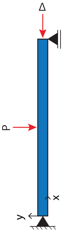
Figure 5: Schematic of the geometry and boundary conditions for the slender column buckling benchmark. The column is supported with a pin at the bottom end, a roller at the top end, and is loaded with an imposed axial displacement $\Delta$. To facilitate the occurrence of the buckling bifurcation, a small, transverse perturbation force $P$ is applied at the center of the column to break the problem’s symmetry.

Property / Parameter	Value
Length ($L$)	$10\>m$
Radius ($R$)	$0.1\>m$
Young’s modulus ($E$)	$200.0\>GPa$
Final applied displacement ($\Delta$)	$5.0\>mm$
Applied perturbation force ($P$)	$1.0\>N$
Mesh size ($h$)	$1.0\>m$
Penalty parameters ($\beta_{p,n}$ and $\beta_{t,n}$)	10

Table 1: Physical properties and numerical parameters used in the slender column buckling benchmark.

We apply our DG/CZM computational framework to solve the problem in a quasi-static setting using a Newton-Raphson solver with the linearization provided in B. Figure 6 shows that the load-displacement response of the column is in agreement with the theoretical predictions.

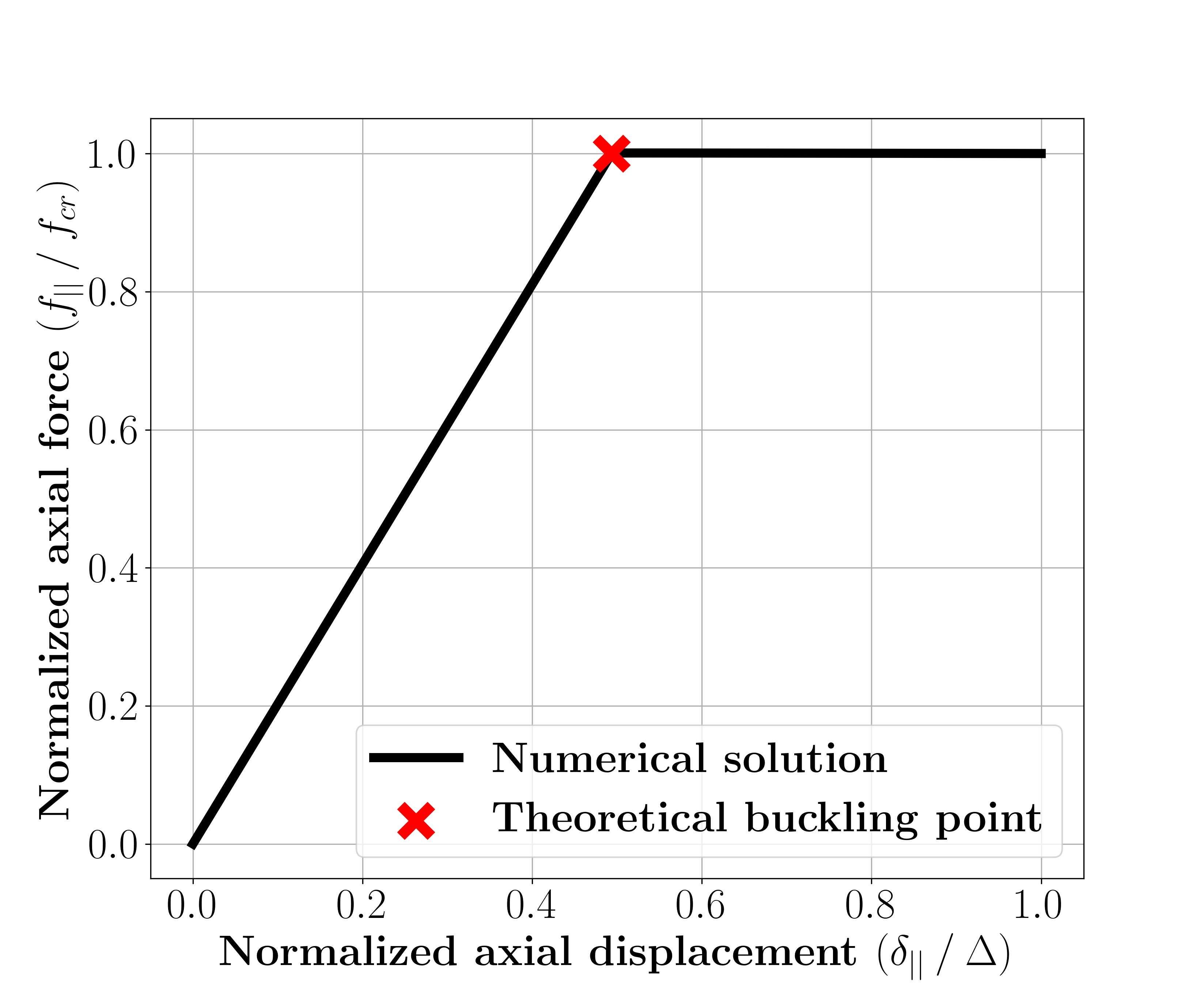
Figure 6: Verification of our computational framework in the case of buckling of a slender column. The plot shows the force-displacement response at the top end of the column. The axial force $f_{||}$ is normalized with respect to the theoretical critical axial force $f_{cr}$, while the axial displacement $\delta_{||}$ is normalized with respect to the final applied displacement $\Delta$. The theoretical buckling point is marked with a cross.

4.2 Framework verification: Fracture of a slender bar under tension

We verify the fracture modeling capability of our computational framework by simulating the spall of a bar, i.e. the development of a crack as a result of the interaction of two tensile stress waves. We consider a slender bar subjected to tensile axial loading, while transverse displacement is restrained through roller supports at the bar ends, as illustrated in Figure 7. We apply the following axial displacement signal:

$$\delta(t)=\frac{\sigma_{f}}{2}\frac{t}{\rho c_{l}},$$ (34)

where $c_{l}=\sqrt{E/\rho}$ is the bar longitudinal wave speed and $\sigma_{f}$ is a stress loading factor. Table 2 summarizes the physical properties and the numerical parameters used in this computational experiment.

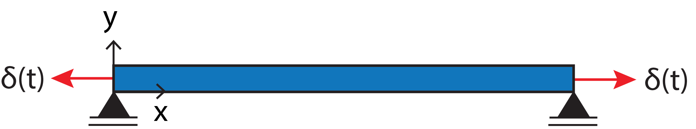
Figure 7: Schematic of the geometry and boundary conditions for the bar spall benchmark. The axial displacement signal $\delta(t)$ in Equation (34) is applied at the two ends of the bar, while two roller supports restrain the transverse displacement.

Property / Parameter	Value
Length ($L$)	$0.1\>m$
Radius ($R$)	$1.0\>mm$
Mass density ($\rho$)	$3690\>kg\ m^{-3}$
Young’s modulus (E)	$260.0\>GPa$
Critical cohesive strength ($\sigma_{c}$)	$400.0\>MPa$
Fracture energy ($G_{c}$)	$100.0\>N\ m^{-1}$
Mode-mixity parameter ($\alpha$)	$1$
Simulation time ($T$)	$10\>\mu s$
Mesh size ($h$)	$0.1\>mm$
Time step ($\Delta t$)	$0.01\>ns$
Penalty parameters ($\beta_{p,n}$ and $\beta_{t,n}$)	$10$

Table 2: Physical properties and numerical parameters used in the bar spall benchmark.

We apply our DG/CZM computational framework to model the dynamic response of the bar with two values of $\sigma_{f}$, namely $\sigma_{f}=0.1\ \sigma_{c}$ and $\sigma_{f}=\sigma_{c}$. Figure 8 presents the evolution of the axial stress response over time obtained in our simulations, against the corresponding analytical solution to the 1D wave equation. It can be observed that the applied displacement signal generates two tensile stress waves with step waveform and intensity $\sigma_{f}/2$ propagating inwards from the beam ends. The two tensile waves meet at the center of the bar, building up a tensile stress wave of intensity $\sigma_{f}$. When $\sigma_{f}$ is less than the critical fracture strength $\sigma_{c}$, our results show that the bar remains undamaged, as expected. When $\sigma_{f}$ is equal to the critical fracture strength $\sigma_{c}$, our results capture the fracture response, including the development of a release wave and the subsequent vanishing of the axial stress due to the creation of a free surface. Figure 9 presents snapshots of the simulated bar response showing the bar deformation the propagation of the stress waves in the bar before and after fracture.

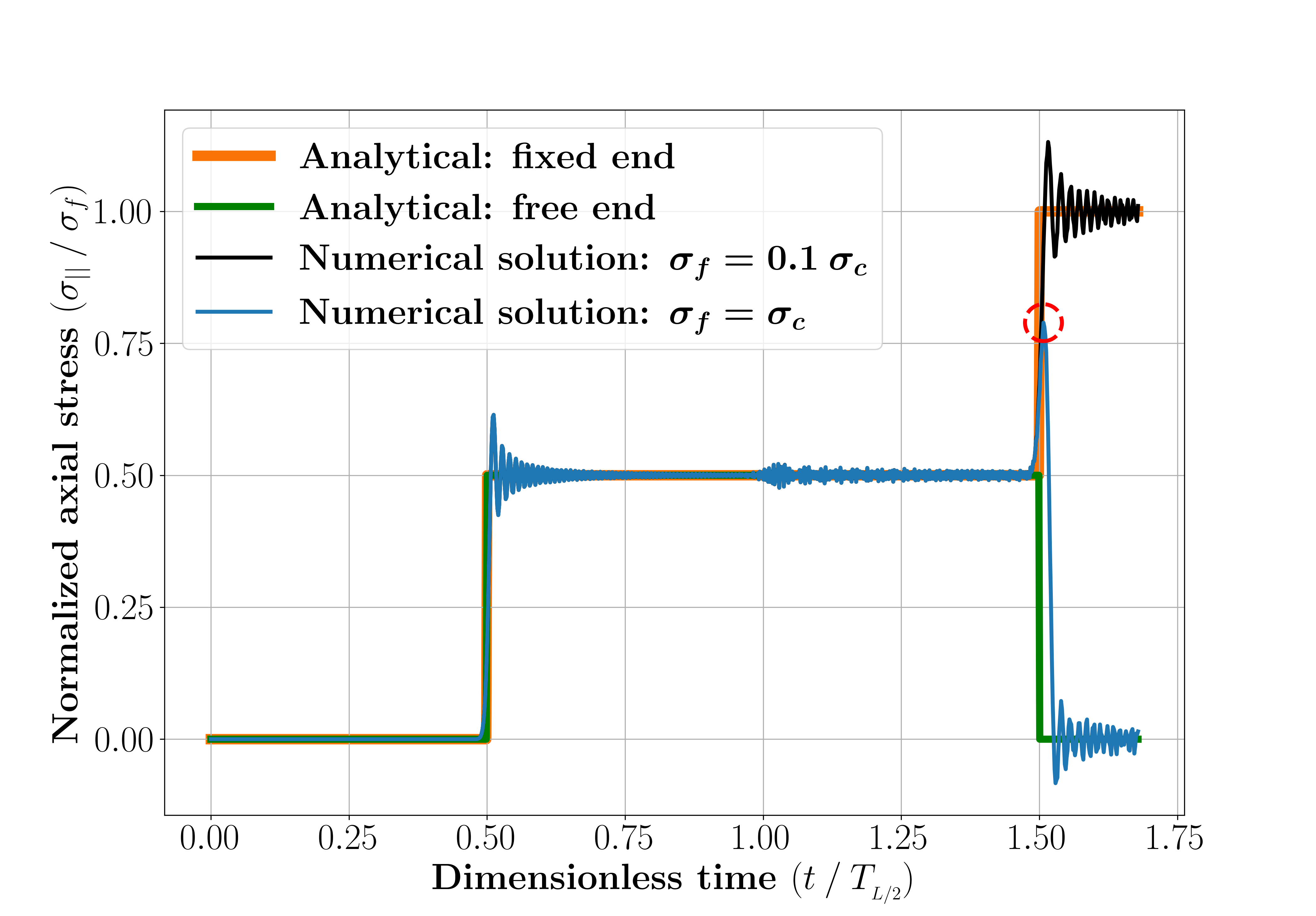
Figure 8: Verification of our computational framework applied to the fracture of a slender bar under tensile load. The plot shows a comparison of the simulated and theoretical axial stress evolution in time, gauged at a point $L/4$ from the bar end, for two different applied displacement signals (Equation (34)), one with $\sigma_{f}<\sigma_{c}$ (no fracture) and the other with $\sigma_{f}=\sigma_{c}$ (fracture). The theoretical predictions correspond to the solution of the 1D wave equation on a bar of half length with the same applied displacement signal on one end and the other end fixed (no fracture) or free (fracture). The axial stress $\sigma_{||}=E\varepsilon$ is normalized with respect to the applied stress $\sigma_{f}$, while the time is normalized with respect to $T_{L/2}=L/(2c_{l})$, which is the time when the longitudinal stress waves meet at the center of the bar. We observe that, when $\sigma_{f}<\sigma_{c}$, our numerical results match closely with the theoretical response of an uncracked bar. Conversely, when $\sigma_{f}=\sigma_{c}$, our results correctly capture the fracture event at $t=T_{L/2}$ resulting from the interaction of the two tensile waves. Note that the axial force signal at the gauge location ($x=L/4$) follows the uncracked solution until time $t=1.5\ T_{L/2}$, that is the time when the gauge is reached by the release wave arising from the fracture event (see red circle). Subsequently, our results correctly portray the vanishing of the axial force due to the fully developed fracture at the center of the beam.

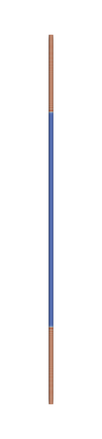
(a)

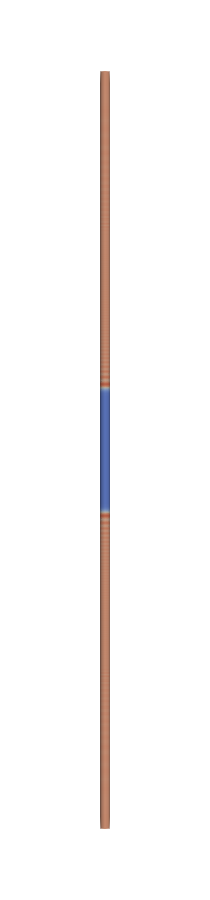
(b)

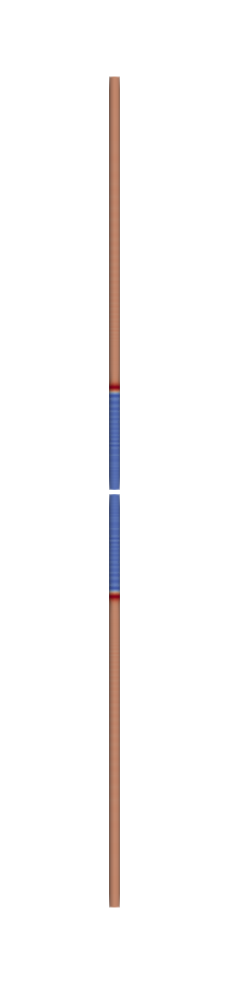
(c)

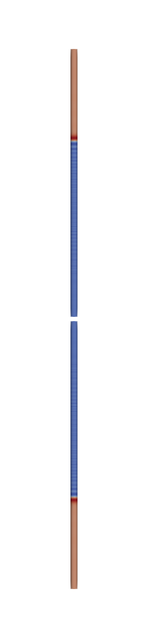
(d)

Figure 9: Snapshots of pre-fracture and post-fracture evolution of the bar deformation and axial force at times: (a) $0.42\ T_{L/2}$, (b) $0.84\ T_{L/2}$, (c) $1.26\ T_{L/2}$, and (d) $1.68\ T_{L/2}$. The bar is shown in its deformed configuration (displacements are scaled by a factor of 10 for better visualization) and the contours show the axial forces in the bar. We observe the propagation of the two tensile step waves towards the center of the bar (pictures (a) and (b)), the creation of a fracture surface as a result of their interaction at the center, as well as the reflection of the stress waves at the newly created free surface (pictures (c) and (d)).

4.3 Fracture of a bar under transverse load

Through this example, we demonstrate the significance of incorporating inter-element jumps in the tangent degrees of freedom and of modeling the relaxation of the bending moments as a function of these jumps, in the spirit of the well-established traction-separation laws of fracture mechanics. This is in contrast to the computational framework for fracture in geometrically exact beams proposed by Tojaga et al. [31], where only the displacement degrees of freedom are enriched with discontinuous modes, but not the rotation ones.

We consider a slender bar cantilevered at both ends and loaded at the center, as illustrated in Figure 10. Specifically, we apply a time-dependent transverse displacement $\delta(t)$:

$$\delta(t)=\tilde{v}t$$ (35)

where $\tilde{v}$ is a sufficiently low loading rate to achieve quasi-static conditions. Table 3 summarizes the physical properties and the numerical parameters used in this computational experiment.

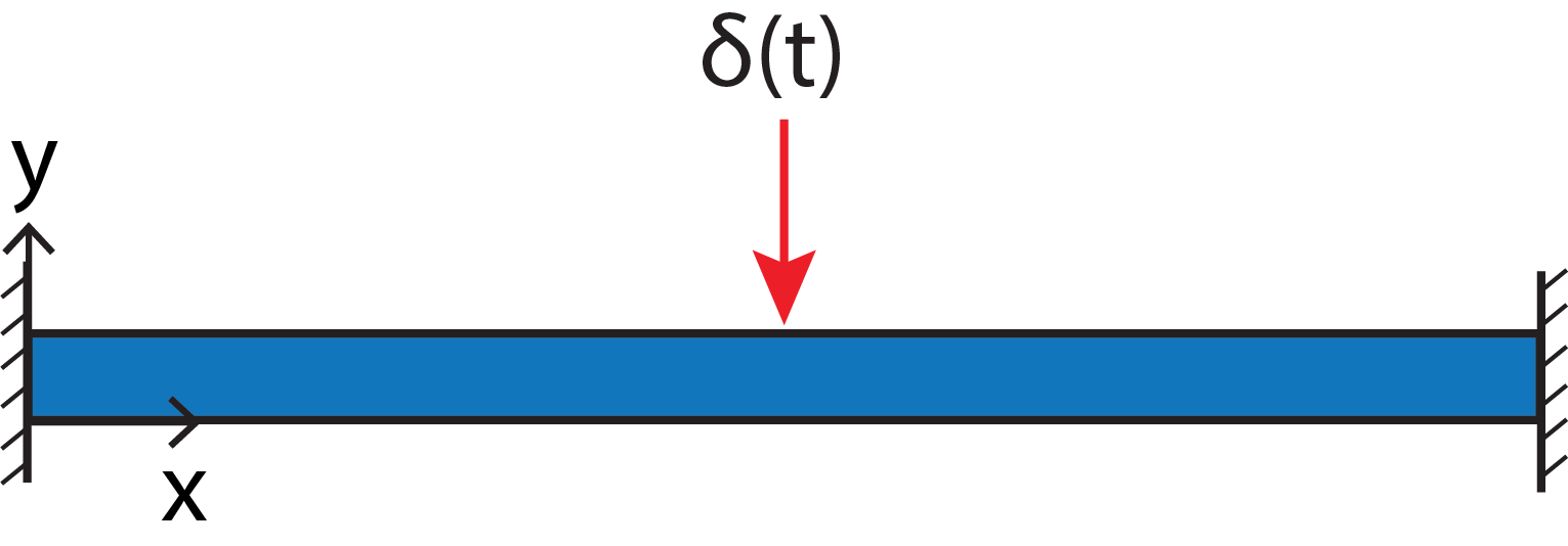
Figure 10: Schematic of the geometry and boundary conditions for the problem of a bar under transverse load. The beam is cantilevered at both ends and loaded at the center with a time-dependent transverse displacement $\delta(t)$, see Equation (35).

Property / Parameter	Value
Length ($L$)	$0.1\>m$
Radius ($R$)	$1.0\>mm$
Mass density ($\rho$)	$3690\>kg\ m^{-3}$
Young’s modulus (E)	$260.0\>GPa$
Critical cohesive strength ($\sigma_{c}$)	$400.0\>MPa$
Fracture energy ($G_{c}$)	$100.0\>N\ m^{-1}$
Mode-mixity parameter ($\alpha$)	$1$
Load rate ($\tilde{v}$)	$0.01\>m\>s^{-1}$
Simulation time ($T$)	$0.2\>s$
Mesh size ($h$)	$0.1\>mm$
Time step ($\Delta t$)	$0.1\>\mu s$
Penalty parameters ($\beta_{p,n}$ and $\beta_{t,n}$)	$10$

Table 3: Physical properties and numerical parameters used in the bar under transverse load problem.

We solve this problem computationally with two different approaches: 1) our DG/CZM computational framework as described in Section 3, and 2) a variant of such framework that does not model the bending moment decay with the increasing tangents jumps (i.e. removing the bending moment term in Equation (27)). Figure 11 compares the load-displacement responses of the center of the bar obtained with these two approaches. The figure shows the bending moments build-up with the increasing applied displacement, including the transition from the geometrically linear to the geometrically nonlinear regime. We observe that our DG/CZM approach is able to capture the fracture behavior arising from a further increase in applied displacement, along with the vanishing bending moment in the post-fracture behavior. This stands in stark contrast to the second approach, which predicts a load-displacement response identical to that of a simulation without an embedded fracture mechanics model (pure DG). This demonstrates the essential role of explicitly modeling jumps in the tangent degrees of freedom to capture the bending fracture mode.

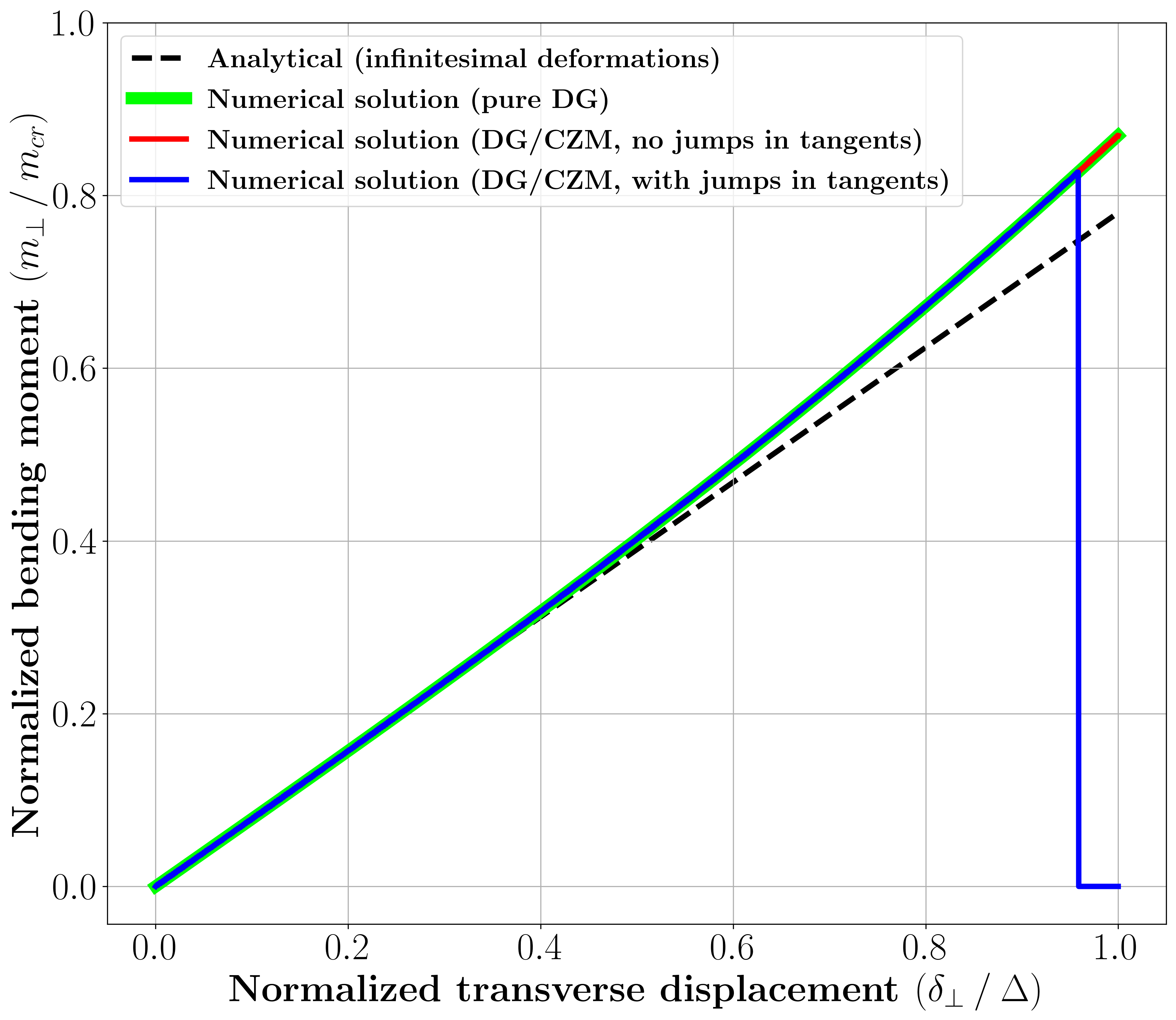
Figure 11: The load-displacement response at the center of a bar fracturing under transverse load, in terms of bending moment versus applied transverse displacement. Simulation results are plotted on top of the analytical predictions of Euler-Bernoulli beam theory (dashed line) to highlight the departure from the geometrically linear regime. The bending moment is normalized with respect to the critical bending moment $m_{cr}=AR\sigma_{c}$, where $A$ is the area of the beam cross section, while the transverse displacement of the beam is normalized with respect to the maximum applied transverse displacement $\Delta=\tilde{v}T$. The plot compares simulation results obtained with our DG/CZM computational framework when incorporating discontinuities in the tangent degrees of freedom across adjacent elements (blue line) and when not incorporating them (red line). In the first case, the simulation is able to capture the bar failure under bending in the geometrically nonlinear range, and the resulting drop in the bending moment. In the second case, the simulation does not capture the fracture behavior and the bending moment follows the response predicted by a simulation without an embedded fracture mechanics model (green line).

We also observe that, under these conditions, fracture occurs in mixed bending and tensile modes, as complete fracture is achieved for an internal moment $m_{\perp}\approx 0.8\ m_{cr}<m_{cr}$, where $m_{cr}=AR\sigma_{c}$, where $A$ is the area of the beam cross section, see Figure 11.

Figure 12 presents snapshots of the simulated bar response showing the bar configuration before and after fracture.

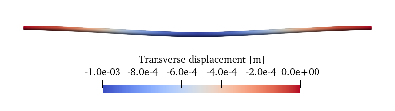
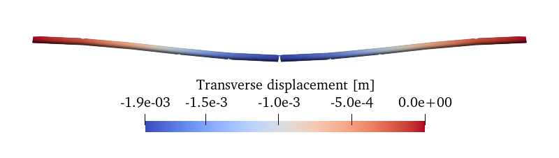
Figure 12: Snapshots of the simulated bar response before (top picture, $\delta(t)=1.0\ mm$) and after (bottom picture, $\delta(t)=1.92\ mm$) fracture. The bar is shown in its deformed configuration (displacements are scaled by a factor of 2 for better visualization) and the contours show the transverse displacement.

4.4 Framework validation: Fracture of a bar bent and suddenly released

In this section, we validate our computational framework against experiments by Audoly and Neukirch [18] on the fragmentation of dry spaghetti. Specifically, that work presents experiments on dry spaghetti rods initially bent into an arc of circle and suddenly released at one end, while the other end remains clamped. The experiments show that this sudden relaxation of curvature results in a burst of flexural waves, which locally increase the curvature of the rod, ultimately leading to fracture.

We model these experiments with a two-stage solution strategy. As in experiments [18], the spaghetti rod remains clamped at one end in both stages of the analysis. In the first stage, we perform a quasi-static simulation using a Newton-Raphson solver with the linearization provided in B to bring the spaghetti rod to a curvature $\kappa_{0}$. Specifically, we apply a nodal moment of $EI\kappa_{0}$ at the free end of the rod in $10$ load steps. Note that this initial pre-loading stage is necessary because of our model’s assumption that the beam be straight in the reference (unstressed) configuration. The state achieved through the quasi-static pre-loading stage is then used as the initial condition for a dynamic simulation starting with the release of the spaghetti rod’s free end. The physical properties and numerical parameters used in this computational experiment are summarized in Table 4. Specifically, we used the length $L$, radius $R$, and density $\rho$ values reported in Heisser et al.  [30] and we computed the Young’s modulus $E$ of the spaghetti rods with the formula $E=\gamma^{2}\rho A/I$, where $\gamma=0.521\>m^{2}/s$, see [18]. Finally, we obtained $\sigma_{c}$, and $G_{c}$ based on the time and deformation shape of the rod reported in the experiments just before fracture.

Figure 13 shows contours of bending moments on the deformed spaghetti rods, superimposed to the experimentally observed deformed shapes at different times. Our DG/CZM framework accurately captures the fracture mechanism observed in the experiments, including the burst of flexural waves and the curvature build-up in the proximity of the clamped end.

Property / Parameter	Value
Length ($L$)	$0.24\>m$
Radius ($R$)	$0.57\>mm$
Mass density ($\rho$)	$1400\>kg\ m^{-3}$
Young’s modulus (E)	$5.5\>GPa$
Critical cohesive strength ($\sigma_{c}$)	$25\>MPa$
Fracture energy ($G_{c}$)	$1500\>N\ m^{-1}$
Mode-mixity parameter ($\alpha$)	$1$
Initial curvature ($\kappa_{0}$)	$14.18\>rad\>s^{-1}$
Simulation time ($T$)	$0.01\>s$
Mesh size ($h$)	$2.4\>mm$
Time step ($\Delta t$)	$0.1\>\mu s$
Penalty parameters ($\beta_{p,n}$ and $\beta_{t,n}$)	$10$

Table 4: Physical properties and numerical parameters used in the bent and released spaghetti problem.

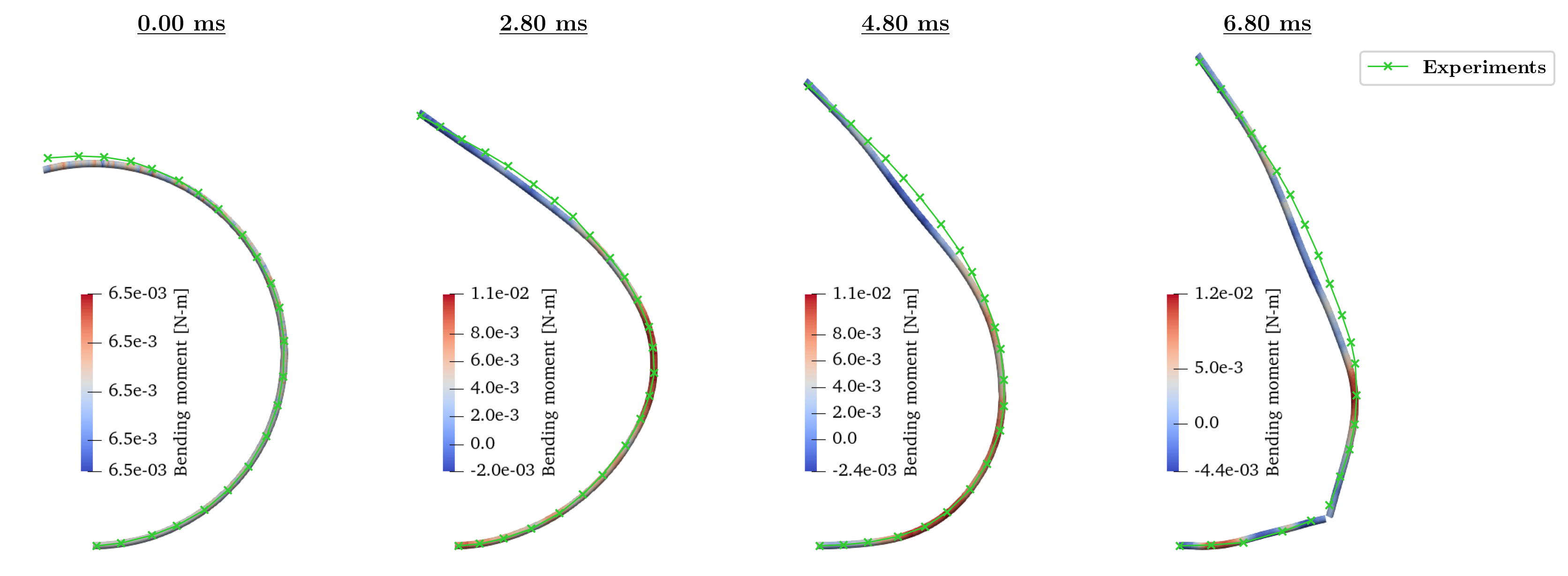
Figure 13: Validation of our computational framework against fracture experiments of bent and released spaghetti rods [18]. The pictures show the deformed spaghetti shapes obtained in our computational predictions overlaid to those observed experimentally (green line). Our DG/CZM framework captures the local curvature build-up due to the flexural waves generated by the release, the resulting increase of bending moment (shown in the contours), as well as the ultimate fracture event. An animation of the time evolution of this simulation is provided in the Supplementary Material.

5 Conclusions

We presented a computational framework to simulate fracture in slender beams subjected to large deformations in three-dimensional space. We adopted the geometrically exact Kirchhoff beam formulation proposed by Meier et al. [36] to model the complex geometric nonlinearities involved in the beam deformation. We developed a discontinuous Galerkin discretization of the beam governing equations incorporating jumps in position and tangent degrees of freedom. In our framework, compatibility of nodal positions and tangents is weakly enforced before fracture initiation via the exchange of variationally-consistent forces and moments at the interfaces between adjacent elements. At the onset of fracture, these forces and moments transition to cohesive laws modeling softening of the stress-resultant forces and moments with the increasing interface separation. We showed that incorporating discontinuities in the tangent degrees of freedom across adjacent elements is essential for capturing beam fracture under bending. We conducted a series of numerical tests to verify our framework’s ability to capture tensile and bending fracture modes in slender beams. Finally, we applied our computational framework to reproduce experiments by Audoly and Neukirch [18] on the dynamic fracture behavior of dry spaghetti rods exhibiting large deformations.

Declaration of generative AI and AI-assisted technologies in the writing process

During the preparation of this work the author(s) used ChatGPT in order to expedite the language editing process (e.g. to rewrite particularly complex sentences in a clearer way). After using this tool/service, the author(s) reviewed and edited the content as needed and take(s) full responsibility for the content of the publication.

Appendix A Inertia, internal, and external forces in the semi-discrete system of equations

This Appendix reports the expressions of the inertia, internal (bulk), internal (interface), and external forces discussed in Section 3.4.

$$\boldsymbol{M_{ab}}\boldsymbol{\ddot{x}_{b}}=\Bigg{[}\int_{-1}^{1}N_{a}\rho AN_{b}\frac{L}{2}\>d\xi\Bigg{]}\boldsymbol{\ddot{x}_{b}},$$

$$\boldsymbol{f^{int}_{a}}=\int_{-1}^{1}\big{[}N_{a}^{\prime}(EA\boldsymbol{t_{1}}+EI\boldsymbol{t_{2}})+N_{a}^{\prime\prime}EI\boldsymbol{t_{3}}\big{]}\frac{L}{2}\>d\xi,$$

$$\boldsymbol{f^{jump}_{a^{\pm}}}=\pm\sum_{n=1}^{E-1}\>\alpha_{n}\Bigg{[}\Big{[}N_{a}\boldsymbol{f_{DG,\>||}}\Big{]}+\Big{[}N_{a}^{\prime}\big{[}\langle\boldsymbol{m_{\perp}}\rangle\times\boldsymbol{t_{4}}\big{]}\Big{]}+\beta_{p}\bigg{\langle}\frac{EA}{h}\bigg{\rangle}\Big{[}N_{a}\boldsymbol{c_{DG,\>||}}\Big{]}$$

$$+\>\beta_{t}\bigg{\langle}\frac{EI}{h}\bigg{\rangle}\Big{[}N_{a}^{\prime}\,\boldsymbol{t_{5}}\Big{]}\Bigg{]}\Bigg{|}_{s_{n}}\pm\sum_{n=1}^{E-1}\>\gamma_{n}\Bigg{[}\Big{[}N_{a}\boldsymbol{f_{DG,\>\perp}}\Big{]}+\beta_{p}\bigg{\langle}\frac{EA}{h}\bigg{\rangle}\Big{[}N_{a}\boldsymbol{c_{DG,\>\perp}}\Big{]}\Bigg{]}\Bigg{|}_{s_{n}}$$

$$\pm\sum_{n=1}^{E-1}\>(1-\alpha_{n})\Bigg{[}\Big{[}N_{a}\boldsymbol{f_{coh,\>||}}\Big{]}+\Big{[}N_{a}^{\prime}\boldsymbol{G_{1}}\boldsymbol{m_{coh,\>\perp}}\Big{]}\Bigg{]}\Bigg{|}_{s_{n}},$$

$$\boldsymbol{f^{ext}_{a}}=\int_{-1}^{1}\big{[}N_{a}\boldsymbol{\tilde{f}}+N_{a}^{\prime}(\boldsymbol{\tilde{m}_{\perp}}\times\boldsymbol{t_{4}})\big{]}\frac{L}{2}\>d\xi+\big{[}N_{a}\boldsymbol{\bar{f}}\,\big{]}\big{|}_{\partial_{N_{f}}\Omega_{h}}+\big{[}N_{a}^{\prime}(\boldsymbol{\bar{m}_{\perp}}\times\boldsymbol{t_{4}})\big{]}\big{|}_{\partial_{N_{m}}\Omega_{h}},$$

where

$$\boldsymbol{t_{1}}=\frac{\boldsymbol{r^{\prime}}}{||\boldsymbol{r^{\prime}}||}\big{(}||\boldsymbol{r^{\prime}}||-1\big{)},$$

$$\boldsymbol{t_{2}}=\frac{2\boldsymbol{r^{\prime}}\big{(}\boldsymbol{r^{\prime}}\cdot\boldsymbol{r^{\prime\prime}}\big{)}^{2}}{||\boldsymbol{r^{\prime}}||^{6}}-\Bigg{[}\frac{\boldsymbol{r^{\prime}}\big{(}\boldsymbol{r^{\prime\prime}}\cdot\boldsymbol{r^{\prime\prime}}\big{)}+\boldsymbol{r^{\prime\prime}}\big{(}\boldsymbol{r^{\prime}}\cdot\boldsymbol{r^{\prime\prime}}\big{)}}{||\boldsymbol{r^{\prime}}||^{4}}\Bigg{]},$$

$$\boldsymbol{t_{3}}=\frac{\boldsymbol{r^{\prime\prime}}}{||\boldsymbol{r^{\prime}}||^{2}}-\frac{\boldsymbol{r^{\prime}}\big{(}\boldsymbol{r^{\prime}}\cdot\boldsymbol{r^{\prime\prime}}\big{)}}{||\boldsymbol{r^{\prime}}||^{4}},$$

$$\boldsymbol{t_{4}}=\frac{\boldsymbol{r^{\prime}}}{||\boldsymbol{r^{\prime}}||^{2}},$$

$$\boldsymbol{G_{1}}=\frac{\boldsymbol{I}}{||\boldsymbol{r^{\prime}}||}-\frac{(\boldsymbol{r^{\prime}}\otimes\boldsymbol{r^{\prime}})}{||\boldsymbol{r^{\prime}}||^{3}},$$

$$\boldsymbol{t_{5}}=\boldsymbol{G_{1}}[\![\boldsymbol{g_{1}}]\!].$$

Appendix B Linearizations of internal and external forces

This Appendix reports the expressions of the linearization of the inertia, internal (bulk), internal (interface), and external forces discussed in Section 3.4.

$$\boldsymbol{K_{ab}^{int}}=\frac{\partial\boldsymbol{f^{int}_{a}}}{\partial\boldsymbol{x_{b}}}=\int_{-1}^{1}\Bigg{[}N_{a}^{\prime}\Bigg{(}EA\>\frac{\partial\boldsymbol{t_{1}}}{\partial\boldsymbol{x_{b}}}+EI\>\frac{\partial\boldsymbol{t_{2}}}{\partial\boldsymbol{x_{b}}}\Bigg{)}+N_{a}^{\prime\prime}EI\>\frac{\partial\boldsymbol{t_{3}}}{\partial\boldsymbol{x_{b}}}\Bigg{]}\frac{L}{2}\>d\xi,$$

$$\hskip 2.84544pt\boldsymbol{K_{ab^{\pm}}^{jump,DG}}=\frac{\partial\boldsymbol{f^{jump,DG}_{a^{\pm}}}}{\partial\boldsymbol{x_{b}}}=\pm\sum_{n=1}^{E-1}\hskip 2.84544pt\Bigg{[}N_{a}EA\frac{\partial\langle\boldsymbol{t_{1}}\rangle}{\partial\boldsymbol{x_{b}}}\Bigg{]}\Bigg{|}_{s_{n}}\pm\sum_{n=1}^{E-1}\Bigg{[}N_{a}EI\frac{\partial\langle\boldsymbol{t_{6}}\rangle}{\partial\boldsymbol{x_{b}}}\Bigg{]}\Bigg{|}_{s_{n}}$$

$$\hskip 2.84544pt\pm\sum_{n=1}^{E-1}\Bigg{[}-N_{a}\Bigg{(}\boldsymbol{S(\tilde{m}_{\perp})}\frac{\partial\langle\boldsymbol{t_{4}}\rangle}{\partial\boldsymbol{x_{b}}}\Bigg{)}\Bigg{]}\Bigg{|}_{s_{n}}\pm\sum_{n=1}^{E-1}\Bigg{[}N_{a}^{\prime}\Bigg{(}\boldsymbol{S(\langle m_{\perp}\rangle)}\frac{\partial\boldsymbol{t_{4}}}{\partial\boldsymbol{x_{b}}}\Bigg{)}\Bigg{]}\Bigg{|}_{s_{n}}$$

$$\hskip 2.84544pt\pm\sum_{n=1}^{E-1}\Bigg{[}-N_{a}^{\prime}\Bigg{(}\boldsymbol{S(t_{4})}\frac{\partial\langle\boldsymbol{m_{\perp}}\rangle}{\partial\boldsymbol{x_{b}}}\Bigg{)}\Bigg{]}\Bigg{|}_{s_{n}}\pm\sum_{n=1}^{E-1}\beta_{p}\bigg{\langle}\frac{EA}{h}\bigg{\rangle}\boldsymbol{I}\Big{[}N_{a}N_{b}\Big{]}\Big{|}_{s_{n}}$$

$$\hskip 2.84544pt\pm\sum_{n=1}^{E-1}\beta_{t}\bigg{\langle}\frac{EI}{h}\bigg{\rangle}\Bigg{[}N_{a}^{\prime}\,\frac{\partial\boldsymbol{t_{5}}}{\partial\boldsymbol{x_{b}}}\Bigg{]}\Bigg{|}_{s_{n}},$$

$$\hskip 2.84544pt\boldsymbol{K_{ab}^{ext}}=\frac{\partial\boldsymbol{f^{ext}_{a}}}{\partial\boldsymbol{x_{b}}}=\int_{-1}^{1}\Bigg{[}N_{a}^{\prime}\Bigg{(}\boldsymbol{S(\tilde{m}_{\perp})}\>\frac{\partial\boldsymbol{t_{4}}}{\partial\boldsymbol{x_{b}}}\Bigg{)}\Bigg{]}\frac{L}{2}\>d\xi+\Bigg{[}N_{a}^{\prime}\Bigg{(}\boldsymbol{S(\bar{m}_{\perp})}\>\frac{\partial\boldsymbol{t_{4}}}{\partial\boldsymbol{x_{b}}}\Bigg{)}\Bigg{]}\Bigg{|}_{\partial_{N_{m}}\Omega_{h}},$$

where $\boldsymbol{S}(\cdot)$ is a skew-symmetric matrix such that $\boldsymbol{S(a)b}=\boldsymbol{a}\times\boldsymbol{b}$ and

$$\frac{\partial\boldsymbol{t_{1}}}{\partial\boldsymbol{x_{b}}}=\Bigg{[}\frac{(||\boldsymbol{r^{\prime}}||-1)}{||\boldsymbol{r^{\prime}}||}\boldsymbol{I}+\frac{(\boldsymbol{r^{\prime}}\otimes\boldsymbol{r^{\prime}})}{||\boldsymbol{r^{\prime}}||^{3}}\Bigg{]}N_{b}^{\prime},$$

$$\frac{\partial\boldsymbol{t_{2}}}{\partial\boldsymbol{x_{b}}}=\Bigg{[}\Bigg{[}\frac{2\big{(}\boldsymbol{r^{\prime}}\cdot\boldsymbol{r^{\prime\prime}}\big{)}^{2}}{||\boldsymbol{r^{\prime}}||^{6}}-\frac{\big{(}\boldsymbol{r^{\prime\prime}}\cdot\boldsymbol{r^{\prime\prime}}\big{)}}{||\boldsymbol{r^{\prime}}||^{4}}\Bigg{]}\boldsymbol{I}+\Bigg{[}\frac{-12\big{(}\boldsymbol{r^{\prime}}\cdot\boldsymbol{r^{\prime\prime}}\big{)}^{2}}{||\boldsymbol{r^{\prime}}||^{8}}+\frac{4\big{(}\boldsymbol{r^{\prime\prime}}\cdot\boldsymbol{r^{\prime\prime}}\big{)}}{||\boldsymbol{r^{\prime}}||^{6}}\Bigg{]}(\boldsymbol{r^{\prime}}\otimes\boldsymbol{r^{\prime}})$$

$$+\frac{4\big{(}\boldsymbol{r^{\prime}}\cdot\boldsymbol{r^{\prime\prime}}\big{)}}{||\boldsymbol{r^{\prime}}||^{6}}(\boldsymbol{r^{\prime}}\otimes\boldsymbol{r^{\prime\prime}})+\frac{4\big{(}\boldsymbol{r^{\prime}}\cdot\boldsymbol{r^{\prime\prime}}\big{)}}{||\boldsymbol{r^{\prime}}||^{6}}(\boldsymbol{r^{\prime\prime}}\otimes\boldsymbol{r^{\prime}})-\frac{(\boldsymbol{r^{\prime\prime}}\otimes\boldsymbol{r^{\prime\prime}})}{||\boldsymbol{r^{\prime}}||^{4}}\Bigg{]}N_{b}^{\prime}$$

$$+\Bigg{[}\frac{-\big{(}\boldsymbol{r^{\prime}}\cdot\boldsymbol{r^{\prime\prime}}\big{)}}{||\boldsymbol{r^{\prime}}||^{4}}\boldsymbol{I}+\frac{4\big{(}\boldsymbol{r^{\prime}}\cdot\boldsymbol{r^{\prime\prime}}\big{)}}{||\boldsymbol{r^{\prime}}||^{6}}(\boldsymbol{r^{\prime}}\otimes\boldsymbol{r^{\prime}})-\frac{2(\boldsymbol{r^{\prime}}\otimes\boldsymbol{r^{\prime\prime}})}{||\boldsymbol{r^{\prime}}||^{4}}-\frac{(\boldsymbol{r^{\prime\prime}}\otimes\boldsymbol{r^{\prime}})}{||\boldsymbol{r^{\prime}}||^{4}}\Bigg{]}N_{b}^{\prime\prime},$$

$$\frac{\partial\boldsymbol{t_{3}}}{\partial\boldsymbol{x_{b}}}=\Bigg{[}\frac{-\big{(}\boldsymbol{r^{\prime}}\cdot\boldsymbol{r^{\prime\prime}}\big{)}}{||\boldsymbol{r^{\prime}}||^{4}}\boldsymbol{I}+\frac{4\big{(}\boldsymbol{r^{\prime}}\cdot\boldsymbol{r^{\prime\prime}}\big{)}}{||\boldsymbol{r^{\prime}}||^{6}}(\boldsymbol{r^{\prime}}\otimes\boldsymbol{r^{\prime}})-\frac{2(\boldsymbol{r^{\prime\prime}}\otimes\boldsymbol{r^{\prime}})}{||\boldsymbol{r^{\prime}}||^{4}}-\frac{(\boldsymbol{r^{\prime}}\otimes\boldsymbol{r^{\prime\prime}})}{||\boldsymbol{r^{\prime}}||^{4}}\Bigg{]}N_{b}^{\prime}$$

$$+\Bigg{[}\frac{\boldsymbol{I}}{||\boldsymbol{r^{\prime}}||^{2}}-\frac{(\boldsymbol{r^{\prime}}\otimes\boldsymbol{r^{\prime}})}{||\boldsymbol{r^{\prime}}||^{4}}\Bigg{]}N_{b}^{\prime\prime},$$

$$\frac{\partial\boldsymbol{t_{4}}}{\partial\boldsymbol{x_{b}}}=\Bigg{[}\frac{\boldsymbol{I}}{||\boldsymbol{r^{\prime}}||^{2}}-\frac{2(\boldsymbol{r^{\prime}}\otimes\boldsymbol{r^{\prime}})}{||\boldsymbol{r^{\prime}}||^{4}}\Bigg{]}N_{b}^{\prime},$$

$$\frac{\partial\boldsymbol{m_{\perp}}}{\partial\boldsymbol{x_{b}}}=EI\Bigg{[}-\boldsymbol{S(\boldsymbol{r^{\prime\prime}})}\frac{\partial\boldsymbol{t_{4}}}{\partial\boldsymbol{x_{b}}}+\boldsymbol{S(\boldsymbol{t_{4}})}N_{b}^{\prime\prime}\Bigg{]},$$

$$\frac{\partial\boldsymbol{t_{5}}}{\partial\boldsymbol{x_{b}}}=\Bigg{[}\boldsymbol{G_{1}}\boldsymbol{G_{1}}-\frac{([\![\boldsymbol{g_{1}}]\!]\otimes\boldsymbol{r^{\prime}})}{||\boldsymbol{r^{\prime}}||^{3}}-\frac{(\boldsymbol{r^{\prime}}\otimes[\![\boldsymbol{g_{1}}]\!])}{||\boldsymbol{r^{\prime}}||^{3}}-\frac{([\![\boldsymbol{g_{1}}]\!]\cdot\boldsymbol{r^{\prime}})}{||\boldsymbol{r^{\prime}}||^{3}}\boldsymbol{I}+\frac{3([\![\boldsymbol{g_{1}}]\!]\cdot\boldsymbol{r^{\prime}})(\boldsymbol{r^{\prime}}\otimes\boldsymbol{r^{\prime}})}{||\boldsymbol{r^{\prime}}||^{5}}\Bigg{]}N_{b}^{\prime},$$

$$\boldsymbol{t_{6}}=\boldsymbol{t_{4}}\times\boldsymbol{\kappa^{\prime}}=\frac{2\boldsymbol{r^{\prime\prime}}\big{(}\boldsymbol{r^{\prime}}\cdot\boldsymbol{r^{\prime\prime}}\big{)}}{||\boldsymbol{r^{\prime}}||^{4}}+\frac{\boldsymbol{r^{\prime}}\big{(}\boldsymbol{r^{\prime}}\cdot\boldsymbol{r^{\prime\prime\prime}}\big{)}}{||\boldsymbol{r^{\prime}}||^{4}}-\Bigg{[}\frac{2\boldsymbol{r^{\prime}}\big{(}\boldsymbol{r^{\prime}}\cdot\boldsymbol{r^{\prime\prime}}\big{)}^{2}}{||\boldsymbol{r^{\prime}}||^{6}}+\frac{\boldsymbol{r^{\prime\prime\prime}}}{||\boldsymbol{r^{\prime}}||^{2}}\Bigg{]},$$

$$\frac{\partial\boldsymbol{t_{6}}}{\partial\boldsymbol{x_{b}}}=\Bigg{[}\Bigg{[}\frac{-2\big{(}\boldsymbol{r^{\prime}}\cdot\boldsymbol{r^{\prime\prime}}\big{)}^{2}}{||\boldsymbol{r^{\prime}}||^{6}}+\frac{\big{(}\boldsymbol{r^{\prime}}\cdot\boldsymbol{r^{\prime\prime\prime}}\big{)}}{||\boldsymbol{r^{\prime}}||^{4}}\Bigg{]}\boldsymbol{I}+\Bigg{[}\frac{12\big{(}\boldsymbol{r^{\prime}}\cdot\boldsymbol{r^{\prime\prime}}\big{)}^{2}}{||\boldsymbol{r^{\prime}}||^{8}}-\frac{4\big{(}\boldsymbol{r^{\prime}}\cdot\boldsymbol{r^{\prime\prime\prime}}\big{)}}{||\boldsymbol{r^{\prime}}||^{6}}\Bigg{]}(\boldsymbol{r^{\prime}}\otimes\boldsymbol{r^{\prime}})$$

$$-\frac{4\big{(}\boldsymbol{r^{\prime}}\cdot\boldsymbol{r^{\prime\prime}}\big{)}}{||\boldsymbol{r^{\prime}}||^{6}}(\boldsymbol{r^{\prime}}\otimes\boldsymbol{r^{\prime\prime}})-\frac{8\big{(}\boldsymbol{r^{\prime}}\cdot\boldsymbol{r^{\prime\prime}}\big{)}}{||\boldsymbol{r^{\prime}}||^{6}}(\boldsymbol{r^{\prime\prime}}\otimes\boldsymbol{r^{\prime}})+\frac{2(\boldsymbol{r^{\prime\prime}}\otimes\boldsymbol{r^{\prime\prime}})}{||\boldsymbol{r^{\prime}}||^{4}}+\frac{(\boldsymbol{r^{\prime}}\otimes\boldsymbol{r^{\prime\prime\prime}})}{||\boldsymbol{r^{\prime}}||^{4}}+\frac{2(\boldsymbol{r^{\prime\prime\prime}}\otimes\boldsymbol{r^{\prime}})}{||\boldsymbol{r^{\prime}}||^{4}}\Bigg{]}N_{b}^{\prime}$$

$$+\Bigg{[}\frac{2\big{(}\boldsymbol{r^{\prime}}\cdot\boldsymbol{r^{\prime\prime}}\big{)}}{||\boldsymbol{r^{\prime}}||^{4}}\boldsymbol{I}-\frac{4\big{(}\boldsymbol{r^{\prime}}\cdot\boldsymbol{r^{\prime\prime}}\big{)}}{||\boldsymbol{r^{\prime}}||^{6}}(\boldsymbol{r^{\prime}}\otimes\boldsymbol{r^{\prime}})+\frac{2(\boldsymbol{r^{\prime\prime}}\otimes\boldsymbol{r^{\prime}})}{||\boldsymbol{r^{\prime}}||^{4}}\Bigg{]}N_{b}^{\prime\prime}+\Bigg{[}\frac{-\boldsymbol{I}}{||\boldsymbol{r^{\prime}}||^{2}}+\frac{(\boldsymbol{r^{\prime}}\otimes\boldsymbol{r^{\prime}})}{||\boldsymbol{r^{\prime}}||^{4}}\Bigg{]}N_{b}^{\prime\prime\prime}.$$

References

- [1] H. Sharma, A. Kumar, S. Rana, N. G. Sahoo, M. Jamil, R. Kumar, S. Sharma, C. Li, A. Kumar, S. M. Eldin, et al., Critical review on advancements on the fiber-reinforced composites: Role of fiber/matrix modification on the performance of the fibrous composites, Journal of Materials Research and Technology (2023).
- [2] S. Grishanov, Structure and properties of textile materials, in: Handbook of textile and industrial dyeing, Elsevier, 2011, pp. 28–63.
- [3] J.-W. Simon, A review of recent trends and challenges in computational modeling of paper and paperboard at different scales, Archives of Computational Methods in Engineering 28 (4) (2021) 2409–2428.
- [4] V. Deshpande, M. Ashby, N. Fleck, Foam topology: bending versus stretching dominated architectures, Acta materialia 49 (6) (2001) 1035–1040.
- [5] A. G. Evans, J. W. Hutchinson, N. A. Fleck, M. Ashby, H. Wadley, The topological design of multifunctional cellular metals, Progress in materials science 46 (3-4) (2001) 309–327.
- [6] J.-H. Bastek, S. Kumar, B. Telgen, R. N. Glaesener, D. M. Kochmann, Inverting the structure–property map of truss metamaterials by deep learning, Proceedings of the National Academy of Sciences 119 (1) (2022) e2111505119.
- [7] F.-M. Li, X.-X. Lyu, Active vibration control of lattice sandwich beams using the piezoelectric actuator/sensor pairs, Composites Part B: Engineering 67 (2014) 571–578.
- [8] Z.-K. Guo, X.-D. Yang, W. Zhang, Dynamic analysis, active and passive vibration control of double-layer hourglass lattice truss structures, Journal of Sandwich Structures & Materials 22 (5) (2020) 1329–1356.
- [9] L. R. Meza, A. J. Zelhofer, N. Clarke, A. J. Mateos, D. M. Kochmann, J. R. Greer, Resilient 3d hierarchical architected metamaterials, Proceedings of the National Academy of Sciences 112 (37) (2015) 11502–11507.
- [10] D. W. Abueidda, R. K. A. Al-Rub, A. S. Dalaq, D.-W. Lee, K. A. Khan, I. Jasiuk, Effective conductivities and elastic moduli of novel foams with triply periodic minimal surfaces, Mechanics of Materials 95 (2016) 102–115.
- [11] T. Tancogne-Dejean, M. Diamantopoulou, M. B. Gorji, C. Bonatti, D. Mohr, 3d plate-lattices: an emerging class of low-density metamaterial exhibiting optimal isotropic stiffness, Advanced Materials 30 (45) (2018) 1803334.
- [12] A. Guell Izard, J. Bauer, C. Crook, V. Turlo, L. Valdevit, Ultrahigh energy absorption multifunctional spinodal nanoarchitectures, Small 15 (45) (2019) 1903834.
- [13] C. M. Portela, B. W. Edwards, D. Veysset, Y. Sun, K. A. Nelson, D. M. Kochmann, J. R. Greer, Supersonic impact resilience of nanoarchitected carbon, Nature Materials 20 (11) (2021) 1491–1497.
- [14] D. M. Kochmann, K. Bertoldi, Exploiting microstructural instabilities in solids and structures: from metamaterials to structural transitions, Applied mechanics reviews 69 (5) (2017).
- [15] Z. Vangelatos, G. X. Gu, C. P. Grigoropoulos, Architected metamaterials with tailored 3d buckling mechanisms at the microscale, Extreme Mechanics Letters 33 (2019) 100580.
- [16] C. Lu, M. Hsieh, Z. Huang, C. Zhang, Y. Lin, Q. Shen, F. Chen, L. Zhang, Architectural design and additive manufacturing of mechanical metamaterials: A review, Engineering (2022).
- [17] S. Christopher, No Ordinary Genius: The illustrated Richard Feynman, Norton and Company Ltd., New York, 1996.
- [18] B. Audoly, S. Neukirch, Fragmentation of rods by cascading cracks: Why spaghetti does not break in half, Physical review letters 95 (9) (2005) 095505.
- [19] F. Armero, D. Ehrlich, Numerical modeling of softening hinges in thin euler–bernoulli beams, Computers & Structures 84 (10-11) (2006) 641–656.
- [20] G. Becker, L. Noels, A fracture framework for euler–bernoulli beams based on a full discontinuous galerkin formulation/extrinsic cohesive law combination, International Journal for Numerical Methods in Engineering 85 (10) (2011) 1227–1251.
- [21] W. Lai, J. Gao, Y. Li, M. Arroyo, Y. Shen, Phase field modeling of brittle fracture in an euler–bernoulli beam accounting for transverse part-through cracks, Computer Methods in Applied Mechanics and Engineering 361 (2020) 112787.
- [22] J. C. Simo, J. Oliver, F. Armero, An analysis of strong discontinuities induced by strain-softening in rate-independent inelastic solids, Computational mechanics 12 (5) (1993) 277–296.
- [23] R. Radovitzky, A. Seagraves, M. Tupek, L. Noels, A scalable 3d fracture and fragmentation algorithm based on a hybrid, discontinuous galerkin, cohesive element method, Computer Methods in Applied Mechanics and Engineering 200 (1-4) (2011) 326–344.
- [24] G. A. Francfort, J.-J. Marigo, Revisiting brittle fracture as an energy minimization problem, Journal of the Mechanics and Physics of Solids 46 (1998) 1319–1342.
- [25] B. Bourdin, G. A. Francfort, J.-J. Marigo, Numerical experiments in revisited brittle fracture, Journal of the Mechanics and Physics of Solids 48 (4) (2000) 797–826.
- [26] D. Ehrlich, F. Armero, Finite element methods for the analysis of softening plastic hinges in beams and frames, Computational Mechanics 35 (4) (2005) 237–264.
- [27] I. Bitar, P. Kotronis, N. Benkemoun, S. Grange, A generalized timoshenko beam with embedded rotation discontinuity, Finite Elements in Analysis and Design 150 (2018) 34–50.
- [28] V. Tojaga, A. Kulachenko, S. Östlund, T. C. Gasser, Modeling multi-fracturing fibers in fiber networks using elastoplastic timoshenko beam finite elements with embedded strong discontinuities—formulation and staggered algorithm, Computer Methods in Applied Mechanics and Engineering 384 (2021) 113964.
- [29] C. Meier, A. Popp, W. A. Wall, Geometrically exact finite element formulations for slender beams: Kirchhoff–love theory versus simo–reissner theory, Archives of Computational Methods in Engineering 26 (1) (2019) 163–243.
- [30] R. H. Heisser, V. P. Patil, N. Stoop, E. Villermaux, J. Dunkel, Controlling fracture cascades through twisting and quenching, Proceedings of the National Academy of Sciences 115 (35) (2018) 8665–8670.
- [31] V. Tojaga, T. C. Gasser, A. Kulachenko, S. Östlund, A. Ibrahimbegovic, Geometrically exact beam theory with embedded strong discontinuities for the modeling of failure in structures. part i: Formulation and finite element implementation, Computer Methods in Applied Mechanics and Engineering 410 (2023) 116013.
- [32] J. C. Simo, A finite strain beam formulation. the three-dimensional dynamic problem. part i, Computer methods in applied mechanics and engineering 49 (1) (1985) 55–70.
- [33] O. Miller, L. Freund, A. Needleman, Modeling and simulation of dynamic fragmentation in brittle materials, International Journal of Fracture 96 (1999) 101–125.
- [34] F. Zhou, J.-F. Molinari, K. Ramesh, Effects of material properties on the fragmentation of brittle materials, International Journal of Fracture 139 (2) (2006) 169–196.
- [35] C. Meier, A. Popp, W. A. Wall, An objective 3d large deformation finite element formulation for geometrically exact curved kirchhoff rods, Computer Methods in Applied Mechanics and Engineering 278 (2014) 445–478.
- [36] C. Meier, A. Popp, W. A. Wall, A locking-free finite element formulation and reduced models for geometrically exact kirchhoff rods, Computer Methods in Applied Mechanics and Engineering 290 (2015) 314–341.
- [37] F. Boyer, D. Primault, Finite element of slender beams in finite transformations: a geometrically exact approach, International Journal for Numerical Methods in Engineering 59 (5) (2004) 669–702.
- [38] C. Meier, A. Popp, W. A. Wall, A finite element approach for the line-to-line contact interaction of thin beams with arbitrary orientation, Computer Methods in Applied Mechanics and Engineering 308 (2016) 377–413.
- [39] L. Noels, R. Radovitzky, A general discontinuous galerkin method for finite hyperelasticity. formulation and numerical applications, International Journal for Numerical Methods in Engineering 68 (1) (2006) 64–97.
- [40] B. L. Talamini, R. Radovitzky, A parallel discontinuous galerkin/cohesive-zone computational framework for the simulation of fracture in shear-flexible shells, Computer Methods in Applied Mechanics and Engineering 317 (2017) 480–506.
- [41] M. Ortiz, A. Pandolfi, Finite-deformation irreversible cohesive elements for three-dimensional crack-propagation analysis, International Journal for Numerical Methods in Engineering 44 (1999) 1267–1282.
- [42] T. J. Hughes, The finite element method: linear static and dynamic finite element analysis, Courier Corporation, 2012.