Survey of Gravitationally lensed Objects in HSC Imaging (SuGOHI) $-$ X. Strong Lens Finding in The HSC-SSP using Convolutional Neural Networks

Abstract

We apply a novel model based on convolutional neural networks (CNNs) to identify gravitationally-lensed galaxies in multi-band imaging of the Hyper Suprime Cam Subaru Strategic Program (HSC-SSP) Survey. The trained model is applied to a parent sample of 2 350 061 galaxies selected from the $\sim$ 800 deg² Wide area of the HSC-SSP Public Data Release 2. The galaxies in HSC Wide are selected based on stringent pre-selection criteria, such as multiband magnitudes, stellar mass, star formation rate, extendedness limit, photometric redshift range, etc. Initially, the CNNs provide a total of 20 241 cutouts with a score greater than 0.9, but this number is subsequently reduced to 1 522 cutouts by removing definite non-lenses for further inspection by human eyes. We discover 43 definite and 269 probable lenses, of which 97 are completely new. In addition, out of 880 potential lenses, we recovered 289 known systems in the literature. We identify 143 candidates from the known systems that had higher confidence in previous searches. Our model can also recover 285 candidate galaxy-scale lenses from the Survey of Gravitationally lensed Objects in HSC Imaging (SuGOHI), where a single foreground galaxy acts as the deflector. Even though group-scale and cluster-scale lens systems were not included in the training, a sample of 32 SuGOHI-c (i.e., group/cluster-scale systems) lens candidates was retrieved. Our discoveries will be useful for ongoing and planned spectroscopic surveys, such as the Subaru Prime Focus Spectrograph project, to measure lens and source redshifts in order to enable detailed lens modelling.

1 Introduction

As strong gravitational lensing systems are discovered over large cosmological volume, they are powerful astrophysical tools to refine cosmological models and study the evolution of cosmic large scale structures. Studies of strong lens systems have been successfully used to probe the total mass distribution (including both baryonic and dark matter) from galaxy (e.g., Koopmans et al., 2006; Auger et al., 2010; Sonnenfeld et al., 2015; Shajib et al., 2021) to group and cluster scales (e.g, Limousin et al., 2009; More et al., 2012; Oguri et al., 2012; Newman et al., 2013; Jauzac et al., 2021; Allingham et al., 2023), constraints on dark-matter substructures (e.g., Vegetti et al., 2010, 2012; Hezaveh et al., 2016; Inoue et al., 2016; Nierenberg et al., 2017; Gilman et al., 2020; Hsueh et al., 2020; Inoue et al., 2023), and the lensing magnification effect can be exploited to study compact high-redshift objects in detail by overcoming the sensitivity and/or resolution limits of current facilities (e.g., Marques-Chaves et al., 2017; More et al., 2017; Jaelani et al., 2020b). Moreover, strongly-lensed quasars with time delay measurements can be used to test the cosmological model by constraining cosmological parameters such as the Hubble constant (e.g., Refsdal, 1964; Wong et al., 2020; Birrer et al., 2020).

Table 1: Summary of previous SuGOHI lens searches.

SuGOHI	Data Release	Area (deg2)	Inspected objects	Grades (A, B, C)	Description
I	up to S16A	442	$\sim$ 43 000 (LRG)	(15, 36, 282)	YattaLens†, Chitah+, Spectroscopic
II	up to S17A	776	31 286 (LRG)	(7, 34, …)	YattaLens†
IV	up to S16A	456	$\sim$ 45 000 (LRG); $\sim$ 110,000 (QSO)	(17, 26, …)	Chitah+
V	up to S18A	1 114	$\sim$ 39 500 (Galaxy Clusters)	(47, 181, 413)	Cluster catalogues, Human-inspection
VI	up to S16A	442	$\sim$ 300 000	(14, 129, 581)	Citizen-Scientist
VII	…	…	SQLS; Chandra catalogue	(3, …, …)	reinspection previous catalogues
VIII	up to S21A	1310	103 191 (LRG)	(8, 28, 138)	YattaLens†
IX	up to S21A	1 310	1 652 329 (Quasar)	(73, 17, 53)	colour similarity, YattaLens†

Notes. ^†I (Sonnenfeld et al., 2018); II (Wong et al., 2018); IV (Chan et al., 2020); V (Jaelani et al., 2020b); VI (Sonnenfeld et al., 2020); VII (Jaelani et al., 2021); VIII (Wong et al., 2022); IX (Chan et al., 2024); ⁺(Chan et al., 2015). LRG is Luminous Red Galaxies, QSO is Quasi-Stellar Objects, and SQLS is Sloan Digital Sky Survey Quasar Lens Search.

In the last decade, deep learning has led to very good performance on a variety of problems, such as visual recognition, speech recognition and natural language processing, including the application in astrophysical problems e.g, strong gravitational lensing detection. Among different types of deep neural networks, convolutional neural networks (CNNs) have been most extensively studied. Lecun et al. (1998) published the seminal paper establishing the improved modern framework of CNNs. The CNNs have proven extremely efficient as ’state of the art’ for pattern recognition tasks and have given a strong impetus to image analysis and processing. Recent studies largely demonstrate the ability of supervised CNNs to identify the rare gravitational lenses among large datasets (e.g., Jacobs et al., 2017; Jacobs et al., 2019; Petrillo et al., 2019; Cañameras et al., 2020; Huang et al., 2021; Li et al., 2021; Zaborowski et al., 2023), extending previous automated algorithms (e.g., Gavazzi et al., 2014) generally with better classification performance (Metcalf et al., 2019).

The Survey of Gravitationally lensed Objects in HSC Imaging (SuGOHI) is an ongoing lens search that aims to discover a large number of strong gravitational lens systems from the large homogeneous data of the Hyper Suprime-Cam Subaru Strategic Program (HSC-SSP). SuGOHI has discovered about 2300 strong gravitational lens candidates at both the galaxy-scale (SuGOHI-g; Sonnenfeld et al., 2018, 2020; Wong et al., 2018, 2022), and the galaxy group/cluster-scale (SuGOHI-c; Jaelani et al., 2020b), including a number of lensed quasar candidates (SuGOHI-q; Chan et al., 2020; Jaelani et al., 2021; Chan et al., 2024). These lenses were discovered using a variety of search techniques, including semi-automated algorithms, visual inspection, and citizen science (see summary in Table 1). In this study, we apply CNNs to identify new strong gravitational lens systems. Cañameras et al. (2021) and Shu et al. (2022) have independently applied machine learning-based lens search algorithms with different networks to the HSC SSP Public Data Release 2 (PDR2) (Aihara et al., 2019) and published lens candidates produced by these searches.

The paper is organised as follows. First, in Section 2 we provide a brief overview of the HSC-SSP PDR2 and the definition of our parent sample. In Section 3, the system of simulated lenses is described. In Section 4, We discuss the networks, training procedures, CNN’s performance, and visual inspection. Section 5 presents new lens candidates. Discussions and conclusions are presented in Section 6. The AB system is used for all magnitudes. All images are oriented with North up and East to the left.

2 The HSC-SSP PDR2

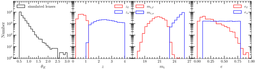
Figure 1: The distribution of the properties of the simulated lenses is constructed by simct. Left to right: the Einstein radius, $\theta_{E}$; the redshift, $z$; the i-band magnitude, $m_{i}$; and the ellipticity, $e$. The red and blue colours denote lens and source quantities, respectively.

The HSC-SSP Survey is an optical imaging survey conducted with the Hyper Suprime-Cam (HSC, Miyazaki et al., 2018; Komiyama et al., 2018; Kawanomoto et al., 2018; Furusawa et al., 2018; Huang et al., 2018; Coupon et al., 2018), a $1.7\deg^{2}$ field-of-view optical camera on the 8.2-meter Subaru telescope, which has a pixel scale of 0.168″/pixel. In this work, we use data products from the HSC-SSP Public Data Release 2 (henceforth “PDR2") Wide covering $\sim$ 800 deg² (Aihara et al., 2019) in gri bands out of a final survey area of 1400 deg². The median $5\sigma$ depths (for point sources) in $gri$ filters for the PDR2 Wide layer are 26.6, 26.2, and 26.2 mag, while the median seeings are 0.77″, 0.76″, and 0.58″, for $gri$, respectively. The PDR2 data is processed with hscPipe version 6 (Bosch et al., 2018). The combination of a large area and observation depth makes the data from the HSC-SSP Survey ideal for discovering new or unusual strong gravitational lenses (e.g., HSC J090429.75-010228.2; Jaelani et al., 2020a).

The photometric redshifts used in this work are determined using the mizuki algorithm (Tanaka, 2015). The robustness of the photometric redshifts is a function of galaxy redshift and brightness, and is quantified in terms of $\Delta z/(1+z_{\rm ref})$, where ${\rm{\Delta}}z\equiv|z-{z}_{\rm ref}|$ and $z_{\rm ref}$ is a reference redshift. The mizuki’s photometric redshifts measurement are most accurate at $0.2\lesssim z_{\rm phot}\lesssim 1.5$. A thorough explanation of mizuki’s application to the HSC-SSP data is presented in Tanaka et al. (2018). Since the HSC-SSP Survey footprint overlaps with the Sloan Digital Sky Survey (SDSS), we collect spectroscopic redshifts, whenever available, from the SDSS Data Release 16 (Ahumada et al., 2020) catalogues.

For our strong lens search, we select to be our parent sample galaxies in PDR2 Wide retrieved from the HSC CAS Search service based on their magnitude limit, stellar mass, and star formation rate. To be more specific, we select objects from tables that satisfy the following criteria:

• for pdr2_wide.forced

  1. isprimary is True

  2. [grizy]_pixelflags_edge is False

  3. [grizy]_pixelflags_interpolatedcenter is False

  4. [grizy]_pixelflags_crcenter is False

  5. [grizy]_cmodel_flag is False

  6. i_extendedness_value > 0.9

  7. ([ri]_cmodel_mag $-$ a_[ri]) < 28.0

  8. (z_cmodel_mag $-$ a_z) < 23.0

• for pdr2_wide.forced2

  1. [grizy]_sdsscentroid_flag is False

• pdr2_wide.meas

  1. [grizy]_inputcount_value > 0

• pdr2_wide.masks

  1. i_mask_pdr2_bright_objectcenter is False

• pdr2_wide.photoz_mizuki

  1. 0.2 < photoz_median < 1.2

  2. stellar_mass > 5.0e10

  3. (sfr / stellar_mass) < 1.0e-10.

We remove objects with saturated pixels and unreliable photometry, as well as probable stars, using criteria 2-11. We concentrate on finding lensed features among a set of galaxies based on the properties that make them possible lenses, as defined by criteria 12-14. The upper redshift and lower stellar mass bounds are a compromise between obtaining a sample of lenses as complete as possible and the need to find lenses with Einstein radius smaller than 1″. The lower redshift cut is introduced to avoid dealing with galaxies that are too bright for the detection of lensed features, which are typically faint. This query returns a total of 2 350 061 unique HSC objects. We use HSC $gri$ cutouts (64 pixels $\times$ 64 pixels, which is sufficient for galaxy-scale lenses) centred on the parent objects, which are retrieved from the PDR2 Image Cutout service.

3 Simulated Galaxy-Scale Lenses

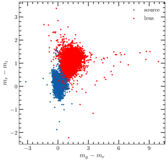
Figure 2: Distributions of color-color ($m_{r}-m_{i}$ vs. $m_{g}-m_{r}$) diagram of the lens galaxies (red), and the sources (blue).

In order to train the network on a large sample of realistic galaxy-scale lenses, we use the simct pipeline (detailed in More et al., 2016). With this pipeline, we superpose a set of simulated lensed galaxies on the real image cutouts of massive galaxies from the multi-band HSC imaging (see Section 2). This ensures that most of the features and properties in the training images will statistically be similar to the the real survey images which will be classified. The methodology of simct is summarized below.

The mass model of the lens galaxies is assumed to follow Singular Isothermal Ellipsoid (SIE, Kormann et al., 1994) and the contribution from an external shear is also included in the model (see Table 2). We start with the position, photometric magnitudes, photometric redshifts and ellipticity of the massive galaxies to convert their light parameters into the SIE model mass parameters. Thus, following the $L-\sigma_{v}$ scaling relation (Parker et al., 2005), we obtain the velocity dispersion. Similarly, assuming mass follows light, we obtain the position of the lens potential and the ellipticity parameters.

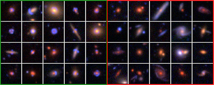
Figure 3: Green box: examples of simulated lenses based on real HSC SSP colour composite images. Red box: examples of objects used as non-lenses during the training of the CNN. All postage stamps are 64 pixels on-a-side, corresponding to 10.8″.

Table 2: Thresholds used in the selection of the simulated lenses.

Parameter	Range	Unit
Lens (SIE)
Einstein radius, $\theta_{E}$	[0.5, 3.0]	arcsec
Redshift, $z_{\ell,\rm phot}$	[0.2, 1.1]	-
External Shear, $\gamma_{\rm ext}$	[0.001, 0.020]
PA of External Shear, $\theta_{\gamma_{\rm ext}}$	[0, 180]	degree
Source
Redshift, $z_{s}$	[1.2, 4.0]	-
$i$-magnitude, $m_{i,s}$	[23, 26]	-
Ellipticity, $\theta_{e,s}$	[0.1, 0.8]	-
PA of Ellipticity, $\theta_{e,s}$	[0, 180]	degree

The $i$-band magnitude and the redshift of the background galaxies are drawn from the source counts and redshift distribution as prescribed in Faure et al. (2009). Faure et al. assumed that the number density of sources at redshift $z_{s}$ brighter than the apparent magnitude threshold of $m_{lim}\sim 26$ [mag] in the F814W filter band. Each galaxy is parameterised with a Sersic profile for a fixed Sersic index of 1 corresponding to an exponential profile. The ellipticity and position angle (PA) are drawn randomly from a uniform distribution within the range indicated in Table 2. The effective radius of the galaxy is estimated from the luminosity - size, $L-r_{\rm eff}$ relation (Bernardi et al., 2003, with a redshift scaling to account for size evolution). The colors of the galaxy are extracted from photometric CFHTLenS catalog (Hildebrandt et al., 2012; Erben et al., 2013).

We take into account the lensing optical depth to determine which massive galaxy is likely to act as a lens and accept a background source provided the Einstein radius falls within the range given in Table 2 and the magnitude of the second brightest lensed image is above the limiting magnitude of the HSC Survey (see More et al., 2016, for further details). Once all of the parameters for the lens and source models have been determined, we use gravlens (Keeton, 2001) to generate simulated lensed images. After accounting for the shot noise in the lensed images and convolving them with the seeing in each of the filters. The simulated lensed image is added to the real HSC image centred on the galaxy selected to act as a lens (see the left green box in Figure 3). Figure 1 shows the distributions of the Einstein radius, redshifts, $i$-band magnitude, and ellipticity for both lens and the source of the simulated galaxy-scale lenses. We also show the distribution of color-color ($m_{r}-m_{i}$ vs. $m_{g}-m_{r}$) diagram of the lens galaxies and the sources (see Figure 2) with selection effect tend to bluer sources.

From a total of about 22 000 simulated lens systems, we exclude about 3000 systems located within GAMA09H field which will be used for a comparison analysis in More et al. (2023, in prep.). We also exclude tens of simulated lens galaxies whose centres have been identified as known lens galaxies in previous studies (e.g., More et al., 2012; Sonnenfeld et al., 2018, 2020). We then end up with 18 660 simulated lens systems.

4 Convolutional Neural Network

The dataset for training the CNN is divided into two subsets of equal number of members: one containing the 18 660 simulated lenses simulated with 64 $\times$ 64 pixel (corresponding to 10.752″$\times$ 10.752″) cutouts from Section 3, and the other containing the 18 660 non-lens objects that were not used to generate simulated lenses. These cutouts are large enough to capture galaxy-scale lenses and yet small enough for fairly quick training and searching.

Table 3: Details of training and test samples used in the analyses.

Training Sample	Lenses	14 928
	Non-Lenses	14 928
Validation Sample	Lenses	3 732
	Non-Lenses	3 732
Test Sample	Lenses	220
	Non-Lenses	78 665
Composition of the Non-lens sample
Non-Lenses used in Training	Random Galaxies	55%
	Spiral Galaxies	34%
	Stars (SDSS Spectroscopic star)	5%
	Groups or LRG + edge-on galaxies	4%
	Doubles, ’tricky’ spirals or mergers	2%

Note:See Section 4 for further details.

Table 4: CNN Architecture

ID	Type	Size	$n$	Activation	Param Count
(1)	(2)	(3)	(4)	(5)	(6)
1	input	64 $\times$ 64	…	…	…
2	convolutional	11 $\times$ 11	64	ReLU	23 296
3	max pooling	2 $\times$ 2	…	…	…
4	convolutional	7 $\times$ 7	128	ReLU	401 536
5	dropout (0.2)	…	…	…	…
6	convolutional	5 $\times$ 5	128	ReLU	409 728
7	max pooling	2 $\times$ 2	…	…	…
8	convolutional	5 $\times$ 5	256	ReLU	819 456
9	dropout (0.2)	…	…	…	…
10	convolutional	3 $\times$ 3	256	ReLU	590 080
11	max pooling	2 $\times$ 2	…	…	…
12	fully-connected	1 024	…	ReLU	2 360 320
13	dropout (0.2)	…	…	…	…
14	fully-connected	1 024	…	ReLU	1 049 600
15	dropout (0.2)	…	…	…	…
16	fully-connected	512	…	ReLU	524 800
17	dropout (0.2)	…	…	…	…
18	fully-connected	512	…	ReLU	262 656
19	fully-connected	1	…	sigmoid	513
Total params:			6 441 985
Trainable params:			6 441 985
Nontrainable params:			0

Notes. (1) ID of the layers. (2) Type of the layers. (3) Size of the data or the filters. (4) Number of the filters. (5) Activation function adopted in the layers. (6) Trainable parameters.

The dataset is split into 80% for training and 20% for validation (see Table 3). We select non-lens objects for the negatives, which contains: 55% galaxies that are randomly selected from the parent catalogue; 34% spiral galaxies from Tadaki et al. (2020); 5% stars from the SDSS spectroscopic star catalogue (Ahumada et al., 2020); 4% galaxy groups or "crowded" galaxies like LRG + egde-on galaxy (or arc like feature); and 2% dual point-like, tricky spiral or merger galaxies that are visually inspected from the parent catalogue (see the right red box in Figure 3).

In order to identify blue sources, we select HSC $gri$-band images due to their excellent depth and quality. The FITS images in three bands are converted to RGB images scaled with an arcsinh stretch using HumVI (Marshall et al., 2016) and supplied to the CNN as vectors of 12 288 (64 $\times$ 64 $\times$ 3) floating-point numbers. Before the CNN’s training stage, we preprocess our data by normalizing each image brightness to be between 0 and 1. In general, data augmentation is a common practise in machine learning; it is used to expand the training set in order to prevent overfitting and teach the network rotational, translational and scaling invariance. Here, we use in-place data augmentation to make sure that, when the network is trained, it sees new variations of our dataset at each and every epoch. This augmentation method is done at training time and not an "additive" operation which is transforming the original data in the batch by a series of random transformation, then returning the randomly transformed into network for training. We augment our dataset applying the following transformations to the simulated and non-lens galaxy sample: (i) a random rotation in the range [-30 deg, 30 deg]; (ii) a random resizing by a factor in the range [0.8, 1.2]; (iii) a random flip along the horizontal axis; (iv) and a random channel_shift_range $=0.9$.

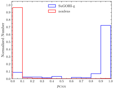
Figure 4: Histogram of the probabilities predicted by the trained CNN for all lens and non-lens of test sample.

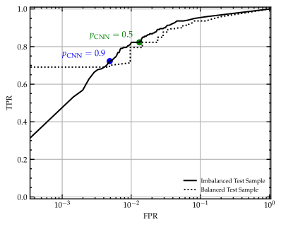
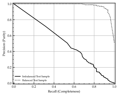
Figure 5: Top: Receiver Operating Characteristic curves for the trained CNN showing the true position rate (TPR) as function of the false positive rate (FPR) for different lens identification thresholds. The corresponding area under curve (AUC) are 0.976 and 0.971, for imbalanced and balanced test sample, respectively. Bottom: Precision-Recall (PR) curves for the trained CNN showing the precision as function of the recall. Note that this performances describes a test dataset with a 50-50 split (for balanced) and a 0.3-99.7 split (for imbalanced) between lens and non-lens containing images. Number of test sample is shown in Table 5.

The CNN architecture is inspired by LeNet (Lecun et al., 1998) and Jacobs et al. (2017), with modifications displayed in Table 4. The CNN consists of five convolutional layers with kernel sizes of 11 $\times$ 11, 7 $\times$ 7, 5 $\times$ 5, 5 $\times$ 5, and 3 $\times$ 3; 64, 128, 128, 256, and 256 filters, followed by four fully connected hidden layers with 1 024, 1 024, 512, and 512 neurons. Five dropout regularizations (Srivastava et al., 2014) are performed in between convolutional and fully-connected layers to minimise the likelihood of overfitting by dropping 20% of the output neurons at random during training with Rectified Linear Unit (ReLU; Nair & Hinton, 2010) nonlinear activations. The output layer consists of a single neuron with sigmoid activation. Three Maxpooling layers with $2\times 2$ kernel sizes and stride 2 are inserted between the convolutional layers to make the CNN invariant to local translations of the relevant features in gri image cutouts while reducing the network parameters. The network has a total of 6 441 985 trainable parameters upon completion. The network is summarised in Table 4.

We use the Adam optimization algorithm (Kingma & Ba, 2014) to minimise the cross-entropy error function over the training data with a learning rate of 0.00005. The CNN is trained for 100 epochs using mini-batch stochastic gradient descent with 128 images per batch. If the network does not provide improved accuracy or loss after five consecutive epochs, we terminate the training early. This network is implemented utilising the Python neural network library Keras (Chollet & others, 2018) with the TensorFlow backend (Abadi et al., 2016).

Completeness is measured on spectroscopically-confirmed or grade A or B SuGOHI galaxy-scale lenses (Sonnenfeld et al., 2018; Wong et al., 2018; Sonnenfeld et al., 2020). We rejected a few lenses with large image separations $\gtrsim 3\arcsec$, indicating significant perturbation from the lens environment, as we have no intention of recovering such configurations. As test lenses, we use 220 SuGOHI-g lens systems. We collect the 78 665 non-lenses, including random galaxies from a parent catalogue; spiral galaxies from Tadaki et al. (2020); and stars from the SDSS spectroscopic star catalogue (Ahumada et al., 2020).

4.1 CNN Performance

The CNN provides a score, $p_{\rm CNN}$, ranging from 0 to 1, with 1 for lenses and 0 for everything else (non-lenses). The evolution of the training and validation loss for the network with optimised hyperparameters until epoch 52, which corresponds to the validation set’s minimal binary cross-entropy loss without overfitting. The network achieved a training (validation) accuracy of 0.986 (0.981) and a loss of 0.041 (0.059). The small difference between the two curves (generalisation gap) indicates that the model’s predictions on new data with similar properties to the training set are relatively stable. Using the test set, the final network performance was characterised. In Figure 4, we show the probabilities predicted by the model for all lens and non-lens test examples. When $p_{\rm CNN}>0.9$, the distribution is dominated by lenses.

To evaluate the number of lenses correctly identified, we use a Receiver Operating Characteristic (ROC) curve which compares the True Positive Rate (TPR) to the False Positive Rate (FPR) as functions of the decision threshold applied to the score and Precision-Recall (PR) curves for the trained CNN showing the precision as function of the recall or TPR. In general, the excellent performance are shown by the ROC and PR curves in Figure 5. The ROC curve illustrates the performance of a binary classifier in distinguishing between the two classes as the decision threshold is altered. The Area Under the ROC Curve (AUC) of our CNN are 0.976 and 0.971, for imbalanced (0.3-99.7) and balanced (50-50) test sample, respectively. For balanced test sample, the PR curve shows that the network can classifies all objects as lens sample would yield a precision (purity) of 97.3% at a recall (completeness) of 82.3% of SuGOHI-g lenses in the test set with an FPR of 1.3% for $p_{\rm CNN}=0.5$ as the threshold; and a precision of 98.8% at a recall of 72.3% of SuGOHI-g lenses with an FPR of 0.49% for $p_{\rm CNN}=0.9$ as a threshold (see Table 5).

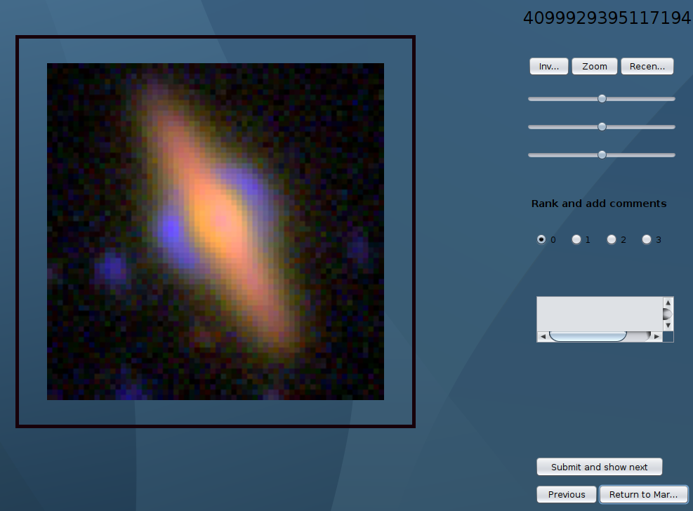
Figure 6: Example of an image cutout as viewed on the visapp. The cutout is 10.752″on a side.

4.2 Visual Inspection

We applied the trained CNN to the $gri$ cutouts of all 2.4 million galaxies in order to determine their score $p_{\rm CNN}$. The CNN identifies 55 469, 20 241, and 1830 as candidate lenses with $p_{\rm CNN}>0.5$, $p_{\rm CNN}>0.9$, and $p_{\rm CNN}=1.0$, respectively. About 0.86% of the parent sample has $p_{\rm CNN}>0.9$. We note that several candidates have a blue feature close to a red galaxy with a very faint or no counter blue image. This is possibly due to our training dataset being sensitive to small Einstein radii. After an initial visual inspection performed by a single inspector (ATJ) to remove definite non-lenses, a "good" sample of 1522 potential lens candidates is determined.

We inspect RGB images of these candidates using visapp, which displays PNG images made with $gri$ imaging using three different scaling parameters. Figure 6 illustrates a sample page of candidates from the visapp. We assign each candidate a grade between 0 and 3, using the grading convention from Sonnenfeld et al. (2020), where 0 means "almost certainly not a lens", 1 means "possibly a lens", 2 means "probably a lens", and 3 means "almost certainly a lens". There are comment columns for the candidates that require further discussion. It is possible to invert the images’s colour, zoom in or out and shift it. The grades used throughout the paper are the mean grade, $\langle Gr\rangle$, assigned by authors ATJ, AM, KTI, DCYC, KCW, and PWP.

Table 5: Results of the lens search on the parent catalogue.

Criteria	Number
Image tested	2 350 061
First candidates set
$p_{\rm CNN}>0.5$	55 469
$p_{\rm CNN}>0.9$	20 241
$p_{\rm CNN}=1.0$	1 830
Second candidates set	1 522
Final candidates set	1 292
Grade A	43
Grade B	269
Known (A or B)	215
New (A or B)	97
Grade C	880
Known (C)	289
For balanced test sample (50-50)
Precision (purity)
($p_{\rm CNN}>0.5$)	97.3%
($p_{\rm CNN}>0.9$)	98.8%
Recall (completeness)
($p_{\rm CNN}>0.5$)	82.3%
($p_{\rm CNN}>0.9$)	72.3%
For imbalanced test sample (0.3-99.7)
Precision (purity)
($p_{\rm CNN}>0.5$)	14.9%
($p_{\rm CNN}>0.9$)	29.3%
Recall (completeness)
($p_{\rm CNN}>0.5$)	82.3%
($p_{\rm CNN}>0.9$)	72.3%
The fraction of grades A and B with $\langle Gr\rangle>1.5$
$0.95<p_{\rm CNN}\leq 1.00$	268/312
$0.90<p_{\rm CNN}\leq 0.95$	44/312

Next, we implemented the scheme outlined below (Sonnenfeld et al., 2018):

1. A: $\langle Gr\rangle>2.5$,

2. B: $1.5<\langle Gr\rangle\leq 2.5$,

3. C: $0.5<\langle Gr\rangle\leq 1.5$, and

4. Not a lens: $\langle Gr\rangle\leq 0.5$.

Then, the grades were compiled and averaged, and each grader’s scores were revealed and compared. Graders were then allowed to adjust their scores, particularly for contentious objects with disparate scores or scores close to the grade thresholds. During this stage, we also used the HSC PDR2 map for additional inspection, if necessary.

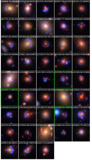
Figure 7: Images for the 43 lens candidates with grades A. All images are oriented with North up and East left. Green boxes indicate newly discovered candidates.

Table 6: The grade A and B strong lens candidates. Column 1 is ID of the system name. Columns 2 and 3 are right ascension and declination of the lens galaxy. Columns 4 and 5 are the i-band CModel magnitude and photometric redshift of the lens galaxy provided by the HSC catalogue. Columns 6 gives the spectroscopic redshifts of the lens galaxy inferred from SDSS DR16. Column 7 is the CNN score. Column 8 is the average visual-inspection score of the lens system. ’This Work’ indicates a completely new discovery. Other relevant references in column 9 are:(a) Sonnenfeld et al. (2018), (b) Wong et al. (2018), (c) Sonnenfeld et al. (2019), (d) Chan et al. (2020), (e) Jaelani et al. (2020b), (f) Sonnenfeld et al. (2020), (g) More et al. (2012), (h) More et al. (2016), (i) Petrillo et al. (2019), (j) Huang et al. (2020), (k) Cañameras et al. (2020), (l) Cañameras et al. (2021), (m) Jacobs et al. (2019), (n) Cabanac et al. (2007), (o) Faure et al. (2008), (p) Gavazzi et al. (2014), (q) Li et al. (2020), (r) Brownstein et al. (2012), (s) Shu et al. (2016), (t) Shu et al. (2022), (u) Wong et al. (2022). The full list is available at the http://www-utap.phys.s.u-tokyo.ac.jp/$\sim$oguri/sugohi/.

HSC_ID	$\alpha$(J2000)	$\delta$(J2000)	$m_{i,\ell}$	$z_{\ell,\rm phot}$	$z_{\ell,\rm spec}$	PCNN	$\langle Gr\rangle$	References
J000848.79+001550.8	2.20333	0.26412	19.57	0.348	0.397	0.901	2.667	e, l, t
J015310.58-042315.5	28.29412	-4.38766	19.01	0.306	…	0.990	2.667	t
J015731.49-033057.6	29.38125	-3.51603	17.83	0.683	0.621	1.000	2.667	a, l, t
J020517.00-012320.4	31.32086	-1.38901	19.57	0.770	…	0.997	2.667	l, m
J021411.22-040502.8	33.54676	-4.08411	17.99	0.662	0.609	0.987	2.667	b, e, g, l, n, p, t
J021737.15-051329.4	34.40481	-5.22486	17.96	0.629	0.646	0.996	3.000	c, e, m, n, p, t
J022610.67-042011.6	36.54447	-4.33658	18.57	0.469	0.495	0.991	2.667	a, c
J023637.30-033220.1	39.15545	-3.53893	20.03	0.275	0.269	1.000	3.000	a, e, l, t
J023817.77-054555.5	39.57404	-5.76543	20.13	0.594	0.599	0.999	3.000	a, c, d, l
J085046.60+003905.4	132.69420	0.65150	20.98	0.951	…	0.988	3.000	f, l, t
J090407.93-005953.0	136.03306	-0.99807	18.77	0.622	…	1.000	3.000	g, l, n, t
J091904.60+033638.5	139.76917	3.61072	20.28	0.406	0.444	0.963	2.833	a, e, k, l, t
J092544.99+001702.8	141.43748	0.28413	20.42	0.840	…	0.908	3.000	e, f, l, t
J094123.03+000446.6	145.34596	0.07964	21.28	0.456	0.486	1.000	2.667	b, l, t
J115315.59+012745.8	178.31498	1.46274	20.09	0.504	…	1.000	2.833	e, f, t
J115653.02-003948.5	179.22093	-0.66350	21.31	0.540	0.508	0.991	2.667	a, i, t
J120611.66-010407.2	181.54861	-1.06867	18.18	0.534	…	0.997	2.833	l, t
J121052.47-011905.2	182.71866	-1.31814	21.26	0.683	0.700	0.998	2.667	a, c, d, l, t
J121504.44+004726.0	183.76850	0.79057	20.32	0.655	0.642	1.000	2.667	c, r
J122314.74-002939.5	185.81143	-0.49432	18.26	0.541	0.547	0.990	2.667	b, l, t
J122456.00+005047.9	186.23336	0.84665	17.98	0.226	…	0.996	2.667	l, q
J124320.77-004517.7	190.83655	-0.75494	18.23	0.634	0.654	0.938	2.667	b, i, l, t
J141136.51-010215.6	212.90214	-1.03769	20.96	0.993	0.949	1.000	3.000	d, f
J141236.23+423339.7	213.15097	42.56105	20.01	0.854	…	0.996	2.667	This Work
J141300.06-012608.1	213.25027	-1.43561	20.81	0.757	0.749	0.999	2.667	a, c, d, l
J141624.21-002101.2	214.10091	-0.35036	20.18	0.631	…	0.981	2.667	This Work
J141649.81+013822.2	214.20756	1.63951	20.02	0.313	…	1.000	2.667	f, i, l, t
J142720.54+001916.0	216.83560	0.32111	17.32	0.558	0.551	0.981	2.833	a, c, l, t
J143438.07+431542.1	218.65864	43.26171	20.04	0.342	0.385	0.998	2.833	e, l, t
J143454.39-005658.6	218.72664	-0.94964	18.36	0.729	0.728	0.948	2.667	a, e, t
J144320.63-012537.2	220.83598	-1.42700	18.83	0.952	0.890	0.983	2.667	d, f
J145236.65-002142.1	223.15272	-0.36171	18.15	0.695	0.733	0.997	2.667	a, l, t
J151336.77+433250.9	228.40322	43.54750	20.85	0.469	0.487	0.968	2.667	b, l, t
J151833.93+430702.5	229.64140	43.11739	19.90	0.986	…	0.941	2.667	This Work
J155517.74+415138.6	238.82392	41.86074	20.34	0.600	0.555	1.000	2.667	a, k, l, t
J223733.54+005015.6	339.38976	0.83767	19.97	0.634	0.605	0.986	2.667	a, c, t
J223934.68+023507.4	339.89453	2.58540	17.41	0.981	…	0.961	2.667	e, f, t
J224614.61+055828.5	341.56090	5.97459	20.00	0.274	0.340	0.957	3.000	e, l, t
J224842.56+052217.7	342.17737	5.37159	20.21	0.904	…	0.920	2.667	t
J224932.75+031114.4	342.38647	3.18736	20.36	0.315	…	0.998	3.000	l, t
J230521.66-000211.6	346.34029	-0.03658	20.27	0.497	0.492	1.000	3.000	b, l, m, t
J233130.47+003733.4	352.87700	0.62595	20.11	0.535	0.552	1.000	2.833	b, l, m, t
J234117.53-002937.9	355.32304	-0.49388	18.99	0.511	0.531	0.979	2.833	l, t, u
J000326.35-002140.8	0.85980	-0.36133	18.34	0.794	…	1.000	1.667	This Work
J001313.60+002759.9	3.30668	0.46665	18.95	0.542	…	0.990	1.667	t
J011219.08-001539.3	18.07951	-0.26094	20.63	0.541	…	0.985	1.667	This Work
J011225.76-002247.0	18.10737	-0.37974	21.50	0.476	0.466	0.990	2.167	e
J012204.59-002222.1	20.51915	-0.37282	20.78	1.036	0.848	0.989	1.667	This Work
J012402.54-004559.3	21.01060	-0.76648	20.02	0.537	0.543	0.964	1.667	t
J015702.39-053436.0	29.25998	-5.57669	19.39	0.319	…	0.936	2.500	This Work
J015713.94-045446.9	29.30809	-4.91304	21.41	0.774	…	0.993	1.833	This Work
J020832.14-043315.8	32.13393	-4.55439	19.30	0.761	…	0.988	2.000	e, h, l, t
J095906.48+024524.8	149.77704	2.75691	19.37	0.317	0.346	0.954	1.833	o
J115944.63-000728.2	179.93600	-0.12452	20.92	0.734	0.332	0.988	2.333	r
J232557.38-005226.8	351.48909	-0.87412	20.11	0.794	…	0.980	2.167	j, l, m
J234248.68-012032.6	355.70284	-1.34239	18.00	0.578	0.527	0.998	2.000	l, s
⋮	⋮	⋮	⋮	⋮	⋮	⋮	⋮	⋮

5 Results

In total, we discover 43 grade A, 269 grade B, and 880 grade C candidates. The results are summarised in Table 5, which include the number of parent sample, lens candidates, purity, and completeness. The full list of the grade A and some examples of grade B candidates are given in Table 6. We note that the nearby lensed arcs could affect the $i$-band magnitude and photometric redshift. We show colour composite images of the grade A candidates in Figure 7 and of the grade B candidates in Figure 9. The lens redshift distribution of the grade A and grade B candidates is shown in Figure 8 with the peak at $z_{\ell,\ \rm{phot}}\sim 0.7$ and $z_{\ell,\ \rm{spec}}\sim 0.6$. While some lens candidates which were grade C from previous SuGOHI publications have been upgraded to a higher grade in recent references, we list the grade C lens candidates in the Appendix. The fraction of grades A and B with $\langle Gr\rangle>1.5$ among CNN recommendations, decreases rapidly when lowering the threshold $p_{\rm CNN}$. We estimate that 85.9% of the highest scores $0.95<p_{\rm CNN}\leq 1.00$ which has $\langle Gr\rangle>1.5$, and about 14.1% for $0.90<p_{\rm CNN}\leq 0.95$. In general, we find that the majority of lensed sources have a blue colour, which is due to the selection effect from our training sample.

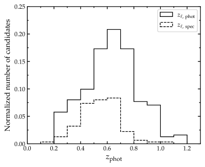
Figure 8: Histogram of lens redshifts for the combined grade A and grade B candidates found in this study.

Separately from this work, Cañameras et al. (2021) and Shu et al. (2022) have recently applied machine-learning-based lens search algorithms to the HSC-SSP PDR2 (Aihara et al., 2019) and have published lens candidates from these searches. Our parent sample and training set have smaller number of galaxies compared to Cañameras et al. (2021) and Shu et al. (2022), however, we still are able to discover a comparable number of lenses (see details in More et al. in prep). We noted that about 51 percent of our parent sample and the parent sample from Cañameras et al. (2021) overlapped. There is some overlap in the candidates we discovered as we used the HSC-SSP dataset. We have identified and cross-matched previous candidates with our candidates and listed the relevant references in Table 6. We find 504 overlapping candidates with 215 and 289 candidates from grade A or B, and grade C, respectively. We find that 143 of 289 overlapping grade C have a higher grade in previous searches. Our CNN also recovers 32 group- and cluster-scale lens candidates, although it is not optimized for these systems. Many candidates with a blue arc feature near a red galaxy have a lower grade, as seen in Table 12. Rojas et al. (2023) found that is difficult for experts to recover candidates with Einstein radius less than 1.2 times the seeing during visual inspection.

6 Summary

We present new candidates for galaxy-scale strong gravitational lenses from the HSC-SSP PDR2, covering 800 deg² in the $gri$ bands, using a CNN as part of the SuGOHI project. In order to identify possible galaxy-scale lenses, we use strict pre-selection criteria, such as multiband magnitudes, stellar mass, star formation rate, extendedness limit, and photometric redshift range, resulting in about 2.4 million galaxies of parent sample. By initially adopting a conventional threshold, $p_{\rm CNN}>0.9$, we find 20 241 candidates which are then refined to 1 522 systems with lensing features for further inspection.

On the basis of visual inspections of the cutouts, six authors independently graded the strong lens candidates. According to the average visual inspection scores, 312 candidates identified by the CNN are considered grade A or B (i.e., definite or probable), and 880 are grade C (possible) strong-lens candidates. This list was cross-referenced with our extensive compilation of strong gravitational lenses previously published as confirmed systems or candidates in order to identify duplicates. Among the candidates, there are 97 new discoveries (3 from grade A and 94 from grade B, respectively). We find that 143 grade C candidates were graded as A or B in previous literature. The (photometric) redshift of the candidate lens galaxies range from 0.2 to 1.2. Follow-up spectroscopy will confirm these lenses and measure source redshifts so that detailed lens modelling can yield scientific results.

Data Availability

The basic information of the lens candidates can be browsed or downloaded from the SuGOHI online database http://www-utap.phys.s.u-tokyo.ac.jp/~oguri/sugohi/ and imaging data from the HSC-SSP Public Data Release 2 https://hsc-release.mtk.nao.ac.jp/doc/.

Appendix A Images of 269 Grade B Candidate

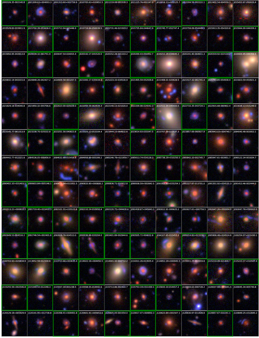
Figure 9: Images for the 269 lens candidates with grades B. All images are oriented with North up and East left. Green boxes indicate the new ones.

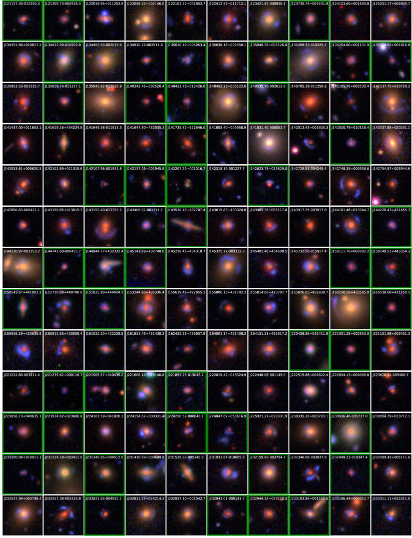
Figure 10: Continued.

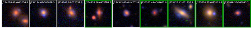
Figure 11: Continued.

Appendix B Images of 143 Grade C Candidate

The full list of 880 grade C is also available at the http://www-utap.phys.s.u-tokyo.ac.jp/$\sim$oguri/sugohi/. Here we show 143 grade C candidates which had higher grade in previous references.

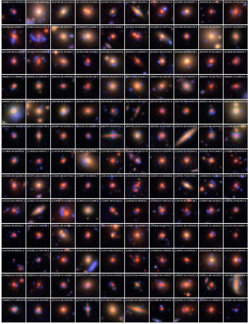
Figure 12: Images for the 143 lens candidates with grades C. All images are oriented with North up and East left.

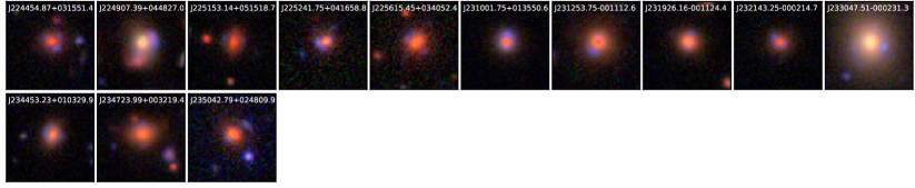
Figure 13: Continued.

References

- Abadi et al. (2016) Abadi M., et al., 2016, arXiv e-prints, p. arXiv:1603.04467
- Ahumada et al. (2020) Ahumada R., et al., 2020, ApJS, 249, 3
- Aihara et al. (2019) Aihara H., et al., 2019, PASJ, 71, 114
- Allingham et al. (2023) Allingham J. F. V., et al., 2023, MNRAS, 522, 1118
- Astropy Collaboration et al. (2013) Astropy Collaboration et al., 2013, A&A, 558, A33
- Astropy Collaboration et al. (2018) Astropy Collaboration et al., 2018, AJ, 156, 123
- Auger et al. (2010) Auger M. W., Treu T., Bolton A. S., Gavazzi R., Koopmans L. V. E., Marshall P. J., Moustakas L. A., Burles S., 2010, ApJ, 724, 511
- Bernardi et al. (2003) Bernardi M., et al., 2003, AJ, 125, 1866
- Birrer et al. (2020) Birrer S., et al., 2020, A&A, 643, A165
- Bosch et al. (2018) Bosch J., et al., 2018, PASJ, 70, S5
- Brownstein et al. (2012) Brownstein J. R., et al., 2012, ApJ, 744, 41
- Cañameras et al. (2020) Cañameras R., et al., 2020, A&A, 644, A163
- Cañameras et al. (2021) Cañameras R., et al., 2021, A&A, 653, L6
- Cabanac et al. (2007) Cabanac R. A., et al., 2007, A&A, 461, 813
- Caswell et al. (2019) Caswell T. A., et al., 2019, matplotlib/matplotlib v3.1.0, Zenodo, doi:10.5281/zenodo.2893252
- Chan et al. (2015) Chan J. H. H., Suyu S. H., Chiueh T., More A., Marshall P. J., Coupon J., Oguri M., Price P., 2015, ApJ, 807, 138
- Chan et al. (2020) Chan J. H. H., et al., 2020, A&A, 636, A87
- Chan et al. (2024) Chan J. H. H., et al., 2024, MNRAS, 527, 6253
- Chollet & others (2018) Chollet F., others 2018, Keras: The Python Deep Learning library (ascl:1806.022)
- Coupon et al. (2018) Coupon J., Czakon N., Bosch J., Komiyama Y., Medezinski E., Miyazaki S., Oguri M., 2018, PASJ, 70, S7
- Developers (2022) Developers T., 2022, TensorFlow, Zenodo, doi:10.5281/zenodo.4724125
- Erben et al. (2013) Erben T., et al., 2013, MNRAS, 433, 2545
- Faure et al. (2008) Faure C., et al., 2008, ApJS, 176, 19
- Faure et al. (2009) Faure C., et al., 2009, ApJ, 695, 1233
- Furusawa et al. (2018) Furusawa H., et al., 2018, PASJ, 70, S3
- Gavazzi et al. (2014) Gavazzi R., Marshall P. J., Treu T., Sonnenfeld A., 2014, ApJ, 785, 144
- Gilman et al. (2020) Gilman D., Birrer S., Nierenberg A., Treu T., Du X., Benson A., 2020, MNRAS, 491, 6077
- Harris et al. (2016) Harris D. W., et al., 2016, AJ, 151, 155
- Hezaveh et al. (2016) Hezaveh Y. D., et al., 2016, ApJ, 823, 37
- Hildebrandt et al. (2012) Hildebrandt H., et al., 2012, MNRAS, 421, 2355
- Hsueh et al. (2020) Hsueh J. W., Enzi W., Vegetti S., Auger M. W., Fassnacht C. D., Despali G., Koopmans L. V. E., McKean J. P., 2020, MNRAS, 492, 3047
- Huang et al. (2018) Huang S., et al., 2018, PASJ, 70, S6
- Huang et al. (2020) Huang X., et al., 2020, ApJ, 894, 78
- Huang et al. (2021) Huang X., et al., 2021, ApJ, 909, 27
- Inoue et al. (2016) Inoue K. T., Minezaki T., Matsushita S., Chiba M., 2016, MNRAS, 457, 2936
- Inoue et al. (2023) Inoue K. T., Minezaki T., Matsushita S., Nakanishi K., 2023, ApJ, 954, 197
- Jacobs et al. (2017) Jacobs C., Glazebrook K., Collett T., More A., McCarthy C., 2017, MNRAS, 471, 167
- Jacobs et al. (2019) Jacobs C., et al., 2019, ApJS, 243, 17
- Jaelani et al. (2020a) Jaelani A. T., et al., 2020a, MNRAS, 494, 3156
- Jaelani et al. (2020b) Jaelani A. T., et al., 2020b, MNRAS, 495, 1291
- Jaelani et al. (2021) Jaelani A. T., et al., 2021, MNRAS, 502, 1487
- Jauzac et al. (2021) Jauzac M., Klein B., Kneib J.-P., Richard J., Rexroth M., Schäfer C., Verdier A., 2021, MNRAS, 508, 1206
- Kawanomoto et al. (2018) Kawanomoto S., et al., 2018, PASJ, 70, 66
- Keeton (2001) Keeton C. R., 2001, arXiv e-prints, pp astro–ph/0102340
- Kingma & Ba (2014) Kingma D. P., Ba J., 2014, arXiv e-prints, p. arXiv:1412.6980
- Komiyama et al. (2018) Komiyama Y., et al., 2018, PASJ, 70, S2
- Koopmans et al. (2006) Koopmans L. V. E., Treu T., Bolton A. S., Burles S., Moustakas L. A., 2006, ApJ, 649, 599
- Kormann et al. (1994) Kormann R., Schneider P., Bartelmann M., 1994, A&A, 284, 285
- Lecun et al. (1998) Lecun Y., Bottou L., Bengio Y., Haffner P., 1998, Proceedings of the IEEE, 86, 2278
- Li et al. (2020) Li R., et al., 2020, ApJ, 899, 30
- Li et al. (2021) Li R., et al., 2021, ApJ, 923, 16
- Limousin et al. (2009) Limousin M., et al., 2009, A&A, 502, 445
- Marques-Chaves et al. (2017) Marques-Chaves R., et al., 2017, ApJ, 834, L18
- Marshall et al. (2016) Marshall P. J., et al., 2016, MNRAS, 455, 1171
- Metcalf et al. (2019) Metcalf R. B., et al., 2019, A&A, 625, A119
- Miyazaki et al. (2018) Miyazaki S., et al., 2018, PASJ, 70, S1
- More et al. (2012) More A., Cabanac R., More S., Alard C., Limousin M., Kneib J. P., Gavazzi R., Motta V., 2012, ApJ, 749, 38
- More et al. (2016) More A., et al., 2016, MNRAS, 455, 1191
- More et al. (2017) More A., et al., 2017, MNRAS, 465, 2411
- Nair & Hinton (2010) Nair V., Hinton G. E., 2010, in ICML.
- Newman et al. (2013) Newman A. B., Treu T., Ellis R. S., Sand D. J., 2013, ApJ, 765, 25
- Nierenberg et al. (2017) Nierenberg A. M., et al., 2017, MNRAS, 471, 2224
- Oguri et al. (2012) Oguri M., Bayliss M. B., Dahle H., Sharon K., Gladders M. D., Natarajan P., Hennawi J. F., Koester B. P., 2012, MNRAS, 420, 3213
- Parker et al. (2005) Parker L. C., Hudson M. J., Carlberg R. G., Hoekstra H., 2005, ApJ, 634, 806
- Petrillo et al. (2019) Petrillo C. E., et al., 2019, MNRAS, 484, 3879
- Refsdal (1964) Refsdal S., 1964, MNRAS, 128, 307
- Rojas et al. (2023) Rojas K., et al., 2023, MNRAS, 523, 4413
- Shajib et al. (2021) Shajib A. J., Treu T., Birrer S., Sonnenfeld A., 2021, MNRAS, 503, 2380
- Shu et al. (2016) Shu Y., et al., 2016, ApJ, 824, 86
- Shu et al. (2022) Shu Y., Cañameras R., Schuldt S., Suyu S. H., Taubenberger S., Inoue K. T., Jaelani A. T., 2022, A&A, 662, A4
- Sonnenfeld et al. (2015) Sonnenfeld A., Treu T., Marshall P. J., Suyu S. H., Gavazzi R., Auger M. W., Nipoti C., 2015, ApJ, 800, 94
- Sonnenfeld et al. (2018) Sonnenfeld A., et al., 2018, PASJ, 70, S29
- Sonnenfeld et al. (2019) Sonnenfeld A., Jaelani A. T., Chan J., More A., Suyu S. H., Wong K. C., Oguri M., Lee C.-H., 2019, A&A, 630, A71
- Sonnenfeld et al. (2020) Sonnenfeld A., et al., 2020, A&A, 642, A148
- Srivastava et al. (2014) Srivastava N., Hinton G., Krizhevsky A., Sutskever I., Salakhutdinov R., 2014, Journal of Machine Learning Research, 15, 1929
- Tadaki et al. (2020) Tadaki K.-i., Iye M., Fukumoto H., Hayashi M., Rusu C. E., Shimakawa R., Tosaki T., 2020, MNRAS, 496, 4276
- Tanaka (2015) Tanaka M., 2015, ApJ, 801, 20
- Tanaka et al. (2018) Tanaka M., et al., 2018, PASJ, 70, S9
- Vegetti et al. (2010) Vegetti S., Koopmans L. V. E., Bolton A., Treu T., Gavazzi R., 2010, MNRAS, 408, 1969
- Vegetti et al. (2012) Vegetti S., Lagattuta D. J., McKean J. P., Auger M. W., Fassnacht C. D., Koopmans L. V. E., 2012, Nature, 481, 341
- Wong et al. (2018) Wong K. C., et al., 2018, ApJ, 867, 107
- Wong et al. (2020) Wong K. C., et al., 2020, MNRAS, 498, 1420
- Wong et al. (2022) Wong K. C., Chan J. H. H., Chao D. C. Y., Jaelani A. T., Kayo I., Lee C.-H., More A., Oguri M., 2022, arXiv e-prints, p. arXiv:2203.12805
- Zaborowski et al. (2023) Zaborowski E. A., et al., 2023, ApJ, 954, 68