Coupled Confusion Correction: Learning from Crowds with Sparse Annotations

Abstract

As the size of the datasets getting larger, accurately annotating such datasets is becoming more impractical due to the expensiveness on both time and economy. Therefore, crowd-sourcing has been widely adopted to alleviate the cost of collecting labels, which also inevitably introduces label noise and eventually degrades the performance of the model. To learn from crowd-sourcing annotations, modeling the expertise of each annotator is a common but challenging paradigm, because the annotations collected by crowd-sourcing are usually highly-sparse. To alleviate this problem, we propose Coupled Confusion Correction (CCC), where two models are simultaneously trained to correct the confusion matrices learned by each other. Via bi-level optimization, the confusion matrices learned by one model can be corrected by the distilled data from the other. Moreover, we cluster the “annotator groups” who share similar expertise so that their confusion matrices could be corrected together. In this way, the expertise of the annotators, especially of those who provide seldom labels, could be better captured. Remarkably, we point out that the annotation sparsity not only means the average number of labels is low, but also there are always some annotators who provide very few labels, which is neglected by previous works when constructing synthetic crowd-sourcing annotations. Based on that, we propose to use Beta distribution to control the generation of the crowd-sourcing labels so that the synthetic annotations could be more consistent with the real-world ones. Extensive experiments are conducted on two types of synthetic datasets and three real-world datasets, the results of which demonstrate that CCC significantly outperforms state-of-the-art approaches. Source codes are available at: https://github.com/Hansong-Zhang/CCC.

Introduction

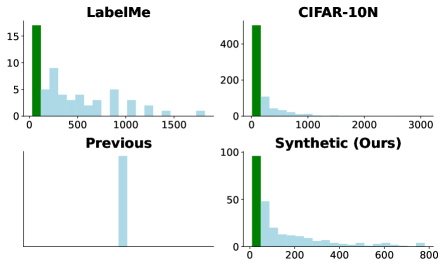
Figure 1: The histogram of the number of labels provided by annotators. The green patch on the left denotes the annotators who only provide seldom labels.

The great success of Deep Neural Networks (DNNs) is much attributed to large-scale and accurately-labeled training datasets. However, collecting such high-quality annotations demands the annotators to be experts in their discipline and is often very time-consuming (Song et al. 2023; Han et al. 2018; Zhang 2022). For instance, the well-known Microsoft COCO dataset were constructed using 20K work hours in total (Lin et al. 2014). To improve the efficiency of construct such datasets, crowd-sourcing (Biel and Gatica-Perez 2013; Buecheler et al. 2010; Han et al. 2019b; Servajean et al. 2017) provides an alternative way to collect annotations in a both time- and economic-efficient manner, where the labels of instances are provided by multiple annotators which could be non-expert. In the paradigm of crowd-sourcing, a large task is usually divided into several mini-tasks (one might overlap another), which will be further distributed to various annotators. On some crowd-sourcing platforms like Crowdflower (Wazny 2017) and Amazon Mechanical Turk, the annotators can get rewards when a mini-task is accomplished. Although crowd-sourcing is efficient in collecting large-scale annotations, it also inevitably introduces label noise (Sheng, Provost, and Ipeirotis 2008; Snow et al. 2008; Zheng et al. 2017), which is caused by the relatively-low expertise of some of the annotators. On the other hand, the DNNs can eventually memorize the noisy labels due to its great representative capacity (Zhang et al. 2021; Arpit et al. 2017; Ishida et al. 2020). Therefore, increasing the generalization performance of DNNs trained with crowd-sourcing annotations is a challenging problem, which is widely termed as Learning from Crowds (LFC).

In the discipline of LFC, previous solutions can be roughly divided into two pipelines: (1) Aggregate multiple noisy labels into a more reliable one before or during the training stage. Among them, the simplest one is Majority Voting (Whitehill et al. 2009; Han et al. 2019a; Schwenker 2013), where all the annotators are assumed to be equally reliable. Although Majority Voting provides a way to alleviate label noises, it is not always feasible to aggregate the labels equally, especially when the task is relatively hard and when most annotators are not reliable enough (Whitehill et al. 2009; Han et al. 2019a; Schwenker 2013). Motivated by that, some advanced methods were designed to model the expertise of each annotator. For instance, Weighted Majority Voting (Li et al. 2014) endows the labels with a weight vector to alleviate the influence of the annotators with low expertise. (2) Training under the supervision of all annotations. This pipeline of work usually take a set of confusion matrices as a measure of the expertise of annotators (Rodrigues and Pereira 2018; Dawid and Skene 1979; Chu, Ma, and Wang 2021; Wei et al. 2022a). By simultaneously learning the confusion matrices and the classifier in an end-to-end manner, these methods have achieved more promising performance in LFC compared to the label-aggregating ones (Rodrigues and Pereira 2018; Dawid and Skene 1979; Chu, Ma, and Wang 2021; Wei et al. 2022a; Li et al. 2023b).

Challenges. Despite their improved performance, the modeling of the expertise of annotators suffers from the following two problems, which will eventually jeopardises the performance of the classifier. On the one hand, Annotation Sparsity is a notorious property of the crowd-sourcing annotations (Ibrahim, Nguyen, and Fu 2023), which means that each annotator only labels a small subset of the whole dataset instead of all of it. On the other hand, the annotator-specific confusion parameters (ASCPs) (e.g. the weight vector or the confusion matrices in the aforementioned two pipelines) of each annotator are only learned based on its individual annotations. Therefore, if one annotator provides too few labels, it is obvious that the supervision of its ASCPs is insufficient and therefore its expertise can not be well-modeled (detailed analysis can be found in the Methodology Section). Note that such scenario is not hypothetical but quite ubiquitous. As shown in Figure 1, in real-world crowd-sourcing datasets LabelMe (Rodrigues and Pereira 2018) and CIFAR-10N (Wei et al. 2022b), a large number of annotators only provide seldom labels, even the authors of CIFAR-10N had enlarged the mini-tasks to alleviate annotation sparsity (Wei et al. 2022b).

To mitigate the sparse annotation problem in LFC, in this paper we propose Coupled Confusion Correction (CCC). In our CCC, two simultaneously-trained classifiers are coupled in a way where the confusion matrices learned by one classifier can be corrected by a small meta set (a class-balanced set that contains the images and their pseudo labels which are likely to be clean) distilled from the other one. Note that the labels in the meta set are actually from the crowd-sourcing labels. As the meta set has dropped the information of annotator IDs, it can not be directly used to supervise the learning of ASCPs. To this end, we link the meta set and ASCPs via meta learning, in which way each annotator’s ASCPs can be corrected by the meta set through bi-level optimization, even if the labels in meta set dose not come from him/her. Moreover, to further alleviate the annotation sparsity, we indicate and justify that there are many annotators who share similar expertise. Based on that founding, we use the K-Means method on the learned confusion matrices to cluster similar annotators so that their confusion matrices can be corrected together.

Our contributions can be summarized as follows:

$\bullet$ A Meta-Learning-Based Method CCC to Mitigate the Sparse Annotation Problem. In this work, we show that it is possible to learn one’s ASCPs under the supervision of other annotations except for its own individual ones. Specifically, we link the meta set and ASCPs through meta learning paradigm, so that the ASCPs can be corrected by the meta set, enriching its supervision. Moreover, we use K-Means to cluster annotators with similar expertise to further alleviate the annotation sparsity, correcting their ASCPs together.

$\bullet$ Synthetic More Practical Crowd-Sourcing Annotation using Beta Distribution. We point out a fact that is neglected by previous works: there exists some few-label annotators (annotators who only provide very few labels) in real-world crowd-sourcing datasets no matter how many the annotators are. To make our synthetic crowd-sourcing annotations more consistent with real-world ones, we propose to use Beta distribution to control the number of labels of each annotator. Previous works naively assumed that the amount of labels are evenly distributed, which may not accurately reflect real-world scenarios. Therefore, our proposed method is useful for future works on LFC when constructing synthetic annotations.

$\bullet$ Extensive and Comprehensive Experiments. We conduct experiments on various datasets, which include two types of synthetic crowd-sourcing datasets (independent and dependent cases) and three real-world datasets. The results demonstrate the competitiveness of our proposed method.

Methodology

Notations and Preliminaries. We begin by fixing notations. Suppose that we are given a training dataset $\tilde{\mathcal{D}}=\{\bm{x}_{i},\tilde{\bm{y}}_{i}\}_{i=1}^{N}$ which consists of $N$ instances labeled by $R$ annotators in total. Denote the data features as $\mathbf{x}=\{\bm{x}_{i}\}_{i=1}^{N}$ and the crowd-sourcing labels as $\mathbf{y}=\{\tilde{\bm{y}}_{i}\}_{i=1}^{N}$, where $\tilde{\bm{y}}_{i}=\left(\tilde{{y}}_{i}^{1},\tilde{{y}}_{i}^{2},...,\tilde{{y}}_{i}^{R}\right)$. The $i$-th crowd-sourcing label $\tilde{\bm{y}}_{i}$ is a $R$-dimensional vector representing the labels provided by $R$ annotators. Note that it is usually the case that an annotator does not label all the data, so the crowd-sourcing labels may have missing ones. Let $C$ denotes the number of class categories, then the individual label $\tilde{y}\in\{1,2,...,C\}$. The goal of learning from crowds is to train a classifier $f(\bm{x};\bm{\theta})$ parameterized by $\bm{\theta}$ (we take DNN as the classifier in this paper, which takes the instance feature $\bm{x}$ as input and outputs the possibility distribution over all classes) with training set $\tilde{\mathcal{D}}$, and to make it perform well on the unseen data.

Meta Learning Recap

Next, we will briefly recap the preliminaries on Meta Learning. In the meta-learning-based methods (Shu et al. 2019; Wang, Hu, and Hu 2020; Zheng, Awadallah, and Dumais 2021; Xu et al. 2021; Zhang and Pfister 2021), an out-of-sample meta set $\mathcal{D}^{meta}=\{\bm{x}^{meta}_{j},{y}_{j}^{meta}\}_{j=1}^{M}$ is assumed to be available, where $y_{j}^{meta}$ denotes the true label of the $j$-th meta data $\bm{x}^{meta}_{j}$ and $M(M\ll N)$ denotes the size of meta set. Note that the size of the meta set is much smaller than the training set, hence it is easy to collect in practice. The meta set can be either additionally provided (Shu et al. 2019; Wang, Hu, and Hu 2020; Zheng, Awadallah, and Dumais 2021) or distilled from the training set (Xu et al. 2021; Zhang and Pfister 2021). Various hyper-parameters (e.g. instanced by the transition matrix (Wang, Hu, and Hu 2020), label corrector net (Zheng, Awadallah, and Dumais 2021) or multi-layer perceptron network (Shu et al. 2019)) are called meta parameters and are updated via bi-level optimization, in which the meta set plays an important role in guiding the updating of such meta parameters. Intuitively, the performance of the current model on unseen data is measured by the meta set, the loss of the model on the meta set (termed as meta loss) is minimized in the outer loop of the bi-level optimization so that the gradient can flow back from the meta set to the meta parameters.

Typically, there are two sets of parameters to be optimized in such bi-level optimization, one is the aforementioned meta parameters, the other is the main parameters (mostly instanced by the parameters of the backbone model). Let $\bm{w}/\bm{\theta}$ denote the meta / main parameters, and $\mathcal{L}_{i}^{tra}(\bm{w},\bm{\theta})$ be the loss of the $i$-th instance in the training set $\tilde{\mathcal{D}}$. The optimal main parameters can be obtained by the training loss:

$$\bm{\theta}^{\star}(\bm{w})=\operatorname*{arg\,min}_{\bm{\theta}}\frac{1}{N}\sum_{i=1}^{N}\mathcal{L}_{i}^{tra}(\bm{w},\bm{\theta}).$$ (1)

Then the meta parameters can be optimized by minimizing the meta loss:

$$\bm{w}^{\star}=\operatorname*{arg\,min}_{\bm{w}}\frac{1}{M}\sum_{j=1}^{M}\mathcal{L}_{j}^{meta}(\bm{\theta}^{\star}(\bm{w})),$$ (2)

where the $\mathcal{L}_{j}^{meta}(\bm{\theta}^{\star}(\bm{w}))$ is the loss of the $j$-th instance in $\mathcal{D}^{meta}$. However, directly solving Eq. (1) and Eq. (2) is impractical, because the optimal $\bm{\theta}$ needs to be calculated whenever the meta parameters $\bm{w}$ is updated. Therefore, an online optimization method, as a trade-off between the feasibility and effectiveness, has been widely applied to the optimization of meta learning, which consists of three stages, including Virtual, Meta, and Actual stage (Wang, Hu, and Hu 2020). The optimization is performed in a mini-batch gradient descent manner, in $t$-th iteration, a training mini-batch $\tilde{\mathcal{M}}=\{\bm{x}_{i},\tilde{\bm{y}}_{i}\}_{i=1}^{n}$ and a meta mini-batch $\mathcal{M}^{meta}=\{\bm{x}^{meta}_{j},{y}^{meta}_{j}\}_{j=1}^{m}$ is fetched, where the $n$ and $m$ is the batch size of training and meta set respectively. Let $\eta_{v},\eta_{m},\eta_{a}$ denote the learning rates in the Virtual, Meta, and Actual stages respectively. In Virtual Stage, the main parameters is “virtually” updated by:

$$\hat{\bm{\theta}}_{t}=\bm{\theta}_{t-1}-\eta_{v}\frac{1}{n}\sum_{i=1}^{n}\nabla_{\bm{\theta}_{t-1}}\mathcal{L}_{i}^{tra}(\bm{w}_{t-1},\bm{\theta}_{t-1}).$$ (3)

This stage is named “virtual” because the true main parameters are kept unchanged, the above $\hat{\bm{\theta}}_{t}$ is fixed and only used to update the meta parameters in the following Meta stage:

$$\bm{w}_{t}=\bm{w}_{t-1}-\eta_{m}\frac{1}{m}\sum_{j=1}^{m}\nabla_{\bm{w}_{t-1}}\mathcal{L}_{j}^{meta}(\bm{w}_{t-1},\hat{\bm{\theta}}_{t}).$$ (4)

The Virtual stage, together with the Meta stage, can be deem as the outer loop of the bi-level optimization, which updates the meta parameters under the supervision of both meta set and training set (Wang, Hu, and Hu 2020). The “virtual” main parameters $\hat{\bm{\theta}}_{t}$ is deleted as soon as the Meta stage finished. Last, the $\bm{w}_{t}$ that comes from the outer loop will be fixed to update the main parameters in the Actual stage:

$$\bm{\theta}_{t}=\bm{\theta}_{t-1}-\eta_{a}\frac{1}{n}\sum_{i=1}^{n}\nabla_{\bm{\theta}_{t-1}}\mathcal{L}_{i}^{tra}(\bm{w}_{t},\bm{\theta}_{t-1}).$$ (5)

Unlike Virtual stage, the main parameters in this stage is “actually” updated. After the above three stages, both the main and meta parameters are updated and ready for the $(t+1)$-th iteration. Note that the Actual stage serves as the inner loop of the bi-level optimization. By alternating the outer and inner loop, the optimal main and meta parameters can be derived.

How Annotation Sparsity Affects Training

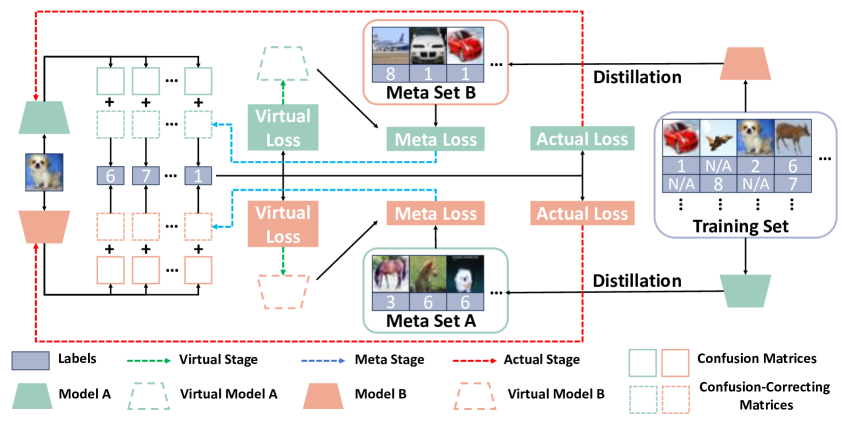
Figure 2: The illustration of the our method. “N/A” means the label is missing.

In this section, we would like to show why the sparse annotation phenomenon is harmful, which motivates our work. For notation convenience, we use a matrix $\mathcal{A}_{(N\times R)}$ to indicate the annotation presence, i.e., $\mathcal{A}_{i,j}$ is True if the $i$-th instance is labeled by $j$-th annotator, and False otherwise. Without loss of generality, we hereby take CrowdLayer (Rodrigues and Pereira 2018) as an example, which uses $R$ confusion matrices $\{\bm{T}^{r}\}_{r=1}^{R}$ to model the annotator-specific expertise. In CrowdLayer, the parameters of backbone DNN $\bm{\theta}$ and confusion matirces $\{\bm{T}^{r}\}_{r=1}^{R}$ are obtained by computing the following loss:

$$\bm{\theta}^{\star},\{\bm{T}^{r\star}\}_{r=1}^{R}=\operatorname*{arg\,min}_{\bm{\theta},\{\bm{T}^{r}\}_{r=1}^{R}}\frac{1}{N}\sum_{i=1}^{N}\sum_{r=1}^{R}\mathds{1}[\mathcal{A}_{i,r}]\mathcal{L}_{i,r}(\bm{T}^{r},\bm{\theta}),$$ (6)

where $\mathds{1}[\cdot]$ denotes the indicator function, which outputs $1$ if the event is True, and $0$ otherwise. $\mathcal{L}_{i,r}(\bm{T}^{r},\bm{\theta})=\ell(\bm{T}^{r}f(\bm{x}_{i}|\bm{\theta}),\tilde{y}^{r}_{i})$ stands for the loss of $i$-th instance and $r$-th annotator in CrowdLayer, where $\ell$ is a loss function such as widely-used cross entropy and $f$ is the softmax output of the classifier. For the $r_{0}$-th confusion matrix $\bm{T}^{r_{0}}$ (i.e. the ASCPs of $r_{0}$-th annotator), by modifying Eq. (6), the gradient w.r.t. $\bm{T}^{r_{0}}$ (denoted by $\bm{g}^{r_{0}}$) can be derived as:

$$\bm{g}^{r_{0}} =\nabla_{\bm{T}^{r_{0}}}\frac{1}{N}\sum_{i=1}^{N}\sum_{r=1}^{R}\mathds{1}[\mathcal{A}_{i,r}]\mathcal{L}_{i,r}(\bm{T}^{r},\bm{\theta})$$ (7)

$$=\nabla_{\bm{T}^{r_{0}}}\frac{1}{N}\sum_{i=1}^{N}\mathds{1}[\mathcal{A}_{i,r_{0}}]\mathcal{L}_{i,r_{0}}(\bm{T}^{r_{0}},\bm{\theta}),$$

from which we notice that only the instances labeled by $r_{0}$-th annotator provide supervised information to its own confusion matrix, let alone the labels could be noisy. Therefore, if $r_{0}$-th annotator labels too few data, its confusion matrix would be poorly learned. It is worth noting that Figure 1 can be deemed as the histogram of $\sum_{i=1}^{N}\mathds{1}[\mathcal{A}_{i,r}]$, which highlights that a significant proportion of annotators contribute very few labels. This observation suggests that the issue mentioned above is prevalent in real-world scenarios.

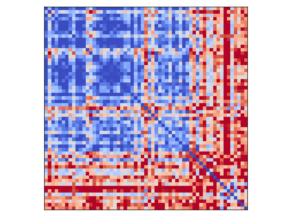
(a) LabelMe $\#$1$\sim$59

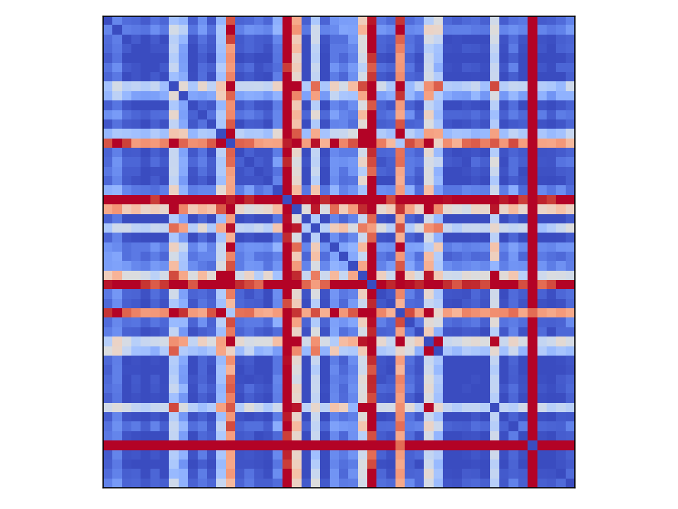
(b) CIFAR-10N $\#$50$\sim$100

Figure 3: The distances of true confusion matrices of every two annotators in LabelMe and CIFAR-10N datasets. The $\#$ denotes the index of annotators. The more blue (red) the pixel is, the smaller (larger) value it is.

Coupled Confusion Correction

Before diving into technical details, we first claim and justify an assumption that: In real-world crowd-sourcing datasets, there are various annotators who share similar expertise.

We hereby take two common real-world crowd-sourcing datasets as examples, including LabelMe and CIFAR-10N (Rodrigues and Pereira 2018; Wei et al. 2022b; Chu, Ma, and Wang 2021). We calculate the true confusion matrices of each annotators $(CM^{r})_{(C\times C)}$ in such two datasets as follows:

$$CM^{r}_{p,q}=\left\{\begin{aligned} &0,\quad\quad\quad\quad\,\,\text{if}\sum_{i=1}^{N}\mathds{1}[\mathcal{A}_{i,r}\cap y_{i}=p]=0\\ &\frac{\sum_{i=1}^{N}\mathds{1}[\mathcal{A}_{i,r}\cap y_{i}=p\cap\tilde{y}_{i}^{r}=q]}{\sum_{i=1}^{N}\mathds{1}[\mathcal{A}_{i,r}\cap y_{i}=p]},\quad\text{else}\end{aligned}\right.$$

where $y_{i}$ denotes the true label of $i$-th instance. After getting the true confusion matrices, we calculate the distance between the true confusion matrices of every two annotators using mean-square-error. Figure 3 illustrates the confusion distances between annotators in the LabelMe and CIFAR-10N datasets, where blue and red indicate small and large distances, respectively. As we can tell, there are many “blue patches” in the distance matrices, which suggests that the confusion matrices of annotators in such patch is similar to each other. Therefore, if their expertise can be considered together, the annotation sparsity can also be alleviated to some extent.

Overview of Our Approach. In this paper, to alleviate the annotation sparsity, we propose Coupled Confusion Correction (CCC), where we simultaneously train two models and utilize the meta set distilled to correct the ASCPs learned by each other. Following (Cao et al. 2019; Chu, Ma, and Wang 2021; Rodrigues and Pereira 2018; Albarqouni et al. 2016), we also adopt the confusion matrices to model the annotators’ expertise. A set of confusion-correcting-matrices $\{\bm{V}^{r}\}_{r=1}^{G}$ are regarded as meta parameters to correct the confusion matrices of annotators $\{\bm{T}^{r}\}_{r=1}^{R}$, where $G$ is a hyper parameter indicating how many similar groups of annotators are. We run the K-Means (Forgy 1965; Arthur and Vassilvitskii 2007) method on the learned confusion matrices $\{\bm{T}^{r}\}_{r=1}^{R}$ to obtain their group indexes at each epoch. Unlike CrowdLayer (Rodrigues and Pereira 2018), which only updates the confusion matrices based on individual annotations, CCC allows the confusion matrix of one annotator to be updated under the supervision of both his/her group’s annotations and the meta set. This makes CCC more resilient to annotation sparsity, leading to improved classifier performance. In the following, we first explain why the supervised information can flow back from the meta set to the confusion-correcting-matrices. Then we present the distillation strategy of the meta set and the training objectives of different stages in our CCC. The framework of our method is illustrated in Figure 2 and the pseudo code can be found in the Appendix.

Correcting Confusion Matrices by Meta Set. In our CCC, the corrected confusion matrices are obtained through the following bi-level optimization:

$$\{\bm{V}^{r\star}\}_{r=1}^{G}=\operatorname*{arg\,min}_{\{\bm{V}^{r}\}_{r=1}^{G}}\frac{1}{M}\sum_{j=1}^{M}\mathcal{L}_{j}^{meta}(\bm{\theta}^{\star}),\text{s.t.,}$$ (8)

$$\bm{\theta}^{\star},\{\bm{T}^{r\star}\}_{r=1}^{R}=\operatorname*{arg\,min}_{\bm{\theta},\{\bm{T}^{r}\}_{r=1}^{R}}\frac{1}{N}\sum_{i=1}^{N}\sum_{r=1}^{R}\mathds{1}[\mathcal{A}_{i,r}]\mathcal{L}_{i,r}^{tra}(\bm{T}_{cor}^{r},\bm{\theta})$$

where $\bm{T}_{cor}^{r}=\bm{T}^{r}+\bm{V}^{g(r)}$ denotes the corrected confusion matrix of $r$-th annotator with $g(r)$ representing the index of group which the $r$-th annotator belongs to. Let $\ell$ denotes the cross entropy loss function, the meta loss here is then defined as $\mathcal{L}_{j}^{meta}(\bm{\theta}^{\star})=\ell(f(\bm{x}^{meta}_{j}|\bm{\theta}^{\star}),y^{meta}_{j})$, and the training loss is $\mathcal{L}_{i,r}^{tra}(\bm{T}_{cor}^{r},\bm{\theta})=\ell((\bm{T}^{r}+\bm{V}^{g(r)})f(\bm{x}_{i}|\bm{\theta}),\tilde{y}_{i}^{r})$. Next, let us focus on the gradient w.r.t. the confusion-correcting-matrix of $r_{0}$-th annotator $\bm{V}^{g(r_{0})}$ (denoted by $\bm{g}^{r_{0}}_{cor}$):

Comparing Eq. (7) and Eq. (9), we can see that every data in the meta set contribute to the overall gradient of the confusion-correcting-matrix of the $r_{0}$-th annotator. In this way, the learned confusion matrices can be corrected under the supervision of the meta set. Remarkably, because we cluster annotators with similar expertise, the confusion-correcting-matrices of two annotators ($r_{0},r_{1}$) can be updated together as long as they belong to the same group $\left(g(r_{0})=g(r_{1})\right)$, which further hinders the influence of annotation sparsity.

Distilling Meta Sets using Two Models. In most previous meta learning approaches (Shu et al. 2019; Wang, Hu, and Hu 2020), the meta set is demanded to be provided in addition to the training set, which may harms the fairness of the comparison to baselines. To this end, FaMUS (Xu et al. 2021) and FSR (Zhang and Pfister 2021) provided another way to construct meta set, where it can be distilled directly from the training set. However, their methods are constrained in the single-label scenario, hence we propose a new distilling strategy to match the crowd-sourcing annotations. The algorithm is quite simple to understand, as many sample-selection-based methods pointed out (Arpit et al. 2017; Han et al. 2018; Li, Socher, and Hoi 2020), the samples with smaller loss is more likely to be clean. Therefore, for each class $c$, we first fetch all the instances that are attached with the label $c$, then we select the ones with ${M}/{C}$ smallest losses. Nevertheless, it is worth noting that in Eq. 8, if the losses of the instances that we select are already small, the supervised information that we obtain from the meta set may also be insufficient. Consequently, we simultaneously train two models to distill meta set for each other, in which way we can mitigate the confirmation bias (i.e., one model would accumulate its errors (Li, Socher, and Hoi 2020)) to ensure the meta set to be sufficiently informative while maintaining clean.

Training Objective. As stated above, in iteration $t$, we have a training mini-batch $\tilde{\mathcal{M}}=\{\bm{x}_{i},\tilde{\bm{y}}_{i}\}_{i=1}^{n}$ and a meta mini-batch $\mathcal{M}^{meta}=\{\bm{x}^{meta}_{j},{y}^{meta}_{j}\}_{j=1}^{m}$ for each model. The training objective and outcomes in three stages (virtual, meta, actual) are shown as follows:

$$\text{Virtual}: \,\frac{1}{n}\sum_{i=1}^{n}\sum_{r=1}^{R}\mathcal{L}^{tra}_{i,r}((\bm{T}^{r}_{t-1}+\bm{V}^{g(r)}_{t-1}),\bm{\theta}_{t-1})\rightarrow\hat{\bm{\theta}}_{t}$$ (10)

$$\text{Meta}: \,\frac{1}{m}\sum_{i=1}^{m}\mathcal{L}^{meta}_{j}(\hat{\bm{\theta}}_{t})\rightarrow\{\bm{V}^{r}_{t}\}_{r=1}^{G}$$ (11)

Note that the confusion-correcting-matrices are initialized as zero matrices at the beginning of each iteration, after the above two stages (i.e. the outer loop), we have obtained the corrected confusion matrices $\bm{T}_{cor}^{r}|_{t-1}=\bm{T}^{r}_{t-1}+\bm{V}^{g(r)}_{t}$, which can be used in the following actual stage (i.e. the inner loop):

$$\text{Actual}: \,\frac{1}{n}\sum_{i=1}^{n}\sum_{r=1}^{R}\mathcal{L}^{tra}_{i,r}(\bm{T}_{cor}^{r}|_{t-1},\bm{\theta}_{t-1})\rightarrow\{\bm{T}^{r}_{t}\}_{r=1}^{R},\bm{\theta}_{t}$$ (12)

Dataset		CIFAR-10				Fashion-MNIST
Method / Case		IND-I	IND-II	IND-III	IND-IV	IND-I	IND-II	IND-III	IND-IV
MajorVote	Best	55.08$\pm$0.38	47.85$\pm$2.20	54.27$\pm$1.91	66.94$\pm$1.01	84.89$\pm$2.24	79.94$\pm$2.30	76.72$\pm$1.00	89.03$\pm$0.75
	Last	41.14$\pm$0.37	32.90$\pm$0.71	42.00$\pm$0.39	60.18$\pm$1.95	61.00$\pm$0.65	51.31$\pm$0.56	56.88$\pm$0.29	78.02$\pm$0.52
CrowdLayer	Best	63.06$\pm$1.49	53.50$\pm$1.24	59.39$\pm$1.21	69.09$\pm$0.62	88.83$\pm$0.61	84.77$\pm$2.09	87.01$\pm$3.05	90.31$\pm$0.42
	Last	54.78$\pm$0.49	43.71$\pm$0.62	53.17$\pm$0.34	67.51$\pm$0.91	75.89$\pm$0.19	66.39$\pm$0.21	66.67$\pm$0.47	84.67$\pm$0.20
DoctorNet	Best	69.63$\pm$0.86	63.43$\pm$1.46	69.77$\pm$2.02	76.25$\pm$0.47	90.54$\pm$0.23	88.78$\pm$0.68	88.29$\pm$1.20	90.96$\pm$0.32
	Last	66.80$\pm$1.12	57.95$\pm$1.09	65.40$\pm$0.98	74.60$\pm$0.45	83.01$\pm$0.13	76.07$\pm$0.49	75.77$\pm$0.20	86.78$\pm$0.19
Max-MIG	Best	71.63$\pm$1.15	65.52$\pm$0.99	69.73$\pm$1.09	75.97$\pm$0.39	91.03$\pm$0.38	90.15$\pm$0.45	90.07$\pm$0.49	91.32$\pm$0.25
	Last	66.47$\pm$0.48	56.63$\pm$0.46	61.68$\pm$0.63	73.19$\pm$0.59	82.16$\pm$0.32	73.33$\pm$0.39	73.53$\pm$0.47	86.16$\pm$0.37
CoNAL	Best	67.28$\pm$1.24	59.27$\pm$1.53	65.93$\pm$0.15	78.16$\pm$0.27	89.95$\pm$0.30	87.62$\pm$0.88	89.13$\pm$0.44	91.72$\pm$0.14
	Last	56.18$\pm$0.30	47.02$\pm$0.65	57.16$\pm$0.49	71.96$\pm$0.53	75.27$\pm$0.17	65.80$\pm$0.32	71.16$\pm$0.29	86.67$\pm$0.25
UnionNet	Best	74.67$\pm$0.82	68.92$\pm$0.96	71.52$\pm$1.14	79.29$\pm$0.65	91.30$\pm$0.37	90.09$\pm$0.42	89.67$\pm$0.58	91.61$\pm$0.25
	Last	74.44$\pm$0.60	63.41$\pm$0.75	67.00$\pm$0.42	78.78$\pm$0.74	88.22$\pm$0.19	78.29$\pm$0.29	79.09$\pm$0.54	90.56$\pm$0.21
CCC (Ours)	Best	80.16$\pm$0.23	75.33$\pm$0.43	78.28$\pm$0.25	83.06$\pm$0.26	92.59$\pm$0.01	91.93$\pm$0.18	92.50$\pm$0.13	93.23$\pm$0.06
	M.I.	$\uparrow$ 5.49	$\uparrow$ 6.41	$\uparrow$ 6.76	$\uparrow$ 3.77	$\uparrow$ 1.29	$\uparrow$ 1.78	$\uparrow$ 2.43	$\uparrow$ 1.51
	Last	79.50$\pm$0.12	73.52$\pm$0.39	77.20$\pm$0.26	82.56$\pm$0.07	92.51$\pm$0.06	91.58$\pm$0.39	92.17$\pm$0.04	93.14$\pm$0.06
	M.I.	$\uparrow$ 5.06	$\uparrow$ 10.11	$\uparrow$ 10.20	$\uparrow$ 3.78	$\uparrow$ 4.29	$\uparrow$ 13.29	$\uparrow$ 13.08	$\uparrow$ 2.58
Method / Case		COR-I	COR-II	COR-III	COR-IV	COR-I	COR-II	COR-III	COR-IV
MajorVote	Best	59.18$\pm$3.38	63.26$\pm$1.39	67.03$\pm$1.00	67.39$\pm$1.63	85.73$\pm$1.51	85.22$\pm$1.99	89.38$\pm$0.38	89.25$\pm$0.70
	Last	43.57$\pm$0.61	50.36$\pm$0.76	59.04$\pm$0.62	57.97$\pm$1.07	60.83$\pm$0.57	66.11$\pm$0.83	79.69$\pm$0.77	75.68$\pm$0.46
CrowdLayer	Best	62.51$\pm$1.12	67.45$\pm$1.03	69.24$\pm$0.69	70.07$\pm$0.40	88.49$\pm$0.44	89.87$\pm$0.17	90.19$\pm$0.28	89.88$\pm$0.23
	Last	54.61$\pm$0.52	62.70$\pm$0.41	66.27$\pm$0.28	68.64$\pm$0.50	76.02$\pm$0.20	79.15$\pm$0.17	85.33$\pm$0.09	83.93$\pm$0.19
DoctorNet	Best	67.30$\pm$1.28	74.01$\pm$0.62	73.87$\pm$0.48	77.52$\pm$0.49	89.29$\pm$0.37	90.54$\pm$0.32	90.36$\pm$0.21	90.86$\pm$0.21
	Last	63.02$\pm$0.92	71.48$\pm$1.22	72.19$\pm$0.41	76.80$\pm$0.59	82.38$\pm$0.17	84.78$\pm$0.37	86.65$\pm$0.18	87.28$\pm$0.16
Max-MIG	Best	71.69$\pm$0.68	74.55$\pm$0.56	76.83$\pm$0.30	75.81$\pm$0.68	90.27$\pm$0.07	91.26$\pm$0.17	91.38$\pm$0.16	91.17$\pm$0.28
	Last	67.19$\pm$0.33	73.28$\pm$0.60	75.82$\pm$0.46	73.94$\pm$0.60	81.20$\pm$0.33	84.58$\pm$0.49	88.14$\pm$0.21	84.83$\pm$0.49
CoNAL	Best	69.33$\pm$0.46	72.21$\pm$0.30	75.97$\pm$0.19	79.82$\pm$0.49	89.48$\pm$0.34	90.79$\pm$0.40	91.37$\pm$0.10	92.02$\pm$0.14
	Last	58.24$\pm$0.63	64.10$\pm$0.27	68.42$\pm$0.65	73.82$\pm$0.83	75.49$\pm$0.30	78.36$\pm$0.28	85.93$\pm$0.40	88.47$\pm$0.47
UnionNet	Best	74.46$\pm$0.43	78.13$\pm$0.43	80.02$\pm$0.51	80.99$\pm$0.66	90.83$\pm$0.40	91.52$\pm$0.14	91.94$\pm$0.22	92.31$\pm$0.22
	Last	72.84$\pm$0.31	77.58$\pm$0.47	79.37$\pm$0.62	80.85$\pm$0.66	85.32$\pm$0.21	88.60$\pm$0.37	91.82$\pm$0.41	92.24$\pm$0.32
CCC (Ours)	Best	80.77$\pm$0.10	81.84$\pm$0.14	83.32$\pm$0.13	82.72$\pm$0.11	91.93$\pm$0.09	92.87$\pm$0.06	93.01$\pm$0.07	93.18$\pm$0.10
	M.I.	$\uparrow$ 6.31	$\uparrow$ 3.71	$\uparrow$ 3.30	$\uparrow$ 1.73	$\uparrow$ 1.10	$\uparrow$ 1.35	$\uparrow$ 1.07	$\uparrow$ 0.87
	Last	80.07$\pm$0.22	81.50$\pm$0.09	83.07$\pm$0.13	82.53$\pm$0.20	91.75$\pm$0.11	92.70$\pm$0.07	92.88$\pm$0.07	93.10$\pm$0.09
	M.I.	$\uparrow$ 7.23	$\uparrow$ 3.92	$\uparrow$ 3.70	$\uparrow$ 1.68	$\uparrow$ 6.43	$\uparrow$ 4.10	$\uparrow$ 1.06	$\uparrow$ 0.86

Table 1: Comparison with state-of-the-art approaches in test accuracy ($\%$) on synthetic datasets with independent (IND) and correlated (COR) confusions. The best results are in bold. The “M.I.” represents minimal improvement.

Experiments

We conduct experiments on two types of synthetic datasets (independent and correlated confusion) and three real-world datasets. To make the results reliable, all experiments are repeated three times with different random seeds, both the best accuracy on test set during training and the accuracy at the last epoch is reported. All experiments are conducted on a single NVIDIA RTX 3090 GPU. Due to space limitation, we only present the brief descriptions of datasets and results in the main paper, more information about datasets and the implementation details can be found in the Appendix.

Baselines. We compare our method with extensive state-of-the-art approaches. The compared approaches include: (1) Majority Vote (Whitehill et al. 2009). (2) Crowd Layer (Rodrigues and Pereira 2018). (3) Doctor Net (Guan et al. 2018). (4) Max-MIG (Cao et al. 2019). (5) CoNAL (Chu, Ma, and Wang 2021). (6) UnionNet (Wei et al. 2022a).

Evaluation on Synthetic Datasets

Datasets. We evaluate our method on a variety of synthetic datasets, which are derived from two widely used datasets, i.e., CIFAR-10 (Krizhevsky, Hinton et al. 2009) and Fashion-MNIST (Xiao, Rasul, and Vollgraf 2017). In general, we divide the synthetic datasets into two types: 1) independent confusion, where the confusions of annotators are independent from each other and 2) correlated confusion, where the confusions among different annotators may affect each other. Due to the limited page, we provide the generation details of these two confusions in the Appendix.

Results. Table 1 shows the results on synthetic datasets with independent and correlated confusions. As shown, our CCC achieves superior performance than state-of-the-art methods across all scenarios. Based on the minimal improvement (M.I.) results, it is evident that the M.I. achieved at the last epoch is notable, which suggests that our CCC effectively prevents over-fitting while improving the model’s best performance. On the other hand, the common baseline approach Majority Voting performs worst consistently, and the accuracy at last epoch decreases a lot compared to the best one, which is consistent with other works (Cao et al. 2019; Chu, Ma, and Wang 2021; Li et al. 2023a; Rodrigues and Pereira 2018; Li et al. 2020). This is because the naive majority vote fails to consider the difference among confusions of annotators, making the DNN eventually over-fits to the noisy labels. As for the approaches that consider annotators differently, their results are unstable, none of them performs better than any other methods consistently. The accuracy drop is also observed between the best and last epochs, the reason of which lies within that the ASCPs (e.g. confusion matrices in (Rodrigues and Pereira 2018; Cao et al. 2019)) of some annotators are poorly modeled, which makes the model finally memorize the noisy labels. It is worth noting that without using meta set to correct the learned confusion matrices, CCC will reduce to CrowdLayer (Rodrigues and Pereira 2018). With the use of the meta set, the results of our CCC is significantly improved compared to that of CrowdLayer (Rodrigues and Pereira 2018). This suggests that the confusion matrices employed in CCC are better able to model the expertise of annotators.

Evaluation on Real-World Datasets

Datasets. Three real-world datasets are adopted for evaluation, including LabelMe (Rodrigues and Pereira 2018), CIFAR-10N (Wei et al. 2022b) and MUSIC (Rodrigues, Pereira, and Ribeiro 2014). The first two datasets are image classification datasets, while the last one is a music genre classification dataset. The annotations of these real-world datasets are collected on Amazon Mechanical Turk.

Method / Dataset		LabelMe	CIFAR-10N	MUSIC
MajorVote	Best	80.72${\pm 0.45}$	81.08${\pm 0.34}$	67.67$\pm$0.98
	Last	77.19${\pm 1.18}$	80.89${\pm 0.25}$	62.00$\pm$1.05
CrowdLayer	Best	84.01${\pm 0.36}$	80.43${\pm 0.25}$	71.67$\pm$0.50
	Last	82.32${\pm 0.41}$	80.14${\pm 0.28}$	69.33$\pm$0.93
DoctorNet	Best	82.32${\pm 0.49}$	83.68${\pm 0.33}$	67.33$\pm$0.74
	Last	81.73${\pm 0.49}$	83.32${\pm 0.29}$	65.33$\pm$0.75
Max-MIG	Best	86.28${\pm 0.35}$	83.25${\pm 0.47}$	75.33$\pm$0.69
	Last	83.16${\pm 0.66}$	83.12${\pm 0.63}$	71.67$\pm$0.93
CoNAL	Best	87.46${\pm 0.53}$	82.51${\pm 0.15}$	74.00$\pm$0.89
	Last	84.85${\pm}$0.91	80.92${\pm 0.28}$	68.67$\pm$1.88
UnionNet	Best	85.19${\pm 0.42}$	82.66${\pm 1.12}$	72.33$\pm$0.58
	Last	82.66${\pm 0.38}$	82.32${\pm 1.09}$	68.33$\pm$0.91
CCC (Ours)	Best	87.65$\pm$1.10	86.36$\pm$0.05	76.22$\pm$0.42
	M.I.	$\uparrow$ 0.19	$\uparrow$ 2.68	$\uparrow$ 0.89
	Last	84.79$\pm$0.80	86.12$\pm$0.12	72.89$\pm$0.68
	M.I.	$\downarrow$ 0.06	$\uparrow$ 2.80	$\uparrow$ 1.22

Table 2: Comparison with state-of-the-art approaches in test accuracy ($\%$) on real-world datasets. The best results are in bold. The “M.I.” represents minimal improvement.

Results. The evaluation results on three real-world datasets are presented in Table 2. As shown, our CCC outperforms other methods in two metrics (best and last) on CIFAR-10N and MUSIC. Additionally, on the LabelMe dataset, our CCC yields a new state-of-the-art result in terms of the best accuracy during training and achieves competitive accuracy results at the last epoch. These results provide evidence that our CCC is effective in handling real-world crowd-sourced annotations. Remarkably, the results of our CCC on CIFAR-10N are even comparable to the results that were trained with clean labels (refer to the Appendix). This means that the expertise of annotators in the CIFAR-10N dataset has been fully captured by our CCC.

Ablation Study

Annotation Sparsity. To study the performance of CCC under different sparsity levels, we conduct experiments under different average numbers of annotations. To this end, we synthesize 4 more sets of annotations for the CIFAR-10 (Krizhevsky, Hinton et al. 2009) benchmark with an average number of annotations of 1,5,7,9, the confusion patterns of these datasets are identical to CIFAR-10-IND-I. The first chart in Figure 4 depicts the corresponding results compared to CrowdLayer (Rodrigues and Pereira 2018), from which we can see that our CCC yields higher test accuracy in both best and last metrics. Remarkably, even in the sparsest case, our CCC can still bring significant improvement (17.15$\%$ on best and 32.95$\%$ on last).

Number of Annotator Groups. As shown in Figure 3, there are various annotator groups in crowd-sourcing datasets, hence it is not necessary to consider all the annotators separately. However, the number of annotator groups is hard to identify, because the true labels are not available in practice. Therefore, in our CCC, the number of annotator groups $G$ is deemed as a hyper-parameter. We conduct the ablation study of $G$ on the CIFAR-10-IND-I dataset. The second chart in Figure 4 demonstrates the test accuracy ($\%$) over different $G$’s. If $G$ is small, distinct annotators may be grouped together, leading to potential interference between their annotations. Conversely, if $G$ is large, similar annotators may be considered separately, resulting in poor modeling of their expertise due to annotation sparsity.

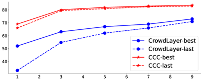
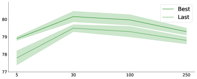
Figure 4: The ablation studies on sparsity level (top) and number of annotator groups (bottom). The horizontal axis represents average number of annotators (top) and number of annotator groups (bottom), while the vertical axis denotes test accuracy.

Conclusions

In this work, we proposed a novel framework called Coupled Confusion Correction (CCC) to learn from multiple annotators, where the confusion matrices learned by one model can be corrected by the meta set distilled from the other. To further alleviate annotation sparsity, we unite various annotators based on their expertise using K-Means so that their confusion matrices could be corrected together. Besides, we reveal a common but neglected phenomenon in crowd-sourcing datasets that there are always annotators who provide seldom labels, which hinders the modeling of their expertise. Through extensive experiments across both synthetic and real-world datasets, we show that our CCC significantly outperforms other state-of-the-art approaches.

Appendix A Related Works

The problem we focused on in this paper is learning from crowds, and the learning paradigm we used is meta learning. Therefore, we hereby briefly review the related works from these two disciplines:

Learning from Crowds (LFC). In the crowd-sourcing setting, one instance is associated with multiple labels, some of which could be noisy. To mitigate the influence of label noise, one common direction is to aggregate such noisy labels into a more reliable one and train the downstream tasks with these aggregated labels. For example, the Majority Voting (Whitehill et al. 2009; Han et al. 2019a; Schwenker 2013) is one of the most simplest and widely-used methods in aggregating crowd-sourcing labels. It naively assumes that all the annotators are equally reliable (i.e. have the same expertise), which is criticized for not able to handle the scenario where most annotators have relatively low expertise (Li et al. 2014; Tian, Zhu, and Qiaoben 2019; Karger, Oh, and Shah 2011; Dalvi et al. 2013). Further, some more advanced aggregated methods are proposed, where the expertise of annotators are deemed to be different, including the Weighted Majority Voting (Li et al. 2014), max-margin majority voting (Tian, Zhu, and Qiaoben 2019), tensor factorization approaches (Karger, Oh, and Shah 2011; Dalvi et al. 2013). Although Majority Voting and its variants provide a way to alleviate label noises, it is not always feasible to aggregate the labels, and these pipeline of methods may suffer from error propagation (Whitehill et al. 2009; Han et al. 2019a; Schwenker 2013).

On the other hand, by viewing the true label as an un-observable latent variable, many approaches tend to infer the true labels based on the Expectation–Maximization (EM) algorithm (Dawid and Skene 1979). Among them, the Dawid and Skene’s model (Dawid and Skene 1979) serves as the basis of many works for aggregating labels from different annotators with different levels of expertise. For example, the approach proposed in (Whitehill et al. 2009) extends Dawid and Skene’s model by jointly accounting for item difficulty. Similarly, (Ipeirotis, Provost, and Wang 2010) proposed to extract a confident score using Dawid and Skene’s model, where the extracted score can be further used to prune low-quality annotators.

Despite the effectiveness of these EM-based algorithms, the training process often suffers from its computational complexity. This issue can be more severe when DNNs are adopted as the classifier, for the DNNs usually have massive parameters. To this end, many approaches are designed to directly model the annotator-specific expertise so as to use all the annotations on the fly (Albarqouni et al. 2016; Chu, Ma, and Wang 2021; Cao et al. 2019; Li et al. 2023a; Rodrigues and Pereira 2018). For instance, the CrowdLayer (Rodrigues and Pereira 2018) is proposed to train a DNN directly with crowd-sourcing labels. Multiple “crowd layers” (linear layers without biases, also called confusion matrices) are added to the last softmax layer of the backbone DNN to capture the annotator-specific expertise of each annotator (Rodrigues and Pereira 2018), in which way the backbone DNN and the “crowd layers” can be optimized simultaneously during training. Following this line of work, CoNAL (Chu, Ma, and Wang 2021) proposed an approach to model a common confusion matrix except for the individual ones. CoNAL assumes that the annotation noise is attributed to two sources (common noise and individual noise), and combines these two noise by a Bernoulli random variable. Moreover, UnionNet (Wei et al. 2022a) unites all the noisy labels into a single “united label” in an one-hot manner and model the confusions by a single confusion matrix. In addition, there are some methods that do not rely on the confusion matrices but model the expertise of each annotator respectively as the CrowdLayer and CoNAL do. For example, the DoctorNet (Guan et al. 2018) aims to train a DNN with multiple softmax outputs to exploit all the annotations. Compared with the aforementioned aggregated methods like Majority Voting and its variants, the algorithms that learn the ASCPs (confusion matrices or multiple softmax outputs) simultaneously have achieved equal or even more promising performance. However, one of the major limitations of these methods is that learning such ASCPs usually suffers from the annotation sparsity, which is elaborated in Section 2.2.

Dataset			Split			N.R.1	N.R.2	$\#$Annotators		Experiment Configuration
			$\#$Train	$\#$Test	$\#$Valid	$(\%)$	$(\%)$	Total	Mean	Arch.	B.S.	Optim.	I.L.R.	$\#$Epochs		$M$	$G$
- CIFAR -	10N		45K	10K	5K	02.13	17.71	747	3	ResNet-34	128	SGD	10-2	60	10	1K	50
	IND	I				19.61	56.88	250									30
		II				26.87	63.44
		III				20.75	56.75
		IV				09.68	46.21
	COR	I				17.02	54.12
		II				14.18	50.70
		III				09.08	44.99
		IV				10.07	46.72
- Fashion-MNIST -	IND	I	54K	10K	6K	18.73	55.82			ResNet-18
		II				26.14	62.62
		III				21.45	57.98
		IV				09.66	45.97
	COR	I				19.39	56.64
		II				15.77	51.74
		III				09.27	45.03
		IV				10.67	47.66
LabelMe			10K	1188	500	11.10	25.95	59	2.5	VGG-16		Adam	10-4	200	50		25
MUSIC			700	300	0	12.71	43.97	44	4.2	FC			10-2			160	20

Table 3: The summary of datasets information and experiment configurations. The first and second columns of $\#$Epochs is the total epochs for training and warm-up epochs respectively. Abbreviations: Arch.: the architecture of the backbone network; B.S.: batch size; Optim.: the type of optimizer; I.L.R.: initial learning rate; $M$: the size of meta set; $G$: the number of annotator groups.

Meta Learning. Inspired by the developments of meta-learning(Jones 2001; Maclaurin, Duvenaud, and Adams 2015; Zoph and Le 2017), many approaches are proposed to train a DNN that are robust to label noise (Shu et al. 2019; Wang, Hu, and Hu 2020; Zheng, Awadallah, and Dumais 2021; Xu et al. 2021). For instance, MLC (Wang, Hu, and Hu 2020) designed a loss correction method where the transition matrix is learned via meta-learning. And the transition matrix is further used to correct the loss during training, making the empirical risk over noisy dataset to be consistent with the risk over clean dataset. (Zheng, Awadallah, and Dumais 2021) use meta-learning to train a label-correction model during training, where the true labels can be inferred given instance features and noisy labels. In addition, meta-learning is also applied to learn an adaptive weighting scheme in (Shu et al. 2019), through which the weight of instances are adjusted. However, the great capability of meta learning has not been exploit in crowd-sourcing setting yet, which also motivates us to explore its performance in LFC.

Appendix B Pseudo Code of CCC

The pseudo code of CCC is presented in Algorithm 1

Algorithm 1 Coupled Confusion Correction (CCC)

Input: main parameters $\bm{\theta}_{1},\bm{\theta}_{2},\{\bm{T}^{r}_{1},\bm{T}^{r}_{2}\}_{r=1}^{R}$, meta parameters $\{\bm{V}^{r}_{1},\bm{V}^{r}_{2}\}_{r=1}^{G}$, training set $\tilde{\mathcal{D}}$, max epochs $E$, warmup epochs $E_{w}$

1:  for $e=0,...,E-1$ do

2:     if $e<E_{w}$ then

3:        $\bm{\theta}_{1},\bm{\theta}_{2}=$ Warmup $(\tilde{\mathcal{D}},\bm{\theta}_{1},\bm{\theta}_{2})$ //warmup the model using CrowdLayer to prepare for the distillation stage

4:     else if $e<E$ then

5:        $\mathcal{D}^{meta}_{1}\stackrel{{\scriptstyle\text{distill}}}{{\underset{\bm{\theta}_{2}}{\longleftarrow}}}\tilde{\mathcal{D}},\quad\mathcal{D}^{meta}_{2}\stackrel{{\scriptstyle\text{distill}}}{{\underset{\bm{\theta}_{1}}{\longleftarrow}}}\tilde{\mathcal{D}}$ //coupled distillation

6:        Initialize $\{\bm{V}^{r}_{1},\bm{V}^{r}_{2}\}_{r=1}^{G}$ as zero tensors

7:        Get the group index of each annotator using K-Means $g(r)=\text{K-Means}(\{\bm{T}^{r}_{1},\bm{T}^{r}_{2}\}_{r=1}^{R})$

8:        for $k=1,2$ do

9:           for $i=1$ to num$\_$iters do

10:              Fetch training-batch $\tilde{\mathcal{M}}\leftarrow\tilde{\mathcal{D}}$

11:              Fetch meta-batch $\mathcal{M}^{meta}_{k}\leftarrow\mathcal{D}^{meta}_{k}$

12:              Update $\{\bm{V}^{r}_{k}\}_{r=1}^{G}$ according to Eq. (10) and Eq. (11)//outer loop of the bi-level optimization

13:              Update $\bm{\theta}_{k},\{\bm{T}^{r}_{k}\}_{r=1}^{R}$ according to Eq. (12)//inner loop of the bi-level optimization

14:           end for

15:        end for

16:     end if

17:  end for

18:  return $\bm{\theta}_{1},\bm{\theta}_{2}$

Confusion Type	Independent Confusion				Correlated Confusion
Set Index	IND-I	IND-II	IND-III	IND-IV	COR-I	COR-II	COR-III	COR-IV
Pattern-I	sym.	sym.	pair	sym.	sym.	pair	pair	sym.
	0.3	0.4	0.3	0.3	0.4	0.5	0.4	0.5
Pattern-II	sym.	class	pair	sym.	class	class	sym.	pair
	0.5	2,5,9	0.6	0.5	2,5,9	0,6,8	0.5	0.7
Pattern-III	pair	pair	class	sym.	dummy	supp.	oppo.	pair
	0.6	0.6	0,4,5	0.7				0.3
Pattern-IV	class	class	class	pair	supp.	oppo.	supp.	oppo.
	1,3,4,6,8	0,6,8	1,3,4,6,8	0.5
Pattern-V	dummy	dummy	dummy	pair	oppo.	copy	copy	supp.
				0.3

Table 4: The confusion patterns of the synthetic datasets. sym.: symmetrical confusion; class: class-wise confusion; supp.: supportive confusion; oppo.: opposite confusion.

Appendix C More Experiment Details

Generation of Two confusions

For independent confusion, we consider four types of confusion patterns to generate the crowd-sourcing annotations, including 1) symmetrical-$\epsilon$: the annotator would provide true labels with probability $1-\epsilon$ and provide wrong labels uniformly with probability $\frac{\epsilon}{C-1}$, 2) pair-$\epsilon$: the annotator may confuse with similar class-pairs, it would label correctly with probability $1-\epsilon$ and provide the label from another class with probability $\epsilon$, 3) class-wise-$c_{0},c_{1},...c_{w}$: the annotator would label the instances from classes $c_{0},c_{1},...c_{w}$ correctly with probability $1$, but it will choose labels uniformly for instances from other classes, 4) dummy: the annotator would choose labels uniformly with probability $\frac{1}{C}$ for all classes. Note that the dummy type confusion simulates the case where some annotators pick labels randomly to get rewards on the crowd-sourcing platforms, which is also taken into consideration in (Wei et al. 2022b). For correlated confusion, following (Li et al. 2023a), three types of correlated patterns are included: 1) copy, where the annotator randomly picks another annotator and copies its label, 2) supportive, where the annotator gives the right answer if another randomly picked annotator’s answer is right, and give uniformly distributed answers otherwise, 3) opposite, which is on the contrary of supportive pattern, the annotator gives the right answer if another randomly picked annotator’s answer is wrong, and give uniformly distributed answers otherwise.

As stated before, in real-world crowd-sourcing datasets, there are always some annotators who only provide seldom labels (as shown in Figure 1). However, previous works failed to take that issue into consideration when synthesizing crowd-sourcing annotations, which is actually an ubiquitous and harmful one as we analysed in Section 2.2. Therefore, we propose to use Beta distribution when generating the crowd-sourcing annotations, the overall process can be summarized as follows:

$\bullet$ For each annotator, generate its annotations based on the true labels and its confusion pattern (pre-defined).

$\bullet$ For each instance, select $k$ annotators and prune the annotations of others, the probabilities of selecting each annotator is set to follow a Beta density function $P\sim Beta(\alpha,\beta)$.

In this way, the synthetic datasets will be more consistent with real-world ones. The parameters of Beta distribution is fixed as $\alpha=1.5,\beta=3$ and $k$ is set to 3 in all synthetic datasets. To cover more scenarios, for each type of confusion, we generate $4$ sets of synthetic annotations with independent/correlated confusion for each benchmark dataset. Each set has $5$ different confusion patterns, and $50$ annotators are generated according to each confusion pattern, with a total of $250$ annotators. Note that the confusion patterns are shared between the two benchmark datasets. The confusion patterns of both independent and correlated types are shown in Table 4 in the Appendix.

Datasets Descriptions

Synthetic Datasets. CIFAR-10 dataset (Krizhevsky, Hinton et al. 2009) has $50K$ training images and $10K$ test images with shape $32\times 32\times 3$, each image is associated with a label from $10$ classes. Fashion-MNIST (Xiao, Rasul, and Vollgraf 2017) has $60K$ training images and $10K$ test images with shape $28\times 28$, same as CIFAR-10, each image is associated with a label from $10$ classes. In our experiments on synthetic datasets, $10\%$ of the training set is retained as a validation set, and the rest training labels are manually flipped to noisy crowd-sourcing labels. The detailed confusion patterns of each confusion types are listed in Table 4.

Real-World Datasets. We use three real-world crowd-sourcing datasets in this paper, including LabelMe (Rodrigues and Pereira 2018), CIFAR-10N (Wei et al. 2022b) and MUSIC (Rodrigues, Pereira, and Ribeiro 2014). The labels of the three real-world datasets were all collected from Amazon Mechanical Turk by human. LabelMe is an $8$-class image classification dataset containing $2688$ images in total, including $1K$ training images, $1188$ test images and $500$ validation images. Its training images are labeled by 59 annotators in total, with an average of $2.5$ annotators per image. Following the image pre-processing approach in (Rodrigues and Pereira 2018; Cao et al. 2019; Chu, Ma, and Wang 2021), the $1K$ training images are augmented to $10K$ images. CIFAR-10N (Wei et al. 2022b) dataset consists of the original CIFAR-10 training images with re-collected labels. Each image in CIFAR-10N is labeled by $3$ annotators, with a total of $747$ annotators. MUSIC is a music genre classification dataset, which consist of $1K$ music pieces with 30 seconds length. The $1K$ music pieces are divided into a training set of $700$ pieces and a test set of $300$ pieces. All the music pieces are from 10 music genres and are labeled by 44 annotators in total, with an average of 4.2 annotators per piece.

The information of all the datasets we use is summarized in Table 3, where the noise rate (N.R.) is calculated as:

$$N.R._{1}=\frac{\sum_{i=1}^{N}\mathds{1}[y_{i}\notin\tilde{\bm{y}_{i}}]}{N},$$

$$N.R._{2}=\frac{\sum_{i=1}^{N}\sum_{j=1}^{R}\mathds{1}[\mathcal{A}_{i,j}=1]*\mathds{1}[\tilde{y}_{i}^{r}\neq y_{i}]}{\sum_{i=1}^{N}\sum_{j=1}^{R}\mathds{1}[\mathcal{A}_{i,j}=1]}.$$

The $N.R._{1}$ metric represents the overall noise level of the dataset. Specifically, an instance’s crowd-sourcing label $\tilde{\bm{y}}$ are not considered noisy as long as at least one annotator provides the correct label. In contrast, the $N.R._{2}$ metric represents the noise level of all the annotators: If an annotator provides a wrong label, its individual label $\tilde{y}$ will be considered noisy.

Implementation Details

All of our experiments are conducted on NVIDIA RTX3090 GPUs with Pytorch framework (Paszke et al. 2019). To ensure a fair comparison, we did not use any data augmentation techniques for all datasets except for the LabelMe dataset, as mentioned above. For all the experiments, the learning rate of virtual and actual stage are kept identical ($\eta_{v}=\eta_{a}$), while the learning rate of meta stage $\eta_{m}$ is set automatically as following:

$$\eta_{m}=\gamma\cdot\frac{Max(\{\bm{T}^{r}\}_{r=1}^{R})}{Max(\{|\bm{g}^{r}_{cor}|\}_{r=1}^{R})},$$

where $\bm{T}^{r}$ refers to the confusion matrix of the $r$-th annotator, and $\bm{g}^{r}_{cor}$ refers to the gradient of its confusion-correcting matrix. $\gamma$ is termed as “correction rate”, reflecting the extent to which the confusion matrices are corrected. Note that the “learning rate” will refer to both virtual and actual learning rates in the following. For the CIFAR-10 and Fashion-MNIST datasets, we adopt a batch size of 128, an SGD optimizer with a momentum of 0.9, weight decay of 5e-4, and an initial learning rate of 0.01. The learning rate is divided by 10 after the 40-th epoch, 60 epochs are set in total, 10 of which are used for warming up. The ResNet-34 is used for CIFAR-10 and ResNet-18 is used for Fashion-MNIST. The number of annotator groups $G$ is set to 30. For the LabelMe dataset, we adopt a batch size of 128, an Adam optimizer with a learning rate of 1e-4. 200 epochs are set in total, including 50 epochs for warming up and 150 for CCC. The number of annotator groups are set to be 25. Following (Rodrigues and Pereira 2018; Li et al. 2023a; Wei et al. 2022a), we use a pre-trained VGG-16 network followed by a fullly-conneted (FC) layer with 128 units, ReLU activations and a softmax output layer. For MUSIC, the same FC layer and output layer as LabelMe is adopted, and batch normalization is performed. we use an Adam optimizer with a learning rate of 1e-2. The batch size is set to 128. Similar to LabelMe, 200 total epochs and 50 warming up epochs are set, but the number of annotator groups for MUSIC is set to 20. The correction rate $\gamma$ is set to 0.3 for MUSIC and 0.5 for the other datasets. Additionally, the size of the meta set $M$ is set to 160 for MUSIC and 1000 for the other datasets. It is worth noting that as evidenced by previous studies (Xu et al. 2021; Zhang and Pfister 2021), the bi-level optimization is time-consuming due to the computation of hessian matrix, which makes the training inefficient. Following (Zhang and Pfister 2021), to accelerate the training process when computing the gradient of the meta loss for the CIFAR-10 and Fashion-MNIST, we only activate the linear layer of the network and detach the other layers. All of the information of datasets, experiment configurations, and hyper-parameters are summarized in Table 3.

Details of Baselines

Many baseline approaches include the initialization of confusion matrices, for the Max-MIG (Cao et al. 2019) and UnionNet (Wei et al. 2022a), following their original paper, we adopt the initialization strategy as:

$$\bm{T}^{r}(p,q)=log\frac{\sum_{i=1}^{N}Q(y_{i}=p)\mathds{1}[\tilde{y}_{i}^{r}=q]}{\sum_{i=1}^{N}Q(y_{i}=p)},$$

in which the $Q(y_{i}=p)$ is obtained by averaging all crowd-sourcing labels:

$$Q(y_{i}=p)=\frac{1}{R}\sum_{r=1}^{R}\mathds{1}[\tilde{y}_{i}^{r}=p].$$

Moreover, the original paper of UnionNet (Wei et al. 2022a) proposed two variants of UnionNet, but we only take the UnionNet-B as baseline because the UnionNet-B performs better according to the results of its original paper (Wei et al. 2022a). For CrowdLayer, following the settings in Max-MIG (Cao et al. 2019) and its original paper (Rodrigues and Pereira 2018), we initialize the confusion matrices as identity ones.

Dataset	CIFAR-10	F-MNIST	LabelMe	MUSIC
Best	86.19${\pm 0.28}$	93.80${\pm 0.15}$	91.84${\pm 0.10}$	82.00$\pm$1.14
Last	86.15${\pm 0.30}$	93.61${\pm 0.14}$	91.16${\pm 0.25}$	79.67$\pm$1.33

Table 5: Results that trained with clean (ground-truth) labels of all datasets we used. The “F-MNIST” represents the Fashion-MNIST dataset.

Appendix D Results Trained with Clean Labels

The test accuracy ($\%$) trained on clean labels of all datasets we used in this paper is reported in Table 5.

References

- Albarqouni et al. (2016) Albarqouni, S.; Baur, C.; Achilles, F.; Belagiannis, V.; Demirci, S.; and Navab, N. 2016. AggNet: Deep Learning From Crowds for Mitosis Detection in Breast Cancer Histology Images. IEEE TMI, 35(5): 1313–1321.
- Arpit et al. (2017) Arpit, D.; Jastrzebski, S.; Ballas, N.; et al. 2017. A Closer Look at Memorization in Deep Networks. In ICML, 233–242.
- Arthur and Vassilvitskii (2007) Arthur, D.; and Vassilvitskii, S. 2007. K-means++ the advantages of careful seeding. In ACM-SIAM SODA, 1027–1035.
- Biel and Gatica-Perez (2013) Biel, J.; and Gatica-Perez, D. 2013. The YouTube Lens: Crowdsourced Personality Impressions and Audiovisual Analysis of Vlogs. IEEE TMM, 15(1): 41–55.
- Buecheler et al. (2010) Buecheler, T.; Sieg, J. H.; Füchslin, R. M.; and Pfeifer, R. 2010. Crowdsourcing, Open Innovation and Collective Intelligence in the Scientific Method - A Research Agenda and Operational Framework. In ALIFE, 679–686.
- Cao et al. (2019) Cao, P.; Xu, Y.; Kong, Y.; and Wang, Y. 2019. Max-MIG: an Information Theoretic Approach for Joint Learning from Crowds. In ICLR.
- Chu, Ma, and Wang (2021) Chu, Z.; Ma, J.; and Wang, H. 2021. Learning from Crowds by Modeling Common Confusions. In AAAI, 5832–5840.
- Dalvi et al. (2013) Dalvi, N. N.; Dasgupta, A.; Kumar, R.; and Rastogi, V. 2013. Aggregating crowdsourced binary ratings. In WWW, 285–294.
- Dawid and Skene (1979) Dawid, A. P.; and Skene, A. M. 1979. Maximum likelihood estimation of observer error-rates using the EM algorithm. JRSS-C, 28(1): 20–28.
- Forgy (1965) Forgy, E. W. 1965. Cluster analysis of multivariate data: Efficiency vs. interpretability of classifications. Biometrics, 21: 768–769.
- Guan et al. (2018) Guan, M. Y.; Gulshan, V.; Dai, A. M.; and Hinton, G. E. 2018. Who Said What: Modeling Individual Labelers Improves Classification. In AAAI, 3109–3118.
- Han et al. (2019a) Han, B.; Tsang, I. W.; Chen, L.; Zhou, J. T.; and Yu, C. P. 2019a. Beyond Majority Voting: A Coarse-to-Fine Label Filtration for Heavily Noisy Labels. IEEE TNNLS, 30(12): 3774–3787.
- Han et al. (2019b) Han, B.; Yao, Q.; Pan, Y.; Tsang, I. W.; Xiao, X.; Yang, Q.; and Sugiyama, M. 2019b. Millionaire: a hint-guided approach for crowdsourcing. MLJ, 108(5): 831–858.
- Han et al. (2018) Han, B.; Yao, Q.; Yu, X.; Niu, G.; Xu, M.; Hu, W.; Tsang, I. W.; and Sugiyama, M. 2018. Co-teaching: Robust training of deep neural networks with extremely noisy labels. In NeurIPS, 8536–8546.
- Ibrahim, Nguyen, and Fu (2023) Ibrahim, S.; Nguyen, T.; and Fu, X. 2023. Deep Learning From Crowdsourced Labels: Coupled Cross-Entropy Minimization, Identifiability, and Regularization. In ICLR.
- Ipeirotis, Provost, and Wang (2010) Ipeirotis, P. G.; Provost, F. J.; and Wang, J. 2010. Quality management on Amazon Mechanical Turk. In ACM SIGKDD, 64–67.
- Ishida et al. (2020) Ishida, T.; Yamane, I.; Sakai, T.; Niu, G.; and Sugiyama, M. 2020. Do We Need Zero Training Loss After Achieving Zero Training Error? In ICML, 4604–4614.
- Jang, Gu, and Poole (2017) Jang, E.; Gu, S.; and Poole, B. 2017. Categorical Reparameterization with Gumbel-Softmax. In ICLR.
- Jones (2001) Jones, D. R. 2001. A Taxonomy of Global Optimization Methods Based on Response Surfaces. J. Glob. Optim., 21(4): 345–383.
- Karger, Oh, and Shah (2011) Karger, D. R.; Oh, S.; and Shah, D. 2011. Budget-optimal crowdsourcing using low-rank matrix approximations. In ACCCC, 284–291.
- Krizhevsky, Hinton et al. (2009) Krizhevsky, A.; Hinton, G.; et al. 2009. Learning multiple layers of features from tiny images.
- Li, Socher, and Hoi (2020) Li, J.; Socher, R.; and Hoi, S. C. H. 2020. DivideMix: Learning with Noisy Labels as Semi-supervised Learning. In ICLR.
- Li et al. (2014) Li, Q.; Li, Y.; Gao, J.; Zhao, B.; Fan, W.; and Han, J. 2014. Resolving conflicts in heterogeneous data by truth discovery and source reliability estimation. In ACM SIGMOD, 1187–1198.
- Li et al. (2020) Li, S.; Ge, S.; Hua, Y.; Zhang, C.; Wen, H.; Liu, T.; and Wang, W. 2020. Coupled-View Deep Classifier Learning from Multiple Noisy Annotators. In AAAI, 4667–4674.
- Li et al. (2023a) Li, S.; Liu, T.; Tan, J.; Zeng, D.; and Ge, S. 2023a. Trustable Co-Label Learning From Multiple Noisy Annotators. IEEE TMM, 25: 1045–1057.
- Li et al. (2023b) Li, S.; Xia, X.; Deng, J.; Ge, S.; and Liu, T. 2023b. Transferring Annotator-and Instance-dependent Transition Matrix for Learning from Crowds. arXiv.
- Lin et al. (2014) Lin, T.-Y.; Maire, M.; Belongie, S.; Hays, J.; Perona, P.; Ramanan, D.; Dollár, P.; and Zitnick, C. L. 2014. Microsoft COCO: Common Objects in Context. In ECCV, 740–755.
- Maclaurin, Duvenaud, and Adams (2015) Maclaurin, D.; Duvenaud, D.; and Adams, R. P. 2015. Gradient-based Hyperparameter Optimization through Reversible Learning. In ICML, 2113–2122.
- Paszke et al. (2019) Paszke, A.; Gross, S.; Massa, F.; et al. 2019. Pytorch: An imperative style, high-performance deep learning library. In NeurIPS, 8024–8035.
- Peterson et al. (2019) Peterson, J. C.; Battleday, R. M.; Griffiths, T. L.; and Russakovsky, O. 2019. Human Uncertainty Makes Classification More Robust. In ICCV, 9616–9625.
- Rodrigues and Pereira (2018) Rodrigues, F.; and Pereira, F. C. 2018. Deep Learning from Crowds. In AAAI, 1611–1618.
- Rodrigues, Pereira, and Ribeiro (2014) Rodrigues, F.; Pereira, F. C.; and Ribeiro, B. 2014. Gaussian Process Classification and Active Learning with Multiple Annotators. In ICML, 433–441.
- Schwenker (2013) Schwenker, F. 2013. Ensemble Methods: Foundations and Algorithms [Book Review]. IEEE CIM, 8(1): 77–79.
- Servajean et al. (2017) Servajean, M.; Joly, A.; Shasha, D. E.; Champ, J.; and Pacitti, E. 2017. Crowdsourcing Thousands of Specialized Labels: A Bayesian Active Training Approach. IEEE TMM, 19(6): 1376–1391.
- Sheng, Provost, and Ipeirotis (2008) Sheng, V. S.; Provost, F. J.; and Ipeirotis, P. G. 2008. Get another label? improving data quality and data mining using multiple, noisy labelers. In ACM SIGKDD, 614–622.
- Shu et al. (2019) Shu, J.; Xie, Q.; Yi, L.; Zhao, Q.; Zhou, S.; Xu, Z.; and Meng, D. 2019. Meta-Weight-Net: Learning an Explicit Mapping For Sample Weighting. In NeurIPS, 1917–1928.
- Simonyan and Zisserman (2015) Simonyan, K.; and Zisserman, A. 2015. Very Deep Convolutional Networks for Large-Scale Image Recognition. In ICLR.
- Snow et al. (2008) Snow, R.; O’connor, B.; Jurafsky, D.; and Ng, A. Y. 2008. Cheap and fast–but is it good? evaluating non-expert annotations for natural language tasks. In EMNLP, 254–263.
- Song et al. (2023) Song, H.; Kim, M.; Park, D.; Shin, Y.; and Lee, J.-G. 2023. Learning From Noisy Labels With Deep Neural Networks: A Survey. IEEE Transactions on Neural Networks and Learning Systems, 34(11): 8135–8153.
- Sun et al. (2018) Sun, Z.; Zhang, Q.; Li, Y.; and Tan, Y. 2018. DPPDL: A Dynamic Partial-Parallel Data Layout for Green Video Surveillance Storage. IEEE TCSVT, 28(1): 193–205.
- Tian, Zhu, and Qiaoben (2019) Tian, T.; Zhu, J.; and Qiaoben, Y. 2019. Max-Margin Majority Voting for Learning from Crowds. IEEE TPAMI, 41(10): 2480–2494.
- Wang et al. (2020) Wang, G.; Liu, X.; Li, C.; Xu, Z.; Ruan, J.; Zhu, H.; Meng, T.; Li, K.; Huang, N.; and Zhang, S. 2020. A Noise-Robust Framework for Automatic Segmentation of COVID-19 Pneumonia Lesions From CT Images. IEEE TMI, 39(8): 2653–2663.
- Wang, Hu, and Hu (2020) Wang, Z.; Hu, G.; and Hu, Q. 2020. Training Noise-Robust Deep Neural Networks via Meta-Learning. In CVPR, 4523–4532.
- Wazny (2017) Wazny, K. 2017. “Crowdsourcing” ten years in: A review. Journal of Global Health, 7(2).
- Wei et al. (2022a) Wei, H.; Xie, R.; Feng, L.; Han, B.; and An, B. 2022a. Deep Learning From Multiple Noisy Annotators as A Union. IEEE TNNLS, 1–11.
- Wei et al. (2022b) Wei, J.; Zhu, Z.; Cheng, H.; Liu, T.; Niu, G.; and Liu, Y. 2022b. Learning with Noisy Labels Revisited: A Study Using Real-World Human Annotations. In ICLR.
- Whitehill et al. (2009) Whitehill, J.; Ruvolo, P.; Wu, T.; Bergsma, J.; and Movellan, J. R. 2009. Whose Vote Should Count More: Optimal Integration of Labels from Labelers of Unknown Expertise. In NeurIPS, 2035–2043.
- Xiao, Rasul, and Vollgraf (2017) Xiao, H.; Rasul, K.; and Vollgraf, R. 2017. Fashion-mnist: a novel image dataset for benchmarking machine learning algorithms. arXiv.
- Xu et al. (2021) Xu, Y.; Zhu, L.; Jiang, L.; and Yang, Y. 2021. Faster Meta Update Strategy for Noise-Robust Deep Learning. In CVPR, 144–153.
- Yu, Deng, and Dahl (2010) Yu, D.; Deng, L.; and Dahl, G. 2010. Roles of pre-training and fine-tuning in context-dependent DBN-HMMs for real-world speech recognition. In NeurIPS. sn.
- Zhang et al. (2021) Zhang, C.; Bengio, S.; Hardt, M.; Recht, B.; and Vinyals, O. 2021. Understanding deep learning (still) requires rethinking generalization. Commun. ACM, 64(3): 107–115.
- Zhang et al. (2024) Zhang, H.; Li, S.; Wang, P.; Zeng, D.; and Ge, S. 2024. M3D: Dataset Condensation by Minimizing Maximum Mean Discrepancy. AAAI.
- Zhang (2022) Zhang, J. 2022. Knowledge learning with crowdsourcing: a brief review and systematic perspective. IEEE/CAA JAS, 9(5): 749–762.
- Zhang and Pfister (2021) Zhang, Z.; and Pfister, T. 2021. Learning Fast Sample Re-weighting Without Reward Data. In ICCV, 705–714.
- Zheng, Awadallah, and Dumais (2021) Zheng, G.; Awadallah, A. H.; and Dumais, S. T. 2021. Meta Label Correction for Noisy Label Learning. In AAAI, 11053–11061.
- Zheng et al. (2017) Zheng, Y.; Li, G.; Li, Y.; Shan, C.; and Cheng, R. 2017. Truth inference in crowdsourcing: Is the problem solved? Proceedings of the VLDB Endowment, 10(5): 541–552.
- Zoph and Le (2017) Zoph, B.; and Le, Q. V. 2017. Neural Architecture Search with Reinforcement Learning. In ICLR.