Noised Autoencoders for Point Annotation Restoration in Object Counting

Abstract

Object counting is a field of growing importance in domains such as security surveillance, urban planning, and biology. The annotation is usually provided in terms of 2D points. However, the complexity of object shapes and subjective of annotators may lead to annotation inconsistency, potentially confusing the model during training. To alleviate this issue, we introduce the Noised Autoencoders (NAE) methodology, which extracts general positional knowledge from all annotations. The method involves adding random offsets to initial point annotations, followed by a UNet to restore them to their original positions. Similar to MAE, NAE faces challenges in restoring non-generic points, necessitating reliance on the most common positions inferred from general knowledge. This reliance forms the cornerstone of our method’s effectiveness. Different from existing noise-resistance methods, our approach focus on directly improving initial point annotations. Extensive experiments show that NAE yields more consistent annotations compared to the original ones, steadily enhancing the performance of advanced models trained with these revised annotations. Remarkably, the proposed approach helps to set new records in nine datasets. We will make the NAE codes and refined point annotations available.

1 Introduction

Object counting [20, 26, 46, 35, 27, 23, 7, 3], increasingly vital in domains like security surveillance [18], urban planning [19], and biological research [1], has benefited greatly from advancements in computer vision. Most object counting methods can be roughly classified into two categories: localization-based [32, 25, 35] and density-map-based approaches [27, 39, 13, 4, 24, 7, 8, 5, 9, 41, 37]. Localization-based methods focus on identifying individual objects with bounding box [32] or point [35, 25, 47] representation. In contrast, density-map-based methods apply regression techniques to estimate the density distribution of objects.

Object counting datasets [49, 14, 34, 7, 16, 29, 28], distinct from those for object detection, predominantly use 2D coordinate points for marking objects. This annotation method is particularly advantageous for densely packed or overlapping objects. However, this approach inevitably result in variations and inconsistencies within the dataset, primarily due to the subjective decisions made by annotators in selecting the positions for point annotations. Inconsistencies in point annotations may introduce ambiguity and confusion during the training phase of counting models, compromising their counting accuracy

Figure 1: Drawing inspiration from MAE, our NAE method leverages general positional knowledge to restore noised point annotations. For those unusual point annotations, NAE restores them to most common positions inferred from general knowledge.

To mitigate the issue of inconsistencies in object counting datasets, various strategies have been proposed. ADSCNet [2] employs network estimation to adjust the density map target using the Gaussian Mixture Model (GMM) [30]. Other methods like BL [27] and RSI [4] focus on enhancing noise resistance by altering the loss function and network component, respectively. Building upon BL, NoisyCC [39] introduces a novel loss function that lowers the weights of uncertain regions on the density map, thereby reducing the influence of noisy annotations. These methods, though effective in resolving annotation inconsistencies, are primarily involved in the training phase. Integration of these methods into other frameworks may complicate the training process. Additionally, their application to localization-based methods are not verified, as they are originally designed for density-map-based approaches. Alternatively, directly improving initial annotations presents a more efficient and broadly applicable solution.

As illustrated in Fig. 1, Masked Autoencoders (MAE) [11] functions by masking a portion of an image and tasking the model with reconstructing the image. Since the model has been exposed to a vast array of similar images, it can utilize its general knowledge to reconstruct these regions. However, for unique elements in each image, like text, MAE struggles with detailed reconstruction, resorting to general knowledge. This situation is similar to atypical annotations in counting datasets. Based on this, we introduce the Noised Autoencoders (NAE) approach. Similar to MAE, NAE introduces random noise offsets to the initial point annotations and requires the model to generate a vector field that restore these noised annotations to their original positions. Given the model’s exposure to numerous general point annotations, when encountering unusual point annotations, NAE endeavors to use general knowledge for their restoration. In this way, the unusual point annotations become more aligned with those general ones, giving rise to better counting performance. Additionally, NAE also provides a pretrained backbone for counting tasks. In Sec. 4.3, we validate its effectiveness on two methods that employ the same VGG16 backbone [33] with NAE, further boosting the overall counting performance.

We conduct extensive experiments on eleven diverse datasets of three applications (crowd counting, remote sensing object counting, and cell counting). The annotation inconsistency issue is effectively mitigated. Using the revised point annotation steadily boosts the performance of some state-of-the-art methods. The main contributions of this work are as follows:

• We novelly introduce the Noised Autoencoders (NAE) method, directly focusing on improving point annotation consistency. This is beneficial for both density-map-based and localization-based object counting.

• Extensive experiments across eleven datasets from crowd, remote sensing object, and cell counting, demonstrate the effectiveness of NAE.

• Additionally, we also validate the application of the NAE pretrained backbone in two counting methods, showcasing its potential to further boost performance.

2 Related work

In crowd counting, density-map-based methods [39, 13, 4, 7, 8, 5, 9] typically employ Gaussian-blurred density maps, whereas localization-based methods [32, 25, 35] focus on directly identifying individual objects, both heavily relying on annotation quality. Existing refinement methodologies focus on enhancing model tolerance to annotation noise. Our proposed approach, distinct in this context, aims to directly refine initial point annotations, offering a broadly applicable solution.

2.1 Density-map-based object counting

Density-map-based methods have emerged as the predominant approach in object counting. These methods involve creating a learning target in the form of a density map, which is constructed by applying Gaussian kernels to blur point annotations. Models are then trained to emulate this map, with object counts derived through spatial integration over it. Recent improvements in this field include the creation of more complex network architectures [24, 20, 8, 46], refinement of loss functions [27, 39, 42, 15], introduction of new density map formats [22, 40, 5, 38], and the integration of scale variability factors [49, 36, 7]. While density-map-based methods have achieved significant success, they are limited in providing individual information.

2.2 Localization-based object counting

Localization-based object counting methods [32, 25, 35] focus on directly pinpointing each target object, offering broader applicability. Early methods treated counting as an object detection problem using pseudo bounding boxes [32], but these can be less accurate in congested scenes. Recent advancements like P2PNet [35] and PET [25] go beyond bounding boxes. P2PNet employs point localization through Hungarian matching [17] with fixed anchor points. In contrast, PET strategically places anchor points, improving accuracy in dense areas. While localization-based methods offer versatility and detailed object localization, they may have limitations in extremely dense areas.

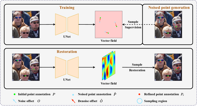
Figure 2: The pipeline of the proposed Noised Autoencoders (NAE), consisting of three parts: 1) Noised point generation by adding random noise offsets to the initial annotated points; 2) Training the NAE with generated noise offsets, restoring noised points to their original positions based on predicted vector field; 3) Self-restoration that shifts the originally annotated points with corresponding denoise offsets in the predicted vector field.

2.3 Annotation refinement

ADSCNet [2] introduces a novel framework that leverages network estimation to refine density map target using Gaussian Mixture Models (GMM). Both BL [27] and RSI [4] methodologies emphasize enhancing noise resistance in their respective frameworks. BL achieves this through the introduction of an innovative loss function, whereas RSI targets improvements via a redesigned network component. Building upon BL, NoisyCC [39] incorporates a loss function that reduces the loss weights of uncertain regions on the density map, mitigating the impact of noisy annotations.

These methods primarily focus on enhancing the model’s tolerance to annotation noise rather than directly improving the quality of the initial point annotations. Additionally, applying these methods each time incurs additional training costs. Furthermore, these methods are primarily tailored for density-based methods, which may impose limitations on their applicability to localization-based methods. In contrast, our proposed approach focus on directly refining initial point annotations, presenting a more efficient and broadly applicable solution.

3 Methodology

In this section, we present the Noised Autoencoders (NAE), a novel approach designed to enhance the consistency of point annotations in object counting datasets. The workflow of our approach is detailed in Fig. 2. We begin by explaining how the noised points are generated, then delve into a comprehensive introduction of the training and restoration steps involved in NAE.

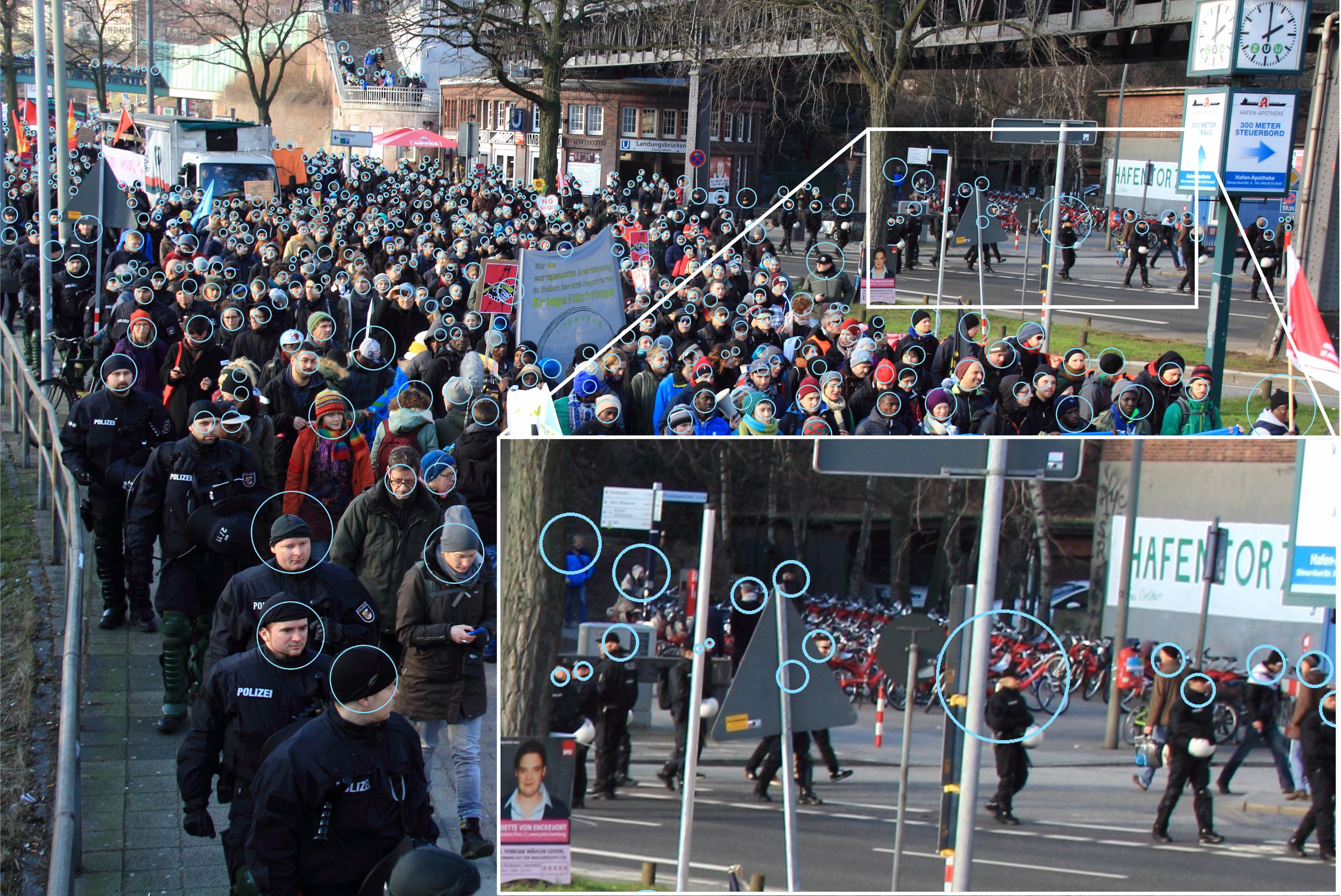
(a)

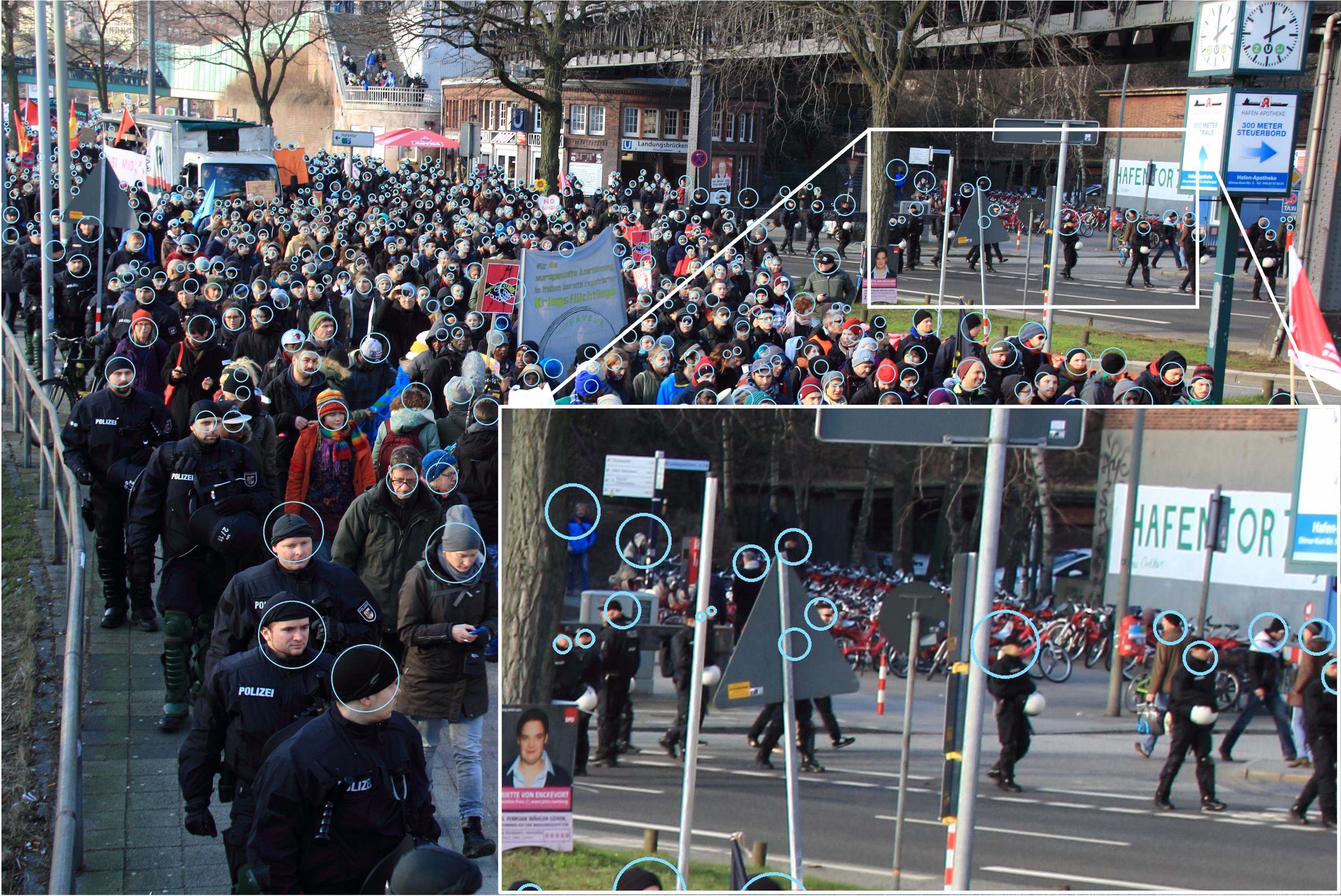
(b)

(c)

Figure 3: Illustration of different strategies to define the sampling region for each annotated point in crowd images of surveillance scene. See Eq. (3) and corresponding text for more details. Best viewed by zooming in the electronic version.

3.1 Noised point generation

Drawing inspiration from the random masking method used in MAE [11], we introduce a similar method where the initial annotations are randomly offset, and a vector field prediction is employed for their restoration.

In this section, we describe the process of generating noised points. Given an image $X$ in the training set, it is associated with a set of point annotations $P=\{{(x_{i},y_{i})}\}$, where $i$ ranges from 1 to $N$, and $N$ denotes the total number of point annotations in the image. For the $i_{th}$ point $P_{i}$ in $P$, the applied noise offset $o_{i}$ can be expressed as a two-dimensional vector, which is then decomposed into two separate components: direction $a_{i}$ and magnitude $m_{i}$. Each component is considered independently.

Direction of noise offset. The direction component $a_{i}$, which dictates the orientation of the noise offset $o_{i}$, is uniformly sampled from a full range of angles in a 2D plane. This is mathematically represented as:

$$a_{i}\sim U(0,2\pi)$$ (1)

where $U$ symbolizes a uniform distribution.

Magnitude of noise offset. To ensure that noise offsets remain within a reasonable range, the distribution range for $m_{i}$ is appropriately bounded. The magnitude component $m_{i}$ is sampled from a uniform distribution. The formulation is expressed as:

$$m_{i}\sim U(0,r_{i})$$ (2)

where $r_{i}$ represents the upper bound for $m_{i}$.

To determine $R=\{r_{i}\}$ for all points in $P$, the point set $P$ is firstly expanded to a three-dimensional format, expressed as ${\{(x_{i},y_{i},d_{i})\}}$, where the additional $d_{i}$ reflects the euclidean distance to the nearest neighboring point in $P$.

There are two critical factors to consider when setting $r_{i}$. Firstly, $r_{i}$ should be constrained to not exceed $\alpha\times d_{i}$, where $\alpha$ is a hyper-parameter to control the area of sampling, and it must be constrained to not exceed 0.5. As illustrated in Fig. 3(a), this limitation prevents the points from being offset to regions that are closer to other points.

Secondly, in crowd counting datasets [49, 14, 34], the perspective effect of the camera plays a crucial role [44]. This phenomenon results in pedestrians at different depths within the field displaying varying sizes on the image plane. Considering the physical sizes of human heads remain roughly constant, those appearing higher in the image are rendered smaller due to the perspective effect. Therefore, this phenomenon must be considered in the parameter setting for crowd counting datasets. As outlined in Algorithm 1, our method employs a sliding window approach, moving from the bottom to the top of the image. With all $r_{i}$ in each window, we select the maximum value to serve as an additional upper boundary. Moreover, this value is designed to progressively decrease as we ascend along the height of the image. This extra limitation is denoted as $L=\{{l_{j}}\}$, where $j$ ranges from $1$ to $H$ and $H$ denotes the height of the image. As highlighted in the white rectangle in Fig. 3(b), when considering both $d_{i}$ and $l_{y_{i}}$, the optimized sampling regions (blue circles) demonstrate improved alignment with the respective object scale.

However, for datasets such as remote sensing object counting [7] and cell counting [16], where there are no perspective issues, we set all values in $L$ for each image as a constant value, the median of all $d$ in this image.

Finally, the upper limitation $r_{i}$ for $m_{i}$ is as follows:

$${r_{i}=\alpha\times min(d_{i},l_{y_{i}})}$$ (3)

where $\alpha$ is a hyper-parameter to control the area of sampling, and it must be constrained to not exceed 0.5.

# Inputs:

H (Image height)

P (N*[x_coord, y_coord, radius])

# Output:

L (Upper bound for each row)

L = np.zeros(H + 1)

L[-1] = np.max(P[:, 2])

# Define the window size

winSize = H // 50

# Iterate over each row

for i in range(H - 1, -1, -1):

# Using a sliding window

win = P[P[:, 1] > i - winSize & P[:, 1] <= i + winSize]

if len(win) > 0:

maxRad = np.max(win[:, 2])

else:

maxRad = L[i + 1]

# Ensure non-increasing upwards

L[i] = min(maxRad, L[i + 1])

return L = L[:-1]

Algorithm 1 Code for computing the upper bound $L$ of sampling region’s radius for crowd images.

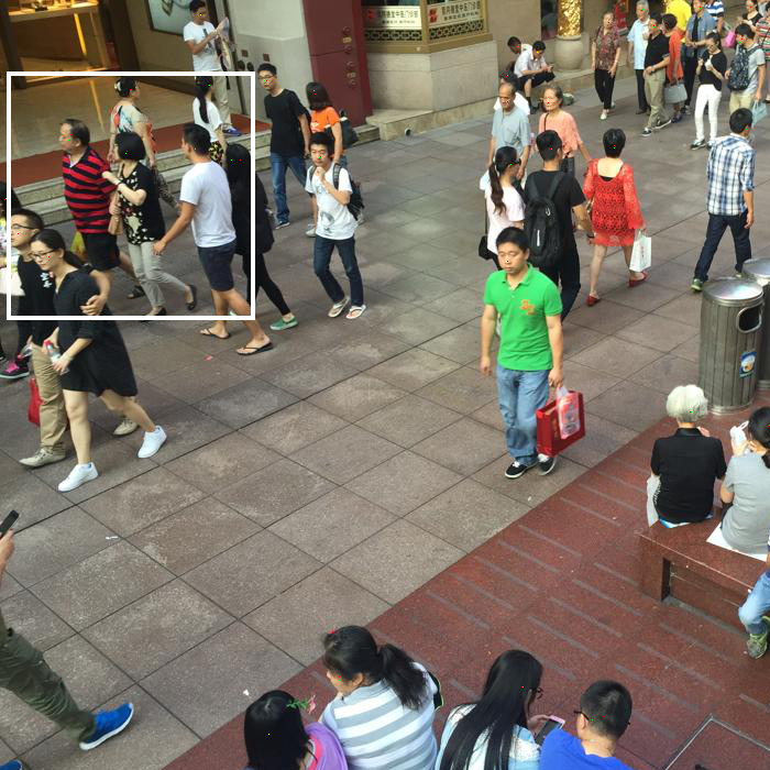
(a)

(b)

(c)

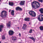
(d)

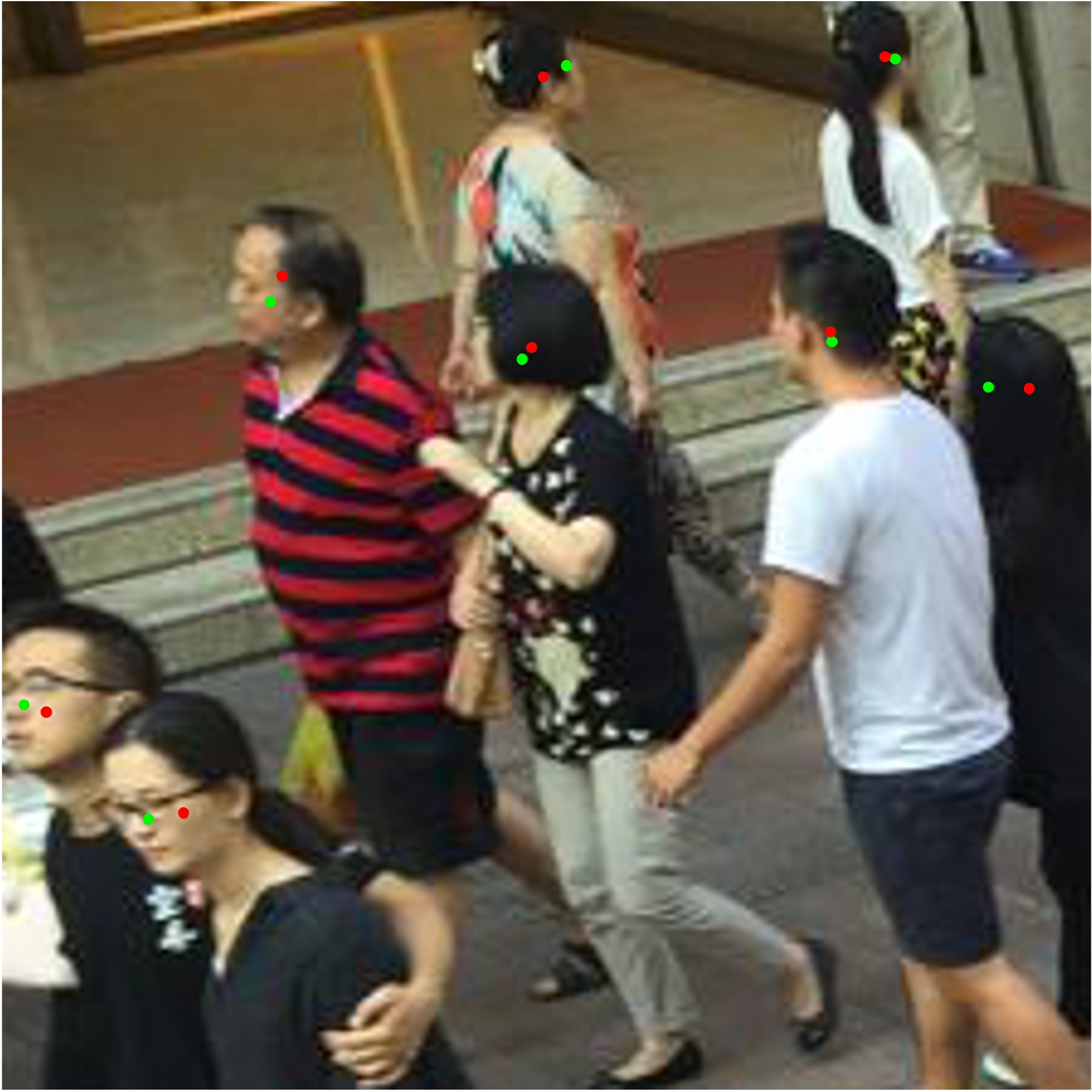
(e)

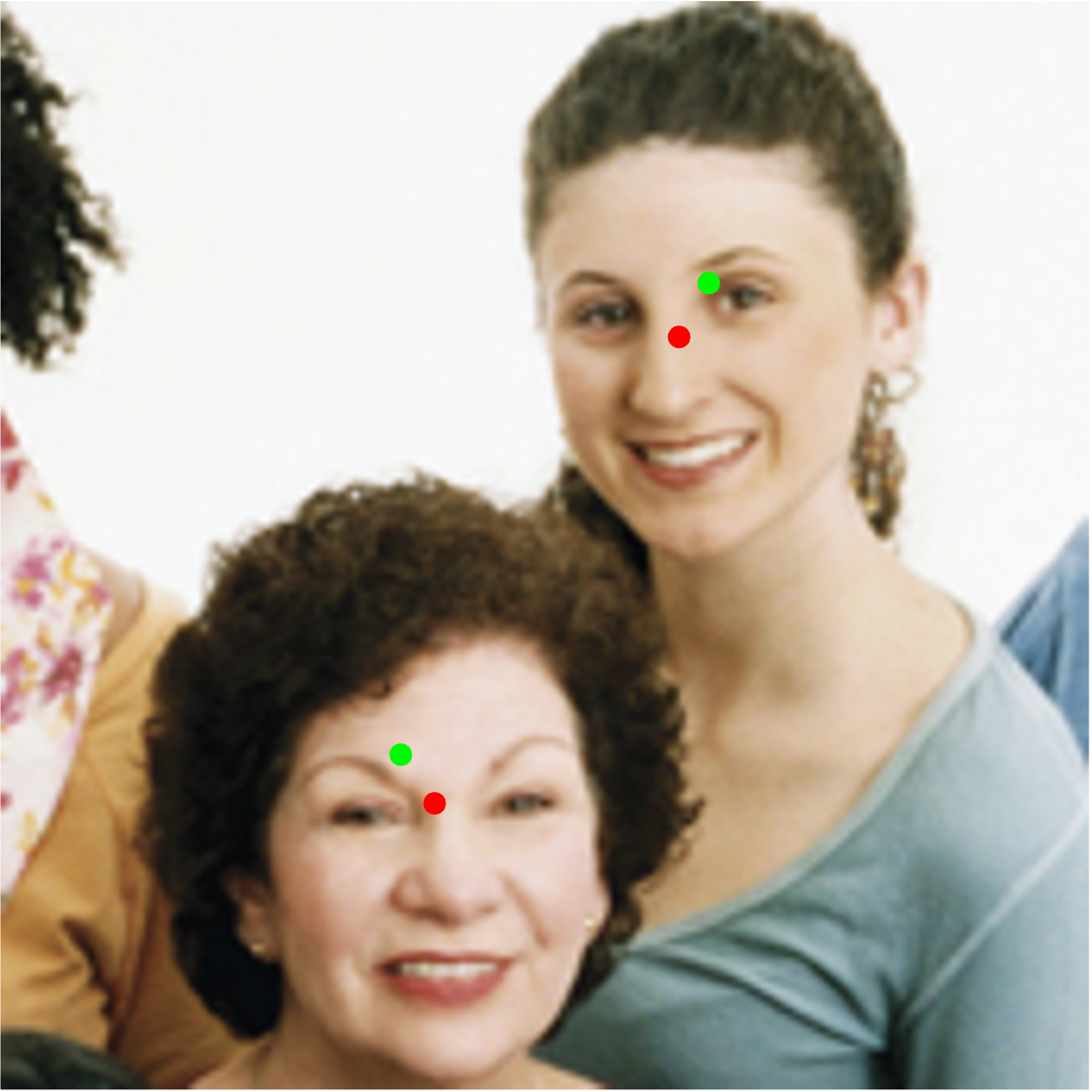
(f)

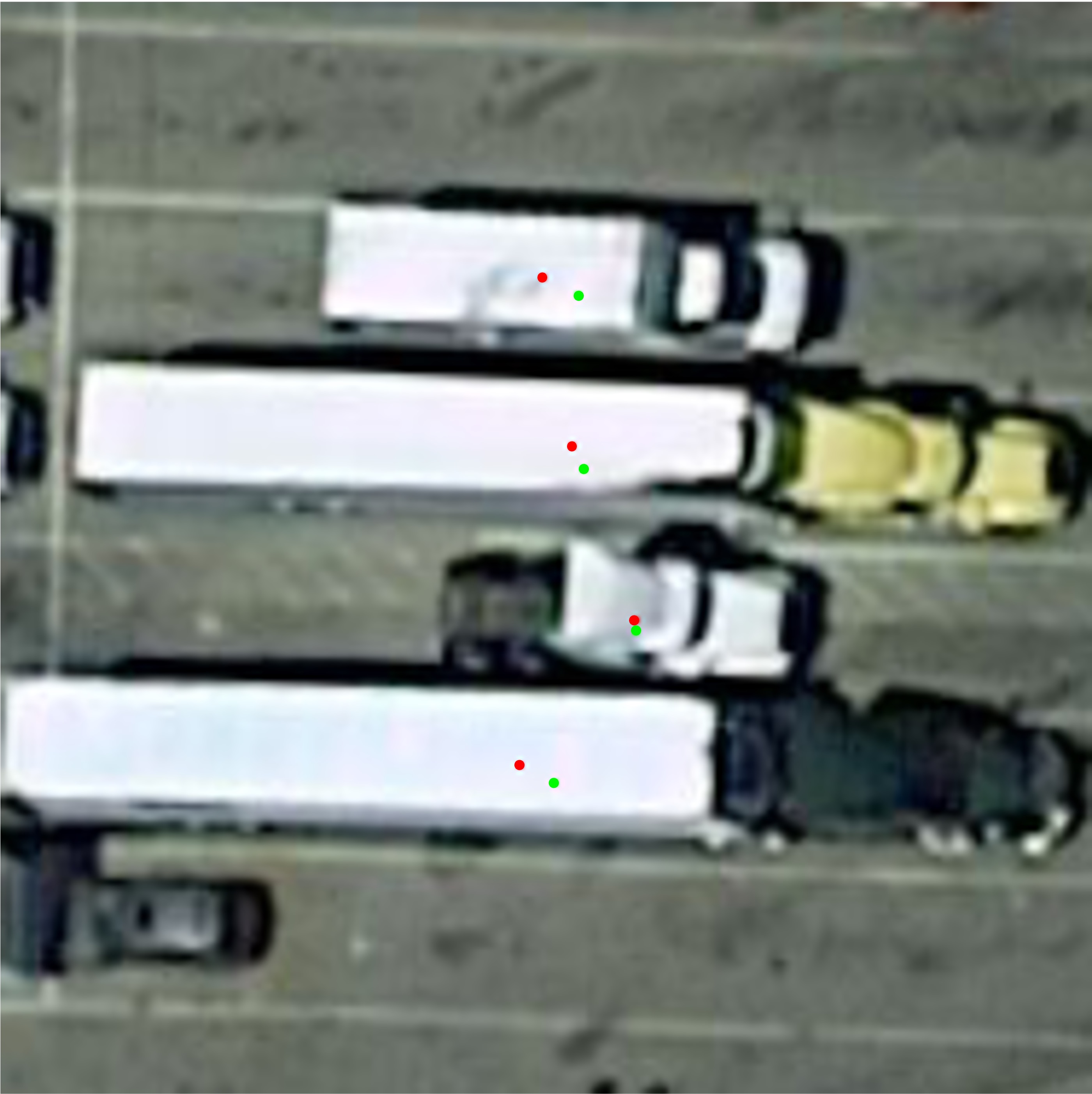
(g)

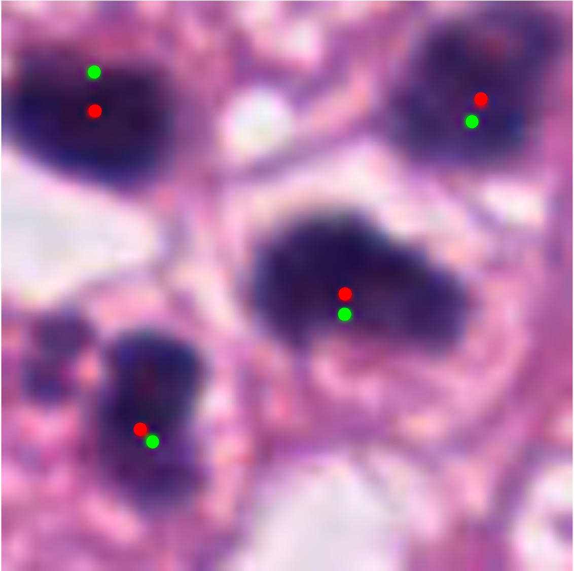
(h)

Figure 4: Visualization of restored point annotation given by the proposed NAE. The bottom row provides a zoomed-in view within the white box of the top row. Green points: initial point annotations; Red points: revised point annotations; Yellow points: initial point annotation coincides with the corresponding revised point annotation.

With the direction $d_{i}$ and the magnitude $m_{i}$, the 2D noise offset $o_{i}$ for the annotation point $P_{i}$ can be generated:

$$o_{i}=\begin{pmatrix}o_{i}^{x}\\ o_{i}^{y}\\ \end{pmatrix}=\begin{pmatrix}m_{i}\times\cos{a_{i}}\\ m_{i}\times\sin{a_{i}}\\ \end{pmatrix}$$ (4)

By imposing $o_{i}$ to the corresponding initial point, the noised point set $\hat{P}$ are obtained as follows:

$$\hat{P}=\{{(\hat{x_{i}},\hat{y_{i}})}\}=\{{(x_{i}+o_{i}^{x},y_{i}+o_{i}^{y})}\}$$ (5)

3.2 NAE network training

NAE network architecture. In our NAE network, we adopt a UNet architecture [31], incorporating with a VGG16 [33] backbone, to predict the denoise vector field $F_{2\times H\times W}$, which comprises two channels, corresponding to the $x$ and $y$ axes. The denoise vector field share same size spatially with the input image.

Training objective. In alignment with the approach adopted in MAE [11], the training of our NAE network is steered using the Mean Squared Error (MSE) loss. The process initiates by sampling within $F$ using the coordinates from the noised point set $\hat{P}$, which results in the corresponding denoise offsets denoted as $\hat{o}_{i}=\begin{pmatrix}\hat{o}_{i}^{x}\\ \hat{o}_{i}^{y}\end{pmatrix}$. The loss function is then defined as:

$$\text{Loss}=\frac{1}{N}\sum_{i=1}^{N}\left\|\hat{o}_{i}-(-o_{i})\right\|^{2}$$ (6)

where $N$ refers to the total number of point annotations in a given image within the training set.

3.3 Point annotation restoration

After the training phase, each image in the training set is processed through the trained UNet to generate the corresponding 2D vector field map $F$. During the restoration phase, the coordinates from $P$ are used to sample in the $F$, and refine each initial point annotation with the corresponding $\hat{o_{i}}$. The restoration process is defined as follows:

$$P_{r}=\{(x_{i}+\hat{o}_{i}^{x},y_{i}+\hat{o}_{i}^{y})\}$$ (7)

Through this procedure, the restored point annotations exhibit enhanced consistency compared to their original version.

4 Experiments

Table 1: Quantitative comparison of crowd counting results on the ShanghaiTech [49], UCF-QNRF [14], and JHU-Crowd++ [34] datasets. The best performance is in boldface. ${\dagger}$ represents reproduced results with official codes.

Method	SH PartA		SH PartB		UCF-QNRF		JHU-Crowd++
	MAE$\downarrow$	MSE$\downarrow$	MAE$\downarrow$	MSE$\downarrow$	MAE$\downarrow$	MSE$\downarrow$	MAE$\downarrow$	MSE$\downarrow$
CSRNet [20] (CVPR’18)	68.2	115.0	10.6	16.0	-	-	85.9	309.2
CAN [26] (CVPR’19)	62.3	100.0	7.8	12.2	107.0	183.0	100.1	314.0
ADSCNet [2] (CVPR’20)	55.4	97.7	6.4	11.3	71.3	132.5	-	-
GL [42] (CVPR’21)	61.3	95.4	7.3	11.7	84.3	147.5	59.9	259.5
CLTR [21] (ECCV’22)	56.9	95.2	6.5	10.6	85.8	141.3	59.5	240.6
NoisyCC [43] (TPAMI’23)	61.8	104.3	7.1	12.4	83.8	147.8	59.1	259.6
NoisyCC [43] & MAN (TPAMI’23)	56.4	89.4	6.5	10.3	75.3	128.3	53.0	208.6
CrowdHat [45] (CVPR’23)	51.2	81.9	5.7	9.4	75.1	126.7	52.3	211.8
AWCCNet [13] (ICCV’23)	56.2	91.3	-	-	76.4	130.5	52.3	207.2
PET [25] (ICCV’23)	49.3	78.8	6.2	9.7	79.5	144.3	58.5	238.0
BL† [27] (ICCV’19)	62.7	99.5	7.6	13.00	87.4	149.6	74.4	290.0
BL & NAE	61.6 ($\downarrow$1.1)	96.9 ($\downarrow$2.6)	7.2 ($\downarrow$0.4)	11.9 ($\downarrow$1.1)	83.7 ($\downarrow$3.7)	146.5 ($\downarrow$3.1)	58.6 ($\downarrow$15.8)	234.9 ($\downarrow$55.1)
NoisyCC† [39] (NeurIPS’20)	62.1	100.0	7.5	11.4	86.1	149.7	67.5	255.4
NoisyCC & NAE	60.6 ($\downarrow$1.5)	95.4 ($\downarrow$4.6)	6.9 ($\downarrow$0.6)	11.7 ($\uparrow$0.3)	82.1 ($\downarrow$4.0)	148.4 ($\downarrow$1.3)	58.6 ($\downarrow$8.9)	231.8 ($\downarrow$23.6)
RSI-ResNet50† [4] (CVPR’22)	54.4	89.0	6.6	9.8	81.2	152.0	58.8	245.1
RSI-ResNet50 & NAE	52.8 ($\downarrow$1.6)	86.1 ($\downarrow$2.9)	5.8 ($\downarrow$0.8)	8.9 ($\downarrow$0.9)	78.4 ($\downarrow$2.8)	145.6 ($\downarrow$6.4)	55.1 ($\downarrow$3.7)	239.7 ($\downarrow$5.4)
P2PNet† [35] (ICCV’21)	52.8	85.8	6.5	10.9	91.7	157.0	64.3	253.1
P2PNet & NAE	48.3 ($\downarrow$4.5)	75.8 ($\downarrow$10.0)	6.1 ($\downarrow$0.4)	9.8 ($\downarrow$1.1)	86.0 ($\downarrow$5.7)	148.7 ($\downarrow$8.3)	62.6 ($\downarrow$1.7)	244.5 ($\downarrow$8.6)
MAN† [24] (CVPR’22)	56.8	90.2	7.1	10.5	77.5	132.7	53.2	219.9
MAN & NAE	52.9 ($\downarrow$3.9)	84.9 ($\downarrow$5.3)	5.5 ($\downarrow$1.6)	8.1 ($\downarrow$2.4)	74.2 ($\downarrow$3.3)	125.6 ($\downarrow$7.1)	48.6 ($\downarrow$4.6)	202.8 ($\downarrow$17.1)
STEERER† [10] (ICCV’23)	56.5	89.8	7.1	10.7	74.1	129.5	55.8	223.2
STEERER & NAE	55.1 ($\downarrow$1.4)	85.5 ($\downarrow$4.3)	6.4 ($\downarrow$0.7)	10.2 ($\downarrow$0.5)	72.4 ($\downarrow$1.7)	125.4 ($\downarrow$4.1)	53.7 ($\downarrow$2.1)	214.3 ($\downarrow$8.9)

4.1 Experimental setting

Datasets. To evaluate the effectiveness of the proposed approach, we perform extensive experiments on eleven datasets spanning three domains: crowd counting, remote sensing object counting, and cell counting. These datasets include: SH PartA [49], SH PartB [49], UCF-QNRF [14], JHU++ [34], RSOC_building [7], RSOC_small-vehicle [7], RSOC_large-vehicle [7], RSOC_ship [7], MBM [16], ADI [29], and DCC [28].

Evaluation metrics. In object counting tasks, the Mean Absolute Error (MAE) and Mean Square Error (MSE) serve as the principal evaluation metrics. Lower values for these metrics indicate better performance.

Implementation details. During the training phase for NAE, we augment the images with random scaling and horizontal flipping. The images are then randomly cropped to a size of $512\times 512$ pixels, except for the ADI dataset [29], where a crop size of $128\times 128$ pixels is adopted due to the limited resolution. Additionally, we randomly regenerate the noise offset for images in each iteration.

We utilize the Adam optimizer for training, setting a weight decay of $5\times 10^{-4}$ and maintaining a constant learning rate of $10^{-4}$. The training is executed in the PyTorch framework, utilizing a RTX 3090 GPU. For each dataset, the training spans 100 epochs with a batch-size of 8.

4.2 Experimental results

Our experimental evaluation encompasses eleven publicly available datasets across three different domains: crowd counting, remote sensing object counting, and cell counting. Fig. 4 presents some qualitative results, illustrating the NAE’s effectiveness in improving the consistency of point annotations for various object types. We perform quantitative comparisons by training existing methods with initial and refined annotations, respectively. As detailed in Sec. 4.2.1, we demonstrate the robustness of our NAE under conditions where extra noise is added to the initial annotations for crowd counting. Subsequent sections provide detailed quantitative comparisons for each of the three domains under normal situation.

4.2.1 Robustness against noisy point annotations

This section assesses the robustness of NAE against noisy point annotations, a common issue in manual annotation processes. We emulate real-world annotation errors by introducing varying offsets to each annotation point $P_{i}$. The magnitude of offsets are set to $0.2\cdot d$, $0.4\cdot d$, $0.6\cdot d$, and $0.8\cdot d$ pixels, where $d$ represents the nearest distance to other points. This strategy effectively evaluates NAE’s performance in managing the inaccuracies typically present in manual annotations.

The analysis compares various methodologies, including BL [27], NoiseCC [39], and BL & NAE, on UCF-QNRF [14] with artificially induced point annotation noise. As shown in Fig. 5, increasing noise levels pose a challenge to all methods in maintaining accuracy. Remarkably, NAE consistently outperforms other techniques, achieving lower Mean Absolute Error (MAE). These findings emphasize NAE’s effectiveness in handling noisy and imperfect point annotation, a common occurrence in real-world counting tasks.

Figure 5: Quantitative evaluation of robustness to different synthetic noise levels applied to original point annotation.

Table 2: Quantitative comparison of remote sensing object counting results on the RSOC datasets [7]. The best performance is in boldface. ${\dagger}$ represents reproduced results with official codes.

Method	RSOC_Building		RSOC_Small-vehicle		RSOC_Large-vehicle		RSOC_Ship
	MAE$\downarrow$	MSE$\downarrow$	MAE$\downarrow$	MSE$\downarrow$	MAE$\downarrow$	MSE$\downarrow$	MAE$\downarrow$	MSE$\downarrow$
MCFA [6] (TGRS’21)	7.9	11.8	238.5	625.9	12.9	20.3	50.5	65.2
ADMAL [5] (TGRS’22)	5.6	7.7	115.6	210.8	11.7	17.3	45.1	64.8
eFreeNet [12] (TGRS’23)	5.6	7.7	195.9	463.6	14.6	19.8	65.3	85.5
LMSFFNet [48] (TGRS’23)	6.3	9.4	141.7	273.0	12.7	27.1	49.5	70.0
BL† [27] (ICCV’19)	11.5	16.3	109.9	353.9	12.3	24.2	58.8	195.5
BL & NAE	11.1 ($\downarrow$0.4)	15.7 ($\downarrow$0.6)	86.7 ($\downarrow$23.2)	197.0 ($\downarrow$156.9)	9.7 ($\downarrow$2.6)	18.4 ($\downarrow$5.8)	50.8 ($\downarrow$8.0)	128.1 ($\downarrow$67.4)
NoisyCC† [39] (NeurIPS’20)	7.8	11.3	168.8	529.1	15.5	31.4	53.0	72.1
NoisyCC & NAE	7.4 ($\downarrow$0.4)	10.2 ($\downarrow$1.1)	145.3 ($\downarrow$23.5)	401.4 ($\downarrow$127.7)	14.6 ($\downarrow$0.9)	28.7 ($\downarrow$2.7)	47.9 ($\downarrow$5.1)	70.4 ($\downarrow$1.7)
P2PNet† [35] (ICCV’21)	6.3	9.1	102.5	238.9	8.1	13.2	28.2	42.6
P2PNet & NAE	5.6 ($\downarrow$0.7)	8.1 ($\downarrow$1.0)	96.2 ($\downarrow$6.3)	237.0 ($\downarrow$1.9)	7.0 ($\downarrow$1.1)	11.3 ($\downarrow$1.9)	25.2 ($\downarrow$3.0)	39.3 ($\downarrow$3.3)
ASPDNet† [7] (TGRS’20)	7.6	11.5	252.6	718.5	19.7	27.8	81.8	110.3
ASPDNet & NAE	6.7 ($\downarrow$0.9)	10.5 ($\downarrow$1.0)	208.9 ($\downarrow$43.7)	293.4 ($\downarrow$425.1)	15.3 ($\downarrow$4.4)	22.2 ($\downarrow$5.6)	72.3 ($\downarrow$9.5)	95.8 ($\downarrow$14.5)
PSGCNet† [8] (TGRS’22)	7.4	11.1	112.1	289.6	11.8	16.4	39.5	68.5
PSGCNet & NAE	6.3 ($\downarrow$1.1)	10.1 ($\downarrow$1.0)	101.6 ($\downarrow$10.5)	237.0 ($\downarrow$52.6)	9.6 ($\downarrow$2.2)	13.9 ($\downarrow$2.5)	35.3 ($\downarrow$4.2)	64.4 ($\downarrow$4.1)

4.2.2 Crowd counting

Comparison with state-of-the-art methods. We conduct a comprehensive evaluation of the NAE-refined point annotations compared with the initial ones, employing a variety of SOTA density-map-based and localization-based crowd counting models. The quantitative results, depicted in Tab. 1, demonstrate the effectiveness of NAE on various baseline methods. A notable improvement is observed when applied to P2PNet [35], where NAE achieves a reduction of 5.7 in Mean Absolute Error (MAE) and 8.3 in Mean Squared Error (MSE) on UCF-QNRF dataset. Remarkably, the integration of NAE leads to the establishment of new state-of-the-art results in three of the four assessed datasets: SH PartA [49], SH PartB [49], and JHU++ [34]. On average, NAE contributes to an reduction of 2.6 in MAE and 6.5 in MSE compared to the results of three baseline methods (P2PNet [35], MAN [24], and STEERER [10]) on the four extensively used datasets.

Effectiveness on anti-noise methods. Further inverstigation are conducted to assess NAE’s compatibility with those anti-noise approaches: BL [27], NoisyCC [39], and RSI [4]. While these methods primarily focus on improving noise resilience, they do not inherently improve the intrinsic quality of point annotations. As exhibited in Tab. 1, NAE further steadily improves these anti-noise frameworks, yielding an average enhancement of 3.7 in MAE and 8.9 in MSE across the four diverse datasets.

4.2.3 Remote sensing object counting

Comparison with state-of-the-art methods. In contrast to crowd counting datasets, remote sensing object counting datasets present a different challenge with their diversity, encompassing four distinct types of objects. We apply NAE to several state-of-the-art remote sensing object counting methods. The quantitative results, detailed in Tab. 2, clearly demonstrate the effective performance of NAE. It not only consistently outperforms baseline methods but also sets new state-of-the-art results in three of the four datasets: RSOC_Small-vehicle, RSOC_Large-vehicle, and RSOC_Ship [7]. Notably, NAE achieves, on average, an improvement of 7.3 in Mean Absolute Error (MAE) and 42.9 in Mean Squared Error (MSE) over the three baseline models (P2PNet [35], ASPDNet [7], and PSGCNet [8]) across these four datasets.

Effectiveness on anti-noise methods. In addition to state-of-the-art approaches, we also examine the effectiveness of our method on two anti-noise methods, BL [27] and NoisyCC [39]. These anti-noise methods aim to enhance the model’s noise resilience, primarily through adjustments in the loss functions. The comparative results shown in Tab. 2 reveal that NAE can further augment these anti-noise methods, resulting in an average improvement of 8.0 in MAE and 45.5 in MSE across the four datasets.

Table 3: Quantitative comparison of cell counting results on the MBM [16], ADI [29], and DCC [28] datasets. The best performance is in boldface. ${\dagger}$ represents reproduced results.

Method	MBM		ADI		DCC
	MAE$\downarrow$	MSE$\downarrow$	MAE$\downarrow$	MSE$\downarrow$	MAE$\downarrow$	MSE$\downarrow$
BL† [27]	8.4	10.3	13.7	18.7	3.3	5.3
BL & NAE	6.4	7.7	13.1	17.7	2.9	4.9
NoisyCC† [39]	7.2	9.3	14.0	18.8	3.8	5.6
NoisyCC & NAE	6.0	8.6	13.1	17.9	3.6	5.4
P2PNet† [35]	5.7	8.0	12.4	17.1	3.7	6.0
P2PNet & NAE	4.6	5.9	11.8	16.6	3.2	5.5
Chen et al.† [3] 2020	5.6	8.3	12.7	19.6	5.7	7.6
Chen et al. & NAE	4.6	7.5	11.1	15.8	4.7	7.1
SAUNet† [9] 2022	5.7	7.7	14.3	18.5	3.0	4.8
SAUNet & NAE	4.2	5.6	10.8	13.9	2.4	3.3

4.2.4 Cell counting

Comparison with state-of-the-art methods. The proposed NAE method extends its utility beyond natural image datasets, demonstrating its ability to resolve annotation inconsistency challenges encountering in medical counting datasets. As detailed in Tab. 3, NAE’s effectiveness in boosting cell counting methods through improving annotation ability is consistent. We establish new state-of-the-art records across all the three cell counting datasets. Notably, with SAU [9] already achieving excellent results on DCC [28] with an MAE of 3 and an MSE of 4.8, the integration of NAE further enhances the performance, reducing the MAE to 2.4 and MSE to 3.3, respectively.

Effectiveness on anti-noise methods. Additionally, we also explore NAE’s universal applicability in conjunction with two established anti-noise methods: BL [27] and NoisyCC [39]. These two methods focus on improving noise robustness by introducing novel loss functions. However, the proposed NAE can consistently improve their performance, which further validates its effectiveness.

Table 4: Quantitative results of BL [27] on UCF-QNRF [14], RSOC Small-vehicle (RSV) [7], and MBM [16] dataset with NAE using different values of $\alpha$ involved in Eq. (3).

$\alpha$	UCF-QNRF		RSV		MBM
	MAE$\downarrow$	MSE$\downarrow$	MAE$\downarrow$	MSE$\downarrow$	MAE$\downarrow$	MSE$\downarrow$
Baseline	87.4	149.6	109.9	353.9	8.4	10.3
0.3	85.7	152.2	87.1	214.0	7.0	9.1
0.4	83.7	146.5	86.7	197.0	6.4	7.7
0.5	83.9	148.1	86.9	201.6	7.3	9.2
0.6	90.4	156.7	112.5	366.2	9.0	11.7

4.3 Ablation study

Analysis of Hyper-Parameter $\alpha$ in Eq. (3). As delineated in Eq. (3), the hyper-parameter $\alpha$ plays a crucial role in defining the sample area. A smaller value of $\alpha$ leads to a more constrained sample range, which may reduce the NAE model’s effectiveness in refining annotations with high deviation from their ideal positions. In contrast, a larger $\alpha$ tends to include more background regions within the sample range. Notably, when the sampling areas for different annotation points overlap, it leads to ambiguity. This overlap challenges NAE’s ability to distinguish between regions associated with distinct objects.

To evaluate the impact of the hyper-parameter $\alpha$ on our model’s performance, we conduct an ablation study with $\alpha$ values set at 0.3, 0.4, 0.5, and 0.6. This study utilizes the Bayesian Loss (BL) [27], and covers three diverse datasets: UCF-QNRF [14], Remote_small-vehicle [7], and MBM [16]. These datasets represent crowd counting, remote sensing object counting, and cell counting scenarios, respectively. The results, presented in Tab. 4, show how different $\alpha$ values influence counting accuracy. Generally, in configurations that avoid overlap, we observe enhancements in performance compared to baseline methods. However, at an $\alpha$ setting of 0.6, the overlapping sampling ranges for different objects introduce confusion in the training process, leading to performance that falls short of the baseline.

Pretraining backbone of NAE for Object Counting. Drawing inspiration from the Masked Autoencoder (MAE) approach  [11], we explore the effectiveness of using the NAE pretrained backbone for object counting. In our study, we compare our approach with two existing methods that utilize the same VGG16 backbone as NAE, namely P2PNet[35] and CSRNet [20]. We conducte an ablation study to assess the impact of the NAE pretrained backbone on these methods.

As indicated in Tab. 5, equipping both methods with the NAE backbone results in consistent performance improvements. Further enhancements in model performance are achieved when combining the revised annotations provided by NAE. Specifically, P2PNet, when augmented with both the NAE revised annotations and the NAE pretrained backbone, achieves the most significant improvement on the SH PartA dataset [49]. The Mean Absolute Error (MAE) and Mean Squared Error (MSE) decreased to 47.68 and 74.58, respectively. This study demonstrates the effectiveness of our NAE methodology in the context of object counting.

Table 5: Validation experimental results of using pretraining backbone of NAE. Ref: Refined point annotations; Pre: Pretraining.

Method	CSRNet [20]		P2PNet [35]
	MAE$\downarrow$	MSE$\downarrow$	MAE$\downarrow$	MSE$\downarrow$
Baseline	64.0	110.3	52.8	85.8
+ Res	58.6 ($\downarrow$5.4)	97.6 ($\downarrow$12.7)	48.3 ($\downarrow$4.5)	75.8 ($\downarrow$10.0)
+ Pre	59.6 ($\downarrow$4.4)	100.4 ($\downarrow$9.9)	49.4 ($\downarrow$3.4)	80.7 ($\downarrow$5.1)
+ Res & Pre	56.7 ($\downarrow$7.3)	96.1 ($\downarrow$14.2)	47.7 ($\downarrow$5.1)	74.6 ($\downarrow$11.2)

4.4 Limitation

As described in Sec. 3.1, for datasets with varying object sizes (e.g., remote sensing objects), the proposed approach adopts the median distance to the nearest object within each image to limit the offset magnitude. Though this strategy is functional, there may be more elegant and effective strategy for setting the upper bound $L$ involved in Sec. 3.1.

5 Conclusion

In this paper, we focus on the inconsistency problem of point annotations in object counting task. This is often caused by the inevitable subjective nature of annotators. To mitigate this issue, we propose the novel Noised Autoencoders (NAE) method inspired by MAE to revise the initial point annotations. Extensive experiments on eleven datasets from three different object counting tasks verify the effectiveness of the proposed NAE. Besides, based on the proposed NAE, we set new state-of-the-art results on nine of the eleven datasets. We hope that this work could shed light on research direction of directly refining the annotation in point-based vision tasks.

References

- Arteta et al. [2014] Carlos Arteta, Victor Lempitsky, J Alison Noble, and Andrew Zisserman. Interactive object counting. In Proc. of European Conf. on Computer Vision, pages 504–518, 2014.
- Bai et al. [2020] Shuai Bai, Zhiqun He, Yu Qiao, Hanzhe Hu, Wei Wu, and Junjie Yan. Adaptive dilated network with self-correction supervision for counting. In Proc. of IEEE Conf. on Computer Vision and Pattern Recognition, 2020.
- Chen et al. [2021] Yajie Chen, Dingkang Liang, Xiang Bai, Yongchao Xu, and Xin Yang. Cell localization and counting using direction field map. IEEE Journal of Biomedical and Health Informatics, 26(1):359–368, 2021.
- Cheng et al. [2022] Zhi-Qi Cheng, Qi Dai, Hong Li, Jingkuan Song, Xiao Wu, and Alexander G Hauptmann. Rethinking spatial invariance of convolutional networks for object counting. In Proc. of IEEE Conf. on Computer Vision and Pattern Recognition, pages 19638–19648, 2022.
- Ding et al. [2022] Guanchen Ding, Mingpeng Cui, Daiqin Yang, Tao Wang, Sihan Wang, and Yunfei Zhang. Object counting for remote-sensing images via adaptive density map-assisted learning. IEEE Transactions on Geoscience and Remote Sensing, 60:1–11, 2022.
- Duan et al. [2021] Zuodong Duan, Shunzhou Wang, Huijun Di, and Jiahao Deng. Distillation remote sensing object counting via multi-scale context feature aggregation. IEEE Transactions on Geoscience and Remote Sensing, 60:1–12, 2021.
- Gao et al. [2020] Guangshuai Gao, Qingjie Liu, and Yunhong Wang. Counting from sky: A large-scale data set for remote sensing object counting and a benchmark method. IEEE Transactions on Geoscience and Remote Sensing, 59(5):3642–3655, 2020.
- Gao et al. [2022] Guangshuai Gao, Qingjie Liu, Zhenghui Hu, Lu Li, Qi Wen, and Yunhong Wang. PSGCNet: A pyramidal scale and global context guided network for dense object counting in remote-sensing images. IEEE Transactions on Geoscience and Remote Sensing, 60:1–12, 2022.
- Guo et al. [2021] Yue Guo, Oleh Krupa, Jason Stein, Guorong Wu, and Ashok Krishnamurthy. Sau-net: A unified network for cell counting in 2d and 3d microscopy images. IEEE/ACM transactions on computational biology and bioinformatics, 19(4):1920–1932, 2021.
- Han et al. [2023] Tao Han, Lei Bai, Lingbo Liu, and Wanli Ouyang. STEERER: Resolving scale variations for counting and localization via selective inheritance learning. In Proc. of IEEE Intl. Conf. on Computer Vision, pages 21848–21859, 2023.
- He et al. [2022] Kaiming He, Xinlei Chen, Saining Xie, Yanghao Li, Piotr Dollár, and Ross Girshick. Masked autoencoders are scalable vision learners. In Proc. of IEEE Conf. on Computer Vision and Pattern Recognition, pages 16000–16009, 2022.
- Huang et al. [2023a] Yongbo Huang, Yuanpei Jin, Liqiang Zhang, and Yishu Liu. Remote sensing object counting through regression ensembles and learning to rank. IEEE Transactions on Geoscience and Remote Sensing, 2023a.
- Huang et al. [2023b] Zhi-Kai Huang, Wei-Ting Chen, Yuan-Chun Chiang, Sy-Yen Kuo, and Ming-Hsuan Yang. Counting crowds in bad weather. In Proc. of IEEE Intl. Conf. on Computer Vision, pages 23308–23319, 2023b.
- Idrees et al. [2018a] Haroon Idrees, Muhmmad Tayyab, Kishan Athrey, Dong Zhang, Somaya Al-Maadeed, Nasir Rajpoot, and Mubarak Shah. Composition loss for counting, density map estimation and localization in dense crowds. In Proc. of European Conf. on Computer Vision, pages 532–546, 2018a.
- Idrees et al. [2018b] Haroon Idrees, Muhmmad Tayyab, Kishan Athrey, Dong Zhang, Somaya Al-Maadeed, Nasir Rajpoot, and Mubarak Shah. Composition loss for counting, density map estimation and localization in dense crowds. In Proc. of European Conf. on Computer Vision, pages 532–546, 2018b.
- Kainz et al. [2015] Philipp Kainz, Martin Urschler, Samuel Schulter, Paul Wohlhart, and Vincent Lepetit. You should use regression to detect cells. In Proc. of Intl. Conf. on Medical Image Computing and Computer Assisted Intervention, pages 276–283, 2015.
- Kuhn [1955] Harold W Kuhn. The hungarian method for the assignment problem. Naval research logistics quarterly, 2(1-2):83–97, 1955.
- Li et al. [2014a] Teng Li, Huan Chang, Meng Wang, Bingbing Ni, Richang Hong, and Shuicheng Yan. Crowded scene analysis: A survey. IEEE transactions on circuits and systems for video technology, 25(3):367–386, 2014a.
- Li et al. [2014b] Teng Li, Huan Chang, Meng Wang, Bingbing Ni, Richang Hong, and Shuicheng Yan. Crowded scene analysis: A survey. IEEE transactions on circuits and systems for video technology, 25(3):367–386, 2014b.
- Li et al. [2018] Yuhong Li, Xiaofan Zhang, and Deming Chen. Csrnet: Dilated convolutional neural networks for understanding the highly congested scenes. In Proc. of IEEE Conf. on Computer Vision and Pattern Recognition, pages 1091–1100, 2018.
- Liang et al. [2022a] Dingkang Liang, Wei Xu, and Xiang Bai. An end-to-end transformer model for crowd localization. In Proc. of European Conf. on Computer Vision, pages 38–54, 2022a.
- Liang et al. [2022b] Dingkang Liang, Wei Xu, Yingying Zhu, and Yu Zhou. Focal inverse distance transform maps for crowd localization. IEEE Trans. on Multimedia, 2022b.
- Liang et al. [2023] Dingkang Liang, Jiahao Xie, Zhikang Zou, Xiaoqing Ye, Wei Xu, and Xiang Bai. Crowdclip: Unsupervised crowd counting via vision-language model. In Proc. of IEEE Conf. on Computer Vision and Pattern Recognition, pages 2893–2903, 2023.
- Lin et al. [2022] Hui Lin, Zhiheng Ma, Rongrong Ji, Yaowei Wang, and Xiaopeng Hong. Boosting crowd counting via multifaceted attention. In Proc. of IEEE Conf. on Computer Vision and Pattern Recognition, pages 19628–19637, 2022.
- Liu et al. [2023] Chengxin Liu, Hao Lu, Zhiguo Cao, and Tongliang Liu. Point-Query quadtree for crowd counting, localization, and more. In Proc. of IEEE Intl. Conf. on Computer Vision, pages 1676–1685, 2023.
- Liu et al. [2019] Weizhe Liu, Mathieu Salzmann, and Pascal Fua. Context-aware crowd counting. In Proc. of IEEE Conf. on Computer Vision and Pattern Recognition, pages 5099–5108, 2019.
- Ma et al. [2019] Zhiheng Ma, Xing Wei, Xiaopeng Hong, and Yihong Gong. Bayesian loss for crowd count estimation with point supervision. In Proc. of IEEE Intl. Conf. on Computer Vision, pages 6142–6151, 2019.
- Marsden et al. [2018] Mark Marsden, Kevin McGuinness, Suzanne Little, Ciara E Keogh, and Noel E O’Connor. People, penguins and petri dishes: Adapting object counting models to new visual domains and object types without forgetting. In Proc. of IEEE Conf. on Computer Vision and Pattern Recognition, pages 8070–8079, 2018.
- Paul Cohen et al. [2017] Joseph Paul Cohen, Genevieve Boucher, Craig A Glastonbury, Henry Z Lo, and Yoshua Bengio. Count-ception: Counting by fully convolutional redundant counting. In Proc. of IEEE Intl. Conf. on Computer Vision Workshops, pages 18–26, 2017.
- Reynolds et al. [2009] Douglas A Reynolds et al. Gaussian mixture models. Encyclopedia of biometrics, 741(659-663), 2009.
- Ronneberger et al. [2015] Olaf Ronneberger, Philipp Fischer, and Thomas Brox. U-net: Convolutional networks for biomedical image segmentation. In Proc. of Intl. Conf. on Medical Image Computing and Computer Assisted Intervention, pages 234–241, 2015.
- Sam et al. [2020] Deepak Babu Sam, Skand Vishwanath Peri, Mukuntha Narayanan Sundararaman, Amogh Kamath, and R Venkatesh Babu. Locate, size, and count: accurately resolving people in dense crowds via detection. IEEE Trans. on Pattern Anal. and Mach. Intell., 43(8):2739–2751, 2020.
- Simonyan and Zisserman [2014] Karen Simonyan and Andrew Zisserman. Very deep convolutional networks for large-scale image recognition. arXiv preprint arXiv:1409.1556, 2014.
- Sindagi et al. [2020] Vishwanath A Sindagi, Rajeev Yasarla, and Vishal M Patel. Jhu-crowd++: Large-scale crowd counting dataset and a benchmark method. IEEE Trans. on Pattern Anal. and Mach. Intell., 44(5):2594–2609, 2020.
- Song et al. [2021a] Qingyu Song, Changan Wang, Zhengkai Jiang, Yabiao Wang, Ying Tai, Chengjie Wang, Jilin Li, Feiyue Huang, and Yang Wu. Rethinking counting and localization in crowds: A purely point-based framework. In Proc. of IEEE Intl. Conf. on Computer Vision, pages 3365–3374, 2021a.
- Song et al. [2021b] Qingyu Song, Changan Wang, Yabiao Wang, Ying Tai, Chengjie Wang, Jilin Li, Jian Wu, and Jiayi Ma. To choose or to fuse? scale selection for crowd counting. In Proc. of the AAAI Conf. on Artificial Intelligence, pages 2576–2583, 2021b.
- Sun et al. [2023] Guolei Sun, Zhaochong An, Yun Liu, Ce Liu, Christos Sakaridis, Deng-Ping Fan, and Luc Van Gool. Indiscernible object counting in underwater scenes. In Proc. of IEEE Conf. on Computer Vision and Pattern Recognition, pages 13791–13801, 2023.
- Wan and Chan [2019] Jia Wan and Antoni Chan. Adaptive density map generation for crowd counting. In Proc. of IEEE Intl. Conf. on Computer Vision, pages 1130–1139, 2019.
- Wan and Chan [2020] Jia Wan and Antoni Chan. Modeling noisy annotations for crowd counting. Proc. of Advances in Neural Information Processing Systems, 33:3386–3396, 2020.
- Wan et al. [2020] Jia Wan, Qingzhong Wang, and Antoni B Chan. Kernel-based density map generation for dense object counting. IEEE Trans. on Pattern Anal. and Mach. Intell., 44(3):1357–1370, 2020.
- Wan et al. [2021a] Jia Wan, Nikil Senthil Kumar, and Antoni B Chan. Fine-grained crowd counting. IEEE Trans. on Image Processing, 30:2114–2126, 2021a.
- Wan et al. [2021b] Jia Wan, Ziquan Liu, and Antoni B Chan. A generalized loss function for crowd counting and localization. In Proc. of IEEE Conf. on Computer Vision and Pattern Recognition, pages 1974–1983, 2021b.
- Wan et al. [2023] Jia Wan, Qiangqiang Wu, and Antoni B Chan. Modeling noisy annotations for point-wise supervision. IEEE Trans. on Pattern Anal. and Mach. Intell., 2023.
- Wu et al. [2019] Junfeng Wu, Zhiyang Li, Wenyu Qu, and Yizhi Zhou. One shot crowd counting with deep scale adaptive neural network. Electronics, 8(6):701, 2019.
- Wu and Yang [2023] Shaokai Wu and Fengyu Yang. Boosting detection in crowd analysis via underutilized output features. In Proc. of IEEE Conf. on Computer Vision and Pattern Recognition, pages 15609–15618, 2023.
- Xu et al. [2019] Chenfeng Xu, Kai Qiu, Jianlong Fu, Song Bai, Yongchao Xu, and Xiang Bai. Learn to scale: Generating multipolar normalized density maps for crowd counting. In Proc. of IEEE Intl. Conf. on Computer Vision, pages 8382–8390, 2019.
- Xu et al. [2022] Chenfeng Xu, Dingkang Liang, Yongchao Xu, Song Bai, Wei Zhan, Xiang Bai, and Masayoshi Tomizuka. Autoscale: learning to scale for crowd counting. International Journal of Computer Vision, 130(2):405–434, 2022.
- Yi et al. [2023] Jun Yi, Zhilong Shen, Fan Chen, Yiheng Zhao, Shan Xiao, and Wei Zhou. A lightweight multiscale feature fusion network for remote sensing object counting. IEEE Transactions on Geoscience and Remote Sensing, 61:1–13, 2023.
- Zhang et al. [2016] Yingying Zhang, Desen Zhou, Siqin Chen, Shenghua Gao, and Yi Ma. Single-image crowd counting via multi-column convolutional neural network. In Proc. of IEEE Conf. on Computer Vision and Pattern Recognition, pages 589–597, 2016.