Charge-conserving equilibration of quantum Hall edge states

Abstract

We address the experimentally relevant situation, where a non-equilibrium state is created at the edge of a quantum Hall system by injecting charge current into a chiral edge state with the help of a quantum point contact, quantum dots, or mesoscopic Ohmic contact. We show that the commonly accepted picture of the full equilibration of a non-equilibrium state at finite distances longer than a characteristic length scale contradicts to the charge conservation requirement. We use a phenomenological transmission line model to account for the local equilibration process and the charge and energy conserving dynamics of the collective mode. By solving this model in the limit of long distances $L$ from the injection point, we demonstrate that the correction of the electron distribution function to its eventual equilibrium form scales down slowly as $1/\sqrt{L}$.

The experimental progress in the field of hybrid mesoscale systems based on chiral quantum Hall (QH) edge states has triggered renewed interest in the phenomena of phase coherence Bisognin et al. (2019); Duprez et al. (2019); Bhattacharyya et al. (2019); Nakamura et al. (2020), charge and heat quantization Jezouin et al. (2016); Idrisov et al. (2017); Slobodeniuk et al. (2013); Sivre et al. (2018); Lin et al. (2021); Sivre et al. (2019), relaxation and equilibration Altimiras et al. (2010a); Kovrizhin and Chalker (2012); Levkivskyi and Sukhorukov (2012); Slobodeniuk et al. (2016); Itoh et al. (2018); Lin et al. (2019); Rodriguez et al. (2020) and entanglement Grenier et al. (2011); Jullien et al. (2014); Bäuerle et al. (2018); Fletcher et al. (2019), which are related to the fundamental problems of mesoscopic physics. In QH systems these phenomena are often observed by injecting electrons into a QH edge state using a quantum point contact (QPC) Altimiras et al. (2010b); le Sueur et al. (2010), quantum dot (QD) Tewari et al. (2016) or a mesoscopic Ohmic contact (a metallic reservoir of finite charge capacitance) Sivre et al. (2018, 2019) (see Fig. 1a) and detecting the charge current, heat current, current noise or an electron distribution function Altimiras et al. (2010b); le Sueur et al. (2010) downstream of the injection point. It is commonly assumed that after a relatively short distance from the injection point the state reaches its local equilibrium with the temperature that depends on the injected heat (in the case where the edge state is thermally isolated from the bulk of the system). Such a point of view seems to be supported by the studies of finite lifetime of excitations in one-dimensional systems Imambekov et al. (2012).

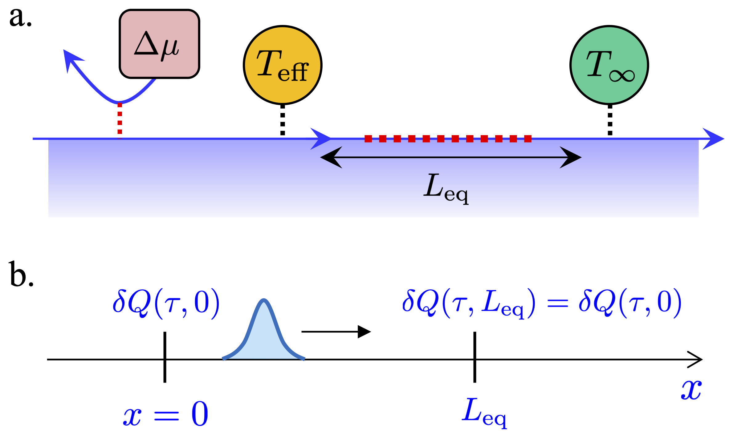
Figure 1: (a) A typical experimental setup for studying relaxation processes at QH edge state is schematically shown. A non-equilibrium state with the effective noise temperature $T_{\rm eff}$ is created by injecting a charge current, e.g., via a voltage biased QPC. The state is detected downstream the injection point by measuring the electron distribution function or the current noise power. It is typically assumed that the state reaches local equilibrium with the temperature $T_{\infty}$ after characteristic distances $L_{\rm eq}$. (b) These schematics illustrate the argument presented in the main text that the intuitive picture of the equilibration process at the edge is incorrect, since it contradicts the charges conservation requirement.

However, the assumption of full equilibration of a one-dimensional state at distances longer than the characteristic length $L_{\rm eq}$ leads to the following charge conservation paradox (see Fig. 1b). Assuming the state is equilibrium, the spectral density of current fluctuations $\delta j$ (noise power) at zero frequency satisfies the fluctuation-dissipation relation $S(0)=\int dt\langle\delta j(t)\delta(0)\rangle=G_{q}T_{\infty}$, where $T_{\infty}$ is the temperature of the final state, and $G_{q}=e^{2}/2\pi\hbar$ is the conductance quantum. On the other hand, the same quantity can be expressed in terms of the variance of the charge $\delta Q(\tau)=\int_{0}^{\tau}dt\delta j(t)$ transmitted through a given cross-section for the long time $\tau$. Formally, $S(0)$ is given by the limit of $\langle[\delta Q(\tau)]^{2}\rangle/\tau$ at $\tau\to\infty$. For the infinite time interval the fluctuation $\delta Q(\tau)$ does not depend on the cross-section, due to the charge conservation, and can be written as an integral of the incident current $\delta j_{\rm in}$ over time. Therefore, contrary to the above result, the zero frequency noise power must take value $S(0)=G_{q}T_{\rm eff}$, where $T_{\rm eff}$ is so defined effective temperature of the initial non-equilibrium state. However, $T_{\rm eff}\neq T_{\infty}$ in general (as, e.g., in the case of the current injection via a QPC, see the discussion below), therefore the assumption of full equilibration at any finite distances breaks.

At any finite distance $L$ only low energy excitations are protected by the charge conservation from the equilibration, while high energy states most likely equilibrate quite soon after the injection of the current. In this Letter we propose an effective way to account such equilibrium states in the overall equilibration process, based on the transmission line model Stäbler and Sukhorukov (2022), which is closely related to the Caldeira-Leggett model of dissipative quantum systems Caldeira and Leggett (1983). We present the unknown part of the system that is weakly coupled to the edge state and equilibrates it as a set of locally equilibrium reservoirs (see Fig. 2). Coupling to these reservoirs leads also to the dissipation and relaxation of edge states, confirmed experimentally Bocquillon et al. (2013). We conjecture, that the details of a particular equilibration mechanism do not affect the universality of the equilibration process under the constraint of the requirement of the charge and energy conservation. Taking advantage of the simplicity of our model, we derive the asymptotic behavior of the electron distribution function at long distances $L$ from the injection point and demonstrate that its deviation from the eventual equilibrium state scales as $1/\sqrt{L}$, i.e., the characteristic equilibration length is infinite. Throughout the paper, we set $|e|=\hbar=k_{B}=1$.

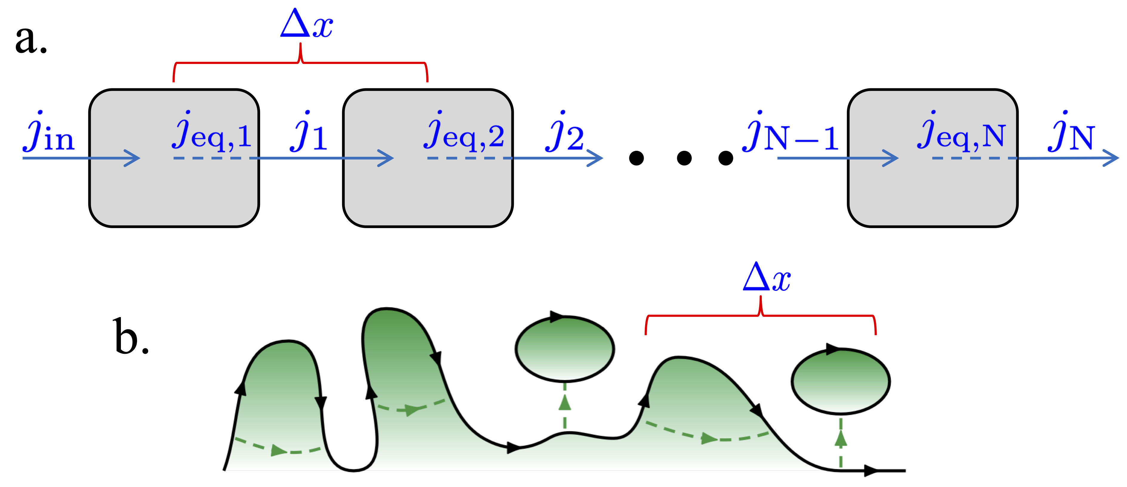
Figure 2: (a) The transmission line model of the QH edge at filling factor 1 is illustrated. The notations are explained in the main text. (b) A somewhat more realistic picture of a QH edge with disorder is shown. The edge state forms loops and puddles of the characteristic size $\Delta x$ connected by tunneling, shown by dashed lines.

Transmission line model. Following the Ref.  Stäbler and Sukhorukov (2022), we describe a QH edge at filling factor 1 with intrinsic dissipation with the help of the transmission line model, see Fig. 2. While propagating along the edge, the state sequentially enters and exist the metallic reservoirs, equally spaced at the distance $\Delta x$ and all having the same charge capacitance $C$ (The effects of randomness of this parameters, discussed in the end of the paper, is rather minor and can be neglected). We assume a long dwell time of electrons in the reservoirs, so that the state is fully equilibrated inside of them. The generally non-equilibrium current $j_{n-1}$ enters the $n$th reservoir, while the current that exits can be written as $j_{n}=G_{q}Q_{n}/C+j_{{\rm eq},n}$, where $j_{{\rm eq},n}$ is the equilibrium (with the temperature $T_{n}$) neutral fermionic current inside the reservoir. The assumption of the long dwell time implies also that currents $j_{n-1}$ and $j_{{\rm eq},n}$ are not correlated. The correlation between currents $j_{n-1}$ and $j_{n}$ arise via the charge continuity equation $dQ_{n}/dt=j_{n-1}-j_{n}$, which in frequency representation gives

$$j_{n}(\omega)=a(\omega)j_{n-1}+b(\omega)j_{{\rm eq},n},$$ (1)

where $a(\omega)=1/(1-i\omega\tau_{C})$ is the transmission amplitude, $b(\omega)=1-a(\omega)$, and $\tau_{C}=C/G_{q}$ is the charge relaxation time of the reservoirs. Applying this equation $N$ times, we obtain the edge state current $j_{N}$ at the distance $L=\Delta xN$ from the injection point (see Fig. 2a):

$$j_{N}(\omega)=a^{N}(\omega)j_{\rm in}(\omega)+b(\omega)\sum^{N}_{n=1}a^{N-n}(\omega)j_{{\rm eq},n}(\omega).$$ (2)

where $j_{\rm in}$ is the incident current.

In the weak coupling limit, where $\omega\tau_{C}$ is small, Eq. (2) can be used to derive the spectrum of the collective charge excitation. Considering the dynamics of the small excitation $\Delta j_{N}$, i.e., neglecting currents $j_{{\rm eq},n}$ in the Eq. (2), we write $\Delta j_{N}=a^{N}\Delta j_{\rm in}=e^{N\ln(a)}\Delta j_{\rm in}=e^{ikL}\Delta j_{\rm in}$, where $k$ is the wave vector of the excitation. Expanding $\ln(a)$ in small $\omega\tau_{C}$ and solving perturbatively for $\omega$, one finds the spectrum of the collective excitation:

$$\omega=(\Delta x/\tau_{C})k-i(\Delta x^{2}/2\tau_{C})k^{2}+\ldots,$$ (3)

where $k$ is the wave vector of excitation, the term $\Delta x/\tau_{C}$ is the group velocity, and the second term describes the dissipation and the decay of the collective mode . We are allowed to take the limit of $\Delta x\to 0$ by keeping the group velocity constant, assuming the capacitance $C$ scales linearly with $\Delta x$. However, the decay rate would vanish in this limit, while experimentally it has been shown to be finite . Thus, in the following discussion we assume $\Delta x$ to be finite and take the limit of small temperatures $T_{\rm eff}\tau_{C}\ll 1$.

Spectral density of current noise. Formally, the transmission line model can be viewed as the Langevin equation theory Slobodeniuk et al. (2013); Idrisov et al. (2017, 2022), where the incident current $j_{\rm in}$ and reservoir currents $j_{{\rm eq},n}$ are uncorrelated and considered as Langevin sources, or equivalently, as a scattering theory Sukhorukov (2016) following from the Hamiltonian approach Furusaki and Matveev (1995). Independently of the approach, the spectral density of the current fluctuations (noise power) defined as $S_{n}(\omega)=\int dte^{i\omega t}\langle\delta j_{n}(t)\delta j_{n}(0)\rangle$ immediately follows from the Eq. (2):

$$S_{N}(\omega)={\cal T}^{N}(\omega)S_{\rm in}(\omega)+{\cal R}(\omega)\sum_{n=1}^{N}{\cal T}^{N-n}(\omega)S_{{\rm eq},n}(\omega),$$ (4)

where $S_{\rm in}(\omega)$ is the noise power of the incident current, $S_{{\rm eq},n}(\omega)=G_{q}\omega/(1-e^{-\omega/T_{n}})$ is noise power of the locally equilibrium neutral currents of the reservoirs, and we introduced the transmission ${\cal T}(\omega)=|a(\omega)|^{2}=1/[1+(\omega\tau_{C})^{2}]$ and reflection ${\cal R}(\omega)=1-{\cal T}(\omega)$ coefficients for currents.

We are interested in the behavior of noise at long distances $N\gg 1$, and in the limit of small $\omega\tau_{C}\sim T_{\rm eff}\tau_{C}\ll 1$. Therefore, one can approximate ${\cal T}^{N}$ with the exponential function:

$${\cal T}^{N}(\omega)=e^{-N(\omega\tau_{C})^{2}},\quad N\gg 1.$$ (5)

In the limit $N\gg N_{0}=1/(\tau_{C}T_{\rm eff})^{2}\gg 1$ this exponential function cuts off the narrow frequency interval around zero frequency and thus sets a new energy scale $\Omega_{N}=1/(\sqrt{N}\tau_{C})\ll T_{\rm eff}$. The new length scale $L_{0}=\Delta xN_{0}$ is the characteristic length of the partial equilibration, as we show next. Before this distances the weak coupling to reservoirs can be treated perturbatively, and in general the result depends on details of the initial state in a non-universal way. Therefore, we focus on the limit of $L\gg L_{0}$, i.e., $N\gg N_{0}$ and resum the series in Eq. (4).

First we note, that at frequencies $\omega\gg\Omega_{N}$ the first term in Eq. (4) is exponentially small. The sum in the second term rapidly converges at the upper limit, assuming that $S_{{\rm eq},n}$ slowly converges towards the limit $S_{{\rm eq},\infty}$. Below we will show that this is indeed the case. Thus we can replace $S_{{\rm eq},n}$ with its value at $n=N$ and resum the series, which gives $S_{N}(\omega)=S_{{\rm eq},N}(\omega)$ for $\omega\gg\Omega_{N}$. At frequencies $\omega\sim\Omega_{N}\ll T_{\rm eff}$ the situation is more intricate. The first term in Eq. (4) takes a simple form $T_{\rm eff}G_{q}{\cal T}^{N}$. The sum in the second term can be presented as $G_{q}T_{N}(1-{\cal T}^{N})+G_{q}{\cal R}\sum_{n=1}^{N}{\cal T}^{N-n}(T_{n}-T_{N})$ after resuming the geometrical series. However, the second contribution in this term is sub-leading, if $S_{{\rm eq},n}$ slowly converges towards the limit $S_{{\rm eq},\infty}$, because the factor ${\cal R}$ scales as $1/N$ at $\omega\sim\Omega_{N}$. Finally, the noise power takes the form

$$S_{N}(\omega)=G_{q}(T_{\rm eff}-T_{N}){\cal T}^{N}(\omega)+S_{{\rm eq},N}(\omega)$$ (6)

where we have omitted sub-leading terms. Thus, the noise power acquires a sharp peak around zero frequencies that prevents the full relaxation of initial state to the equilibrium at finite distances. In particular, $S_{N}(0)=S_{\rm in}(0)$, which guarantees the charge conservation.

Energy balance. The temperature $T_{N}$ of the $N$th reservoir in Eq. (6) can be found from the energy balance equation $\Delta J_{N+1}=\Delta J_{N}$, where the energy current of a single channel, $\Delta J_{N}=(1/2G_{q})\langle j_{N}^{2}(t)\rangle=(1/4\pi G_{q})\int d\omega\Delta S_{N}$, is regularized by subtracting the eventual equilibrium contribution: $\Delta S_{N}\equiv S_{N}-S_{{\rm eq},\infty}$. By substituting $S_{N}$ from Eq. (6) in the energy balance equation, one obtains

$$\partial_{N}\int d\omega S_{{\rm eq},N}(\omega)=G_{q}(T_{\rm eff}-T_{\infty})\int d\omega{\cal R}{\cal T}^{N},$$ (7)

where we neglected sub-leading terms. Calculating the frequency integrals in this equation and integrating over $N$, we arrive at the following result:

$$T_{N}-T_{\infty}=-\frac{3}{2\pi^{3/2}\sqrt{N}}\frac{T_{\rm eff}-T_{\infty}}{\tau_{C}T_{\infty}}.$$ (8)

Therefore, indeed $T_{N}$ slowly converges to its limit $T_{\infty}$. Note also the presence of the small parameter $\tau_{C}T_{\infty}$ in the denominator of this expression. It agrees with the earlier made remark that this asymptotic behavior sets at $N\sim N_{0}=1/(\tau_{C}T_{\rm eff})^{2}\gg 1$, i.e., at distances $L\sim L_{0}=\Delta x/(\tau_{C}T_{\rm eff})^{2}$. This characteristic length scale agrees also with the relaxation length that follows directly from the spectrum of the collective charge mode (3).

Finally, the asymptotic value of the temperature $T_{\infty}$ can be found by comparing the heat flux quantum carried by the equilibrium edge state to the injected heat:

$$J_{q}=\frac{\pi T_{\infty}^{2}}{12}=(1/4\pi G_{q})\int d\omega(S_{\rm in}-S_{q}),$$ (9)

where we have subtracted the vacuum contribution $S_{q}=G_{q}\omega\theta(\omega)$. Two temperatures, $T_{\rm eff}$ and $T_{\infty}$, are generally different parameters of the noise power of the incident non-equilibrium current $j_{\rm in}$. However, often they are related to each other via the common energy scale. For instance, if the current source is created by injecting electrons into the edge state via a QPC at zero bath temperature, the noise power reads: $S_{\rm in}(\omega)=S_{\rm q}(\omega)+RD\left[\sum_{\pm}S_{\rm q}(\omega\pm\Delta\mu)-2S_{\rm q}(\omega)\right]$, where $D=1-R$ is the transmission probability of the QPC, and $\Delta\mu$ is voltage bias Blanter and Büttiker (2000). Thus, $S_{\rm in}(0)=G_{q}RD\Delta\mu$, and $T_{\rm eff}=RD\Delta\mu$. The integral on the right hand side of the Eq. (9) takes the value $(1/4\pi)RD\Delta\mu^{2}$, so that $T_{\infty}=\sqrt{(3/\pi^{2})RD}\Delta\mu$. Therefore, in this particular case two temperatures differ only by a numerical factor, and $T_{\infty}>T_{\rm eff}$.

Electron distribution function. According to the effective field theory of QH edge states Wen (1990) and the bosonization technique Giamarchi (2004) the electron distribution function is given by the expression

$$f_{N}(\varepsilon)\propto\int dte^{-i\varepsilon t}\langle e^{-i\phi_{N}(t)}e^{i\phi_{N}(0)}\rangle,$$ (10)

where $e^{i\phi_{N}}$ represents an electron operator in the channel exiting the $N$th reservoir, and the phase operator is related to the current as $j_{N}=-(1/2\pi)\partial_{t}\phi_{N}$. Assuming the current noise is Gaussian (the non-Gaussian effects are sub-leading in $1/N$ Levkivskyi and Sukhorukov (2012)), the average in this equation reads:

$$\ln\langle e^{-i\phi_{N}(t)}e^{i\phi_{N}(0)}\rangle=2\pi i\langle j_{\rm in}\rangle t\\ +\langle\phi_{N}(t)\phi_{N}(0)-\phi_{N}^{2}(t)/2-\phi_{N}^{2}(0)/2\rangle.$$ (11)

By substituting the Eq. (6) to this expression and then to Eq. (10), we observe that the leading order contribution to the noise power $S_{{\rm eq},N}$ simply returns the equilibrium fermionic distribution function $f_{{\rm eq},N}=1/[1+e^{(\varepsilon-\mu)/T_{N}}]$, where $\mu=2\pi\langle j_{\rm in}\rangle+\varepsilon_{F}$. By expanding this distribution function in small $T_{N}-T_{\infty}$ we find the leading order correction $(T_{N}-T_{\infty})\partial_{T_{\infty}}f_{{\rm eq},\infty}$ to the eventual equilibrium distribution $f_{{\rm eq},\infty}$. It scales downs as $1/\sqrt{N}$ according to the result (8).

Another leading order correction arises from the first term in Eq. (6). We note that it is not small only at frequencies or the order of $\Omega_{N}\ll T_{\rm eff}$, while the main contribution in the integral in Eq. (10) comes from the leading term $S_{{\rm eq},\infty}$ that sets the time scale $t\sim 1/T_{\rm eff}\ll 1/\Omega_{N}$. At this time scale the first term in the Eq. (6) can be considered as the delta function of frequency, which in the time domain gives the correction $G_{q}(T_{\rm eff}-T_{\infty})/2\sqrt{\pi N}\tau_{C}$ (replacing $T_{N}\to T_{\infty}$) to instant fluctuations of the current $\langle\delta j^{2}(0)\rangle$. Thus, the phase correlation function on the right hand side of the Eq. (11) acquires the correction $-2\pi^{2}t^{2}\langle\delta j^{2}(0)\rangle$. After expanding the average in the Eq. (10) with respect to this correction and evaluating the time convolution with the leading order equilibrium correlation function one obtains the correction $(\sqrt{\pi}/2\sqrt{N}\tau_{C})(T_{\rm eff}-T_{\infty})\partial^{2}_{\epsilon}f_{{\rm eq},\infty}$ to the equilibrium distribution $f_{{\rm eq},\infty}$, where we used $G_{q}=1/2\pi$. Putting these two corrections together, we obtain our main result:

$$f_{N}-f_{{\rm eq},\infty}=\frac{\sqrt{\pi}}{2}\frac{T_{\rm eff}-T_{\infty}}{\sqrt{N}\tau_{C}T_{\infty}^{2}}\cdot g(z),$$ (12)

$$g(z)=\partial^{2}_{z}f_{F}(z)+\frac{3z}{\pi^{2}}\partial_{z}f_{F}(z),\quad z=\frac{\varepsilon-\mu}{T_{\infty}},$$

where, we recall, $f_{F}(z)=1/(1+e^{z})$ and $\mu=2\pi\langle j_{\rm in}\rangle+\varepsilon_{F}$. We conclude that the correction to the final equilibrium distribution function scales down slowly as $1/\sqrt{N}$ and is universally expressed in terms of the “deformations” of the equilibrium distribution function and of the parameters $T_{\rm eff}$ and $T_{\infty}$ of the initail state. Thus, the characteristic equilibration length formally is absent. Nevertheless, the overall prefactor in Eq. (LABEL:Final_result) can be conveniently estimated as $\sqrt{L_{0}/L}\times(T_{\rm eff}-T_{\infty})/T_{\rm eff}$, where $L_{0}$ is the introduced earlier relaxation length of the collective charge excitation. We recall, that only at distances $L\gg L_{0}$ the correction to the final distribution function acquires its universal form (LABEL:Final_result).

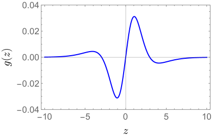
Figure 3: The dimensionless function $g(z)$ defined in the Eq. (LABEL:Final_result) is plotted versus the normalized energy $z=(\varepsilon-\mu)/T_{\infty}$.

Discussion. It remains to discuss several additional aspects of our theory. First of all, details of the particular kind of coupling of the edge state to reservoirs assumed in our model is likely not important. For instance, one can replace it with just a small capacitive coupling of the channel to otherwise isolated reservoirs. Then the transmission probability of the current generally behaves as ${\cal T}=1-\alpha\omega^{2}+\ldots$, where the constant $\alpha$ depends on the strength of capacitive coupling and is small. Thus in the limit of weak coupling ${\cal T}$ takes exactly same form as the one used in the paper, and in particular, the limit (5) still holds.

Next, if the disorder at the edge of a QH system is responsible for the relaxation process, then it is natural to assume that capacitances of the reservoirs or coupling constants fluctuate from one reservoir to another. Assuming that the parameter $\tau_{C,n}^{2}$ is random function with the average value $\tau_{C}^{2}$ and variance $\tau_{C}^{4}$, in Eq. (5) ${\cal T}^{N}$ has to be replaced with ${\cal P}_{N}=\prod_{n}{\cal T}_{n}=\exp[-\omega^{2}\sum_{n}\tau_{C,n}^{2}]$. We first account for the self-averaging effect: $\langle{\cal P_{N}}\rangle=\exp[-N(\omega\tau_{C})^{2}+(1/2)N(\omega\tau_{C})^{4}]$, where we averag over eventual Gaussian fluctuations of $\sum_{n}\tau_{C,n}^{2}$. Thus, we see that at relevant frequencies where $N(\omega\tau_{C})^{2}\sim 1$, the second term in the exponent scales as $1/N$ and gives a sub-leading contribution, that can be neglected. The variance of ${\cal P}_{N}$ can be easily calculated: $\langle\delta{\cal P}^{2}_{N}\rangle=2N(\omega\tau_{C})^{4}\langle{\cal P_{N}}\rangle^{2}\sim 1/N$. Therefore, the typical fluctuation correction to the initial condition contribution to $S_{N}$ in Eq. (6) at relevant frequencies $\omega\sim\Omega_{N}$ scales as $1/\sqrt{N}$ and can be neglected.

Finally, we note that our results can be easily generalized to arbitrary integer filling factors, including an experimentally important case of $\nu=2$. For example, in the latter case, the transmission line model applies separately to the dipole and charged mode, if tunneling between QH edge channels is negligible. However, if the injection and detection takes place in the same QH channel, one needs to account for the fact that for strong Coulomb interactions such channel has equal coupling to both modes. In this case the parameter $1/\tau_{C}$ in the result (LABEL:Final_result) splits in the sum of two contributions from the two modes divided by $4$.

To summarize, we addressed an experimentally relevant problem of the equilibration of chiral QH edge state. We started by presenting a simple physical argument that shows that the assumption of characteristic time scale for the equilibration breaks down, because it contradicts the charge conservation requirement. We used a transmission line model that effectively accounts for the dissipation and equilibration to find the spectral density of current noise. Then we applied the bosonization technique to evaluate corrections to the locally equilibrium electron distribution function. We showed that the the correction scales down slowly as $\sqrt{L_{0}/L}$ as a function of the distance $L$, where $L_{0}$ is the relaxation length of the charged mode.

We are grateful to Florian Stäbler for fruitful discussions. EVS acknowledges the financial support from the Swiss National Science Foundation.

References

- Bisognin et al. (2019) R. Bisognin, A. Marguerite, B. Roussel, M. Kumar, C. Cabart, C. Chapdelaine, A. Mohammad-Djafari, J.-M. Berroir, E. Bocquillon, B. Plaçais, et al., Nature Communications 10, 3379 (2019).
- Duprez et al. (2019) H. Duprez, E. Sivre, A. Anthore, A. Aassime, A. Cavanna, A. Ouerghi, U. Gennser, and F. Pierre, Phys. Rev. X 9, 021030 (2019).
- Bhattacharyya et al. (2019) R. Bhattacharyya, M. Banerjee, M. Heiblum, D. Mahalu, and V. Umansky, Phys. Rev. Lett. 122, 246801 (2019).
- Nakamura et al. (2020) J. Nakamura, S. Liang, G. C. Gardner, and M. J. Manfra, Nature Physics 16, 931 (2020).
- Jezouin et al. (2016) S. Jezouin, Z. Iftikhar, A. Anthore, F. D. Parmentier, U. Gennser, A. Cavanna, A. Ouerghi, I. P. Levkivskyi, E. Idrisov, E. V. Sukhorukov, et al., Nature 536, 58 (2016).
- Idrisov et al. (2017) E. G. Idrisov, I. P. Levkivskyi, and E. V. Sukhorukov, Phys. Rev. B 96, 155408 (2017).
- Slobodeniuk et al. (2013) A. O. Slobodeniuk, I. P. Levkivskyi, and E. V. Sukhorukov, Phys. Rev. B 88, 165307 (2013).
- Sivre et al. (2018) E. Sivre, A. Anthore, F. D. Parmentier, A. Cavanna, U. Gennser, A. Ouerghi, Y. Jin, and F. Pierre, Nature Physics 14, 145 (2018).
- Lin et al. (2021) C. Lin, M. Hashisaka, T. Akiho, K. Muraki, and T. Fujisawa, Nature Communications 12, 131 (2021).
- Sivre et al. (2019) E. Sivre, H. Duprez, A. Anthore, A. Aassime, F. D. Parmentier, A. Cavanna, A. Ouerghi, U. Gennser, and F. Pierre, Nature Communications 10, 5638 (2019).
- Altimiras et al. (2010a) C. Altimiras, H. le Sueur, U. Gennser, A. Cavanna, D. Mailly, and F. Pierre, Nature Physics 6, 34 (2010a).
- Kovrizhin and Chalker (2012) D. L. Kovrizhin and J. T. Chalker, Phys. Rev. Lett. 109, 106403 (2012).
- Levkivskyi and Sukhorukov (2012) I. P. Levkivskyi and E. V. Sukhorukov, Phys. Rev. B 85, 075309 (2012).
- Slobodeniuk et al. (2016) A. O. Slobodeniuk, E. G. Idrisov, and E. V. Sukhorukov, Phys. Rev. B 93, 035421 (2016).
- Itoh et al. (2018) K. Itoh, R. Nakazawa, T. Ota, M. Hashisaka, K. Muraki, and T. Fujisawa, Phys. Rev. Lett. 120, 197701 (2018).
- Lin et al. (2019) C. Lin, R. Eguchi, M. Hashisaka, T. Akiho, K. Muraki, and T. Fujisawa, Phys. Rev. B 99, 195304 (2019).
- Rodriguez et al. (2020) R. H. Rodriguez, F. D. Parmentier, D. Ferraro, P. Roulleau, U. Gennser, A. Cavanna, M. Sassetti, F. Portier, D. Mailly, and P. Roche, Nature Communications 11, 2426 (2020).
- Grenier et al. (2011) C. Grenier, R. Hervé, G. Fève, and P. Degiovanni, Modern Physics Letters B 25, 1053 (2011).
- Jullien et al. (2014) T. Jullien, P. Roulleau, B. Roche, A. Cavanna, Y. Jin, and D. C. Glattli, Nature 514, 603 (2014).
- Bäuerle et al. (2018) C. Bäuerle, D. C. Glattli, T. Meunier, F. Portier, P. Roche, P. Roulleau, S. Takada, and X. Waintal, Reports on Progress in Physics 81, 056503 (2018).
- Fletcher et al. (2019) J. D. Fletcher, N. Johnson, E. Locane, P. See, J. P. Griffiths, I. Farrer, D. A. Ritchie, P. W. Brouwer, V. Kashcheyevs, and M. Kataoka, Nature Communications 10, 5298 (2019).
- Altimiras et al. (2010b) C. Altimiras, H. le Sueur, U. Gennser, A. Cavanna, D. Mailly, and F. Pierre, Phys. Rev. Lett. 105, 226804 (2010b).
- le Sueur et al. (2010) H. le Sueur, C. Altimiras, U. Gennser, A. Cavanna, D. Mailly, and F. Pierre, Phys. Rev. Lett. 105, 056803 (2010).
- Tewari et al. (2016) S. Tewari, P. Roulleau, C. Grenier, F. Portier, A. Cavanna, U. Gennser, D. Mailly, and P. Roche, Phys. Rev. B 93, 035420 (2016).
- Imambekov et al. (2012) A. Imambekov, T. L. Schmidt, and L. I. Glazman, Rev. Mod. Phys. 84, 1253 (2012).
- Stäbler and Sukhorukov (2022) F. Stäbler and E. Sukhorukov, Phys. Rev. B 105, 235417 (2022).
- Caldeira and Leggett (1983) A. Caldeira and A. Leggett, Physica A: Statistical Mechanics and its Applications 121, 587 (1983).
- Bocquillon et al. (2013) E. Bocquillon, V. Freulon, J.-. M. Berroir, P. Degiovanni, B. Plaçais, A. Cavanna, Y. Jin, and G. Fève, Nature Communications 4, 1839 (2013).
- Idrisov et al. (2022) E. G. Idrisov, I. P. Levkivskyi, and E. V. Sukhorukov, Phys. Rev. B 106, L121405 (2022).
- Sukhorukov (2016) E. V. Sukhorukov, Physica E: Low-dimensional Systems and Nanostructures 77, 191 (2016).
- Furusaki and Matveev (1995) A. Furusaki and K. A. Matveev, Phys. Rev. B 52, 16676 (1995).
- Blanter and Büttiker (2000) Y. Blanter and M. Büttiker, Physics Reports 336, 1 (2000).
- Wen (1990) X. G. Wen, Phys. Rev. B 41, 12838 (1990).
- Giamarchi (2004) T. Giamarchi, Quantum Physics in One Dimension (Claverdon Press Oxford, 2004).