Patch-MI: Enhancing Model Inversion Attacks via Patch-Based Reconstruction

Abstract

Model inversion (MI) attacks aim to reveal sensitive information in training datasets by solely accessing model weights. Generative MI attacks, a prominent strand in this field, utilize auxiliary datasets to recreate target data attributes, restricting the images to remain photo-realistic, but their success often depends on the similarity between auxiliary and target datasets. If the distributions are dissimilar, existing MI attack attempts frequently fail, yielding unrealistic or target-unrelated results. In response to these challenges, we introduce a groundbreaking approach named Patch-MI, inspired by jigsaw puzzle assembly. To this end, we build upon a new probabilistic interpretation of MI attacks, employing a generative adversarial network (GAN)-like framework with a patch-based discriminator. This approach allows the synthesis of images that are similar to the target dataset distribution, even in cases of dissimilar auxiliary dataset distribution. Moreover, we artfully employ a random transformation block, a sophisticated maneuver that crafts generalized images, thus enhancing the efficacy of the target classifier. Our numerical and graphical findings demonstrate that Patch-MI surpasses existing generative MI methods in terms of accuracy, marking significant advancements while preserving comparable statistical dataset quality. For reproducibility of our results, we make our source code publicly available in https://github.com/jonggyujang0123/Patch-Attack.

I Introduction

The last decade has witnessed unparalleled advancements in deep learning technology, particularly driven by deep neural networks (DNNs). These advancements have not only broken records in diverse benchmarks but also unlocked a plethora of new services, such as AI chatbots, image generation, and intelligent assistants [1, 2, 3]. While these services herald unprecedented improvements in our daily lives, a potential risk remains: DNNs’ ability to retain sensitive information [4, 5]. This concern is spotlighted as many services frequently make DNN models publicly accessible through open-sourced APIs, like Pytorch/Tensorflow Hub, apparently in pursuit of public interest, but potentially leading to unforeseen privacy challenges.

Figure 1: Illustration of our motivation. Using an 8x8 patch-wise discriminator, the Patch-MI method successfully synthesizes target images (English alphabet) from the auxiliary dataset (Korean Hangeul), even though the auxiliary dataset is dissimilar to the Alphabet dataset.

The widespread belief that DNNs naturally protect sensitive training data has been sharply questioned by recent research, revealing a worrisome vulnerability to malicious use of publicly available DNN weights [6, 7, 8]. This vulnerability poses a threat to well-intentioned regulations like the EU’s General Data Protection Regulation (GDPR), which campaigns “the right to erasure/restriction of data processing” [9]. By focusing on model inversion (MI) attacks, a type of invasion aimed at retrieving sensitive information, we highlight a startling and urgent need to defend against breaches of regulatory protections [10, 11]. Should these attacks succeed, they could not only violate fundamental data protection principles but also cause serious financial and social damage, emphasizing the desperate need for strong defenses in our increasingly interconnected digital world.

In the initial phase of MI attacks, several pieces of research were towards tabular data classifiers, which are simpler than those for high-dimensional data such as images, text, and voices [10, 11, 12]. Subsequent studies [13, 14] focused on MI attack techniques with the aid of generative models to create photo-realistic images. While generative MI attack methods have demonstrated success in attacking private datasets, they face challenges, including the need for auxiliary data closely resembling the private dataset. More recently, an innovative approach utilizing random transformations to devise a more adaptable MI attack for private datasets is proposed [6], although the reliance on auxiliary datasets continues to present a formidable obstacle.

Contributions.

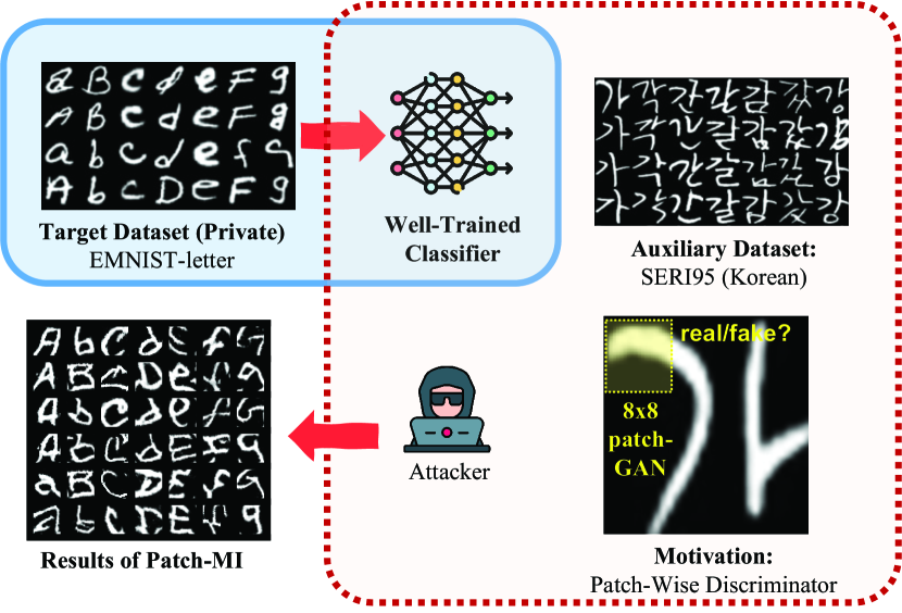
In this paper, we introduce an MI attack method that reconstructs characteristics of a private dataset by combining auxiliary image patches, as illustrated in Fig. 1. We postulate a publicly available classifier trained with a private dataset and demonstrate that our patch generative adversarial network (GAN)-inspired technique effectively rebuilds the training dataset despite dissimilar distribution with the auxiliary dataset. Utilizing a GAN-like approach with a patch-based discriminator, we enumerate the key contributions as follows:

1. We offer a novel probabilistic interpretation of the MI attack, subsequently formulating a loss function to minimize the Jensen-Shannon (JS) divergence between the private dataset and generated images. The loss function is equivalent to maximizing the mutual information between the generated images and the target label, thereby aligning with the InfoGAN [15] structure.

2. We employ a random transformation block to each generated image and subsequently forward it to the target classifier, with the aim of maximizing the target class logits.

3. We execute an MI attack on target DNNs, utilizing three distinct datasets, thereby illustrating that our method exhibits reduced reliance on auxiliary datasets, particularly within the context of shape-related handwriting datasets.

4. Our contribution extends to an end-to-end MI attack approach that does not require pre-trained generators.

II Related Works

Here, we provide an in-depth analysis of MI attacks, whose objective is to uncover the sensitive attributes embedded within private datasets through target DNNs, assuming that attackers have access to these models.

Optimization-based MI attack.

The concept of the MI attack was first delineated by [10] within the context of logistic regression. This seminal work demonstrated that an attacker, armed with partial information about the target DNN, could indeed extract sensitive information. Building upon this foundation, subsequent studies [11, 12] formulated more generalized MI attack algorithms. By employing gradient descent, these enhanced approaches aimed to unveil sensitive information embedded within target models. However, such MI attacks are less effective against intricate and deep multi-layer neural networks. This limitation arises from the fact that data trained in the target classifier often occupy only a small portion of the image space, as elucidated in [16]. A recent study introduces an MI attack technique that eschews the use of generative models for binary classifiers; yet, the challenge concerning photo-realistic images persists [17].

Generative MI attack.

To rectify the limitations of optimization-based MI attacks, recent innovations have adopted generative models such as GANs [18] and VAEs [19] to guarantee the photorealism of resultant images. In this context, the authors of [20] skillfully employed a GAN pre-trained on public data for MI attacks, utilizing blurred or masked faces as supplementary information. Early influential works revealed that optimizing latent vectors to maximize posterior probability within target classifiers could expose sensitive traits of private datasets while maintaining photorealistic quality [21, 13, 22]. This marked a shift towards a generative MI paradigm, finely tuning latent space to minimize the target classifier’s cross-entropy. Furthermore, the authors of [23] enhanced this approach by integrating soft labels from the target classifier, representing a significant advance in the development of refined and effective attack strategies.

Extensions of generative MI attack.

In an effort to reconstruct the target class distribution, the authors of [7] pioneered a variational MI attack to ascertain the mean and variance of latent vectors, utilizing a deep flow model for accurate approximation. Subsequent contributions in [6, 24, 25, 26] provided a robust enhancement through image transformation, reinforcement learning, and label-guidance. Additionally, the authors of [14] investigated GAN-based MI attacks against ensemble classifiers, thereby evidencing enhanced dependability in the attack methodology.

Remaining Challenges.

Prevailing research frequently depends on the unfeasible supposition that the image prior corresponds with the target prior in the training of generative models, a misalignment potentially leading to inaccuracies. This paper contests this traditional notion by suggesting mitigation of this assumption, positing uniformity among the priors for various image segments. Our investigation focuses on enhancing MI attacks on DNN classifiers, especially in instances where the auxiliary and target datasets have dissimilar distributions.

III Patch Model Inversion Attack

In this section, we begin with an introduction to the threat scenario that forms the foundation of our MI attack method. We then present a novel probabilistic interpretation of MI attacks and frame an optimization problem targeting the minimization of the JS divergence between the attacker’s distribution and the target data distribution. Our findings show that this optimization problem can be reformulated into the form of InfoGAN [15]. Furthermore, our utilization of a patch-wise discriminator negates the conventional assumption of identical distribution between target and auxiliary datasets. This enhances the practicality and effectiveness of our method in real-world MI scenarios, where such an assumption may not necessarily be valid.

Threat scenario.

Let’s consider a scenario where a programmer has trained a DNN classifier using a private dataset, denoted as $\mathcal{D}_{\text{tar}}$, and subsequently uploaded the model weights to a public platform such as Tensorflow/Pytorch Hub. The target dataset is a general image dataset for classification tasks, meaning that it comprises image instances $\mathbf{x}\in\mathbb{R}^{w\times h}$ and corresponding label instances $y\in\{0,...,C-1\}$, where $C$ represents the number of classes within the dataset. The attacker’s objective is to uncover the sensitive characteristics inherent to the target classifier, the weights of which are readily accessible to the public. Additionally, it is presumed that the attacker is capable of inferring the rough dataset type by examining the model’s description, examples of which might include categories such as gray-scale handwriting and color natural images.

III-A Patch-MI: A New Probabilistic Interpretation

The principal objective of the MI attack is to uncover the sensitive characteristics of the target dataset. In pursuit of this aim, our approach endeavors to approximate the distribution of the target dataset $p_{\textrm{tar}}(\mathbf{x}|y)$ through the utilization of a generative model denoted by $q(\mathbf{x})$ for given target label $y$. To articulate the approximation of the target posterior distribution within the target classifier, we employ the following notation:

$$\hat{p}_{\textrm{tar}}(y|\mathbf{x}):\mathbb{R}^{w\times h}\rightarrow\Delta^{C},$$ (1)

where $w$ and $h$ represent the width and height of the input images, respectively, while $\Delta^{C}$ is the $C$-dimensional probability simplex.

Assumption 1 (Well-trained classifier).

We proceed under the assumption that the target classifier is a robust and well-behaved classifier, capable of successfully categorizing the majority of the training data, i.e. $\hat{p}_{\text{tar}}(y|\mathbf{x})\approx p_{\text{tar}}(y|\mathbf{x})$ for all $(\mathbf{x},y)\in\mathcal{D}_{\text{tar}}$.

By presenting Assumption 1, we can represent the target dataset-related distributions by target classifier $\hat{p}_{\text{tar}}$ instead of true dataset $p_{\text{tar}}$.

Goal.

We present an optimization problem that aims to minimize the JS divergence between the target data distribution $\hat{p}_{\textrm{tar}}(\mathbf{x}|y)$ and the MI attacker $q(\mathbf{x})$, a kind of generative model. This approach seeks to closely mimic the approximated target data distribution:

$$\arg\min_{q\sim Q_{\mathbf{x}}}D_{\text{JS}}\left(q(\mathbf{x})\|\hat{p}_{\mathrm{tar}}(\mathbf{x}|y)\right),$$ (2)

where $Q_{\mathbf{x}}$ denotes a set of possible probability distribution functions on a space $\mathbb{R}^{w\times h}$.

Furthermore, to achieve success in the MI attack, it is essential to utilize an auxiliary dataset encapsulating partial information akin to that of the target dataset, denoted by the distribution $p_{\textrm{aux}}(\mathbf{x})$. As it is infeasible to sample or acquire the approximated distribution $\hat{p}_{\text{tar}}(\mathbf{x}|y)$, our objective translates to obtaining and minimizing an upper bound of the problem articulated in (2). This objective requires us to introduce the following assumption.

Assumption 2 (Sampling probability inequality).

For an MI attacker $q(\mathbf{x})$ corresponding to the target class $y\in\{0,1,...,C-1\}$, the following inequality holds: $1=q(y|\mathbf{x})\geq p_{\text{tar}}(y|\mathbf{x})$. Similarly, $1=p_{\mathrm{tar}}(y|\mathbf{x})$ holds if $\mathbf{x}\sim p_{\mathrm{tar}}(\mathbf{x}|y)$.

Theorem 1.

Under Assumption 2, the following inequality holds:

$$\begin{split}&D_{\mathrm{JS}}\left(q(\mathbf{x})\|\hat{p}_{\mathrm{tar}}(\mathbf{x}|y)\right)\\ \leq&D_{\mathrm{JS}}\big{(}q(\mathbf{x})\|\hat{p}_{\mathrm{tar}}(\mathbf{x})\big{)}-\frac{1}{2}\mathbb{E}_{q(\mathbf{x})}\left[\log\left(\hat{p}_{\mathrm{tar}}(y|\mathbf{x})\right)\right].\end{split}$$ (3)

Proof:

The proof is shown in Appendix A. ∎

Theorem 1 delineates the upper bound of our objective function, conforming to Assumption 2. Here, we reformulate the MI optimization problem as

$$\arg\min_{q\sim Q_{\mathbf{x}}}D_{\text{JS}}(q(\mathbf{x})\|\hat{p}_{\mathrm{tar}}(\mathbf{x}))-\lambda\mathbb{E}_{q(\mathbf{x})}[\log(\hat{p}_{\mathrm{tar}}(y|\mathbf{\mathbf{x}}))],$$ (4)

where a weight $\lambda\geq 1/2$ is added to the attacker loss to control the posterior probability. As discussed in [7], the power posterior [28] let us control the effect of posterior probability in bayes prior, i.e. $q^{*}_{\lambda}(\mathbf{x})\propto p_{\text{aux}}(\mathbf{x})\hat{p}_{\text{tar}}^{\lambda}(y|\mathbf{x})$.

Figure 2: Illustration of the Patch-MI attack method. For the generator, we simply reuse the standard DCGAN structure for image generation. For the patch-wise discriminator, we commence by applying a Conv2d layer, utilizing a filter whose size corresponds to the patch size and a stride size determined by the subtraction of overlapped pixels from the patch size. Subsequently, 1x1 convolution layers calculate $D_{i}$. Furthermore, the generated images are subjected to random transformation before being forwarded to the target classifier. By consolidating all results and minimizing the MI attack loss, we successfully facilitate the MI attack.

Patch-MI loss function.

At the beginning of this section, we assume that the attacker can access an auxiliary dataset that helps the attacker to generate photo-realistic images. Now, in the equation (4), we can change the JS divergence term into a GAN objective function by defining a discriminator $\sigma(D(\mathbf{x}))=\frac{\hat{p}_{\mathrm{tar}}(\mathbf{x})}{\hat{p}_{\mathrm{tar}}(\mathbf{x})+q(\mathbf{x})}$, where $\sigma(a)=1/(1+\exp(-a))$, i.e. $D(\mathbf{x})=\log\frac{\hat{p}_{\mathrm{tar}}(\mathbf{x})}{q(\mathbf{x})}$. In addition, we define a generator $G(\mathbf{z})$ representing $q(\mathbf{x})$. We note that $q(\mathbf{x})$ can be sampled by $G(\mathbf{z})$, $\mathbf{z}\sim\mathcal{N}(\mathbf{0},\mathbf{I})$. Then, the MI attack problem can be formulated to generate images that 1) imitate the target dataset distribution and 2) maximize the target posterior probability, as follows:

$$\arg\min_{G}\max_{D}\underset{\mathbf{x}\sim p_{\mathrm{tar}}}{\mathbb{E}}\left[\log\sigma(D(\mathbf{x}))\right]+$$ (5)

$$\mathbb{E}_{\mathbf{z}}\left[\log\big{(}1-\sigma(D(G(\mathbf{z}))\big{)}-\lambda\log\hat{p}_{\mathrm{tar}}(y|G(\mathbf{z}))\right].$$

As in previous studies [13, 21, 7], our next step is to approximate the distribution of the target dataset into the auxiliary dataset. However, instead of the distribution of the whole image, we assume that the distributions of image patches from the target and auxiliary datasets are identical. The following assumption enables us to design our patch-based MI attack.

Assumption 3 (Partially similar auxiliary dataset).

Let us consider a sequence of overlapped patches $x_{1},\ldots,x_{N}$ of an image $\mathbf{x}$ and the adjacent pixels of the $i$-th patch $x_{-i}$. It is assumed that the patches are conditionally independent, which means that $\prod_{i=1}^{N}p_{\mathrm{tar}}(x_{i}|x_{-i})=p_{\mathrm{tar}}(\mathbf{x})$. The distribution of the auxiliary dataset and the target dataset for the overlapped patches are approximately the same; that is, $p_{\mathrm{tar}}(x_{i}|x_{-i})\approx p_{\mathrm{aux}}(x_{i}|x_{-i})$.

Under Assumption 3, by defining the discriminator for the $i$-th patch of an image $\mathbf{x}$ as $D_{i}$ the optimization of the discriminator can be decomposed to per-patch discriminators, as follows:

$$D(\mathbf{x})=\log\frac{\hat{p}_{\mathrm{tar}}(\mathbf{x})}{q(\mathbf{x})}=\sum_{i=1}^{N}\log\frac{\hat{p}_{\mathrm{tar}}(x_{i}|x_{-i})}{q(x_{i}|x_{-i})}=\sum_{i=1}^{N}D_{i}(\mathbf{x}).$$ (6)

Then, the Patch-MI loss function can be rewritten as

$$\begin{split}&\arg\min_{G}\max_{D}\mathbb{E}_{\mathbf{x}\sim p_{\mathrm{aux}}}\left[\log\sigma\left(\sum_{i=1}^{N}D_{i}(\mathbf{x})\right)\right]\\ &~{}~{}~{}~{}+\mathbb{E}_{\mathbf{z}}\Bigg{[}\log\left(1-\sigma\left(\sum_{i=1}^{N}D_{i}(G(\mathbf{z}))\right)\right)\\ &~{}~{}~{}~{}~{}~{}~{}~{}~{}~{}~{}~{}~{}~{}~{}~{}~{}~{}-\lambda\log\hat{p}_{\mathrm{tar}}(y|G(\mathbf{z}))\Bigg{]}.\end{split}$$ (7)

Proposition 1.

As similar to InfoGAN paper [15], the mutual information between the target classes $y$ and the generative images $G(\mathbf{z})$ is bounded by

$$\begin{split}&I(y;G(\mathbf{z}))=H(y)-H(y|G(\mathbf{z}))\\ &=H(y)+\mathbb{E}_{\mathbf{x}\sim G(\mathbf{z})}\left[\mathbb{E}_{y\sim q(y|\mathbf{x})}[\log q(y|\mathbf{x})]\right]\\ &=D_{\mathrm{KL}}\big{(}q(y|\mathbf{x})\|\hat{p}_{\mathrm{tar}}(y|\mathbf{x})\big{)}\\ &~{}~{}~{}~{}+H(y)+\mathbb{E}_{\mathbf{x}\sim G(\mathbf{z})}\left[\log\hat{p}_{\text{tar}}(y|\mathbf{x})\right]\\ &\geq\mathbb{E}_{\mathbf{x}\sim G(\mathbf{z})}\left[\log\hat{p}_{\text{tar}}(y|\mathbf{x})\right].\end{split}$$ (8)

Then, by using the result of Proposition 1, our objective function is to learn generator $G(\mathbf{z})$ that imitates the auxiliary data distribution $p_{\mathrm{aux}}(x_{i}|x_{-i})$. While training, another objective is to maximize the mutual information between the target class $y$ and the generated images $G(\mathbf{z})$. In other words, our method is analogous to replacing the categorical latent vector in InfoGAN with the target classifier.

III-B Patch Discriminator with Overlapped Patches

In Fig. 2, the schematic representation of the Patch-MI approach is depicted. The generator $G(\cdot)$ employs the standard DCGAN architecture [29], utilizing transposed convolution layers to create images from the random vector $\mathbf{z}\sim\mathcal{N}(\mathbf{0},\mathbf{I})$. Contrary to earlier studies, our discriminator differentiates fake patches from realistic ones, rather than the entire image. In a manner akin to ViTGAN [30], patches are overlapped to ensure photorealism, followed by embedding into a fixed-length vector using the Conv2d layer. Subsequently, the discriminators’ outputs $D_{i}$ are obtained via $1\times 1$ convolution.

(a) Patch-MI with patch size of 8 and stride of 4. ($\lambda=0$)

(b) Canonical GAN.

Figure 3: Examples of the generated images of our method and canonical GAN. Both generative models are trained with the MNIST dataset, i.e., handwritten digits from 0 to 9. Within our approach, the patch and stride sizes of the discriminator are set at 8 and 4, respectively, given an image size of 32. As evident from the figure, our technique is capable of creating images that are not contained within the MNIST dataset.

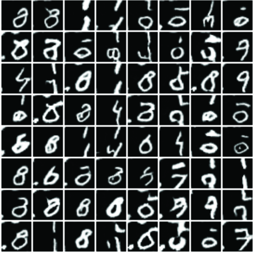
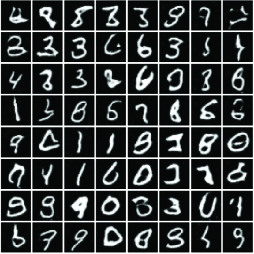
Figure 3 showcases images generated by both standard GAN and our approach with $\lambda=0$ for comparison. Notably, both methodologies are trained on the MNIST dataset, with our method displaying greater flexibility in image generation compared to the traditional GAN.

III-C Data Augmentation on Synthetic Images

In [6], a data selection algorithm is to devise a more general MI attack. Under this approach, images undergo random transformations or augmentations, with selections being made based on the highest average confidence level over diverse transformations. A parallel intuition is evident in [14], where the incorporation of additional ensemble models is demonstrated to boost the efficacy of the MI attacker. Mirroring these approaches, we utilize data augmentation to enable the generator $G$ to acquire more accurate images. Let us define the image augmentation function as $T$, which can be Resize, RandomCrop, RandomRotation, and the like. Subsequently, we task the image generator $G$ with maximizing $\log\hat{p}_{\text{tar}}(T\circ G(\mathbf{z}))$ instead of $\log\hat{p}_{\text{tar}}(G(\mathbf{z}))$, as shown in Fig. 2.

III-D Relation to Existing Works

Baseline MI attack (BMI).

In the early stage of the MI attack studies, baseline MI (BMI) attacks [10, 11] are proposed approaches to find an optimal instance that maximizes the target posterior probability as follows:

$$\mathbf{x}^{*}=\arg\max_{\mathbf{x}\in\mathbb{R}^{w\times h}}\hat{p}_{\text{tar}}(y|\mathbf{x}).$$ (9)

In the BMI approach, the reconstructed images are founded by applying gradient descent, i.e., $\frac{\partial p_{\text{tar}}(y|\mathbf{x})}{\partial\mathbf{x}}$. Note that this method is a case of our method with $\lambda=\infty$, where the photo-realism is neglected. As we will show in Section IV, the images generated with this objective function are not natural images.

Generative MI attack (GMI).

In generative MI (GMI) attack approaches the aim is to find an optimal latent vector $\mathbf{z}^{*}$ that maximizes the probability $\hat{p}_{\mathrm{tar}}(y|G(\mathbf{z}))$ for a given class $y$ [13, 21]. That is, the objective function can be written as

$$\mathbf{z}^{*}=\arg\max_{\mathbf{z}}\lambda\log\hat{p}_{\mathrm{tar}}(y|(G(\mathbf{z}))+\log(\sigma(D(G(\mathbf{z})))).$$ (10)

While akin to our method (7), the GMI differs in that it 1) necessitates a pre-trained generative model $G$ with an auxiliary dataset for one-time whole image generation, and 2) learns a sample $\mathbf{z}$ without replicating the private dataset’s distribution. Conversely, our generator $G$ simulates the private dataset’s distribution $p_{\mathrm{tar}}(\mathbf{x}|y)$ for each class in a singular training, unlike the GMI approach, which demands re-training per sample.

Variational MI attack (VMI).

In the variational MI (VMI) attack [7], a variational inference-based objective function is used to avoid collapsing the output images. Their objective function is derived from the KL divergence between the target/attacker data distribution:

$$q^{*}(\mathbf{z})=\arg\min_{q\in Q_{\mathbf{z}}}\left\{\mathbb{E}_{\mathbf{z}\sim q}\left[D_{\mathrm{KL}}(q(\mathbf{z})\|\hat{p}_{\mathrm{tar}}(\mathbf{z}))-\log\hat{p}_{\mathrm{tar}}(\mathbf{z})\right]\right\}$$ (11)

They use StyleGAN2 [31] and normalizing flows [32] for better disentanglement. The VMI attack can mimic the distribution of the target dataset from the target classifier with variational inference; however, their pre-trained generator is still constrained by the auxiliary dataset. That is, the VMI cannot generate an image that cannot be generated via the pre-trained generative model.

IV Main Experimental Results

(a) Experiment 1. The target dataset is MNIST, and the auxiliary dataset is SERI95.

(b) Experiment 2. The target dataset is EMNIST-letter, and the auxiliary dataset is SERI95.

Figure 4: Depiction of the target dataset and auxiliary dataset for two distinct experiments. In (4(a)), the target dataset is designated as MNIST, and the auxiliary dataset is identified as SERI95. Analogously, the target dataset in (4(b)) is EMNIST-letter. In the second experiment, the focus is directed at the first 10 classes from a total of 26 classes.

In this section, we evaluate the proposed MI attack (Patch-MI) and show its superiority by comparing it to existing MI attacks.

IV-A Experimental Details

Hardware.

Our experiments are conducted at a workstation with 12th Gen Intel(R) Core(TM) i9-12900K 16-Core Processor CPU @ 5.20GHz and one NVIDIA Geforce RTX 3090 GPU.

Experimental scenario.

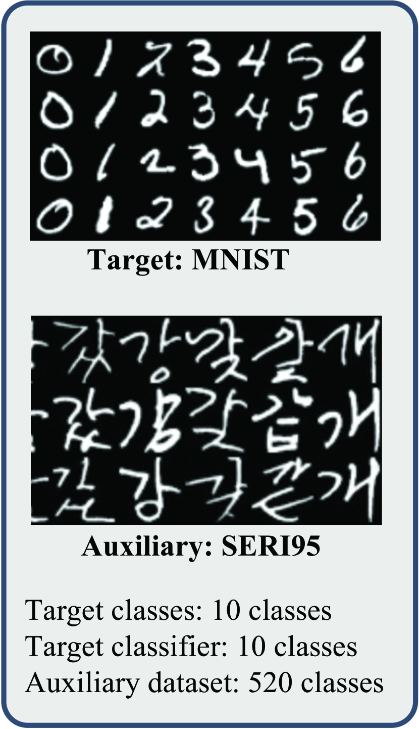
In our experiments, we employ three experiments of the following (target, auxiliary) dataset pairs to evaluate MI attack methods on the cross-domain dataset scenarios:

1. MNIST [33] and SERI95 [34]

2. EMNIST-letter [35] and SERI95

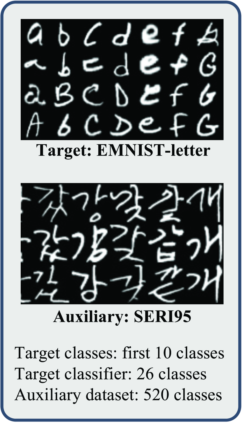
For the MNIST and EMNIST-letter datasets, our objective centers on the reconstruction of image shapes within the target datasets, leading us to select a letter dataset that excludes digits and alphabets. We cordially introduce SERI95, which encompasses 520 of the most commonly used Hanguel characters, each represented by approximately 1000 samples each. The design of the experiments is illustrated in Fig. 4.

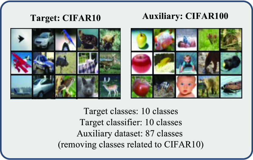
Aside from this, we conduct additional experimental results for the CIFAR10 experiment, where we exclude images in the CIFAR100 dataset that bear labels corresponding to the CIFAR10 dataset. For the additional experiments, please refer Section V.

Baseline methods.

In our benchmarking, we compare our methodology with 1) BMI [10], 2) GMI [13], and 3) VMI [7], each employing a common generator trained with DCGAN [29]. Contemporary literature has manifested a prevailing trend focused on executing MI attacks at elevated resolutions [14, 6, 24]. Within these methodologies, auxiliary datasets used are those that either share classes with the target dataset or possess a structural resemblance. In contrast, our objective is to explore the manner in which the target and auxiliary datasets symbolize essentially disparate subjects. Specifically, this paper orchestrates experiments in an unprecedented scenario wherein the distribution between the auxiliary and target datasets diverges markedly. In line with this, as foundational references for these investigations, we engage in comparative analysis with the elemental methodologies in low-resolution, namely BMI, GMI, and VMI.

Evaluation metrics.

For our evaluation, we train an evaluation classifier models with deeper layers, in which other configurations are set the same with the target classifier with different random seeds. Then, we assess the top-1 accuracy (Acc@1), top-5 accuracy (Acc@5), and confidence level pertaining to the target class, employing the evaluation classifier models. Subsequently, we leverage the Fréchet Inception Distance (FID) score [36], a well-known metric for measuring generated image qualities. This score means the distance between the feature vectors of images from the target dataset and the generated dataset, where extraction is performed using an Inception-v3 model [37] tuned on ImageNet [38]. The FID score corresponding to a heightened similarity between the two datasets; however, per-class evaluation metric is still required. Thus, we utilize metrics such as improved precision and recall [39], in conjunction with density and coverage [40] on an individual label, to assess the diversity of the images, by following [6].

IV-B Target Classifiers

We trained ResNet-18 model [41] for the target classifier and DLA-34 model [42] for the evaluation classifier. We note that the target classifiers have top-1 accuracy of 99.44% for MNIST and 95.60% for EMNIST-letter. Also, the evaluation classifiers have top-1 accuracy of 99.58% for MNIST and 95.30% for EMNIST-letter.

MNIST.

We trained ResNet-18 as target classifier and DLA-34 as evaluation classifier. Both models are trained using the stochastic gradient descent (SGD) optimizer, with the initial learning rate of $2.5\cdot 10^{-2}$, momentum of 0.9, and weight decay of $5.0\cdot 10^{-4}$. The images are normalized with $\mu=\sigma=0.5$. The batch size is 256. The models are trained for 20 epochs. The learning rate is reduced by a factor of 0.1 at 10-th, 15-th, and 18-th epochs. After training, the validation accuracy is 99.44% on target classifier and 99.58% on evaluation classifier, respectively.

EMNIST-letter.

Similar to the MNIST dataset, we trained ResNet-18 and DLA-34 models as target and evaluation classifiers, respectively. All the setups are same except for maximum epochs of 30. Also, the learning rate is reduced by a factor of 0.1 at 15-th, 22-nd, and 27-th epochs. After training is done, the validation accuracy is 95.60% and 95.30%, respectively.

IV-C MI Attacker

For the image generator and discriminator, we employ canonical DCGAN [29] model, except for the modification in discriminator on Fig. 2. where the patch size and stride size are 8 and 4, respectively. In the target posterior term in the loss function (7), we use $\lambda=30$.

Hyper-parameter setup and model settings.

DCGAN model in [29]. For patch embedding, we use Conv2d network with a patch size of 8, stride size of 4, and padding size of 0. We use Adam optimizer [43] in our method, where the learning rate is fixed at $1.0\cdot 10^{-3}$. We trained 30 epochs for the target attacker.

Generator and discriminator.

For generator, we follow the standard DCGAN model [29]. That is, the latent vector $\mathbf{z}$ is forwarded into three consecutive transposed convolution layers with kernel size of 4, stride size of 2, and padding size of 1, in which rectified linear unit (ReLU) activation is applied except for the last layer. In the discriminator, the Conv2d layer first embeds the image patches into vectors, with patch size of 8, stride size of 4, and padding size of 0. Then, three 1x1 convolution layers are placed after the embedding convolution layer for distinguish real patches from fake patches.

Output augmentation.

In our method, the generated images $G(\mathbf{z})$ is randomly transformed before forwarding to the target classifier. For experiments 1 and 2, the image transformer consists of 1) random rotation of [-20, 20] degrees, 2) random resized crop of 32x32 images with scales [0.85, 1.0] and ratio [0.9, 1.1]. Let us define the transform function as $T$. Then, the classifier output is defined by

$$\frac{1}{2}\left(\hat{p}_{\text{tar}}(y|\mathbf{x})+\hat{p}_{\text{tar}}(y|T(\mathbf{x}))\right).$$ (12)

GAN label smoothing.

In our experiments, basic GAN loss function often diverges; hence, we add one-sided label smooth by reducing the true label from 1.0 to 0.6. This assumes 60% of the auxiliary patch are false; thus, the generator does not longer need to learn all the auxiliary patch. In our experiments adding a label smoothing trick helps convergence. We also check that employing LS-GAN [44] can also helps enhancing training stability.

TABLE I: Evaluation results for our MI method on MNIST and EMNIST datasets, where the auxiliary dataset is SERI95.

Dataset Methods Acc@1 $\uparrow$ Acc@5 $\uparrow$ Confidence ↑ Precision ↑ Recall ↑ Coverage ↑ Density ↑ FID ↓ MNIST BMI [10] 47.54% 91.67% 45.74% 0.0000 0.0000 0.0000 0.0000 407.7958 GMI [13] 75.72% 99.13% 67.74% 0.0115 0.0956 0.0051 0.0016 155.1654 VMI[7] 94.25% 99.64% 89.27% 0.0000 0.0379 0.0000 0.0000 204.4829 Patch-MI (ours) 99.72% 100.00% 98.13% 0.0028 0.1199 0.0016 0.0026 160.0833 EMNIST BMI[10] 18.09% 74.36% 18.35% 0.0000 0.0000 0.0000 0.0000 426.1645 GMI [13] 54.20% 91.53% 46.75% 0.0095 0.0339 0.0051 0.0035 140.8377 VMI[7] 90.95% 98.99% 83.86% 0.0005 0.0166 0.0002 0.0004 161.0970 Patch-MI (ours) 99.68% 100.00% 97.08% 0.0044 0.0328 0.0024 0.0012 152.5619 *Best: bold and underline, second-best: underline.

IV-D Comparison with Existing MI Attacks

In the empirical examination presented in Table I, numerical evaluation metrics were employed to assess two distinct sets of simulations and four methodologies. The results within Table I demonstrate that the proposed method outperforms the alternatives in both MNIST and EMNIST across accuracy-related metrics (Acc@1, Acc@5, and Confidence). This superiority is principally attributed to the effect of generalization induced through random transformations and patch-based MI techniques.

Further analysis reveals an encouraging performance by the proposed method in metrics pertaining to the quality aspect of the dataset, placing it favorably when contrasted with conventional methods. While the GMI approach is found to be comparable, it simultaneously lowers accuracy considerably by generating target-unrelated samples, albeit gaining advantage in the FID, Precision, and coverage domains. Despite this, the proposed method manifests a notable persistence in maintaining a comparable statistical quality of the dataset in terms of quality, without incurring substantial degradation in accuracy. This underscores the robustness and efficacy of the proposed approach in a multifaceted evaluative context.

TABLE II: Ablation study on our method with and without Patch-wise discriminator and random transformation, on EMNIST-letter dataset.

Patch size Trans. Acc@1 $\uparrow$ Acc@5 $\uparrow$ Confidence ↑ Precision ↑ Recall ↑ Coverage ↑ Density ↑ FID ↓ 32 (full) ✗ 69.82% 95.42% 59.56% 0.0000 0.0009 0.0000 0.0000 229.5503 32 (full) ✓ 90.69% 99.71% 83.67% 0.0003 0.0377 0.0002 0.0003 202.6455 8 ✗ 91.33% 99.67% 81.81% 0.0027 0.0366 0.0015 0.0010 171.1700 8 ✓ 99.68% 100.00% 97.08% 0.0044 0.0328 0.0024 0.0012 152.5619 *Best: bold and underline.

IV-E Ablation Study

In order to establish the proposed method, we utilized patch-wise discriminator and random transformations. To ascertain the effects of these two additional features, we conducted an ablation study in Table II. We note that the Patch-MI attack, without the inclusion of two features, is identical to the method described in [14]. First, when neither of the two features is applied, that is, a full-size GAN without random transformation, the performance is slightly better than GMI but inferior to VMI. However, with the addition of transformation, it is possible to achieve a performance comparable to VMI, and by altering the patch size to 8, a slightly elevated performance in comparison to VMI can be realized. By employing both features, as previously mentioned, the ability to outperform existing fundamental MI techniques can be achieved. This study underscores the nuanced interplay of these options in enhancing the overall efficacy of the proposed method.

(a) MNIST dataset.

(b) EMNIST dataset.

Figure 5: Visualization of the randomly chosen outputs for various MI attack methods on the MNIST dataset.

IV-F Graphical Results

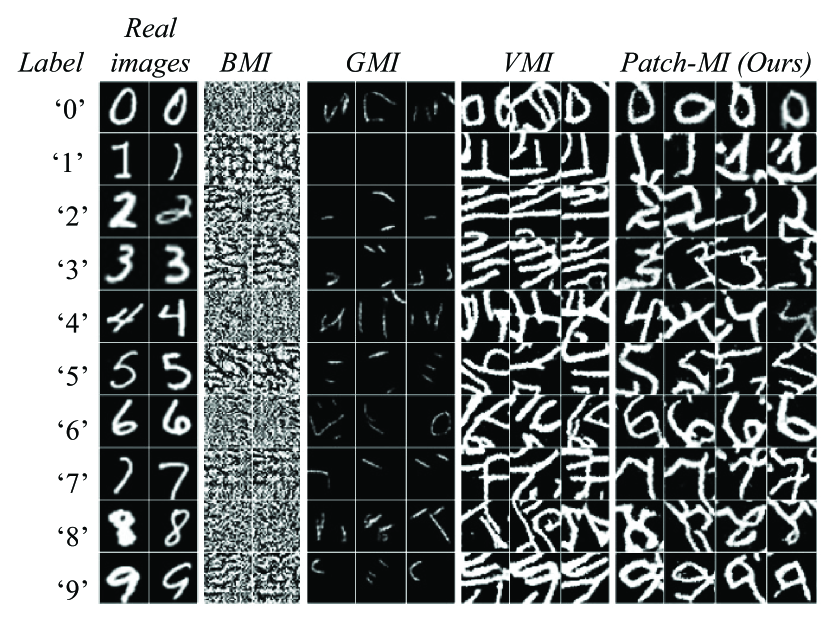
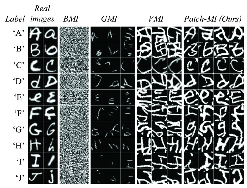
In Fig. 5, the subfigures (5(a)) and (5(b)) depict the visualizations of various MI methods applied to the MNIST and EMNIST-letter datasets. Overall, BMI tends to generate noisy images, and both GMI and VMI exhibit a decrease in structural similarity, which can be observed as a limitation due to their inability to learn at the patch level. In contrast, the proposed method is observed to produce images with structural similarity, even when attacking an EMNIST-letter and MNIST classifiers using Korean Hanguel data. This finding underlines the capability of the proposed approach to maintain structural coherence across diverse contexts, highlighting its potential efficacy and robustness.

V Additional Experiment: CIFAR10

In addition to experiments with black and white images targeting the MNIST and EMNIST datasets, we have conducted supplementary experiments on color images with the CIFAR10 dataset as the target. Detailed experimental setups and results will be discussed in the remainder of this section.

V-A Experiment Setup

Target and evaluation classifiers.

We trained ResNet-18 as the target classifier and DLA-34 as the evaluation classifier. Both models are trained using the stochastic gradient descent (SGD) optimizer, with an initial learning rate of 2.5e-2, momentum of 0.9, and weight decay of 5.0e-4. The images are normalized with $\mu=\sigma=0.5$. The batch size is 256. The models are trained for 20 epochs. The learning rate is reduced by a factor of 0.1 at 10, 15, and 18 epochs. After training, the validation accuracy is 99.44% on the target classifier and 99.58% on the evaluation classifier, respectively.

Figure 6: Depiction of the target dataset and auxiliary dataset in the experiment 3. The target dataset is designated as CIFAR10, and the auxiliary dataset is identified as CIFAR100. Unfortunately, there are some overlapped labeled data such as (bus, pickup truck, street car, tractor, lawn mower, rocket, dolphin, whale, ray, train, shark, aquarium fish, and leopard) in the CIFAR100 dataset, we remove them in our experiments.

Dataset.

For the CIFAR100 dataset, the images with labels (bus, pickup truck, street car, tractor, lawn mower, rocket, dolphin, whale, ray, train, shark, aquarium fish, and leopard) related with the CIFAR10 dataset is removed in our experiment.

Created Image Augmentation.

In our method, the generated images $\mathbf{x}=G(\mathbf{z})$ is randomly transformed before forwarding to the target classifier. For experiments 1 and 2, the image transformer consists of 1) padding 4 pixels, 2) random rotation of [-45, 45] degrees, and 3) random horizontal flip. Let us define the transform function as $T^{\prime}$. Then, the classifier output is defined by

$$\frac{1}{2}\left(\hat{p}_{\text{tar}}(y|\mathbf{x})+\hat{p}_{\text{tar}}(y|T^{\prime}(\mathbf{x}))\right).$$ (13)

V-B Experimental Results

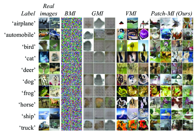
In Tables III and IV, we evaluate various MI attack methods based on metrics encompassing the entire dataset (Table III) and per-class metrics (Table IV). Similarly to the gray-scale dataset (MNIST and EMNIST-letter), the Patch-MI outperforms all other MI techniques in terms of accuracy. In contrast, the VMI exhibits better performance than our proposed approach concerning the FID score. However, in the per-class results, VMI and Patch-MI were found to have similar performance. That is, in the per-class statistics, VMI and Patch-MI have similar characteristics. The graphical results in Fig. 7 show the reason why the Patch-MI has a lower FID than the VMI: the Patch-MI creates images similar to the target label by slightly sacrificing photo-realism, whereas VMI generates more diverse images that are distant from the target image but classified with lower confidence levels to the corresponding label.

Hence, it was observed that Patch-MI has a lower FID score than VMI due to the diversity of output images. Conversely, when viewed on a per-class basis, the statistical quality is similar between VMI and Patch-MI, and in terms of accuracy, Patch-MI overwhelms other methods.

TABLE III: Evaluation results for our MI method on CIFAR10 datasets. Here, the dataset-wise metrics are written.

Acc@1 $\uparrow$ Acc@5 $\uparrow$ Confidence ↑ FID ↓ BMI 14.01% 56.61% 13.10% 427.8511 GMI 12.36% 66.18% 12.91% 211.9117 VMI 83.14% 99.11% 76.73% 48.4994 Patch-MI (ours) 96.47% 99.86% 91.66% 93.7527 *Best: bold and underline, second-best: underline.

TABLE IV: Evaluation results for our MI method on CIFAR10 dataset. In this table, the per-class-based metrics are indicated.

Precision ↑ Recall ↑ Coverage ↑ Density ↑ BMI 0.0000 0.0000 0.0000 0.0000 GMI 0.0795 0.0024 0.0717 0.0211 VMI 0.2085 0.0789 0.4690 0.2638 Patch-MI (ours) 0.2543 0.0483 0.5190 0.1912 *Best: bold and underline, second-best: underline.

Figure 7: Visualization of the generated images via various MI attack methods on the CIFAR10 dataset.

Further analysis with various attacker weights $\lambda$.

To address the conflicting metrics with accuracy: precision, recall, coverage, and density (PRCD), we conducted an experiment involving various values of attacker weight for the CIFAR 10 dataset. The numerical results are presented in Table V.

As indicated in the table, our proposed method outperforms the VMI scheme, albeit with a slight sacrifice in attack accuracy. However, the accuracy of our method remains higher than that of VMI. More significantly, our method excels in precision, recall, and coverage metrics, and is comparable in terms of density. This demonstrates that our method is superior to VMI in aspects other than FID, which is a density-based metric. Our analysis suggests that precision, recall, coverage, and density (PRCD) provide a more accurate assessment than FID.

• Tradeoff: The table illustrates a fundamental tradeoff between quality-related metrics (PRCD) and accuracy-related metrics (Acc@1, confidence). While our method exhibits superior performance in PRCD, there is a noticeable balance between these metrics and the traditional accuracy-related metrics. This tradeoff highlights the complexity of optimizing for multiple metrics in machine learning models and underscores the necessity of considering a diverse range of evaluation criteria to comprehensively assess model performance.

TABLE V: Evaluation results of the proposed method and VMI, where the experiments are conducted to verify the tradeoff between the accuracy and other data statistical metrics (PRCD).

Acc@1 $\uparrow$ Acc@5 $\uparrow$ Conf. ↑ FID ↓ Prec. ↑ Rec. ↑ Cov. ↑ Dens. ↑ PMI ($\lambda=50$) 96.47% 99.86% 91.66% 93.7527 0.2543 0.0483 0.5190 0.1912 PMI ($\lambda=10$) 92.89% 99.66% 86.82% 85.0515 0.2512 0.0928 0.5086 0.2153 PMI ($\lambda=5$) 89.01% 99.46% 82.78% 71.1711 0.2540 0.0963 0.5216 0.2370 PMI ($\lambda=2$) 81.54% 97.24% 76.44% 67.9040 0.2674 0.1037 0.5450 0.2224 VMI ($w=10^{-1}$) 78.66% 99.06% 72.65% 55.1312 0.2426 0.0895 0.4720 0.2192 VMI ($w=10^{-3}$) 83.14% 99.11% 76.73% 48.4994 0.2085 0.0789 0.4690 0.2638 VMI ($w=10^{-7}$) 83.99% 99.12% 76.45% 49.6053 0.2175 0.0565 0.5018 0.2546 VMI ($w=10^{-13}$) 65.37% 89.04% 60.59% 97.1975 0.1743 0.0533 0.3827 0.1916

Different target classifiers.

In the previous results, we have experimented with a target classifier. Here, we execute our method to attack various classifiers: ResNeXt29, VGG11, VGG19, and MobileNet v2 with the CIFAR 10 dataset, where all the classifiers are well-trained with many epochs. In Table VI, we denote the accuracy, confidence level, and FID score of the image obtained via PMI attack. As shown in the table, the proposed method consistently has high accuracy and high confidence in all the classifiers, while performing FID scores less than 100.0. These results note that our method can work generally on various target classifiers.

TABLE VI: Experimental results of PMI attacker for various classifiers: ResNeXt29[45], VGG11[46], VGG19, and MobileNet v2[47]. We note that the classifiers are well-trained with the CIFAR 10 dataset.

Acc@1 $\uparrow$ Acc@5 $\uparrow$ Confidence ↑ FID ↓ ResNet18 96.47% 99.86% 91.66% 93.7527 ResNeXt29 (32x4d) 93.70% 99.80% 88.68% 72.1683 VGG11 93.81% 99.75% 88.99% 94.8382 VGG19 99.09% 99.99% 95.43% 98.0052 MobileNet V2 99.28% 99.99% 96.19% 95.1164

VI Discussion

Limitations.

In this work, we have advanced the field of Patch-MI attacks, acknowledging existing constraints. Our methodology relies on assumptions regarding access to related auxiliary datasets and employs GANs, a choice that may not smoothly translate across all types of data. While effective in a white-box setting, extending this approach to gray-box or black-box scenarios presents intriguing avenues for future research. Additionally, we have demonstrated that the proposed method can attack the shape of low-resolution images under the framework of shape-related feature extraction, using only data that is dissimilar in shape. The generation of high-resolution images would be more computationally expensive, and the proposed method would likely need to incorporate several other appealing aspects.

Conclusion and further directions.

In summary, this paper unveils a cutting-edge MI attack technique that harnesses the local partial features of an auxiliary dataset to craft synthetic images targeting specific classifiers. The innovation lies in deploying a patch-based discriminator, which leads to more accurate, photo-realistic images that echo the characteristics of targeted classes. Demonstrated across diverse datasets, this methodology outperforms conventional MI attacks, signifying a leap toward securing deep learning models. However, its reliance on specialized auxiliary datasets and its potential struggles with complex or abstract classes reveal room for improvement. Future research may dwell on enhancing image synthesis for intricate categories or investigating alternative discriminators, opening doors to greater realism and versatility.

Appendix A Proof of Theorem 1

Theorem 1.

Under Assumption 2, the following inequality holds:

$$D_{\mathrm{JS}}\left(q(\mathbf{x})\|\hat{p}_{\mathrm{tar}}(\mathbf{x}|y)\right)$$ (14)

$$~{}~{}~{}~{}\leq D_{\mathrm{JS}}\big{(}q(\mathbf{x})\|\hat{p}_{\mathrm{tar}}(\mathbf{x})\big{)}-\frac{1}{2}\mathbb{E}_{q(\mathbf{x})}\left[\log\left(\hat{p}_{\text{tar}}(y|\mathbf{x})\right)\right].$$

To prove the Theorem, we have the following two Lemmas. For the proofs of the Lemmas, please see Appendices A-A and A-B.

Lemma 1.

By presuming Assumption 2, if $\mathbf{x}\sim q(\mathbf{x})$, the following inequality is satisfied:

$$\log\left(\frac{2q(\mathbf{x})}{q(\mathbf{x})+\hat{p}_{\mathrm{tar}}(\mathbf{x}|y)}\right)$$ (15)

$$~{}~{}~{}~{}~{}~{}\leq\log\left(\frac{2q(\mathbf{x})}{q(\mathbf{x})+\hat{p}_{\mathrm{tar}}(\mathbf{x})}\right)-\frac{1}{2}\log\hat{p}_{\mathrm{tar}}(y|\mathbf{x}).$$

Lemma 2.

Postulating Assumption 2, if $\mathbf{x}\sim\hat{p}_{\mathrm{tar}}(\mathbf{x}|y)$, the following equality holds:

$$\log\left(\frac{2\hat{p}_{\mathrm{tar}}(\mathbf{x}|y)}{q(\mathbf{x})+\hat{p}_{\mathrm{tar}}(\mathbf{x}|y)}\right)=\log\left(\frac{2\hat{p}_{\mathrm{tar}}(\mathbf{x})}{q(\mathbf{x})+\hat{p}_{\mathrm{tar}}(\mathbf{x})}\right).$$ (16)

Then, the following series of equations prove the theorem.

$$D_{\mathrm{JS}}\left(q(\mathbf{x})\|\hat{p}_{\mathrm{tar}}(\mathbf{x}|y)\right)$$

$$=\frac{1}{2}D_{\mathrm{KL}}\left(q(\mathbf{x})\|\frac{q(\mathbf{x})+\hat{p}_{\mathrm{tar}}(\mathbf{x}|y)}{2}\right)$$

$$~{}~{}~{}~{}+\frac{1}{2}D_{\mathrm{KL}}\left(\hat{p}_{\mathrm{tar}}(\mathbf{x}|y)\|\frac{q(\mathbf{x})+\hat{p}_{\mathrm{tar}}(\mathbf{x}|y)}{2}\right)$$

$$=\frac{1}{2}\mathbb{E}_{q(\mathbf{x})}\left[\log\left(\frac{2q(\mathbf{x})}{q(\mathbf{x})+\hat{p}_{\mathrm{tar}}(\mathbf{x}|y))}\right)\right]$$

$$~{}~{}~{}~{}+\frac{1}{2}\mathbb{E}_{\hat{p}_{\mathrm{tar}}(\mathbf{x}|y)}\left[\log\left(\frac{2\hat{p}_{\mathrm{tar}}(\mathbf{x}|y)}{q(\mathbf{x})+\hat{p}_{\mathrm{tar}}(\mathbf{x}|y)}\right)\right]$$ (17)

$$\overset{(a)}{\leq}\frac{1}{2}\mathbb{E}_{q(\mathbf{x})}\left[\log\left(\frac{2q(\mathbf{x})}{q(\mathbf{x})+\hat{p}_{\mathrm{tar}}(\mathbf{x})}\right)\right]$$

$$~{}~{}~{}~{}~{}+\frac{1}{2}\mathbb{E}_{\hat{p}_{\mathrm{tar}}(\mathbf{x})}\left[\log\left(\frac{2\hat{p}_{\mathrm{tar}}(\mathbf{x})}{q(\mathbf{x})+\hat{p}_{\mathrm{tar}}(\mathbf{x})}\right)\right]$$

$$~{}~{}~{}~{}~{}-\frac{1}{2}\mathbb{E}_{q(\mathbf{x})}\left[\log\left(\hat{p}_{\mathrm{tar}}(y|\mathbf{x})\right)\right]$$

$$=D_{\mathrm{JS}}\big{(}q(\mathbf{x})\|\hat{p}_{\mathrm{tar}}(\mathbf{x})\big{)}-\frac{1}{2}\mathbb{E}_{q(\mathbf{x})}\left[\log\left(\hat{p}_{\text{tar}}(y|\mathbf{x})\right)\right]$$

where inequality (a) holds since Lemmas 1 and 2 are true.

A-A Proof of Lemma 1

In Assumption 2, we have $1=q(y|\mathbf{x})\geq\hat{p}_{\mathrm{tar}}(y|\mathbf{x})$ if $\mathbf{x}\sim q(\mathbf{x})$ for the target class $y$. Also, since the target label is fixed as $y$ in an attack attempt, we let the target label probability as $p(c)$ is 1 if $c=y$ and 0 otherwise. Then, the following inequality holds:

$$\log\left(\frac{2q(\mathbf{x})}{q(\mathbf{x})+\hat{p}_{\mathrm{tar}}(\mathbf{x}|y)}\right)$$

$$=\log\left(\frac{2q(\mathbf{x})}{q(\mathbf{x})+\hat{p}_{\mathrm{tar}}(\mathbf{x})\hat{p}_{\mathrm{tar}}(y|\mathbf{x})}\right)$$

$$=\log\left(\frac{2q(\mathbf{x})}{q(\mathbf{x})+\hat{p}_{\mathrm{tar}}(\mathbf{x})}\right)$$ (18)

$$~{}~{}~{}~{}~{}~{}+\log\left(\frac{q(\mathbf{x})+\hat{p}_{\mathrm{tar}}(\mathbf{x})}{q(\mathbf{x})+\hat{p}_{\mathrm{tar}}(\mathbf{x})\hat{p}_{\mathrm{tar}}(y|\mathbf{x})}\right)$$

$$\leq\log\left(\frac{2q(\mathbf{x})}{q(\mathbf{x})+\hat{p}_{\mathrm{tar}}(\mathbf{x})}\right)-\log\hat{p}_{\mathrm{tar}}(y|\mathbf{x}).$$

A-B Proof of Lemma 2

Similar to the proof in Appendix A-A, if $\mathbf{x}\sim\hat{p}_{\mathrm{tar}}(y|\mathbf{x})$ for the target class $y$ and $1=\hat{p}_{\mathrm{tar}}(y|\mathbf{x})$, the following sequence of equalities show that Lemma 2 is true:

$$\log\left(\frac{2\hat{p}_{\mathrm{tar}}(\mathbf{x}|y)}{q(\mathbf{x})+\hat{p}_{\mathrm{tar}}(\mathbf{x}|y)}\right)$$

$$=\log\left(\frac{2\hat{p}_{\mathrm{tar}}(\mathbf{x})\hat{p}_{\mathrm{tar}}(y|\mathbf{x})}{q(\mathbf{x})+\hat{p}_{\mathrm{tar}}(\mathbf{x})\hat{p}_{\mathrm{tar}}(y|\mathbf{x})}\right)$$ (19)

$$=\log\left(\frac{2\hat{p}_{\mathrm{tar}}(\mathbf{x})}{q(\mathbf{x})+\hat{p}_{\mathrm{tar}}(\mathbf{x})}\right).$$

References

- [1] OpenAI, “Gpt-4 technical report,” 2023.
- [2] J. Oppenlaender, “The creativity of text-to-image generation,” in Proceedings of International Academic Mindtrek Conference. ACM, nov 2022. [Online]. Available: https://doi.org/10.1145%2F3569219.3569352
- [3] A. Ramesh, P. Dhariwal, A. Nichol, C. Chu, and M. Chen, “Hierarchical text-conditional image generation with clip latents,” 2022.
- [4] C. Song, T. Ristenpart, and V. Shmatikov, “Machine learning models that remember too much,” in Proceedings of ACM SIGSAC Conference on Computer and Communications Security, Oct. 2017, pp. 587–601.
- [5] V. Feldman and C. Zhang, “What neural networks memorize and why: Discovering the long tail via influence estimation,” in Proceedings of Advances in Neural Information Processing Systems, 2020.
- [6] L. Struppek, D. Hintersdorf, A. De Almeida Correira, A. Adler, and K. Kersting, “Plug & play attacks: Towards robust and flexible model inversion attacks,” in Proceedings of International Conference on Machine Learning, 2022, pp. 20 522–20 545.
- [7] K.-C. Wang, Y. Fu, K. Li, A. Khisti, R. Zemel, and A. Makhzani, “Variational model inversion attacks,” Proceedings of Advances in Neural Information Processing Systems, vol. 34, pp. 9706–9719, 2021.
- [8] N.-B. Nguyen, K. Chandrasegaran, M. Abdollahzadeh, and N.-M. Cheung, “Re-thinking model inversion attacks against deep neural networks,” in Proceedings of IEEE/CVF Conference on Computer Vision and Pattern Recognition, 2023, pp. 16 384–16 393.
- [9] EU, “General data protection regulation,” 2018. [Online]. Available: https://gdpr-info.eu/
- [10] M. Fredrikson, E. Lantz, S. Jha, S. Lin, D. Page, and T. Ristenpart, “Privacy in pharmacogenetics: An end-to-end case study of personalized warfarin dosing,” in Proceedings of USENIX Conference on Security Symposium, 2014, p. 17–32.
- [11] M. Fredrikson, S. Jha, and T. Ristenpart, “Model inversion attacks that exploit confidence information and basic countermeasures,” in Proceedings of ACM SIGSAC Conference on Computer and Communications Security, 2015, p. 1322–1333.
- [12] S. Hidano, T. Murakami, S. Katsumata, S. Kiyomoto, and G. Hanaoka, “Model inversion attacks for prediction systems: Without knowledge of non-sensitive attributes,” in Proceedings of Annual Conference on Privacy, Security and Trust, 2017, pp. 115–11 509.
- [13] Z. Yang, J. Zhang, E.-C. Chang, and Z. Liang, “Neural network inversion in adversarial setting via background knowledge alignment,” in Proceedings of ACM SIGSAC Conference on Computer and Communications Security, 2019, p. 225–240.
- [14] Q. Wang and D. Kurz, “Reconstructing training data from diverse ml models by ensemble inversion,” in Proceedings of IEEE/CVF Winter Conference on Applications of Computer Vision, 2022, pp. 2909–2917.
- [15] X. Chen, Y. Duan, R. Houthooft, J. Schulman, I. Sutskever, and P. Abbeel, “InfoGAN: Interpretable representation learning by information maximizing generative adversarial nets,” Proceedings of Advances in Neural Information Processing Systems, vol. 29, 2016.
- [16] C. Szegedy, W. Liu, Y. Jia, P. Sermanet, S. Reed, D. Anguelov, D. Erhan, V. Vanhoucke, and A. Rabinovich, “Going deeper with convolutions,” in Proceedings of IEEE/CVF Conference on Computer Vision and Pattern Recognition, 2015, pp. 1–9.
- [17] N. Haim, G. Vardi, G. Yehudai, O. Shamir, and M. Irani, “Reconstructing training data from trained neural networks,” in Proceedings of Advances in Neural Information Processing Systems, 2022, pp. 22 911–22 924.
- [18] I. Goodfellow, J. Pouget-Abadie, M. Mirza, B. Xu, D. Warde-Farley, S. Ozair, A. Courville, and Y. Bengio, “Generative adversarial networks,” Communications of the ACM, vol. 63, no. 11, pp. 139–144, 2020.
- [19] D. P. Kingma, M. Welling et al., “An introduction to variational autoencoders,” Foundations and Trends in Machine Learning, vol. 12, no. 4, pp. 307–392, 2019.
- [20] Y. Zhang, R. Jia, H. Pei, W. Wang, B. Li, and D. Song, “The secret revealer: Generative model-inversion attacks against deep neural networks,” in Proceedings of IEEE/CVF Conference on Computer Vision and Pattern Recognition, 2020, pp. 253–261.
- [21] Z. Yang, E.-C. Chang, and Z. Liang, “Adversarial neural network inversion via auxiliary knowledge alignment,” arXiv preprint arXiv:1902.08552, 2019.
- [22] M. Khosravy, K. Nakamura, N. Nitta, and N. Babaguchi, “Deep face recognizer privacy attack: Model inversion initialization by a deep generative adversarial data space discriminator,” in Proceedings of Asia-Pacific Signal and Information Processing Association Annual Summit and Conference, 2020, pp. 1400–1405.
- [23] S. Chen, M. Kahla, R. Jia, and G.-J. Qi, “Knowledge-enriched distributional model inversion attacks,” in Proceedings of the IEEE/CVF International Conference on Computer Vision, 2021, pp. 16 178–16 187.
- [24] G. Han, J. Choi, H. Lee, and J. Kim, “Reinforcement learning-based black-box model inversion attacks,” in Proceedings of IEEE/CVF Conference on Computer Vision and Pattern Recognition, 2023, pp. 20 504–20 513.
- [25] X. Yuan, K. Chen, J. Zhang, W. Zhang, N. Yu, and Y. Zhang, “Pseudo label-guided model inversion attack via conditional generative adversarial network,” Proceedings of Annual AAAI Conference on Artificial Intelligence, 2023.
- [26] H. Takahashi, J. Liu, and Y. Liu, “Breaching fedmd: Image recovery via paired-logits inversion attack,” in Proceedings of IEEE/CVF Conference on Computer Vision and Pattern Recognition, 2023, pp. 12 198–12 207.
- [27] F. Huszár, “How (not) to train your generative model: Scheduled sampling, likelihood, adversary?” 2015.
- [28] J. Knoblauch, J. Jewson, and T. Damoulas, “Generalized variational inference: Three arguments for deriving new posteriors,” 2019.
- [29] A. Radford, L. Metz, and S. Chintala, “Unsupervised representation learning with deep convolutional generative adversarial networks,” arXiv preprint arXiv:1511.06434, 2015.
- [30] K. Lee, H. Chang, L. Jiang, H. Zhang, Z. Tu, and C. Liu, “Vitgan: Training gans with vision transformers,” 2021.
- [31] T. Karras, S. Laine, M. Aittala, J. Hellsten, J. Lehtinen, and T. Aila, “Analyzing and improving the image quality of StyleGAN,” in Proc. CVPR, 2020.
- [32] D. Rezende and S. Mohamed, “Variational inference with normalizing flows,” in Proceedings of International Conference on Machine Learning, 2015, pp. 1530–1538.
- [33] Y. LeCun, C. Cortes, and C. Burges, “Mnist handwritten digit database,” ATT Labs [Online]. Available: http://yann.lecun.com/exdb/mnist, vol. 2, 2010.
- [34] G.-R. Park, I.-J. Kim, and C.-L. Liu, “An evaluation of statistical methods in handwritten hangul recognition,” International Journal on Document Analysis and Recognition, vol. 16, pp. 273–283, 2013.
- [35] G. Cohen, S. Afshar, J. Tapson, and A. van Schaik, “Emnist: an extension of mnist to handwritten letters,” 2017.
- [36] M. Heusel, H. Ramsauer, T. Unterthiner, B. Nessler, and S. Hochreiter, “Gans trained by a two time-scale update rule converge to a local nash equilibrium,” Proceedings of Advances in Neural Information Processing Systems, vol. 30, 2017.
- [37] X. Xia, C. Xu, and B. Nan, “Inception-v3 for flower classification,” in Proceedings of IEEE International Conference on Image, Vision and Computing, 2017, pp. 783–787.
- [38] J. Deng, W. Dong, R. Socher, L.-J. Li, K. Li, and L. Fei-Fei, “ImageNet: A large-scale hierarchical image database,” in Proceedings of IEEE/CVF Conference on Computer Vision and Pattern Recognition, 2009, pp. 248–255.
- [39] T. Kynkäänniemi, T. Karras, S. Laine, J. Lehtinen, and T. Aila, “Improved precision and recall metric for assessing generative models,” Proceedings of Advances in Neural Information Processing Systems, vol. 32, 2019.
- [40] M. F. Naeem, S. J. Oh, Y. Uh, Y. Choi, and J. Yoo, “Reliable fidelity and diversity metrics for generative models,” in Proceedings of International Conference on Machine Learning. PMLR, 2020, pp. 7176–7185.
- [41] K. He, X. Zhang, S. Ren, and J. Sun, “Deep residual learning for image recognition,” in Proceedings of IEEE/CVF Conference on Computer Vision and Pattern Recognition, 2016, pp. 770–778.
- [42] F. Yu, D. Wang, E. Shelhamer, and T. Darrell, “Deep layer aggregation,” in Proceedings of IEEE/CVF Conference on Computer Vision and Pattern Recognition, 2018, pp. 2403–2412.
- [43] D. P. Kingma and J. Ba, “Adam: A method for stochastic optimization,” arXiv preprint arXiv:1412.6980, 2014.
- [44] X. Mao, Q. Li, H. Xie, R. Y. Lau, Z. Wang, and S. Paul Smolley, “Least squares generative adversarial networks,” in Proceedings of IEEE International Conference on Computer Vision, 2017, pp. 2794–2802.
- [45] S. Xie, R. Girshick, P. Dollár, Z. Tu, and K. He, “Aggregated residual transformations for deep neural networks,” 2017.
- [46] K. Simonyan and A. Zisserman, “Very deep convolutional networks for large-scale image recognition,” 2015.
- [47] M. Sandler, A. Howard, M. Zhu, A. Zhmoginov, and L.-C. Chen, “Mobilenetv2: Inverted residuals and linear bottlenecks,” 2019.