Diff-OP3D: Bridging 2D Diffusion for Open Pose 3D Zero-Shot Classification

Abstract

With the explosive 3D data growth, the urgency of utilizing zero-shot learning to facilitate data labeling becomes evident. Recently, the methods via transferring Contrastive Language-Image Pre-training (CLIP) to 3D vision have made great progress in the 3D zero-shot classification task. However, these methods primarily focus on aligned pose 3D objects (ap-3os), overlooking the recognition of 3D objects with open poses (op-3os) typically encountered in real-world scenarios, such as an overturned chair or a lying teddy bear. To this end, we propose a more challenging benchmark for 3D open-pose zero-shot classification. Echoing our benchmark, we design a concise angle-refinement mechanism that automatically optimizes one ideal pose as well as classifies these op-3os. Furthermore, we make a first attempt to bridge 2D pre-trained diffusion model as a classifer to 3D zero-shot classification without any additional training. Such 2D diffusion to 3D objects proves vital in improving zero-shot classification for both ap-3os and op-3os. Our model notably improves by 3.5% and 15.8% on ModelNet10^‡ and McGill^‡ open pose benchmarks, respectively, and surpasses the current state-of-the-art by 6.8% on the aligned pose ModelNet10, affirming diffusion’s efficacy in 3D zero-shot tasks. Code will be available publicly at https://github.com/weiguangzhao/Diff-OP3D.

Figure 1: 3D Zero-shot Classification for Aligned Poses and Open Poses. (a) is a 3D sample in aligned pose from the dataset ModelNet10, while (b) and (c) are the corresponding sample in open poses from our benchmark ModelNet10^‡.

1 Introduction

Deep learning models have achieved remarkable advancements in computer vision tasks [18, 45, 3]. However, their outstanding performance relies heavily on large amounts of labeled data. In light of this, zero-shot learning, where classes are learned without corresponding samples, has drawn substantial scholarly focus. While 2D zero-shot classification research [32, 40, 26, 51, 50] is currently thriving, research on 3D zero-shot classification [52, 55, 25] is still in nascent stages. Considering the inherent irregularity and sparsity of 3D data, the extracted features exhibit significant differences compared to 2D data. As a result, most 2D zero-shot learning methods are not directly effective for the 3D domain [5, 4, 6, 7].

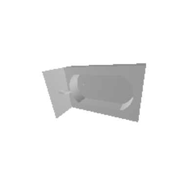
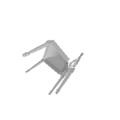
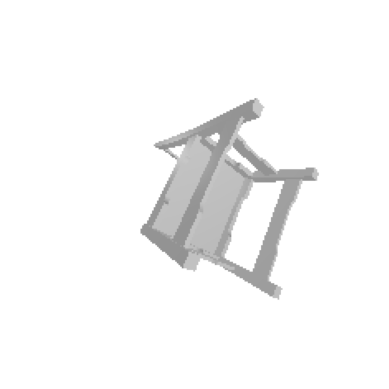
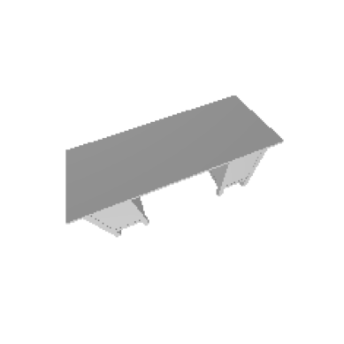
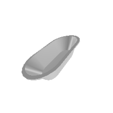
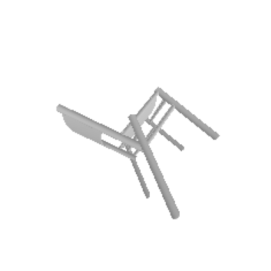
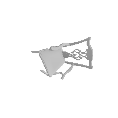
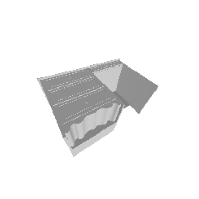
Currently, most SOTAs [52, 17, 55, 45, 41] explore transferring Contrastive Language-Image Pre-training (CLIP) [32] to 3D classification. Their general pipeline is projecting 3D objects to 2D depth maps and then matching the text and image features via CLIP. These methods are all based on the assumption that 3D objects are in aligned poses. However, objects in the real world are actually in open poses, such as an overturned chair or a flying bird. As shown in Fig. 1, SOTAs perform poorly when the aligned 3D object is modified to the open pose case. Furthermore, the emergence of CLIP has primarily accelerated the development of embedding methods in 3D zero-shot. However, in the field of 3D zero-shot, there are two mainstream approaches: embedding methods and generative methods [13, 2, 22], where generative methods remain largely under-explored.

In this paper, we make a first study on a more challenging yet practical task of 3D zero-shot classification aiming to recognize 3D objects in open poses. We rotate randomly each sample in the ModelNet10 [43] and McGill [37] datasets to obtain open-pose datasets ModelNet10^‡ and McGill^‡. Due to the uncertain pose, the selection of projection angles becomes a crucial matter. In this regard, we design a concise optimization algorithm to search and refine an ideal pose, significantly improving 3D open-pose zero-shot classification. Specifically, inspired by the principal component analysis, we perform a feature decomposition of the 3D object’s coordinates to obtain three eigenvectors. With a settled distance, we initially position the projection camera along the eigenvector direction that corresponds to the minimum variance, as a preliminary optimization of the projection angle. Furthermore, we propose to refine the angle by referencing the derivative of the matching degree with respect to it.

In addition, the pre-trained stable diffusion [35, 38], a generative model, has exhibited remarkable potential in the 2D zero-shot classification [20, 9]. However, a noteworthy unexplored territory remains in whether the 2D diffusion model can be extended to 3D recognition. We make the first attempt to bridge the 2D pre-trained diffusion model as a classifier to classify the 3D objects without additional training. This endeavor also expands the approach of applying 2D generative models to 3D zero-shot tasks. In detail, besides the depth map and rendered image, we adopt the edge image to obtain multiple styles of projections. With well-designed semantic descriptions, we input these images into the diffusion classifier [20] to attain a matching degree for classification. A series of experiments lay the groundwork for the diffusion transfer and confirm the effectiveness of our method. Especially, our approach achieves the state-of-the-art both on the 3D open pose dataset ModelNet10^‡, McGill^‡, and aligned pose dataset ModelNet10. The contributions of our work can be summarized as follows:

• We propose a more challenging benchmark for 3D zero-shot classification, recognizing 3D objects with open poses. Echoing our benchmark, we develop two open pose datasets ModelNet10^‡ and McGill^‡ for unified validation.

• We examine on the open pose benchmark current state-of-the-art methods, all of which lead to poor performance. Moreover, we design a concise angle-refinement mechanism to conquer it initially: our model achieves a substantial improvement on both ModelNet10^‡ and McGill^‡.

• To our best knowledge, we make the first attempt to bridge 2D diffusion as a classifier with 3D zero-shot classification, which expands the approach of generative-based 3D zero-shot model by leveraging 2D knowledge. Additionally, we propose to employ edge images with well-designed semantic descriptions to transfer the diffusion model knowledge sufficiently.

2 Related Works

Classification in the 3D Domain: The mainstream deep learning methods for 3D classification can be divided into three categories [11]: point-based, voxel-based, and multi-view-based method. PointNet [30] is the first network to extract point cloud features and recognize 3D objects. Point-Transformer [53, 42] applies a transformer in the 3D domain, significantly improving classification performance. Moreover, Voxnet [21] proposes to adopt voxel representation to process point clouds. Based on this, MinkowskiNet [8] provides a sparse voxel convolution architecture. In addition, MVCNN [39] suggests projecting the 3D mesh category from multi-view and adopting the 2D networks for training. LRMV [49] predicts the score of each projection view to select images. Unlike these supervised learning methods, our work is positioned in the zero-shot classification, where new (unseen) classes occur during the test.

Zero-Shot Classification in the 2D Domain: The goal of conventional zero-shot learning tasks is to perform classification on a sample set from unseen categories [19]. Currently, there are two main approaches to solving zero-shot classification tasks in the 2D domain [48]: embedding methods [33, 54, 12, 51], and generative methods [20, 47]. The former aims to learn a specific feature space matching the samples and category descriptions, while the latter transforms the zero-shot classification task into a normal classification by generating pseudo samples for unseen categories.

Additionally, both the pre-trained image-text matching model CLIP [32] and the diffusion classifier [20] can accomplish classification tasks without utilizing the training set of the specific benchmark. As a result, these methods are also referred to as zero-shot models. However, it should be noted that their pre-training dataset may contain samples corresponding to classes within the target dataset. Thus, in a strict sense, these methods differ from conventional zero-shot models in classifying “unseen classes”. Nevertheless, when these models are used to assist in the zero-shot classification of 3D data, they can be strictly categorized as zero-shot methods, since no 3D samples are adopted during the training process.

Figure 2: Overview of Network

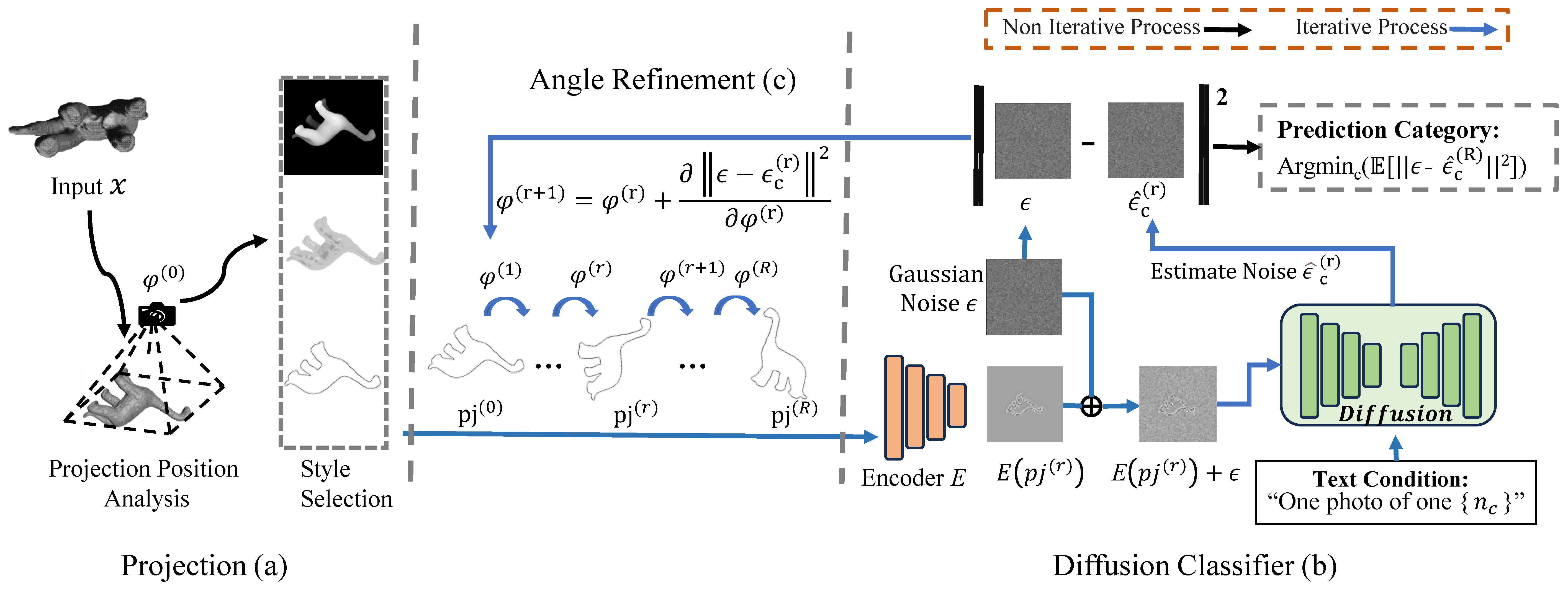
Zero-Shot Classification in the 3D Domain: Cheraghian et al. [5, 4, 6, 7] pioneers research on 3D zero-shot classification. They makes the first attempts in traditional [5], inductive [4], and transductive [6] zero-shot classification settings in the 3D domain, providing a standardized evaluation protocol for subsequent research work. Their proposed methods are based on text embedding (Word2Vect [23] & GloVe [29]) with two refinement loss functions [7]. On the other hand, 3DCZSL [25] takes an approach that considers the 3D zero-shot classification task from the perspective of geometric structure composition. However, it relies on point-wise component labels, which currently can only be satisfied by the PartNet dataset [24]. 3DGenZ [22] is proposed as the first generative 3D zero-shot classification network. It conducts Google searches for 100 images per class and utilizes a pre-trained classification network to obtain image representations for each category.

Furthermore, recent research [52, 17, 55, 31, 15, 28, 45, 46] has been concentrating on strategies to leverage the knowledge of the CLIP model to enhance performance on the 3D zero-shot classification. PointClip [52] is the pioneer of projecting 3D objects into 2D images and adopting CLIP to match the category. On the basis of this work, PointClipV2 [55] takes large-scale language models (GPT-3) [1] to automatically design a more descriptive 3D-semantic prompt. Moreover, Clip2Point [17] develops a network to narrow the domain gap between depth maps and realistic images. However, these methods are all built upon the assumption that objects are in aligned poses. In contrast, we introduce a more challenging task recognizing 3D objects in open poses. Additionally, we explore the performance of the diffusion model in 3D zero-shot classification, offering a significant boost for generative methods.

3 Methodology

3.1 Overview

The overall network architecture of our method is depicted in Fig. 2. Our method is based on a pre-trained diffusion model and does not require additional training. Therefore, this architecture is also directly used in the testing process with unseen class samples. It consists of three main parts: Projection (a), Diffusion Classifier (b), and Angle Refinement (c). First, with settled projection view corresponding to initialized projection angles, we transfer the projection images to three styles: depth, render, and edge images. Then, the diffusion classifier is applied to measure the similarity between the input image and each class. Based on the gradient of such similarity with respect to the projection angles, we iteratively optimize and refine the projection angles to obtain the most appropriate projection for recognizing each class.

3.2 Projection Styles

The primary data representations for 3D objects are point clouds and meshes. Our method takes both of these inputs into consideration. Owing to the sparsity of point clouds, their projection style differs significantly from that of meshes. To this end, we convert images projected from both point clouds and meshes into edge images for zero-shot classification. As shown in Fig. 3, two different input data formats result in distinct projected images, which are ultimately extracted into similar edge images.

Figure 3: Projection Styles

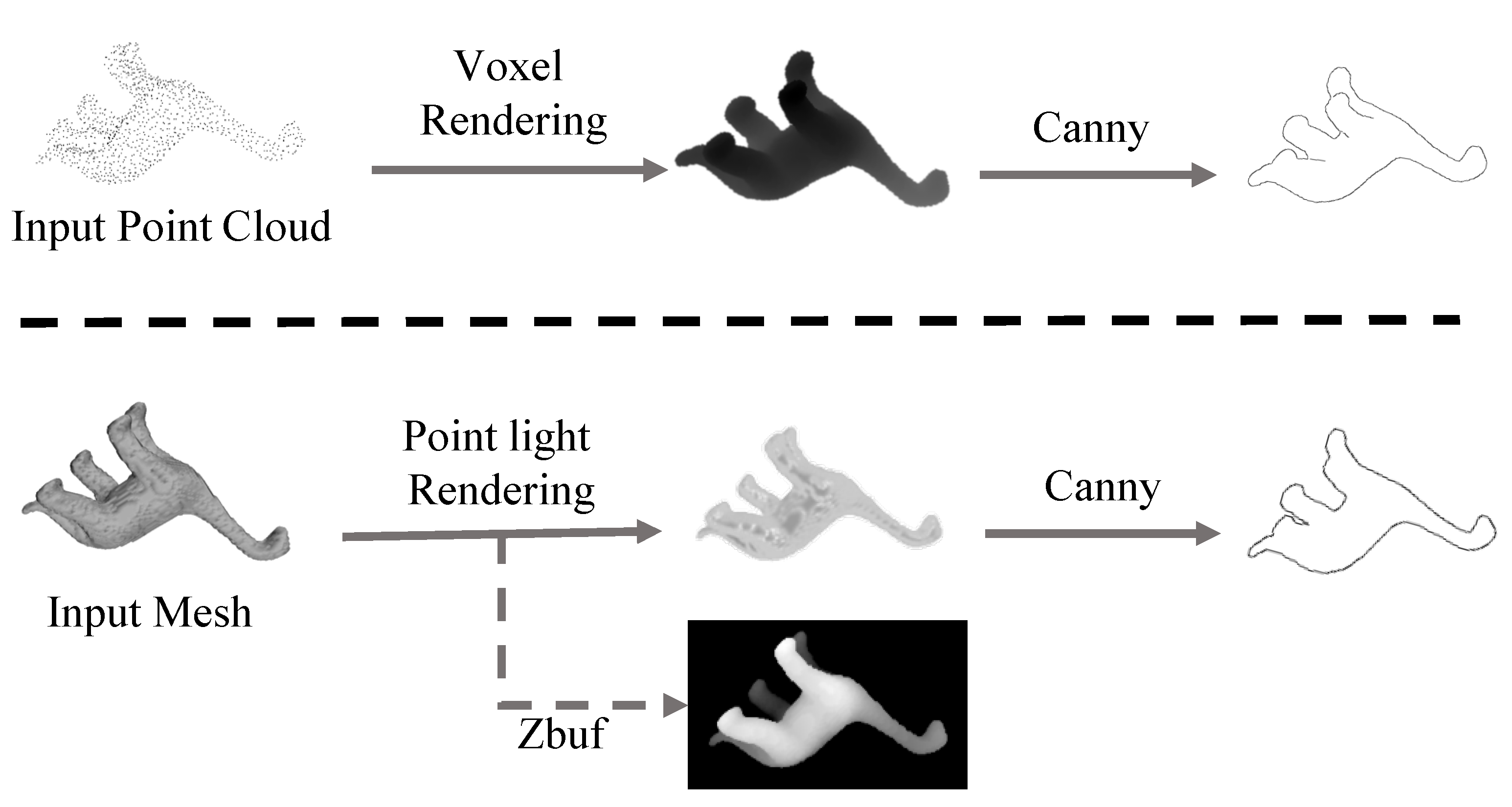
Specifically, when the input is point cloud data, direct projection yields a set of discrete pixels, making it challenging to represent its semantic information adequately. Following PointClipV2 [55], we adopt the voxel projection, which includes four steps: voxelize, densify, smooth, and squeeze, to attain the continuous pixel projection image. Furthermore, we utilize the canny algorithm to compute pixel gradients, thereby obtaining the edge image. On the other hand, mesh data includes additional face information, specifically triangular surfaces, compared to point cloud data. In this regard, we could directly achieve the continuous pixel projection image by point light projecting. To simulate parallel light, we position the point light source far away from the camera and the 3D mesh. To address noises on the surface of mesh data, we increase the Canny gradient threshold to eliminate this impact, which also results in the removal of some detailed information. For instance, the edge image of the mesh lacks the boundary of the legs compared to the edge image of the point cloud in Fig. 3.

3.3 Revisit of Diffusion Classifier

Given a clean feature sample $\bm{f_{0}}$ and a variance schedule $\beta_{1},...,\beta_{T}$, a Markov chain that gradually adds Gaussian noise to the data can be defined as follows:

$$q(\bm{f_{t}}|\bm{f_{t-1}})=\mathcal{N}(\bm{f_{t}};\sqrt{1-\beta_{t}}\bm{f_{t-1}},\beta_{t}\bm{I}).$$ (1)

The denoising diffusion probabilistic models [35] learn the reverse process $p_{\theta}(\bm{f_{t-1}}|\bm{f_{t}},s)$ with the corresponding semantic description $s$. Typically, the diffusion model can be interpreted as a denoising autoencoder $\bm{\epsilon_{\theta}}(\bm{f_{t}},t,s)$ with a training target minimizing the objective function

$$L_{DM}=\mathbb{E}_{\bm{f_{0}},\bm{\epsilon}\sim\mathcal{N}(\bm{0},\bm{I}),t}\left[\|\bm{\epsilon}-\bm{\epsilon_{\theta}}(\bm{f_{t}},t,s)\|^{2}_{2}\right].$$ (2)

In Diffusion Classifier [20], the posterior probability of the latent feature of the sample conditioned to the specific semantic is calculated based on the denoising performance, thus enabling the classification task. With a semantic description constructor $S(c)$ for each class and a 2D feature extractor $\bm{\epsilon_{\theta}}()$, such probability can be approximately estimated as follows:

$$p_{\theta}(c|\bm{f_{0}})=\frac{\exp\left\{-\mathbb{E}_{t,\bm{\epsilon}}\left[\|\bm{\epsilon}-\bm{\epsilon_{\theta}}(\bm{f_{t}},t,S(c))\|^{2}_{2}\right]\right\}}{\sum_{j}\exp\left\{-\mathbb{E}_{t,\bm{\epsilon}}\left[\|\bm{\epsilon}-\bm{\epsilon_{\theta}}(\bm{f_{t}},t,S(j))\|^{2}_{2}\right]\right\}}.$$ (3)

Here, we directly adopt such a pre-trained diffusion framework with the encoder $E()$. Since projection function $P_{k}()$ with style $k\in K$ and angles $\bm{\varphi}$ are considered in our framework, we define the semantic-image matching degree with the latent denoising module as below:

$${M\!D}_{\bm{\theta},K}(\bm{x},\bm{\varphi},c) =\exp\left\{-\mathbb{E}_{t,\bm{\epsilon},k}\left[\|\bm{\epsilon}-\bm{\hat{\epsilon}}_{\bm{\theta},k}(\bm{x},\bm{\varphi},c)\|^{2}_{2}\right]\right\}$$ (4)

$$\bm{\hat{\epsilon}}_{\bm{\theta},k}(\bm{x},\bm{\varphi},c) =\bm{\epsilon_{\theta}}\left(\bm{f}_{t,k}\left(\bm{x},\bm{\varphi}\right),t,S_{k}\left(c\right)\right),$$

$$\bm{f}_{t,k}\left(\bm{x},\bm{\varphi}\right) =\sqrt{\bar{\alpha}_{t}}E\left(P_{k}\left(\bm{x},\bm{\varphi}\right)\right)+\sqrt{1-\bar{\alpha}_{t}}\bm{\epsilon}$$

where followed by [16, 35], $\alpha_{t}=1-\beta_{t}$, $\bar{\alpha}_{t}=\prod_{i}^{t}\alpha_{t}$ is defined to construct the noised feature for timestep $t$. A higher value of this matching degree indicates better performance of the denoising module, as the expectation of the difference between actual and predicted noises becomes closer. Then, the following estimated probability and prediction for a 3D point that cloud sample under a single projection angle can be attained:

$$p_{\bm{\theta},K}(c|\bm{x},\bm{\varphi})=\frac{{M\!D}_{\bm{\theta},K}(\bm{x},\bm{\varphi},c)}{\sum_{j}{M\!D}_{\bm{\theta},K}(\bm{x},\bm{\varphi},j)}\\$$ (5)

$$\hat{y}=\underset{c}{\arg\max}\ p_{\bm{\theta},K}(c|\bm{x},\bm{\varphi}).$$ (6)

More details about the constructed semantic descriptions for the three projection types can be found in Section 4.4.

3.4 Projection Angle Update

3.4.1 Basic Projection Methods

Figure 4: Basic Projection Methods

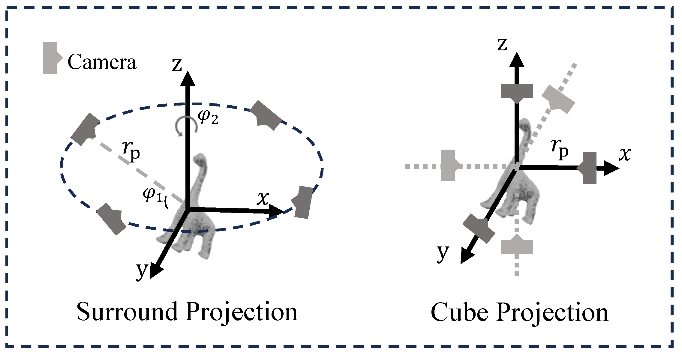
Existing projection-based 3D zero-shot classification methods all adopt the surround or cube projection, as shown in Fig. 5. Regarding surround projection, the camera is positioned obliquely above the object, which is adjusted by an angle $\varphi_{1}$ measuring the camera’s inclination with respect to the x-y plane. The multi-view images are obtained by changing the azimuthal angle $\varphi_{2}$ of the camera’s projection on the x-y plane relative to the x-axis. On the other hand, cube projection places the camera along the six directions of the three-dimensional coordinate axis. All cameras are oriented towards the center of the object and at a distance $r_{p}$ from the object. Both surround and cube projections do not change the object pose but only the camera position. In this regard, these two methods could get the appropriate view for the open pose 3D objects by adjusting the hyperparameters.

3.4.2 Iterative Angle Refinement Mechanism

To enhance the adaptability of the semantic-image matching framework to unaligned 3D point cloud data, the appropriate projection angles are indispensable. Here, we use the same angles described for surround projection. The pursuit of applying projection angles to maximize the prediction probability for each class is not rigorous, as a high probability for a particular class might be due to extremely low matching degrees with other classes under that angle. In this case, we propose an iterative angle refinement module employing the projection angles $\bm{\varphi}_{c}=\left[\varphi_{c,1},\varphi_{c,2}\right]$, maximizing the semantic-image matching degrees for each class $c$. The proposed module will lead to a more reasonable estimated probability as below:

$$p^{*}_{\bm{\theta},K}(c|\bm{x})=\frac{{M\!D}_{\bm{\theta},K}(\bm{x},\bm{\varphi}_{c},c)}{\sum_{j}{M\!D}_{\bm{\theta},K}(\bm{x},\bm{\varphi}_{j},j)}\\$$ (7)

$$\bm{\varphi}_{c}=\underset{\bm{\varphi}}{\arg\max}\ {M\!D}_{\bm{\theta},K}(\bm{x},\bm{\varphi},c).$$ (8)

As long as both the projection and semantic-image matching processes are differentiable, we can determine the projection angles with the highest matching degree for each class using the gradient descent algorithm. Given an initial projection angle vector $\bm{\varphi}^{(0)}$, the entire iterative optimization process with a series of refined scales $\left[\bm{\eta}_{r}\right]$ is presented as follows:

$$\bm{\varphi}_{c}^{(0)} =\bm{\varphi}^{(0)}$$ (9)

$$\bm{\varphi}_{c}^{(r+1)} =\bm{\varphi}_{c}^{(r)}+\bm{\eta}_{r}\cdot{sign}\left(\frac{\partial{M\!D}_{\bm{\theta},K}(\bm{x},\bm{\varphi}_{c}^{(r)},c)}{\partial\bm{\varphi}_{c}^{(r)}}\right).$$

After optimizing for $R$ steps, we use the estimated affine angle of each category $\widehat{\bm{\varphi}}_{c}=\bm{\varphi}_{c}^{(R)}$ to make the final classification prediction for the 3D point cloud samples as follows:

$$\widehat{y^{*}}=\underset{c}{\arg\max}\ \frac{{M\!D}_{\bm{\theta},K}(\bm{x},\widehat{\bm{\varphi}}_{c},c)}{\sum_{j}{M\!D}_{\bm{\theta},K}(\bm{x},\widehat{\bm{\varphi}}_{j},j)}.$$ (10)

However, the distribution of the matching degree calculated by the pre-trained model is typically not smooth in the projection angles space, and some semantic image matching models have a huge number of parameters (such as the Stable Diffusion” used in this work). Such scenarios make the optimization impractical and computationally expensive.

Data: 3D objects with open pose: $\bm{x}$

   Semantic description for each class: $S(c)$

   Pre-trained diffusion framework: $\bm{\epsilon_{\theta}}(),E()$

   Project function for each style: $P_{k}()$

   Iterative number: $R$

   Class number: $C$

   Refine scales: $\left[\bm{\eta_{r}}\right]$

   Distance from the camera to the object: $r_{p}$

11:  Calculate the covariance matrix $\bm{\Sigma}$ through Eq. 11 and calculate its eigenvectors $\bm{e_{1}},\bm{e_{2}},\bm{e_{3}}$ 22:  Establish a new coordinate system and obtain the coordinates $\bm{x^{\prime}}$ through Eq. 12 3:  for $c$ $\mathbf{in}$ range($C$) do 4:     Initialize the projection angle $\bm{\varphi}_{c}^{(0)}$ = 0 5:     for  $r$ $\mathbf{in}$ range($R$) do 6:        Sample random Gaussian noises $\bm{\epsilon}$ and calculate the matching dgree ${M\!D}_{\bm{\theta},K}(\bm{x^{\prime}},\bm{\varphi}_{c}^{(r)},c)$ through Eq. 4 7:        Calculate the partial derivative of matching degree and update the $\bm{\varphi}_{c}^{(r)}$ through Eq. 9 8:     end for 9:     Calculate the matching dgree ${M\!D}_{\bm{\theta},K}(\bm{x^{\prime}},\bm{\varphi}_{c}^{(R)},c)$ through Eq. 4 10:  end for 11:  Obtain the final prediction $\widehat{y^{*}}$ through Eq. 10 12:  return predicted label $\widehat{y^{*}}$

Algorithm 1 Iterative Angle Refinement Mechanism On Diffusion Classifier

To overcome these challenges, we introduce a more straightforward strategy to simplify the entire optimization process. First, we normalize and translate the sample coordinates to the coordinate origin to obtain the covariance matrix $\bm{\Sigma}$:

$$\bm{\Sigma}=(\bm{x}^{T}\cdot\bm{x})/N,\quad\bm{\Sigma}\in\mathbb{R}^{3\times 3},$$ (11)

where $\bm{x}$ and $N$ stand for the coordinates and the number of the vertexes in a sample. By eigenvalue decomposition to this matrix $\bm{\Sigma}$, we can obtain the three eigenvectors of this covariance matrix: $\bm{e_{1}},\bm{e_{2}},\bm{e_{3}}\in\mathbb{R}^{1\times 3}$. Then, we can establish a new coordinate system for the sample, resulting in the coordinates as follows:

$$\bm{x^{\prime}}=\bm{x}\cdot\left[\bm{e_{1}},\bm{e_{2}},\bm{e_{3}}\right].$$ (12)

According to principal component analysis, in the newly established coordinate system, fixing the camera on the z-axis in the new coordinates ensures the largest variance in each dimension of the projected image. Such a view may lead to more classification information being captured. Moreover, this operation reduces the projection angles variable from two dimensions to one (only the azimuthal angle $\varphi_{c,2}$). Instead of applying this rotation angle directly to the 3D data, it can be equivalently applied to the projected image. After this initial adjustment of the projection angle, we can continue to refine the angle through the gradient, as previously introduced, within a more simplified single-dimension case. The detailed steps for the proposed angle refinement strategy are presented in Algorithm 1.

4 Experiments

4.1 Experiment setting

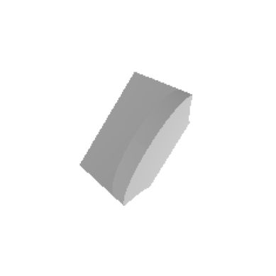
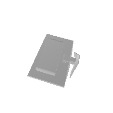
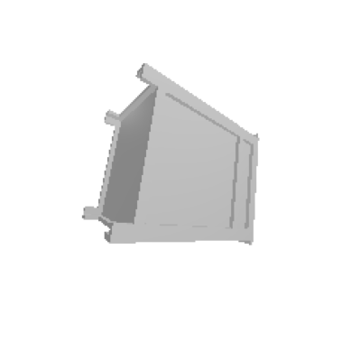
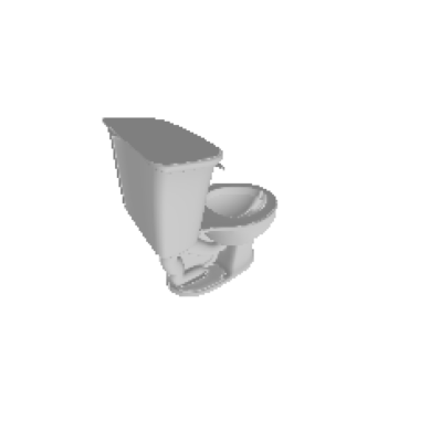
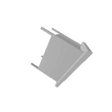
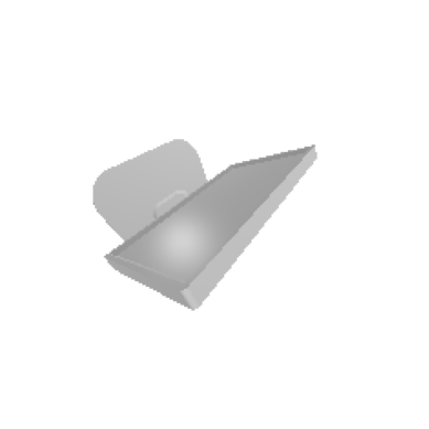
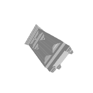
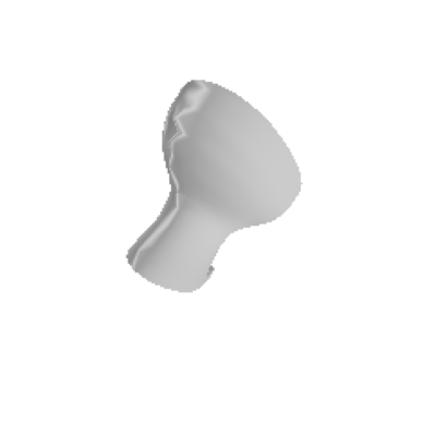
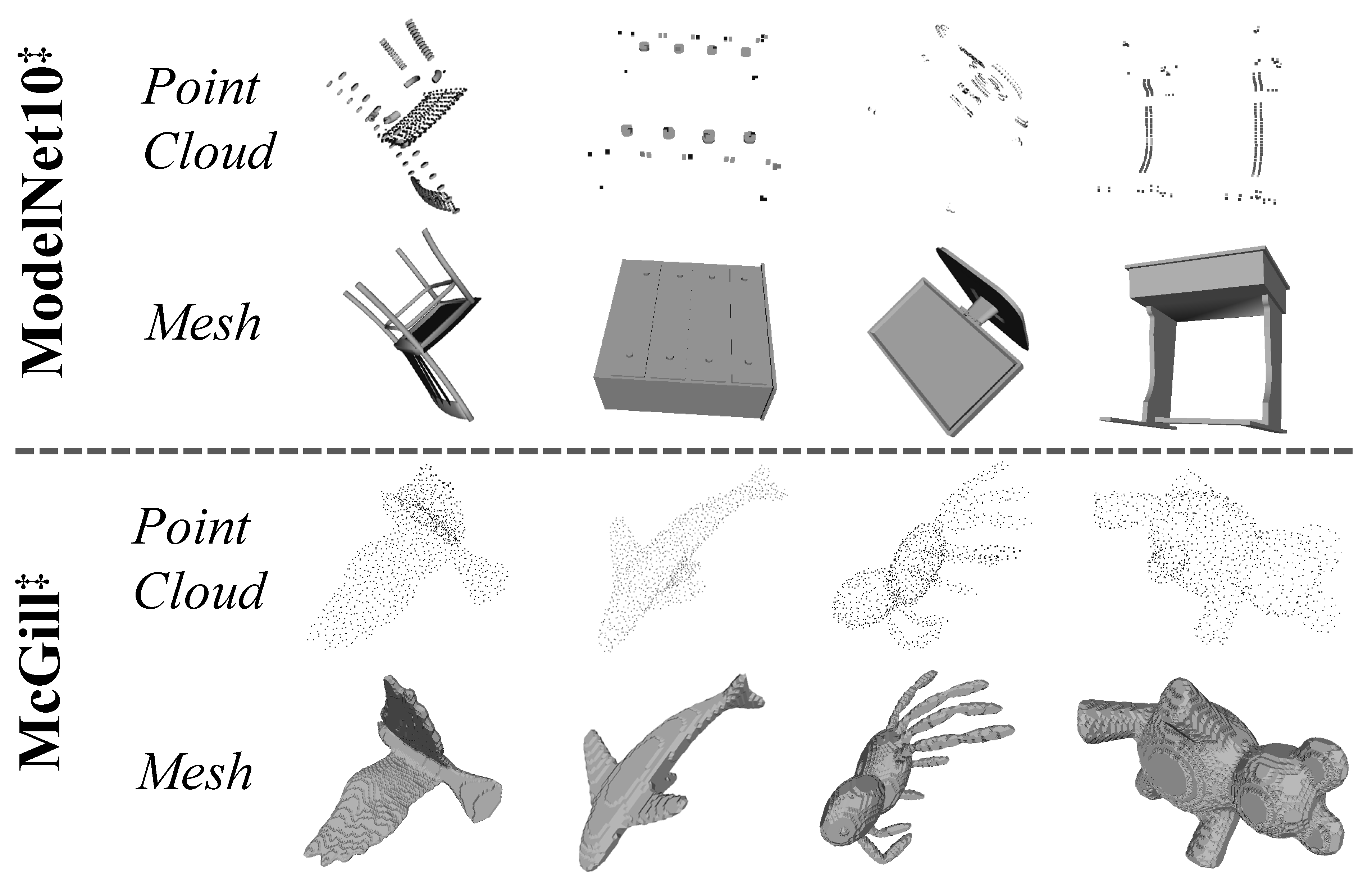
Datasets. We evaluate our method on our open pose benchmarks: ModelNet10^‡ and McGill^‡. These two datasets are sourced from the ModelNet10 [43] and McGill [37] datasets, respectively. ModelNet10 is a subset of ModeNet40 [43], a classic classification dataset including furniture categories, such as tables, chairs, and displays, with all samples well-aligned. It contains 4,899 CAD models with 10 different classes, split into 3,991 training and 908 testing samples. McGill primarily features animal categories such as birds and dolphins, along with other unique categories like hands. It includes 115 unaligned test samples with 14 categories, where the overlapping categories with ModelNet40 are removed. We rotate each sample in ModelNet10 and McGill to obtain the ModelNet10^‡ and McGill^‡, respectively. Examples of the rotated samples are illustrated in Fig. 5 Although the samples in McGill are inherently unaligned, the range of their rotational angles is limited, lacking sufficient randomness to illustrate the open pose issue effectively. Therefore, we also applied random angle rotations to them.

Figure 5: Examples of samples from ModelNet10^‡ and McGill^‡.

Evaluation Metric. Following existing SOTAs [7, 13, 31], we take the top-1 accuracy as the recognition performance. In other words, the class with the highest predicted probability should be the true class. For our method, the higher the matching degree, the greater the probability of the class. In this case, the output of Clip can also be regarded as the matching degree. Thus, the proposed angle refinement mechanism can effectively apply to CLIP-based methods. Such an algorithm is provided in the Supplementary Material. We also introduce mAcc as an evaluation metric, which calculates the average accuracy across all categories, which better reflects the model’s classification performance for different categories.

Implementation Details. We conduct our end-to-end inference process on one single RTX3090 card. The stable diffusion [35] is adopted as the 2D pre-trained model to predict the noise. Following stable diffusion, we set the seed to 42. For hyperparameters of the diffusion classifier, we tune timesteps and trails empirically as 600 and 30, respectively. The relevant sensitivity analysis can be found in the Supplementary Material. Furthermore, we adjust the project camera distance $r_{p}$ as 2.2 and the angle refinements parameters $R$ and $\left[\bm{\eta_{r}}\right]$ as 10 and $\left[20,18,16,...,2\right]$. In terms of projection, we employ single-point light source projection of PyTorch3D [34] for mesh samples and utilize voxel projection for the point cloud samples.

4.2 Comparison to SOTAs

We examine four recent SOTAs: PointClip [52], ReconClip [31] , Clip2Point [17], PointClipV2 [55] on our open pose benchmark ModelNet10^‡ and McGill^‡ for 3D zero-shot classification. All the reproduction codes are sourced from the official GitHub repository of the respective papers. Since ReconClip and Clip2Point adopt the mesh images for the additional training, we report our method results for both point clouds and meshes. Detailed results are reported in Tab. 1 and Tab. 2. To more comprehensively validate our proposed angle refinement mechanism, we also used CLIP as a classifier under the same settings to verify the results. The experimental outcomes can be found in the Supplementary Material.

Results on the Open Pose 3D Zero-shot ModelNet10^‡. As shown in Tab. 1, our angle-refinement mechanism achieves a new benchmark on the open pose ModelNet10^‡. In contrast, our method achieves a significant improvement, especially when the mesh information is supplemented. Note that the point cloud in ModelNet10^‡ is incomplete, making it more challenging to classify with zero-shot compared to McGill^‡. Particularly, samples in this benchmark tend to be boxy and symmetrical, with minimal variance between some classes, thus making the task really tough in an open pose scenario.

	Venue	Acc	mAcc
PointClip [52]	CVPR’2022	17.7	16.4
ReconClip [31]	ICML’2023	15.6	14.3
Clip2Point [17]	ICCV’2023	19.7	18.1
PointClipV2 [55]	ICCV’2023	19.9	18.2
Ours-Point	–	20.7	19.0
Ours-Mesh	–	22.6	21.7

Table 1: Comparison to current SOTAs on the Open Pose 3D Zero-shot ModelNet10^‡.

Result on the Open Pose 3D Zero-shot McGill^‡. We report our method results on open pose McGill^‡ in Tab. 2. Obviously, our method demonstrates high performance, showing 11.3%, and 15.8% improvements on Acc and mAcc, respectively. Moreover, there are some unsmooth surfaces over the mesh in McGill^‡, these unsmooth surfaces interfere with the edge extraction process by canny. To this end, the results of Ours-Mesh are lower than Ours-Point.

	Venue	Acc	mAcc
PointClip [52]	CVPR’2022	12.2	13.3
ReconClip [31]	ICML’2023	15.7	17.3
Clip2Point [17]	ICCV’2023	14.8	17.4
PointClipV2 [55]	ICCV’2023	27.8	28.9
Ours-Point	–	39.1	44.7
Ours-Mesh	–	35.7	39.5

Table 2: Comparison to existing SOTAs on the Open Pose 3D Zero-shot McGill^‡.

	Ant	Bird	Crab	Dino.	Dolp.	Fish	Hand	Octo.	Plier	Quad.	Snake	Spec.	Spider	Teddy	Acc	mAcc
Top View	0.0	28.6	0.0	0.0	0.0	0.0	0.0	0.0	42.9	0.0	0.0	11.1	9.1	0.0	6.1	6.6
Cube	0.0	57.1	0.0	0.0	100.0	0.0	14.3	25.0	85.7	0.0	66.7	0.0	18.2	0.0	21.7	26.2
Surround	0.0	57.1	0.0	0.0	75.0	12.5	57.1	37.5	100.0	9.1	55.6	0.0	9.1	0.0	25.2	29.5
Ours	0.0	71.4	10.0	0.0	100.0	12.5	71.4	37.5	71.4	27.3	77.8	0.0	45.5	28.6	35.7	39.5

Table 3: Projection Angle Update on the McGill^‡. In order to reduce the length of the table, we take abbreviations for some category names: Dino. vs Dinosaur, Dolp. vs Dolphin, Octo. vs Octopus, Quad. vs Quadruple, Spect. vs Spectacle.

4.3 Analysis on Views Selection

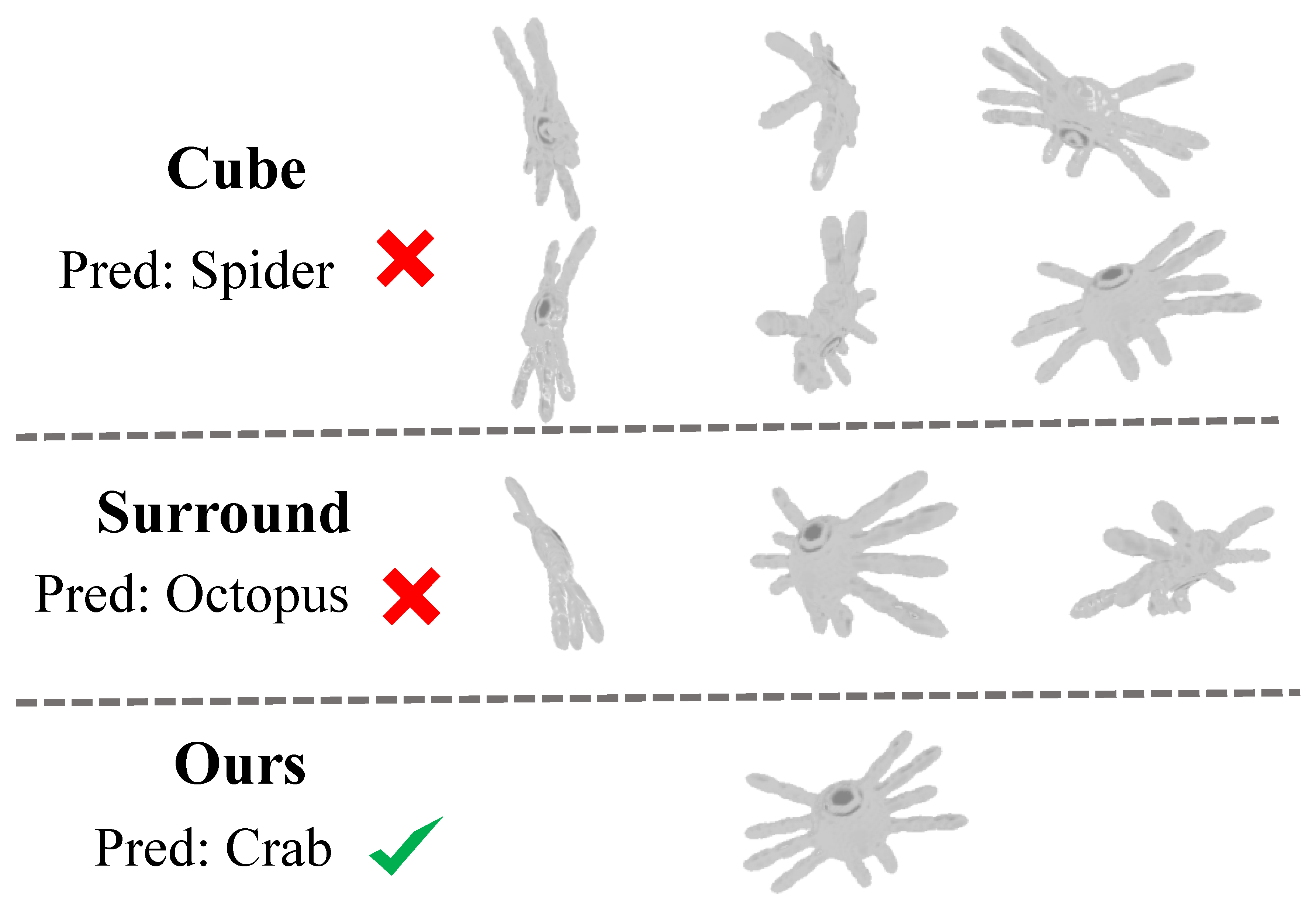
We contrast our iterative angle refinement mechanism with the commonly used SOTA projection methods, Cube and Surround Views. The visualization results of these methods for a single sample, corresponding to angles and projections, along with the final predictions, are displayed in Fig. 6. Additionally, we include a settled single-view approach using only the top view for further context. The results, detailed in Tab 3, reveal significant disparities. In open pose scenarios, the fixed single-view perspective yields notably poor results, with an accuracy of merely 6.6%. While the Cube and Surround methods, as multi-view ensembled approaches, indeed show improvement over a single-view perspective, their performance is still hindered by the randomness inherent in open poses. In contrast, our angle refinement mechanism offers a more advantageous approach to selecting views conducive to classification. It leads to substantial gains, as evidenced by our method showing 10.5% and 10.0% improvements in Acc and mAcc, respectively, on the open pose McGill^‡ benchmark.

Figure 6: Views Selection with the corresponding Prediction.

4.4 Analysis on Bridging 2D Diffusion

Different from current SOTAs, we are the first to adopt 2D pre-trained diffusion as the 3D zero-shot classification instead of Clip. Therefore, in this section, we verify its performance on the generic aligned pose ModelNet10 to hint at its potential. We specifically choose the aligned pose for validation due to the corresponding superior and more stable performance, as verifying under this scenario can more convincingly demonstrate the effectiveness.

Comparisons on the Aligned Pose Scenario. In this traditional setting, all objects are oriented in the same direction. To this end, we adopt the surrounding projection and set the $\varphi_{1}$,$\varphi_{2}$ as 60, 210 respectively to attain the appropriate projection view. The detailed comparison results are reported in Tab. 4. Obviously, our diffusion-based method outperforms the state-of-the-art by 6.8% on Acc. Furthermore, existing SOTAs [52, 31, 17, 55] bridge 2D Clip to the 3D zero-shot classification, making a vital improvement for the embedding method. In contrast, our work bridges 2D Diffusion to the 3D zero-shot classification, energizing the generative model method with 44.9% improvement.

		Venve	Pre-training	Acc
E	MHPC [4]	BMVC’19		33.9
	TZSLPC [6]	WACV’20		23.5
	ZSL3D [7]	IJCV’22		32.5
	PointClip [52]	CVPR’22	✓	30.2
	ReconClip [31]	ICML’23	✓	75.6
	Clip2Point [17]	ICCV’23	✓	66.3
	PointClipV2 [55]	ICCV’23	✓	73.1
G	f-CLSWGAN [44]	TPAMI’18		13.7
	CADA-VAE [36]	CVPR’19		15.6
	TF-VAEGAN [27]	ECCV’20		27.2
	3DGenZ [22]	3DV’21		36.8
	CGRL [13]	PR’23		25.2
	Ours-Mesh	–	✓	82.4

Table 4: Comparison to SOTAs on the Aligned Pose 3D Zero-shot ModelNet10. E stands for embedding methods and G represents generative model methods.

Comparison on Prompts. To further explore the impact of semantic descriptions on the matching of various styled projections, we design multiple prompts for three style images: Render I. (Render Image), Depth I. (Depth Image), and Edge I. (Edge Image). We report the corresponding mACC results on ModelNet10 in Tab. 5 under the case that trails is 30 and $r_{p}$ is 2.2. Specifically,“one line-drawn [$n_{c}$]” is the best prompt for depth images, and “one model of [$n_{c}$] in linear composition” is the best prompt for render images, while “one edge map of one standalone [$n_{c}$] ” is the best prompt for edge images. Moreover, the edge images show the best results among the three types of images.

Prompts	Render I.	Depth I.	Edge I.
one model of [$n_{c}$]	69.3	58.8	72.3
one line-drawn [$n_{c}$]	69.9	59.8	72.0
one photo of one [$n_{c}$]	69.6	53.2	73.7
one photo of one standalone [$n_{c}$]	63.4	51.6	71.1
one depth map of one standalone [$n_{c}$]	67.2	48.5	77.4
one edge map of one standalone [$n_{c}$]	66.1	51.9	77.6
one render image of one standalone white [$n_{c}$]	68.0	55.6	66.3
one sketch photo of one standalone white [$n_{c}$]	65.8	53.0	74.7
one model of [$n_{c}$] in linear composition	73.5	59.5	73.5
one photo of one [$n_{c}$] in linear composition	73.1	59.7	73.7

Table 5: Prompts for Multiple Style Images. [$n_{c}$] stands for the name text of each category.

Comparison to the Clip Model. We compare the effectiveness of the diffusion classifier with that of the Clip classifier on ModelNet10. We only exchange the classifier and keep the same for all other conditions. The comparison mACC results are reported in Tab. 6. For the Clip model, we adopt four common structures of pre-trained model: Clip-VIT-B\16 [10], Clip-VIT-B\32 [10], Clip-ResNet50 [14], and Clip-ResNet101 [14]. Overall, Clip-VIT-B\16 takes the best performance among these Clip models. However, the diffusion classifier shows more powerful effectiveness, especially when the trail is equal to 30 (Tr.30).

Furthermore, the diffusion classifier is much slower than the Clip classifier. This is attributed to its more complex computational process. Theoretically, selecting a greater number of trials and timesteps in diffusion can lead to further enhancements in performance. Therefore, opting for the diffusion method implies a trade-off, where significant computational resources are expended to achieve performance gains.

	Render I.	Depth I.	Edge I.	Times (s)
Clip-VIT-B\16	54.7	59.7	34.2	0.025
Clip-VIT-B\32	49.6	52.7	38.0	0.028
Clip-ResNet50	45.2	41.9	37.5	0.037
Clip-ResNet101	48.4	54.3	40.8	0.042
Diffusion-Tr.10	66.2	53.5	70.4	8.771
Diffusion-Tr.20	71.6	58.6	74.3	17.461
Diffusion-Tr.30	73.5	59.8	77.6	26.078

Table 6: Comparison to the Clip Model. Times denotes the averaged inference time of a single projected image.

Ablation on Projection Styles. We conduct the ablation studies of the three style images (Render, Depth, Edge) for both the Clip and Diffusion models on the ModelNet10 dataset. The results are reported in Tab. 6& 7. The Clip model shows the best performance for the depth images and the worst for the edge images, whereas the diffusion model performs reversely. Moreover, we explore the ensemble of these styles to achieve better performance. Specifically, as introduced in Section 3.3, the ensemble stands for taking the average over projection styles when calculating the matching degree. From Tab. 7, the Clip model attains better mAcc results by combining render and depth images. On the other hand, the Diffusion model takes the best performance by combining render and edge images.

	Render	Depth	Edge	mACC
Clip-VIT-B\16	✓	✓		61.2
Clip-VIT-B\16		✓	✓	53.6
Clip-VIT-B\16	✓		✓	50.2
Clip-VIT-B\16	✓	✓	✓	53.6
Diffusion-Tr.30	✓	✓		73.2
Diffusion-Tr.30		✓	✓	79.4
Diffusion-Tr.30	✓		✓	81.7
Diffusion-Tr.30	✓	✓	✓	79.4

Table 7: Ablation on Projection Styles

5 Conclusion

This paper proposes a more challenging benchmark for 3D zero-shot classification to recognize unseen 3D objects with uncertain poses. Correspondingly, we design a concise angle-refinement mechanism to present our preliminary solution. This mechanism utilizes principal component analysis to attain the initial projection angle and adjusts it through the gradient of the matching degree for each category. Additionally, we pioneered the transfer of knowledge from pre-trained 2D diffusion models to 3D zero-shot classification, surpassing the state-of-the-art in aligned pose scenarios. However, our approach, being an initial exploration in open pose situations, does not achieve as remarkable results as in the aligned pose case. In our future work, we aim to improve our method for view selection to enhance effectiveness in open pose scenario of 3D zero-shot classification.

Supplementary Material

6 Iterative Angle Refinement Mechanism on Clip

Figure 7: Iterative Angle Refinement Mechanism on Clip

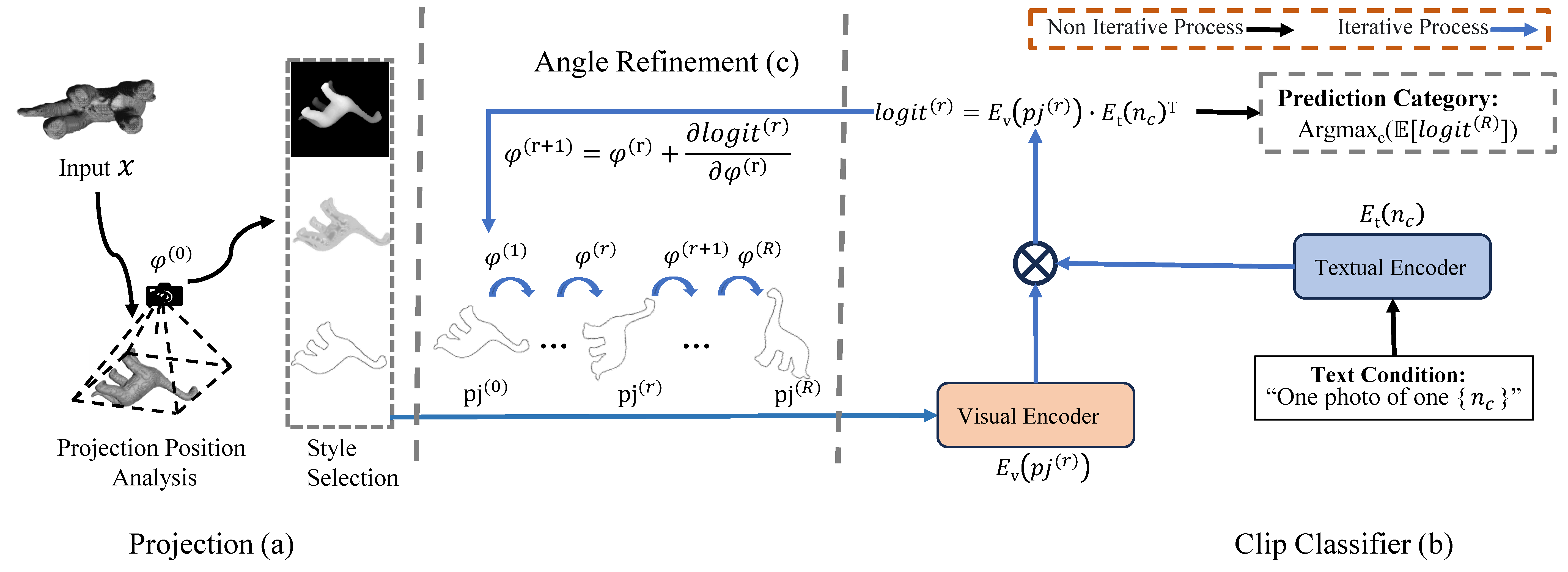
Our iterative angle refinement mechanism is applicable to both Diffusion and Clip classifiers. In the previous Section 3.4.2, we primarily introduced the effectiveness of the iterative angle refinement mechanism on the Diffusion classifier. In this section, we will further explore its extension on the Clip classifier. Since the output of the Clip, $logit=E_{v}\left(image\right)\cdot E_{v}\left(text\right)$, essentially measures the similarity between image and text inputs, the expectation of it can be regarded as the defined matching degree as below:

$$MD_{k}(\bm{x^{\prime}},\bm{\varphi}_{c}^{(r)},c)=\mathbb{E}_{k}\left[E_{v}\left(P_{k}\left(\bm{x},\bm{\phi}\right)\right)\cdot E_{t}\left(S_{k}\left(c\right)\right)\right].$$ (13)

Thereby, we can directly employ the proposed angle refinement mechanism to optimize the projection angles. Such process can be referenced shown in Fig. 7, we modify the Clip Classifier(b) and Angle Refinement(c) compared to the previous network Fig. 2. The detailed steps are presented in Algorithm 2.

Data: 3D objects with open pose: $\bm{x}$

   Semantic description for each class: $S(c)$

   Pre-trained Clip framework: $E_{v}(),E_{t}()$

   Project function for each style: $P_{k}()$

   Iterative number: $R$

   Class number: $C$

   Refine scales: $\left[\bm{\eta_{r}}\right]$

   Distance from the camera to the object: $r_{p}$

1

21:   Calculate the covariance matrix $\bm{\Sigma}$ through Eq. 11 and calculate its eigenvectors $\bm{e_{1}},\bm{e_{2}},\bm{e_{3}}$

32:   Establish a new coordinate system and obtain the coordinates $\bm{x^{\prime}}$ through Eq. 12

3:   for $c$ $\mathbf{in}$ range($C$) do

4:      Initialize the projection angle $\bm{\varphi}_{c}^{(0)}$ = 0

5:      for  $r$ $\mathbf{in}$ range($R$) do

6:         Calculate the matching dgree ${M\!D}_{K}(\bm{x^{\prime}},\bm{\varphi}_{c}^{(r)},c)$ through Eq. 13

7:         Calculate the partial derivative of matching degree and update the $\bm{\varphi}_{c}^{(r)}$ through Eq. 9

8:      end for

9:      Calculate the matching dgree ${M\!D}_{K}(\bm{x^{\prime}},\bm{\varphi}_{c}^{(R)},c)$ through Eq. 13

10:   end for

11:   Obtain the final prediction $\widehat{y^{*}}$ through Eq. 10

12:   return predicted label $\widehat{y^{*}}$

Algorithm 2 Iterative Angle Refinement Mechanism On Clip Classifier

6.1 Comparison to SOTAs

We present our results with Clip for the open-pose 3D zero-shot classification on ModelNet10^‡ in Tab. 8. As we observed, our method with Clip achieves the state-of-art with 6.0% mAcc improvement, compared to SOTAs. Due to the incomplete nature of the point cloud in ModelNet10^‡, Ours(Clip)-Point performance is lower compared to Ours(Clip)-Mesh. On the other hand, we also report our results on open pose 3D zero-shot McGill^‡ in Tab. 9. Our method still shows 3.3% mAcc improvement on this dataset, compared to SOTAs. Referring to the results from Tab. 1 &  2 in Section 4.2, our approach is effective for both the Clip and Diffusion Classifier.

	Venue	Acc	mAcc
PointClip [52]	CVPR’2022	17.7	16.4
ReconClip [31]	ICML’2023	15.6	14.3
Clip2Point [17]	ICCV’2023	19.7	18.1
PointClipV2 [55]	ICCV’2023	19.9	18.2
Ours(Clip)-Point	–	23.6	21.8
Ours(Clip)-Mesh	–	26.3	24.2

Table 8: Performance of the angle refinement mechanism with Clip compared to current SOTAS on ModelNet10^‡.

	Venue	Acc	mAcc
PointClip [52]	CVPR’2022	12.2	13.3
ReconClip [31]	ICML’2023	15.7	17.3
Clip2Point [17]	ICCV’2023	14.8	17.4
PointClipV2 [55]	ICCV’2023	27.8	28.9
Ours(Clip)-point	–	30.4	32.6
Ours(Clip)-mesh	–	28.7	32.2

Table 9: Performance of the angle refinement mechanism with Clip compared to current SOTAS on McGill^‡

7 Sensitivity Analysis for the Diffusion

Figure 8: Sensitivity Analysis on the Trail.

7.1 Sensitivity Analysis

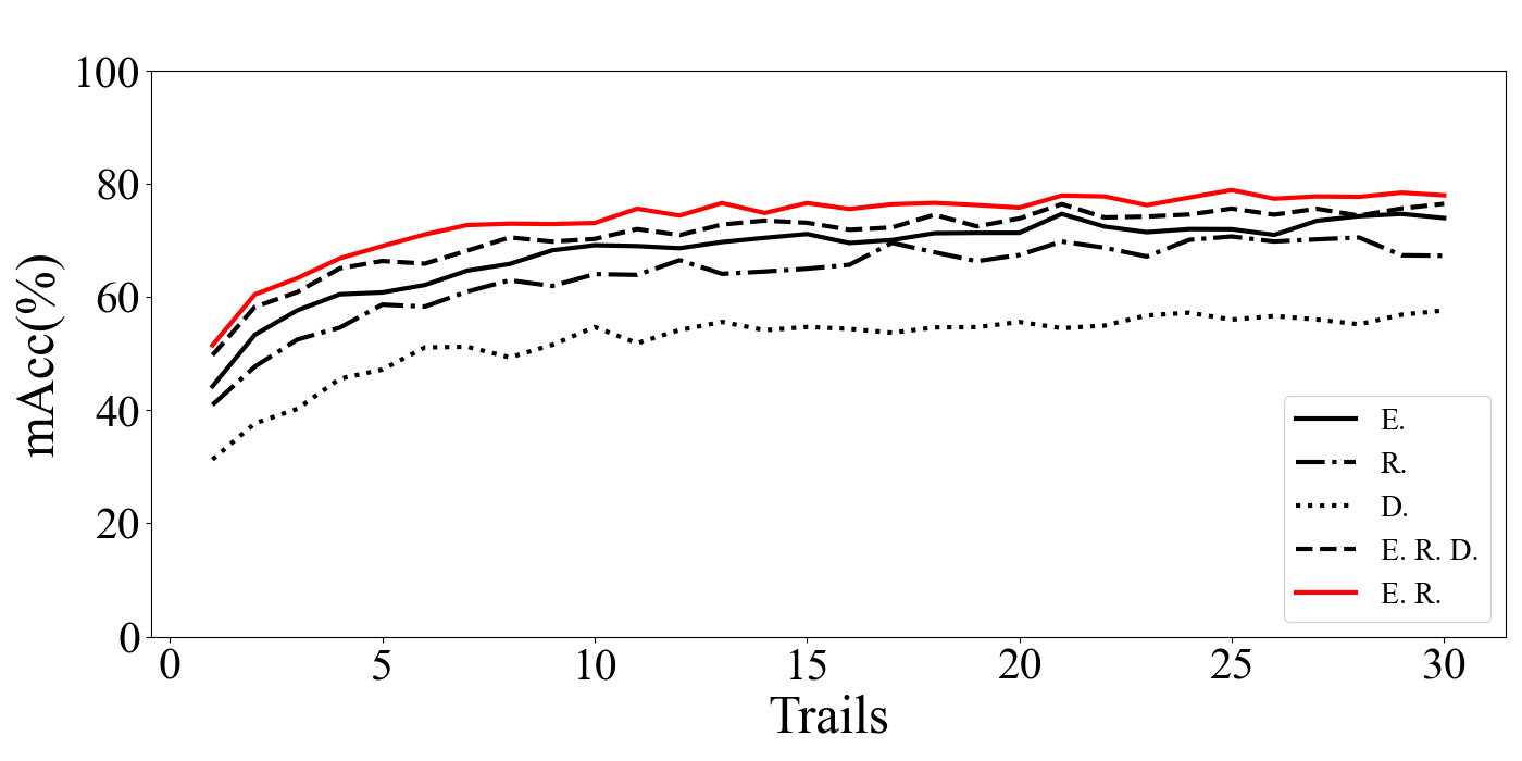
We conduct the sensitivity analysis on the two hyperparameters of the diffusion classifier: Timestep and Trail. In detail, we present the analysis results for render (R.), depth (D.), edge (E.), edge&render (E. R.), and edge&render&depth (E. R. D.) projection image input, where & denotes the ensemble results. Moreover, we fix the prompt as “one photo of one [$n_{c}$] ” on the aligned pose setting to compare the results fairly. As depicted in Fig. 8, when the value of the trail grows to 20, the performance of our model is basically stable. Furthermore, (E. R.) shows the best performance which echoes the Tab. 7. u

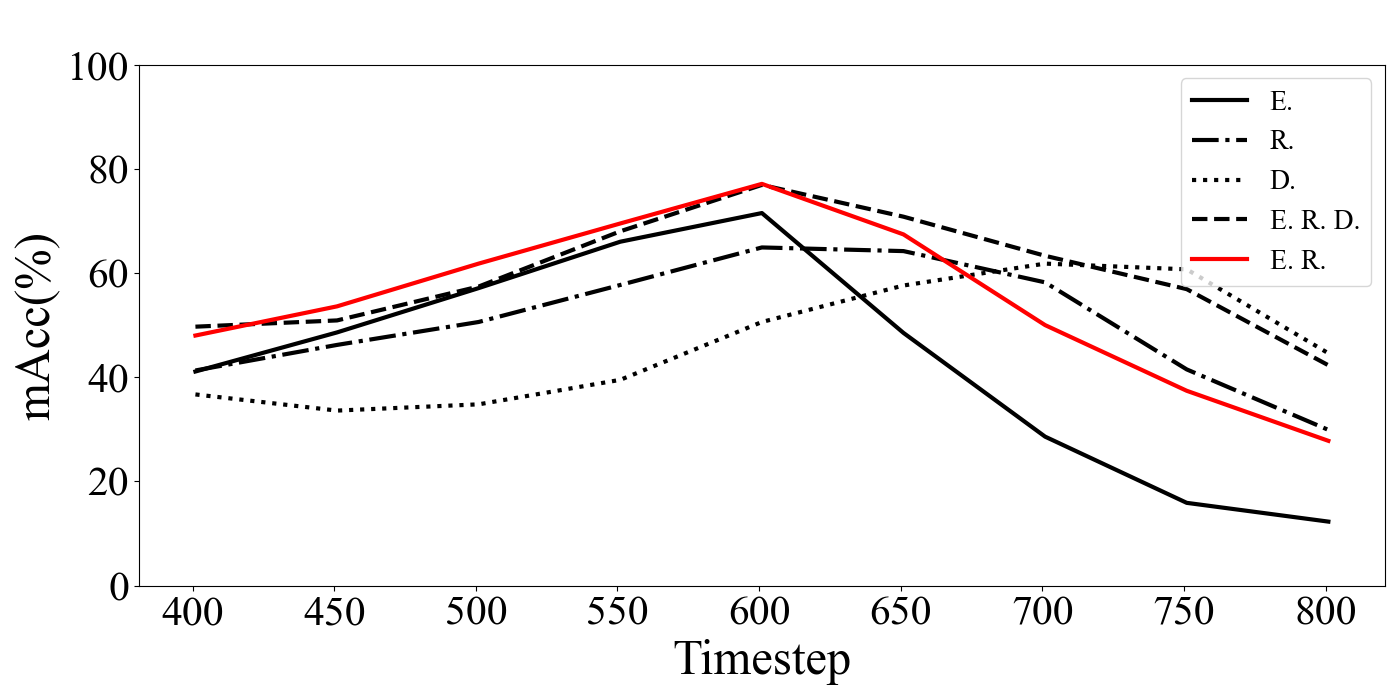
On the other hand, we report the results on the timestep in Fig. 9. Slightly different from the previous method [20], the best value of the timestep is around 600 instead of 550. When the timestep is less than 600, our 3D zero-shot classification performance is relatively stable. When the timestep equals 600, our model achieves optimal performance. However, when the timestep exceeds 650, the model’s performance deteriorates significantly. In summary, there is a range where our method is insensitive to these two hyperparameters.

Figure 9: Sensitivity Analysis on the Timestep.

8 Projection Visualization

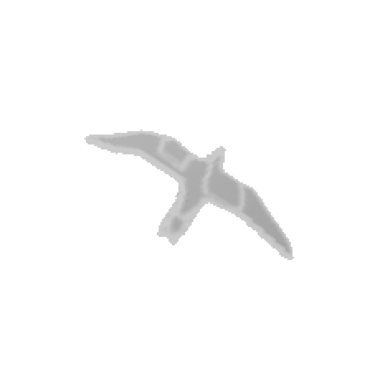
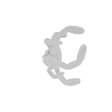
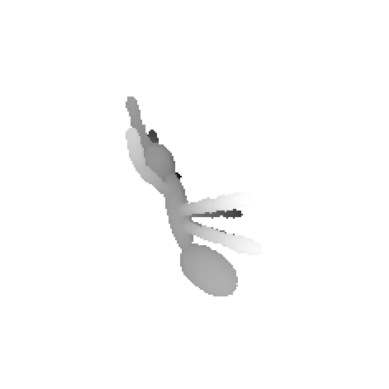
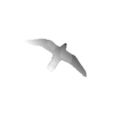
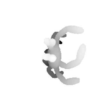
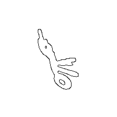
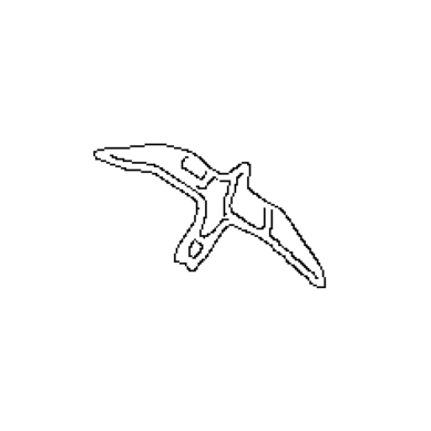
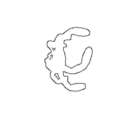
In this section, we provide more projection visualization results for three styles: render, depth, and edge images in Fig. 10. We adopt the frontal view in the Cube method to uniformly display.

Render

Depth

Edge

Figure 10: Projection Visualization

9 Open Pose 3D Zero-Shot Classification Benchmark

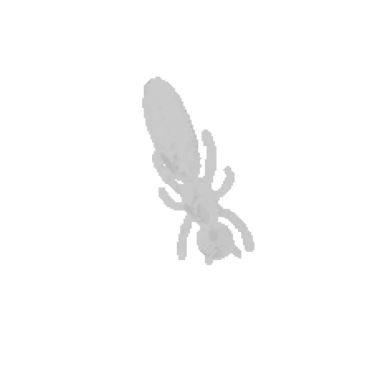
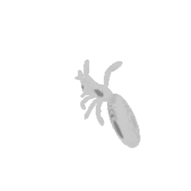
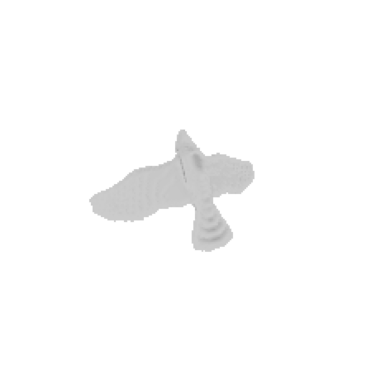
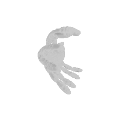
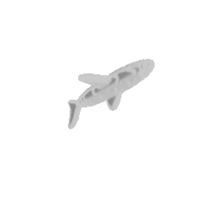
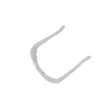
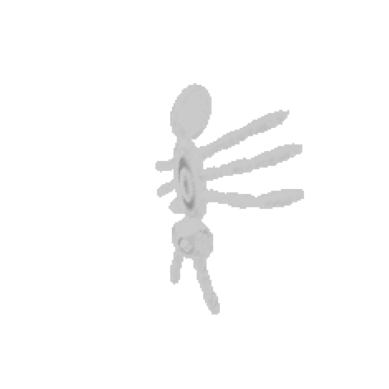
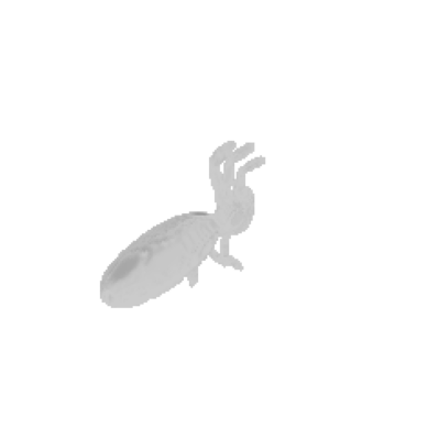
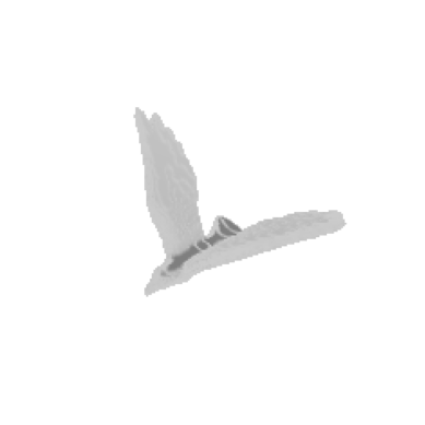
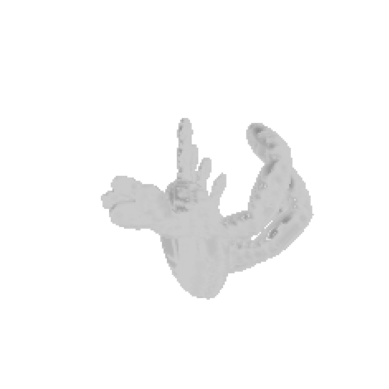
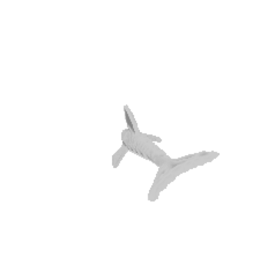
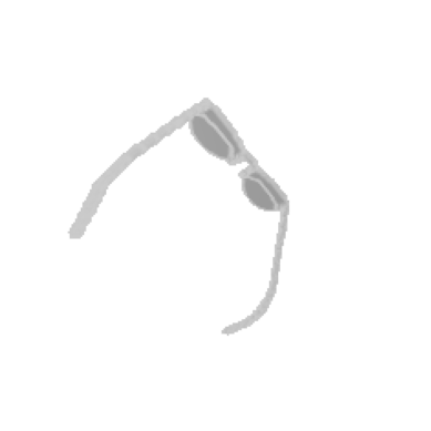
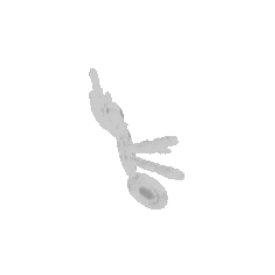
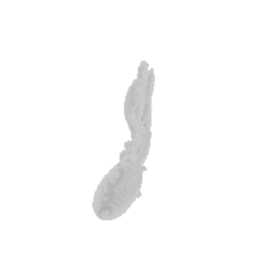
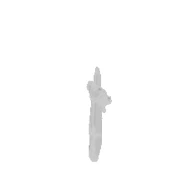
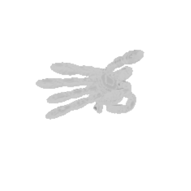
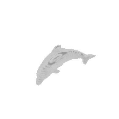
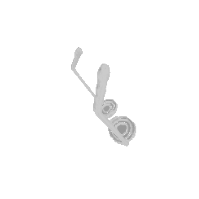
In this section, we provide visualizations of selected samples from our open pose benchmark McGill^‡ and ModelNet10^‡. As shown in Fig. 11 & 12, our benchmark provides diverse poses for each sample, making the 3D zero-shot task more realistic. We also adopt the frontal view in the Cube method to uniformly display.

9.1 McGill^‡

Figure 11: Selected Samples from McGill^‡

9.2 ModelNet10^‡

Figure 12: Selected Samples from ModelNet10^‡

References

- Brown et al. [2020] Tom B. Brown, Benjamin Mann, Nick Ryder, Melanie Subbiah, Jared Kaplan, Prafulla Dhariwal, Arvind Neelakantan, Pranav Shyam, Girish Sastry, Amanda Askell, Sandhini Agarwal, Ariel Herbert-Voss, Gretchen Krueger, Tom Henighan, Rewon Child, Aditya Ramesh, Daniel M. Ziegler, Jeffrey Wu, Clemens Winter, Christopher Hesse, Mark Chen, Eric Sigler, Mateusz Litwin, Scott Gray, Benjamin Chess, Jack Clark, Christopher Berner, Sam McCandlish, Alec Radford, Ilya Sutskever, and Dario Amodei. Language models are few-shot learners. In NeurIPS, pages 1877–1901, 2020.
- [2] Yiwen Cao, Yukun Su, Guosheng Lin, and Qingyao Wu. Mutex parts collaborative network for 3d point cloud zero-shot classification. SSRN.
- Chen et al. [2023] Jiajing Chen, Minmin Yang, and Senem Velipasalar. Viewnet: A novel projection-based backbone with view pooling for few-shot point cloud classification. In CVPR, pages 17652–17660, 2023.
- Cheraghian et al. [2019a] Ali Cheraghian, Shafin Rahman, Dylan Campbell, and Lars Petersson. Mitigating the hubness problem for zero-shot learning of 3d objects. In BMVC, pages 41–53, 2019a.
- Cheraghian et al. [2019b] Ali Cheraghian, Shafin Rahman, and Lars Petersson. Zero-shot learning of 3d point cloud objects. In MVA, pages 1–6, 2019b.
- Cheraghian et al. [2020] Ali Cheraghian, Shafin Rahman, Dylan Campbell, and Lars Petersson. Transductive zero-shot learning for 3d point cloud classification. In WACV, pages 923–933, 2020.
- Cheraghian et al. [2022] Ali Cheraghian, Shafin Rahman, Townim F Chowdhury, Dylan Campbell, and Lars Petersson. Zero-shot learning on 3d point cloud objects and beyond. IJCV, 130(10):2364–2384, 2022.
- Choy et al. [2019] Christopher Choy, JunYoung Gwak, and Silvio Savarese. 4d spatio-temporal convnets: Minkowski convolutional neural networks. In CVPR, pages 3075–3084, 2019.
- Clark and Jaini [2023] Kevin Clark and Priyank Jaini. Text-to-image diffusion models are zero-shot classifiers. arXiv preprint arXiv:2303.15233, 2023.
- Dosovitskiy et al. [2021] Alexey Dosovitskiy, Lucas Beyer, Alexander Kolesnikov, Dirk Weissenborn, Xiaohua Zhai, Thomas Unterthiner, Mostafa Dehghani, Matthias Minderer, Georg Heigold, Sylvain Gelly, et al. An image is worth 16x16 words: Transformers for image recognition at scale. In ICLR, 2021.
- Guo et al. [2020] Yulan Guo, Hanyun Wang, Qingyong Hu, Hao Liu, Li Liu, and Mohammed Bennamoun. Deep learning for 3d point clouds: A survey. IEEE TPAMI, 43(12):4338–4364, 2020.
- Han et al. [2022] Zongyan Han, Zhenyong Fu, Shuo Chen, and Jian Yang. Semantic contrastive embedding for generalized zero-shot learning. IJCV, 130(11):2606–2622, 2022.
- Hao et al. [2023] Yun Hao, Yukun Su, Guosheng Lin, Hanjing Su, and Qingyao Wu. Contrastive generative network with recursive-loop for 3d point cloud generalized zero-shot classification. PR, 2023.
- He et al. [2016] Kaiming He, Xiangyu Zhang, Shaoqing Ren, and Jian Sun. Deep residual learning for image recognition. In CVPR, pages 770–778, 2016.
- Hegde et al. [2023] Deepti Hegde, Jeya Maria Jose Valanarasu, and Vishal Patel. Clip goes 3d: Leveraging prompt tuning for language grounded 3d recognition. In ICCV, pages 2028–2038, 2023.
- Ho et al. [2020] Jonathan Ho, Ajay Jain, and Pieter Abbeel. Denoising diffusion probabilistic models. NeurIPS, 33:6840–6851, 2020.
- Huang et al. [2023] Tianyu Huang, Bowen Dong, Yunhan Yang, Xiaoshui Huang, Rynson WH Lau, Wanli Ouyang, and Wangmeng Zuo. Clip2point: Transfer clip to point cloud classification with image-depth pre-training. In ICCV, pages 22157–22167, 2023.
- Krizhevsky et al. [2012] Alex Krizhevsky, Ilya Sutskever, and Geoffrey E Hinton. Imagenet classification with deep convolutional neural networks. NeurIPS, 25, 2012.
- Larochelle et al. [2008] Hugo Larochelle, Dumitru Erhan, and Yoshua Bengio. Zero-data learning of new tasks. In AAAI, pages 646–651, 2008.
- Li et al. [2023] Alexander C Li, Mihir Prabhudesai, Shivam Duggal, Ellis Brown, and Deepak Pathak. Your diffusion model is secretly a zero-shot classifier. In ICCV, 2023.
- Maturana and Scherer [2015] Daniel Maturana and Sebastian Scherer. Voxnet: A 3d convolutional neural network for real-time object recognition. In IROS, pages 922–928, 2015.
- Michele et al. [2021] Björn Michele, Alexandre Boulch, Gilles Puy, Maxime Bucher, and Renaud Marlet. Generative zero-shot learning for semantic segmentation of 3d point clouds. In 3DV, pages 992–1002, 2021.
- Mikolov et al. [2013] Tomas Mikolov, Ilya Sutskever, Kai Chen, Greg S Corrado, and Jeff Dean. Distributed representations of words and phrases and their compositionality. NeurIPS, 26, 2013.
- Mo et al. [2019] Kaichun Mo, Shilin Zhu, Angel X. Chang, Li Yi, Subarna Tripathi, Leonidas J. Guibas, and Hao Su. PartNet: A large-scale benchmark for fine-grained and hierarchical part-level 3D object understanding. In CVPR, 2019.
- Naeem et al. [2022] Muhammad Ferjad Naeem, Evin Pınar Örnek, Yongqin Xian, Luc Van Gool, and Federico Tombari. 3d compositional zero-shot learning with decompositional consensus. In ECCV, pages 713–730, 2022.
- Naeem et al. [2023] Muhammad Ferjad Naeem, Muhammad Gul Zain Ali Khan, Yongqin Xian, Muhammad Zeshan Afzal, Didier Stricker, Luc Van Gool, and Federico Tombari. I2mvformer: Large language model generated multi-view document supervision for zero-shot image classification. In CVPR, pages 15169–15179, 2023.
- Narayan et al. [2020] Sanath Narayan, Akshita Gupta, Fahad Shahbaz Khan, Cees GM Snoek, and Ling Shao. Latent embedding feedback and discriminative features for zero-shot classification. In ECCV, pages 479–495, 2020.
- Ning et al. [2024] Xin Ning, Zaiyang Yu, Lusi Li, Weijun Li, and Prayag Tiwari. Dilf: Differentiable rendering-based multi-view image–language fusion for zero-shot 3d shape understanding. Information Fusion, 102:102033, 2024.
- Pennington et al. [2014] Jeffrey Pennington, Richard Socher, and Christopher D Manning. Glove: Global vectors for word representation. In EMNLP, pages 1532–1543, 2014.
- Qi et al. [2017] Charles R Qi, Hao Su, Kaichun Mo, and Leonidas J Guibas. Pointnet: Deep learning on point sets for 3d classification and segmentation. In CVPR, pages 652–660, 2017.
- Qi et al. [2023] Zekun Qi, Runpei Dong, Guofan Fan, Zheng Ge, Xiangyu Zhang, Kaisheng Ma, and Li Yi. Contrast with reconstruct: Contrastive 3d representation learning guided by generative pretraining. In ICML, 2023.
- Radford et al. [2021] Alec Radford, Jong Wook Kim, Chris Hallacy, Aditya Ramesh, Gabriel Goh, Sandhini Agarwal, Girish Sastry, Amanda Askell, Pamela Mishkin, Jack Clark, et al. Learning transferable visual models from natural language supervision. In ICML, pages 8748–8763, 2021.
- Rahman et al. [2020] Shafin Rahman, Salman H. Khan, and Fatih Porikli. Zero-shot object detection: joint recognition and localization of novel concepts. IJCV, 128(12):2979–2999, 2020.
- Ravi et al. [2020] Nikhila Ravi, Jeremy Reizenstein, David Novotny, Taylor Gordon, Wan-Yen Lo, Justin Johnson, and Georgia Gkioxari. Accelerating 3d deep learning with pytorch3d. arXiv:2007.08501, 2020.
- Rombach et al. [2022] Robin Rombach, Andreas Blattmann, Dominik Lorenz, Patrick Esser, and Björn Ommer. High-resolution image synthesis with latent diffusion models. In CVPR, pages 10684–10695, 2022.
- Schonfeld et al. [2019] Edgar Schonfeld, Sayna Ebrahimi, Samarth Sinha, Trevor Darrell, and Zeynep Akata. Generalized zero-and few-shot learning via aligned variational autoencoders. In CVPR, pages 8247–8255, 2019.
- Siddiqi et al. [2008] Kaleem Siddiqi, Juan Zhang, Diego Macrini, Ali Shokoufandeh, Sylvain Bouix, and Sven Dickinson. Retrieving articulated 3-d models using medial surfaces. MVA, 19:261–275, 2008.
- Sohl-Dickstein et al. [2015] Jascha Sohl-Dickstein, Eric Weiss, Niru Maheswaranathan, and Surya Ganguli. Deep unsupervised learning using nonequilibrium thermodynamics. In ICML, pages 2256–2265, 2015.
- Su et al. [2015] Hang Su, Subhransu Maji, Evangelos Kalogerakis, and Erik Learned-Miller. Multi-view convolutional neural networks for 3d shape recognition. In ICCV, pages 945–953, 2015.
- Wang et al. [2019] Wei Wang, Vincent W Zheng, Han Yu, and Chunyan Miao. A survey of zero-shot learning: Settings, methods, and applications. TIST, 10(2):1–37, 2019.
- Wang et al. [2023] Yuanbin Wang, Shaofei Huang, Yulu Gao, Zhen Wang, Rui Wang, Kehua Sheng, Bo Zhang, and Si Liu. Transferring clip’s knowledge into zero-shot point cloud semantic segmentation. In ACM MM, pages 3745–3754, 2023.
- Wu et al. [2022] Xiaoyang Wu, Yixing Lao, Li Jiang, Xihui Liu, and Hengshuang Zhao. Point transformer v2: Grouped vector attention and partition-based pooling. NeurIPS, 35:33330–33342, 2022.
- Wu et al. [2015] Zhirong Wu, Shuran Song, Aditya Khosla, Fisher Yu, Linguang Zhang, Xiaoou Tang, and Jianxiong Xiao. 3d shapenets: A deep representation for volumetric shapes. In CVPR, pages 1912–1920, 2015.
- Xian et al. [2018] Yongqin Xian, Christoph H Lampert, Bernt Schiele, and Zeynep Akata. Zero-shot learning-a comprehensive evaluation of the good, the bad and the ugly. IEEE TPAMI, 41(9):2251–2265, 2018.
- Xue et al. [2023a] Le Xue, Mingfei Gao, Chen Xing, Roberto Martín-Martín, Jiajun Wu, Caiming Xiong, Ran Xu, Juan Carlos Niebles, and Silvio Savarese. Ulip: Learning a unified representation of language, images, and point clouds for 3d understanding. In CVPR, pages 1179–1189, 2023a.
- Xue et al. [2023b] Le Xue, Ning Yu, Shu Zhang, Junnan Li, Roberto Martín-Martín, Jiajun Wu, Caiming Xiong, Ran Xu, Juan Carlos Niebles, and Silvio Savarese. Ulip-2: Towards scalable multimodal pre-training for 3d understanding. arXiv preprint arXiv:2305.08275, 2023b.
- Yang et al. [2023] Fu-En Yang, Yuan-Hao Lee, Chia-Ching Lin, and Yu-Chiang Frank Wang. Semantics-guided intra-category knowledge transfer for generalized zero-shot learning. IJCV, 131(6):1331–1345, 2023.
- Yang et al. [2022] Guanyu Yang, Zihan Ye, Rui Zhang, and Kaizhu Huang. A comprehensive survey of zero-shot image classification: methods, implementation, and fair evaluation. AIMS-ACI, 2(1):1–31, 2022.
- Yang and Wang [2019] Ze Yang and Liwei Wang. Learning relationships for multi-view 3d object recognition. In ICCV, pages 7505–7514, 2019.
- Ye et al. [2021] Zihan Ye, Fuyuan Hu, Fan Lyu, Linyan Li, and Kaizhu Huang. Disentangling semantic-to-visual confusion for zero-shot learning. IEEE TMM, 24:2828–2840, 2021.
- Ye et al. [2023] Zihan Ye, Guanyu Yang, Xiaobo Jin, Youfa Liu, and Kaizhu Huang. Rebalanced zero-shot learning. IEEE TIP, 2023.
- Zhang et al. [2022] Renrui Zhang, Ziyu Guo, Wei Zhang, Kunchang Li, Xupeng Miao, Bin Cui, Yu Qiao, Peng Gao, and Hongsheng Li. Pointclip: Point cloud understanding by CLIP. In CVPR, pages 8542–8552, 2022.
- Zhao et al. [2021] Hengshuang Zhao, Li Jiang, Jiaya Jia, Philip HS Torr, and Vladlen Koltun. Point transformer. In CVPR, pages 16259–16268, 2021.
- Zhou et al. [2022] Lei Zhou, Yang Liu, Pengcheng Zhang, Xiao Bai, Lin Gu, Jun Zhou, Yazhou Yao, Tatsuya Harada, Jin Zheng, and Edwin Hancock. Information bottleneck and selective noise supervision for zero-shot learning. ML, pages 1–23, 2022.
- Zhu et al. [2023] Xiangyang Zhu, Renrui Zhang, Bowei He, Ziyao Zeng, Shanghang Zhang, and Peng Gao. Pointclip v2: Adapting clip for powerful 3d open-world learning. In ICCV, 2023.