Simple Reciprocal Electric Circuit Exhibiting Exceptional Point of Degeneracy

Abstract.

An exceptional point of degeneracy (EPD) occurs when both the eigenvalues and the corresponding eigenvectors of a square matrix coincide and the matrix has a nontrivial Jordan block structure. It is not easy to achieve an EPD exactly. In our prior studies, we synthesized simple conservative (lossless) circuits with evolution matrices featuring EPDs by using two LC loops coupled by a gyrator. In this paper, we advance even a simpler circuit with an EPD consisting of only two LC loops with one capacitor shared. Consequently, this circuit involves only four elements and it is perfectly reciprocal. The shared capacitance and parallel inductance are negative with values determined by explicit formulas which lead to EPD. This circuit can have the same Jordan canonical form as the nonreciprocal circuit we introduced before. This implies that the Jordan canonical form does not necessarily manifest systems’ nonreciprocity. It is natural to ask how nonreciprocity is manifested in the system’s spectral data. Our analysis of this issue shows that nonreciprocity is manifested explicitly in: (i) the circuit Lagrangian and (ii) the breakdown of certain symmetries in the set of eigenmodes. All our significant theoretical findings were thoroughly tested and confirmed by extensive numerical simulations using commercial circuit simulator software.

1. Introduction

A key motivation for this work is an interest in systems that exhibit exceptional points of degeneracy (EPDs). EPD refers to the degeneracy of the system matrix that occurs when both the eigenvalues and the corresponding eigenvectors of the system coincide [1, 2, 3, 4, 5]. The corresponding system matrix is not diagonalizable at EPD. Also, EPD occurs when the system matrix is similar to a matrix containing a nontrivial Jordan block that is a Jordan block with a size of at least two [6]. One application of EPD systems is high-sensitivity, which has attracted a great deal of interest [7, 8, 9].

Considerable efforts are required to design an EPD system, and several methods have been proposed for achieving EPD. Those approaches are based on: (i) non-Hermitian parity-time (PT) symmetric coupled systems with balanced loss and gain [10, 11, 12]; (ii) lossless and gainless structures associated with a stationary inflection point (SIP) and degenerate band edge (DBE) [13, 14, 15, 16, 17]; (iii) coupled resonators [18, 19, 20]; and (iv) time-varying systems [21, 22, 23, 24]. Additionally, the EPD is investigated in a nonreciprocal circuit consisting of two LC resonators without gain and loss coupled via a nonreciprocal element, i.e., a gyrator [25, 26, 27, 28, 29]. Although one of the approaches suggests that loss and gain are essential for EPD, our recent studies indicate that an EPD can be obtained in time-varying [21, 22, 23, 24] and gyrator-based [25, 26, 27, 28, 29] systems without gain and losses.

Following studies in [25, 26, 27, 28, 29] we ask whether conservative and reciprocal circuits exist such that their evolution matrices exhibit EPDs. The answer to this question is positive and we construct here a circuit with EPD that does not involve nonreciprocal or lossy elements (see circuits in Figure 1). One of our primary goals here is to synthesize a conservative circuit by using only reciprocal components so that its evolution matrix has the nontrivial Jordan canonical form subject to natural constraints considered later on as will be discussed in Section 5.1.

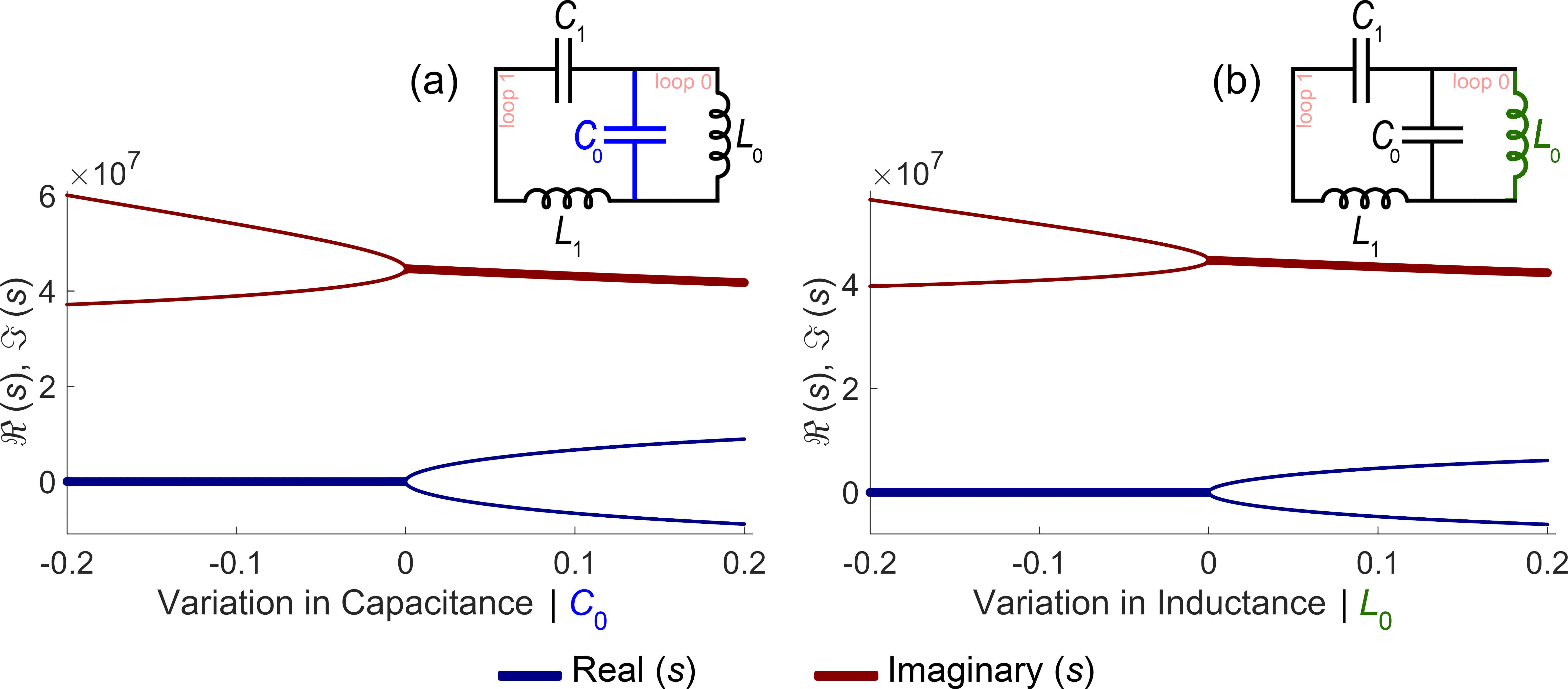
Figure 1. The real (dark blue solid curve) and imaginary (dark red solid curve) parts of the eigenvalues ($s=\mathrm{i}\omega$, where $\omega$ is eigenfrequency) of the circuit by varying (a) capacitance ($C_{0}$) and (b) inductance ($L_{0})$. In these plots, thicker lines indicate a multiplicity of two, and we limited the plots to eigenvalues with positive imaginary parts. Due to the bifurcation near the EPD, a second-order EPD with high sensitivity can be applied to sensing applications. Also, the proposed reciprocal circuit is shown here where the perturbed elements are colored in blue (capacitor) and green (inductor).

In this paper, we advance a perfectly conservative and reciprocal circuit that can be used to obtain the desired Jordan canonical form and achieve second-order EPD. Our comparative studies of reciprocal and nonreciprocal circuits suggest that circuit reciprocity information is not necessarily encoded in the relevant Jordan canonical form but rather in certain symmetries of the system eigenvectors. In addition, both reciprocal and nonreciprocal schemes can lead to the same eigenvalues whereas their Lagrangian equations are different. We demonstrate the conditions for equivalence between reciprocal and nonreciprocal circuits in general (i.e., when circuits are degenerate or non-degenerate) to have the same Jordan canonical form despite different Lagrangian equations. The present study includes mathematical analysis as well as extensive time-domain numerical simulation results for verification that were computed by a well-known commercial circuit simulator. The eigenvalues of the proposed circuit, which will be discussed later, are exceedingly sensitive to perturbations in circuit parameters (such as capacitance or inductance) as shown in Figure 1. Hence, the proposed circuit provides exceptional capabilities for applications that require high-sensitivity sensing when a component of the circuit, which is essentially a sensing component, is perturbed externally.

The structure of the paper is as follows. The mathematical setup of the problem is presented in Section 2. The main achievements and results of this paper are summarized in Section 3. Then, we demonstrate our primary circuit with lossless and reciprocal elements in Section 4. We study the Jordan canonical form of the circuit and the condition to obtain second-order EPD in our proposed circuit in Section 5. Section 6 demonstrates the Lagrangian and Hamiltonian structures and their relation in the general case. Next, we review briefly the gyrator-based circuit introduced in our previous studies and explain the mathematical analysis behind the nonreciprocal design in Section 7. In Section 8, we analyze both reciprocal and nonreciprocal circuits to identify the signs of nonreciprocity in the Lagrangian equations and eigenvectors of the circuits. Also, we provide the equivalency condition for both reciprocal and nonreciprocal circuits in Section 9 to have the same eigenvalues while the circuits’ Lagrangian equations are different. Finally, we support our mathematical analysis and findings by giving examples that are verified by using a time-domain circuit simulator in Section 10 and wrapping up the paper in Section 11. Also, we include many appendices for readers to provide more information and details.

2. Mathematical Setup of The Problem

Our primary goal here is to develop a lossless electric circuit with $2$ fundamental loops (see circuit in Figure 1) so that its evolution matrix $\mathscr{H}$ has a prescribed Jordan canonical form $\mathscr{J}$ subject to natural constraints considered later on. According to the definition of the Jordan canonical form, we have $\mathscr{H}=\mathscr{S}\mathscr{J}\mathscr{S}^{-1}$ where $\mathscr{S}$ is an invertible $4\times 4$ matrix for the two-loop circuit that is a block diagonal matrix of the form

$$\mathscr{J}=\left[\begin{array}[]{cc}J\left(\zeta_{1}\right)&0_{2}\\ 0_{2}&J\left(\zeta_{2}\right)\end{array}\right],\quad J\left(\zeta_{j}\right)=\left[\begin{array}[]{cc}\zeta_{j}&1\\ 0&\zeta_{j}\end{array}\right],\quad j=1,2,$$ (2.5)

where $0_{2}$ is $2\times 2$ zero matrix, $\zeta_{j}$ are real or complex numbers, and $J\left(\zeta_{j}\right)$ are the corresponding so-called Jordan block. As to the evolution circuit matrix $\mathscr{H}$ we assume that the circuit evolution is governed by the following Hamilton evolution equation

$$\partial_{t}\mathscr{X}=\mathscr{H}\mathscr{X},$$ (2.6)

where $\mathscr{X}$ is $4$ dimensional vector-column describing the circuit state and $\mathscr{H}$ is $4\times 4$ matrix. The matrix $\mathscr{H}$ is going to be a Hamiltonian matrix and we will refer to it as the circuit evolution matrix or just circuit matrix (see Section 6). Also, the circuit state vector is described by the corresponding two time dependent charges $q_{j}\left(t\right)$ ($j=1,2$) which are the time integrals of the relevant loop currents $\partial_{t}q_{k}\left(t\right)$ (see the circuits in Figure 1).

The eigenvalue problem of Equation (2.6) can be written as

$$s\mathscr{X}=\mathscr{H}\mathscr{X},\quad s=\mathrm{i}\omega,$$ (2.7)

where $s$ is the eigenvalue and $\omega$ is the eigenfrequency. It turns out that if the Jordan canonical form $\mathscr{J}$ of the circuit matrix $\mathscr{H}$ has a nontrivial Jordan block then the circuit must have at least one negative capacitance and inductance (see Section 5.1). The origin of the constraints is the fundamental property of a Hamiltonian matrix $\mathscr{H}$ to be similar to $-\mathscr{H}^{\mathrm{T}}$ where $\mathscr{H}^{\mathrm{T}}$ is the transposed to $\mathscr{H}$ matrix. Apart from the Hamiltonian spectral symmetry the Jordan structure of Hamiltonian matrices can be arbitrary. Our approach to the generation of Hamiltonian and the corresponding Hamiltonian matrices is intimately related to the Hamiltonian canonical forms (see Appendix F of [25]).

Another significant mathematical input to the synthesis of the simplest possible systems exhibiting nontrivial Jordan blocks comes from the property of a square matrix $\mathscr{M}$ to be cyclic (also called non-derogatory) (see Appendix B of [25]). We remind that a square matrix $\mathscr{M}$ is called cyclic if the geometric multiplicity of each of its eigenvalues is exactly $1$. It means that every eigenvalue of matrix $\mathscr{M}$ has exactly one eigenvector. Consequently, if a square matrix $\mathscr{M}$ is cyclic its Jordan form $\mathscr{J}_{\mathscr{M}}$ is completely determined by its characteristic polynomial $\chi\left(s\right)=\det\left\{s\mathbb{I}_{4}-\mathscr{M}\right\}$ where $\mathbb{I}_{4}$ is the $4\times 4$ identity matrix. Namely, every eigenvalue $s_{0}$ of $\mathscr{M}$ of multiplicity $2$ is associated with the single Jordan block $J\left(s_{0}\right)$ in the Jordan form $\mathscr{J}_{\mathscr{M}}$ of $\mathscr{M}$. Consequently, for a cyclic matrix $\mathscr{M}$ its characteristic polynomial encodes all the information about its Jordan form $\mathscr{J}_{\mathscr{M}}$. Another property of any cyclic matrix $\mathscr{M}$ associated with the a monic polynomial $\chi$ is that it is similar to the so-called companion matrix $C_{\chi}$ defined by simple explicit expression involving the coefficients of the polynomial $\chi$ (see Appendix B of [25]).

Companion matrix $C_{\chi}$ is naturally related to the high-order differential equation $\chi\left(\partial_{t}\right)x\left(t\right)=0$, where $x\left(t\right)$ is a complex-valued function of $t$ (see Appendices B and D of [25]). This fact underlines the relevance of the cyclicity property to the evolution of simpler systems described by higher order differential equations for a scalar function. Accordingly, we focus on cyclic Hamiltonian matrices $\mathscr{H}$ for they lead to the simplest circuits with the evolution matrices $\mathscr{H}$ having nontrivial Jordan forms $\mathscr{J}$.

Suppose the prescribed Jordan form $\mathscr{J}$ is an $4$$\times 4$ matrix subject to the Hamiltonian spectral symmetry and the cyclicity conditions. For this circuit we have the characteristic polynomial $\chi\left(s\right)=\det\left\{s\mathbb{I}_{4}-\mathscr{J}\right\}$ which is an even monic polynomial $\chi\left(s\right)$ of the degree 4. We consider then the companion to $\chi\left(s\right)$ matrix $\mathscr{C}$ (see Appendix B of [25]), that is

$$\mathscr{C}=\mathscr{Y}\mathscr{J}\mathscr{Y}^{-1},$$ (2.8)

where the columns of matrix $\mathscr{Y}$ form the so-called Jordan basis of the companion matrix $\mathscr{C}$ associated with the characteristic polynomial $\chi\left(s\right)=\det\left\{s\mathbb{I}_{4}-\mathscr{J}\right\}$. We proceed with an introduction of our principal Hamiltonian $\mathcal{H}$ and recover from it $4\times 4$ Hamiltonian matrix $\mathscr{H}$ that governs the system evolution according to Equation (2.6). As the result of our particular choice of the Hamiltonian $\mathcal{H}$ the corresponding to it Hamiltonian matrix $\mathscr{H}$ is similar to the companion matrix $\mathscr{C}$ and consequently it has exactly the same Jordan form $\mathscr{J}$ as $\mathscr{C}$. In particular, we construct an $4\times 4$ matrix $\mathscr{T}$ such that

$$\mathscr{C}=\mathscr{T}^{-1}\mathscr{H}\mathscr{T},\quad\mathscr{H}=\mathscr{Z}\mathscr{J}\mathscr{Z}^{-1},\quad\mathscr{Z}=\mathscr{T}\mathscr{Y},$$ (2.9)

where the columns of matrix $\mathscr{Z}$ form a Jordan basis of the evolution matrix $\mathscr{H}$. The Equations (2.8) and (2.9) between involved matrices are considered in Section 6.

3. Review of The Main Results

We advance here a perfectly conservative circuit without a gyrator which has an EPD and consequently a nontrivial Jordan canonical form. This circuit is shown in Figure 2(a) and we will refer to it as a principle reciprocal circuit (PRC) or simply a reciprocal circuit in the rest of the paper. The circuit has only four elements which are all lossless and reciprocal. The nontrivial Jordan canonical form is already obtained in the gyrator-based nonreciprocal circuit (GNC) which has a nonreciprocal element [25, 26, 27, 30, 29], as shown in Figure 2(b). The list of components for reciprocal and nonreciprocal circuits and the necessary conditions to pick the equivalency value of gyration resistance is summarized in Table 1. The list of our main achievements that are elaborated in the rest of the paper is as follows:

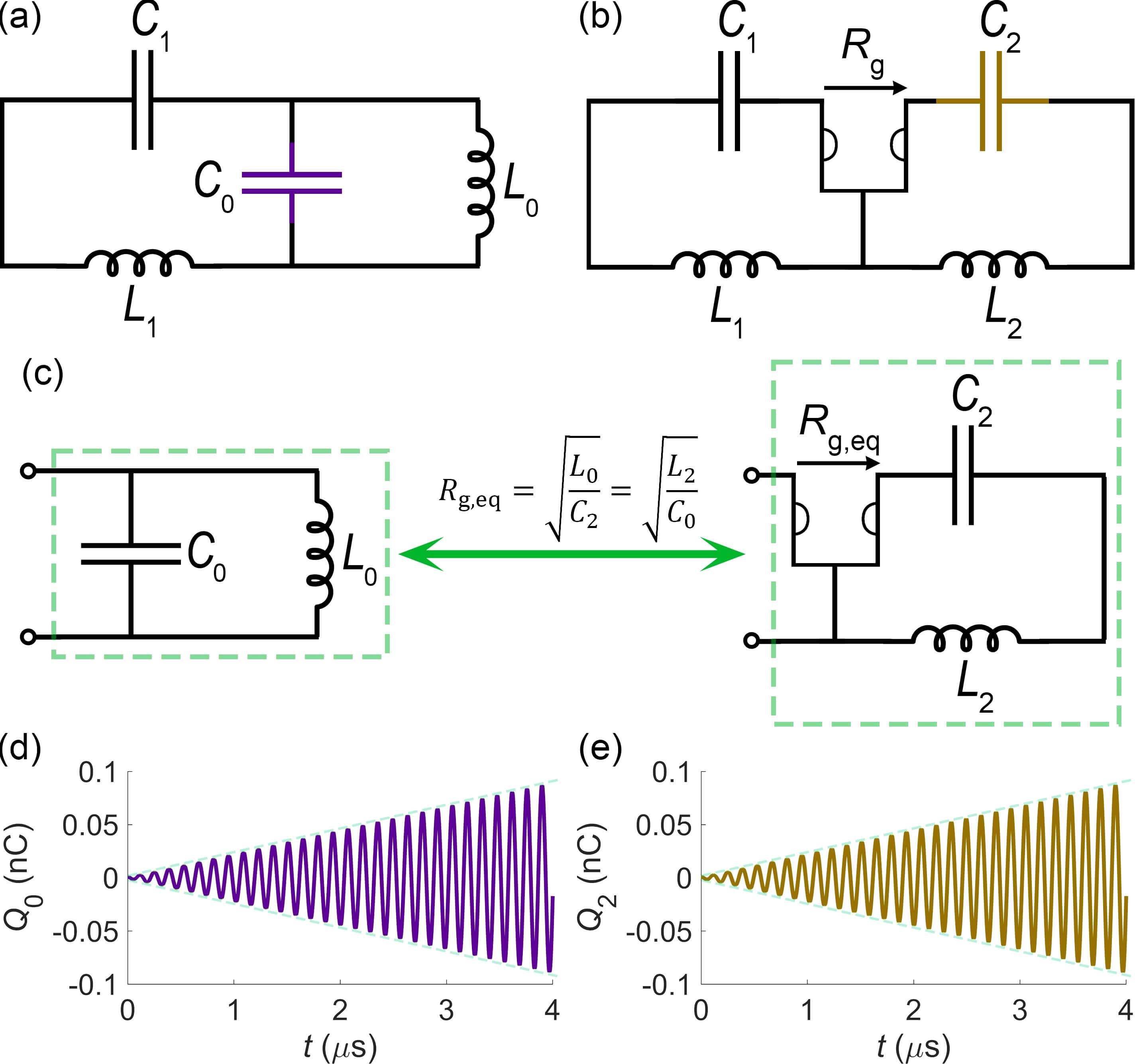
Figure 2. Comparison between (a) the 4-element reciprocal circuit (the focus of this paper), also denoted as PRC, and (b) the 5-element nonreciprocal circuit that uses a gyrator as a nonreciprocal element, also denoted as GNC. (c) Equivalent resonators with the equivalency value of gyration resistance $R_{\mathrm{g,eq}}=\sqrt{L_{0}/C_{2}}=\sqrt{L_{2}/C_{0}}$. Stored charges calculated by time-domain circuit simulator in (d) the capacitor of the PRC $C_{0}$ and (e) the capacitor of the GNC $C_{2}\left(t\right)$ under the both EPD and equivalency conditions. Furthermore, the envelope of the charge signals shows linear growth over time, which is a distinguishing characteristic of second-order EPDs.

• Construction of a reciprocal and lossless circuit with an EPD. We prove that the nontrivial Jordan canonical form can be obtained in a circuit without gyrator (see Section 4).

• PRC can have exactly the same Jordan canonical form as GNC and we find conditions for this to occur. If we consider the gyration resistance value of $R_{\mathrm{g,eq}}$ (see Figure 2(c)), the reciprocal and nonreciprocal circuits can have the same Jordan canonical forms implying that the eigenvalues of both circuits are the same. We conducted extensive numerical simulations of PRC and GNC using a commercial time-domain circuit simulator for comparison. In particular, we observe the charge stored in the capacitor associated with right loops as shown in Figures 2(d) and (e) for reciprocal ($C_{0}$) and nonreciprocal ($C_{2}$) circuits, respectively. There is excellent agreement between numerical simulations and the above condition of equivalency is satisfied as demonstrated by numerical simulations (see Sections 10 and 9).

• Our analysis of the spectral data shows that nonreciprocity in the GNC is manifested in the breakdown of certain symmetries for the set of eigenvectors while this symmetry exists for PRC. The nonreciprocity is also manifested in the circuit Lagrangian. Despite this, nonreciprocity is not captured by analyzing the eigenvalues or the Jordan canonical form of the circuit matrix (see Section 8).

Table 1. List of component and required conditions for equivalent reciprocal and nonreciprocal circuits.

	4-Element⋆	5-Element†	Equivalency
Capacitance - first loop	$C_{1}$	$C_{1}$
Inductance - first loop	$L_{1}$	$L_{1}$	$L_{1}C_{1}=L_{1}C_{1}$
Capacitance - second loop	$C_{0}$	$C_{2}$
Inductance - second loop	$L_{0}$	$L_{2}$	$L_{2}C_{2}=L_{0}C_{0}$
Gyrator	None	$R_{g}$	$R_{\mathrm{g,eq}}=\sqrt{\frac{L_{0}}{C_{2}}}=\sqrt{\frac{L_{2}}{C_{0}}}$

$\qquad{}^{\star}$ 4-Element: Principal reciprocal circuit (PRC)

$\qquad{}^{\dagger}$ 5-Element: Gyrator-based nonreciprocal circuit (GNC)

4. Principal Reciprocal Circuit (PRC)

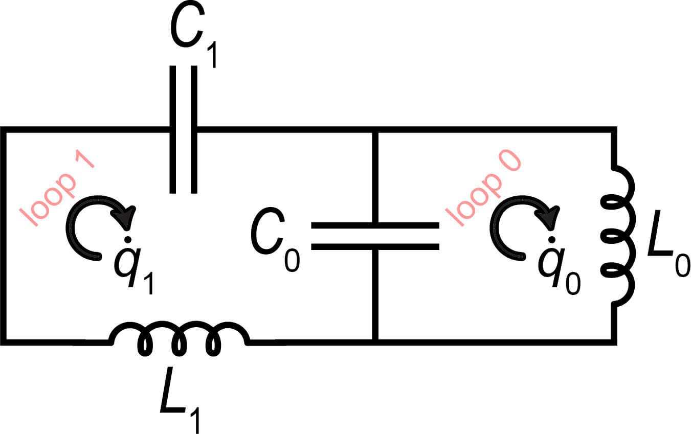
Figure 3. The principal two-loop circuit with reciprocal and lossless elements. For particular choices of values for quantities $L_{1}$, $C_{1}$, $L_{0}$, and $C_{0}$, the evolution matrix of the circuit develops second-order degeneracy, and its nontrivial Jordan canonical form consists of exactly two Jordan blocks of size 2. In this circuit, it is possible to replace $C_{0}$ and $L_{0}$ with each other since they are parallel. It is noteworthy that the zeroth loop and the first loop serve different purposes, with the capacitance $C_{0}$ being shared within the loops to couple them together.

We advance here our proposed simple reciprocal circuit with a circuit matrix having the nontrivial Jordan canonical form without the need for gyrator. Figure 3 shows the PRC made of two fundamental loops connected directly. In this circuit, quantities $L_{j}$ and $C_{j}$ ($j=0,1$) are respectively inductance and capacitance of the corresponding loops. The Lagrangian associated with PRC displayed in Figure 3 is expressed by

$$\left.\mathcal{L}_{\mathrm{r}}\left(\mathrm{q}_{\mathrm{r}},\partial_{t}\mathrm{q}_{\mathrm{r}}\right)\right|_{\Theta_{\mathrm{r}}}=\frac{L_{1}\left(\partial_{t}q_{1}\right)^{2}}{2}+\frac{L_{0}\left(\partial_{t}q_{0}\right)^{2}}{2}-\frac{\left(q_{1}\right)^{2}}{2C_{1}}-\frac{\left(q_{1}-q_{0}\right)^{2}}{2C_{0}},$$ (4.1a)

$$q_{j}\left(t\right)=\int^{t}i_{j}\left(t^{\prime}\right)\,\mathrm{d}t^{\prime},\quad j=0,1,$$ (4.1b)

where $q_{j}$ and $i_{j}$ are the charges and the currents associated with loops of the PRC depicted in Figure 3 and $\Theta_{\mathrm{r}}=\left\{L_{1},L_{0},C_{1},C_{0}\right\}$ is the set of circuit’s parameters. We introduce a vector of charges as $\mathrm{q}_{\mathrm{r}}=\left[q_{1},q_{0}\right]^{\mathrm{T}}$ ($\mathrm{T}$ denotes the transpose operator) that composed of the charges associated with two fundamental loops. According to time reversal symmetry in reciprocal systems, the Lagrangian associated with the PRC depicted in Figure 3 has the property $\mathcal{L}_{\mathrm{r}}\left(\mathrm{q}_{\mathrm{r}},\partial_{t}\mathrm{q}_{\mathrm{r}}\right)=\mathcal{L}_{\mathrm{r}}\left(\mathrm{q}_{\mathrm{r}},-\partial_{t}\mathrm{q}_{\mathrm{r}}\right)$. The reciprocity principle and features of the Lagrangian formulations will be further examined in Subsection 8.1. The corresponding Euler-Lagrange equations of the PRC are given by

$$\frac{d}{dt}\left(\frac{\partial}{\partial\dot{q}_{1}}\mathcal{L}\right)-\frac{\partial}{\partial q_{1}}\mathcal{L}=0,$$ (4.2a)

$$\frac{d}{dt}\left(\frac{\partial}{\partial\dot{q}_{0}}\mathcal{L}\right)-\frac{\partial}{\partial q_{0}}\mathcal{L}=0,$$ (4.2b)

which are simplified in the form of

$$L_{1}\ddot{q}_{1}+\left(\frac{1}{C_{1}}+\frac{1}{C_{0}}\right)q_{1}-\frac{1}{C_{0}}q_{0}=0,$$ (4.3a)

$$L_{0}\ddot{q}_{0}-\frac{1}{C_{0}}q_{1}+\frac{1}{C_{0}}q_{0}=0.$$ (4.3b)

It is well known that the Euler-Lagrange formulations of Equations (4.3a) and (4.3b) represent the Kirchhoff voltage law for each of the two fundamental loops. The Kirchhoff voltage equations for the PRC are calculated in Appendix A. Accordingly, each term in Equations (4.3a) and (4.3b) corresponds to the voltage drop of the relevant element, as can be seen from the current-voltage relations reviewed in Appendix B.1.

The circuit vector evolution equation by using the state vector of $\mathsf{q}_{\mathrm{r}}=\left[\mathrm{q}_{\mathrm{r}},\partial_{t}\mathrm{q}_{\mathrm{r}}\right]^{\mathrm{T}}$ is given by

$$\partial_{t}\mathsf{q}_{\mathrm{r}}=\mathscr{C}_{\mathrm{r}}\mathsf{q}_{\mathrm{r}},\quad\mathscr{C}_{\mathrm{r}}=\left[\begin{array}[]{rrcr}0&0&1&0\\ 0&0&0&1\\ -\left(\frac{1}{L_{1}C_{1}}+\frac{1}{L_{1}C_{0}}\right)&\frac{1}{L_{1}C_{0}}&0&0\\ \frac{1}{L_{0}C_{0}}&-\frac{1}{L_{0}C_{0}}&0&0\end{array}\right],$$ (4.4)

where $\mathscr{C}_{\mathrm{r}}$ is circuit matrix corresponding to the PRC. The characteristic polynomial related to the matrix $\mathscr{C}_{\mathrm{r}}$ defined by Equation (4.4) is expressed by

$$\chi_{\mathrm{r}}\left(s\right)=\det\left\{s\mathbb{I}_{4}-\mathscr{C}_{\mathrm{r}}\right\}=s^{4}+s^{2}\left(\xi_{1}+\xi_{0}+\delta\right)+\xi_{1}\xi_{0}=0,$$ (4.5)

where $\mathbb{I}_{4}$ is the $4\times 4$ identity matrix and the circuit resonance frequencies are defined as

$$\delta=\frac{1}{L_{1}C_{0}},\quad\xi_{0}=\frac{1}{L_{0}C_{0}},\quad\xi_{1}=\frac{1}{L_{1}C_{1}}.$$ (4.6)

In the above equations, $\sqrt{\zeta_{0}}$ indicates the resonance frequency of the zeroth loop, $\sqrt{\zeta_{1}}$ indicates the resonance frequency of the first loop and $\sqrt{\delta}$ is defined as a cross loop resonance frequency or coupling term. We demonstrate the following properties in the structure of the characteristic polynomial: (i) the characteristic polynomial is a quadratic equation in $s^{2}$, so if $s$ is the solution of the characteristic polynomial then $-s$ is its solution as well; (ii) the coefficients of the characteristic polynomial are real; hence $s$ and $s^{*}$ (^∗ denotes the complex conjugate operation) are both solutions of the characteristic polynomial. Note that using circuit resonance frequencies defined in Equation (4.6), we recast the circuit matrix $\mathscr{C}_{\mathrm{r}}$ in Equation (4.4) as below

$$\mathscr{C}_{\mathrm{r}}=\left[\begin{array}[]{rrcr}0&0&1&0\\ 0&0&0&1\\ -\xi_{1}-\delta&\delta&0&0\\ \xi_{0}&-\xi_{0}&0&0\end{array}\right],$$ (4.7)

which shows that matrix $\mathscr{C}_{\mathrm{r}}$ defined by Equation (4.7) is a block off-diagonal matrix.

5. The Jordan Canonical Form of PRC

We studied the PRC composed of two loops, as shown in Figure 3, without putting any constraints on the circuit parameters $L_{1}$, $C_{1}$, $L_{0}$, and $C_{0}$ except that they are all real and non-zero. In this section, we derive the most general conditions on the circuit parameters under which the relevant evolution matrix shows nontrivial Jordan blocks. The Lagrangian equation for the PRC is given by Equation (4.1a), and its evolution equations are the corresponding Euler-Lagrange equations:

$$s^{2}q_{1}+\left(\xi_{1}+\delta\right)q_{1}-\delta q_{0}=0,$$ (5.1a)

$$s^{2}q_{0}-\xi_{0}q_{1}+\xi_{0}q_{0}=0.$$ (5.1b)

The Euler-Lagrange equations are readily recast in the below matrix form,

$$\mathrm{A}_{\mathrm{r}}\left(s\right)\mathrm{q}_{\mathrm{r}}=0,\quad\mathrm{A}_{\mathrm{r}}\left(s\right)=\left[\begin{array}[]{rr}s^{2}+\xi_{1}+\delta&-\delta\\ -\xi_{0}&s^{2}+\xi_{0}\end{array}\right],$$ (5.2)

where $\mathrm{A}_{\mathrm{r}}\left(s\right)$ is a $2\times 2$ monic matrix polynomial of $s$ of degree 2, namely,

$$\mathrm{A}_{\mathrm{r}}\left(s\right)=\sum_{j=0}^{2}s^{j}\mathrm{A}_{\mathrm{r},j}=s^{2}\mathrm{A}_{\mathrm{r},2}+s\mathrm{A}_{\mathrm{r},1}+\mathrm{A}_{\mathrm{r},0},$$ (5.3a)

$$\mathrm{A}_{\mathrm{r},2}=\left[\begin{array}[]{rr}1&0\\ 0&1\end{array}\right],\quad\mathrm{A}_{\mathrm{r},1}=\left[\begin{array}[]{rr}0&0\\ 0&0\end{array}\right],\quad\mathrm{A}_{\mathrm{r},0}=\left[\begin{array}[]{rr}\xi_{1}+\delta&-\delta\\ -\xi_{0}&\xi_{0}\end{array}\right].$$ (5.3b)

Then, Equation (5.2) is reduced to the standard first-order vector differential equation

$$s\mathsf{q}_{\mathrm{r,s}}=\mathscr{C}_{\mathrm{r}}\mathsf{q}_{\mathrm{r,s}},\quad\mathsf{q}_{\mathrm{r,s}}=\left[\begin{array}[]{r}\mathrm{q}_{\mathrm{r}}\\ s\mathrm{q}_{\mathrm{r}}\end{array}\right],\quad\mathscr{C}_{\mathrm{r}}=\left[\begin{array}[]{rrcr}0&0&1&0\\ 0&0&0&1\\ -\xi_{1}-\delta&\delta&0&0\\ \xi_{0}&-\xi_{0}&0&0\end{array}\right],$$ (5.4)

where $\mathscr{C}_{\mathrm{r}}$ is the $4\times 4$ companion matrix for the matrix polynomial $\mathrm{A}_{\mathrm{r}}\left(s\right)$. The standard eigenvalue problem is expressed as

$$\left(s\mathbb{I}_{4}-\mathscr{C}_{\mathrm{r}}\right)\mathsf{q}_{\mathrm{r,s}}=0.$$ (5.5)

Then, the characteristic polynomial of the matrix polynomial $\mathrm{A}_{\mathrm{r}}\left(s\right)$ is

$$\chi_{\mathrm{r}}\left(s\right)=\det\left\{\mathrm{A}_{\mathrm{r}}\left(s\right)\right\}=s^{4}+s^{2}\left(\xi_{1}+\xi_{0}+\delta\right)+\xi_{1}\xi_{0}.$$ (5.6)

Consequently, the characteristic polynomial $\chi_{\mathrm{r}}\left(s\right)=0$ can be used to calculate the eigenvalues associated with Equation (5.5). We aim in this paper to find all non-zero and real values of the circuit parameters $L_{1}$, $C_{1}$, $L_{0}$ and $C_{0}$ that lead to the matrix $\mathscr{C}_{\mathrm{r}}$ defined by Equation (5.4) having a nontrivial Jordan canonical form.

5.1. Characteristic polynomial and eigenvalue degeneracy

We present here the condition for degenerate eigenvalues in the characteristic polynomial. We rewrite the characteristic polynomial associated with the PRC matrix as

$$\chi_{\mathrm{r}}\left(h\right)=h^{2}+h\left(\xi_{1}+\xi_{0}+\delta\right)+\xi_{1}\xi_{0}=0,\quad h=s^{2}.$$ (5.7)

A quadratic equation in $h$, $\chi_{\mathrm{r}}\left(h\right)=0$, has exactly two solutions, viz,

$$h_{\pm}=\frac{-\left(\xi_{1}+\xi_{0}+\delta\right)\pm\sqrt{\Delta_{\mathrm{r},h}}}{2},$$ (5.8)

where $\Delta_{\mathrm{r},h}=\delta^{2}+2\delta\left(\xi_{1}+\xi_{0}\right)+\left(\xi_{1}-\xi_{0}\right)^{2}$ is the discriminant of the quadratic in the characteristic polynomial of Equation (5.7). The four solutions of the characteristic polynomial $\chi_{\mathrm{r}}\left(s\right)=0$ are as follows:

$$s=\pm\sqrt{h_{+}},\pm\sqrt{h_{-}}.$$ (5.9)

Note that the eigenvalue degeneracy condition turns into $\Delta_{\mathrm{r},h}=0$, which is equivalently expressed as

$$\delta^{2}+2\delta\left(\xi_{1}+\xi_{0}\right)+\left(\xi_{1}-\xi_{0}\right)^{2}=0.$$ (5.10)

Equation (5.10) is a quadratic equation which has exactly two solutions. We refer to solutions of $\delta$ in Equation (5.10) as special values of degeneracy $\delta_{\mathrm{d,\pm}}$, where these two solutions are

$$\delta_{\mathrm{d,\pm}}=-\xi_{1}-\xi_{0}\pm 2\sqrt{\xi_{1}\xi_{0}}.$$ (5.11)

For the two special values of degeneracy $\delta_{\mathrm{d,\pm}}$ we get from Equation (5.8) the corresponding two degenerate roots of $h$ are given by

$$h_{\mathrm{d,}\pm}=-\frac{\xi_{1}+\xi_{0}+\delta_{\mathrm{d,\pm}}}{2}=\mp\sqrt{\xi_{1}\xi_{0}}.$$ (5.12)

The expression of Equation (5.11) is real-valued if and only if $\xi_{1}\xi_{0}>0$, or equivalently

$$\mathrm{\frac{\xi_{0}}{\left|\xi_{0}\right|}=\frac{\xi_{1}}{\left|\xi_{1}\right|}=\pm 1.}$$ (5.13)

Equation (5.13) implies that the equality of resonance frequencies sign, $\mathrm{sign}\left(\xi_{0}\right)=\mathrm{sign}\left(\xi_{1}\right)$, is a necessary condition for the eigenvalue degeneracy condition $\Delta_{\mathrm{r},h}=0$ provided that $\delta_{\mathrm{d,\pm}}$ has to be real-valued. From Equations (5.11) and (5.13), it follows that the special values of degeneracy $\delta_{\mathrm{d,\pm}}$ can be expressed as $\delta_{\mathrm{d,\pm}}=-\left(\sqrt{\xi_{1}}\mp\sqrt{\xi_{0}}\right)^{2}$.

Theorem 1 (Nontrivial Jordan canonical form of the companion matrix).

Let’s assume that $s_{0}$ is an eigenvalue of the companion matrix $\mathscr{C}_{\mathrm{r}}$ given in Equation (5.4) such that its algebraic multiplicity $m\left(s_{0}\right)$$=2$. Then (i) $s_{0}\neq 0$; (ii) $s_{0}$ is either purely real or purely imaginary; (iii) $-s_{0}$ is also an eigenvalue of the companion matrix $\mathscr{C}_{\mathrm{r}}$; (iv) $m\left(s_{0}\right)$$=m\left(-s_{0}\right)=2$; and (v) the nontrivial Jordan canonical form of the companion matrix $\mathscr{C}_{\mathrm{r}}$ is expressed as

$$\mathscr{\mathscr{J}}_{\mathrm{r}}=\left[\begin{array}[]{rrrr}s_{0}&1&0&0\\ 0&s_{0}&0&0\\ 0&0&-s_{0}&1\\ 0&0&0&-s_{0}\end{array}\right].$$ (5.14)

It follows that the eigenvalue degeneracy for the companion matrix $\mathscr{C}_{\mathrm{r}}$ implies that its Jordan canonical form $\mathscr{\mathscr{J}}_{\mathrm{r}}$ has two Jordan blocks of size 2. A proof of this theorem can be found in [25].

5.2. Eigenvectors and the Jordan basis

Theorem 1 states that the degeneracy of eigenvalues in the companion matrix $\mathscr{C}_{\mathrm{r}}$ given by Equation (5.4) implies that its Jordan canonical form consists of two Jordan blocks as in Equation (5.14). The Jordan canonical form corresponding to the companion matrix $\mathscr{C}_{\mathrm{r}}$ in the non-degenerate form, $\Delta_{\mathrm{r},h}\neq 0$, is expressed as

$$\mathscr{J}_{\mathrm{r}}=\left[\begin{array}[]{rrrr}\mathrm{i}s_{1}&0&0&0\\ 0&-\mathrm{i}s_{1}&0&0\\ 0&0&\mathrm{i}s_{2}&0\\ 0&0&0&-\mathrm{i}s_{2}\end{array}\right],\quad\begin{array}[]{c}s_{1}=\sqrt{\frac{\xi_{\mathrm{s}}+\sqrt{\Delta_{\mathrm{r},h}}}{2}}\\ s_{2}=\sqrt{\frac{\xi_{\mathrm{s}}-\sqrt{\Delta_{\mathrm{r},h}}}{2}}\end{array},\quad\xi_{\mathrm{s}}=\xi_{1}+\xi_{0}+\delta,$$ (5.15)

where $\xi_{\mathrm{s}}$ is the sum of three resonance frequencies square defined in Equation (4.6), $\Delta_{\mathrm{r},h}$ is the discriminant of the quadratic equation defined after Equation (5.8) and $\pm\mathrm{i}s_{i}$ ($i=1,2$) are the corresponding eigenvalues. Following this, we write eigenvectors corresponding to the calculated non-degenerate eigenvalues as follows:

$$\mathscr{V}_{\mathrm{r}}=\left[\mathsf{e}_{\mathrm{r},+s_{1}}|\mathsf{e}_{\mathrm{r},-s_{1}}|\mathsf{e}_{\mathrm{r},+s_{2}}|\mathsf{e}_{\mathrm{r},-s_{2}}\right],$$ (5.16a)

$$\begin{array}[]{c}\mathsf{e}_{\mathrm{r},\pm s_{i}}=\left[\begin{array}[]{r}\mp\frac{\left(-s_{i}^{2}\right)^{3/2}+\left(\xi_{0}+\delta\right)\sqrt{-s_{i}^{2}}}{\xi_{1}\xi_{0}}\\ \mp\frac{\left(-s_{i}^{2}\right)^{3/2}+\xi_{\mathrm{s}}\sqrt{-s_{i}^{2}}}{\xi_{1}\xi_{0}}\\ 1-\frac{s_{i}^{2}}{\xi_{0}}\\ 1\end{array}\right].\end{array}$$ (5.16b)

Next, we investigate two different cases with two special values of degeneracy $\delta_{\mathrm{d,\pm}}$, which lead to degeneracy with purely imaginary or purely real degenerate eigenvalues.

5.2.1. Degeneracy with purely imaginary eigenvalues (purely real eigenfrequencies)

In the first case, if we consider $\delta=\delta_{\mathrm{d},+}=-\xi_{1}-\xi_{0}+2\sqrt{\xi_{1}\xi_{0}}$, the characteristic polynomial is rewritten as

$$\chi_{\mathrm{r},+}\left(s\right)=s^{4}+2s^{2}\sqrt{\xi_{1}\xi_{0}}+\xi_{1}\xi_{0}=\left(s^{2}+\sqrt{\xi_{1}\xi_{0}}\right)^{2}=0.$$ (5.17)

Then, the degenerate companion matrix $\mathscr{C}_{\mathrm{r},+}$ for this degenerate case is given by

$$\mathscr{C}_{\mathrm{r},+}=\left[\begin{array}[]{rrrr}0&0&1&0\\ 0&0&0&1\\ -\delta_{\mathrm{d},+}-\xi_{1}&\delta_{\mathrm{d},+}&0&0\\ \xi_{0}&-\xi_{0}&0&0\end{array}\right],$$ (5.18)

and the Jordan canonical form of the degenerate companion matrix $\mathscr{C}_{\mathrm{r},+}$ with purely imaginary eigenvalues (purely real eigenfrequencies) is expressed as

$$\mathscr{J}_{\mathrm{r},+}=\left[\begin{array}[]{rrrr}\mathrm{i}s_{\mathrm{e}}&1&0&0\\ 0&\mathrm{i}s_{\mathrm{e}}&0&0\\ 0&0&-\mathrm{i}s_{\mathrm{e}}&1\\ 0&0&0&-\mathrm{i}s_{\mathrm{e}}\end{array}\right],\quad s_{\mathrm{e}}=\left(\xi_{\mathrm{e}}\right)^{\frac{1}{2}}=\left(\xi_{0}\xi_{1}\right)^{\frac{1}{4}}.$$ (5.19)

As a result, the Jordan basis of the degenerate companion matrix $\mathscr{C}_{\mathrm{r},+}$ is obtained as follows:

$$\mathscr{Z}_{\mathrm{r},+}=\left[\begin{array}[]{rrrr}\frac{\xi_{0}-\xi_{\mathrm{e}}}{4\mathrm{i}\sqrt{\xi_{\mathrm{e}}}}&\frac{1}{2}&\frac{-\xi_{0}+\xi_{\mathrm{e}}}{4\mathrm{i}\sqrt{\xi_{\mathrm{e}}}}&\frac{1}{2}\\ \frac{\xi_{0}}{4\mathrm{i}\sqrt{\xi_{\mathrm{e}}}}&0&-\frac{\xi_{0}}{4\mathrm{i}\sqrt{\xi_{\mathrm{e}}}}&0\\ \frac{\xi_{0}\left(\xi_{\mathrm{e}}-\xi_{1}\right)}{4\xi_{\mathrm{e}}}&\frac{\xi_{0}\left(\xi_{\mathrm{e}}-3\xi_{1}\right)}{4\mathrm{i}\xi_{\mathrm{e}}\sqrt{\xi_{\mathrm{e}}}}&\frac{\xi_{0}\left(\xi_{\mathrm{e}}-\xi_{1}\right)}{4\xi_{\mathrm{e}}}&-\frac{\xi_{0}\left(\xi_{\mathrm{e}}-3\xi_{1}\right)}{4\mathrm{i}\xi_{\mathrm{e}}\sqrt{\xi_{\mathrm{e}}}}\\ -\frac{\xi_{0}^{2}\left(2\xi_{1}-\xi_{\mathrm{e}}\right)}{4\xi_{\mathrm{e}}\left(\xi_{0}-2\xi_{\mathrm{e}}\right)}&-\frac{\xi_{0}^{2}\left(2\xi_{1}-\xi_{\mathrm{e}}\right)}{4\mathrm{i}\xi_{\mathrm{e}}\sqrt{\xi_{\mathrm{e}}}\left(\xi_{0}-2\xi_{\mathrm{e}}\right)}&-\frac{\xi_{0}^{2}\left(2\xi_{1}-\xi_{\mathrm{e}}\right)}{4\xi_{\mathrm{e}}\left(\xi_{0}-2\xi_{\mathrm{e}}\right)}&\frac{\xi_{0}^{2}\left(2\xi_{1}-\xi_{\mathrm{e}}\right)}{4\mathrm{i}\xi_{e}\sqrt{\xi_{\mathrm{e}}}\left(\xi_{0}-2\xi_{\mathrm{e}}\right)}\end{array}\right].$$ (5.20)

Note that the columns of matrix $\mathscr{Z}_{\mathrm{r},+}$ form the Jordan bases of the corresponding degenerate companion matrix $\mathscr{C}_{\mathrm{r},+}$, and each column of $\mathscr{Z}_{\mathrm{r},+}$ are the generalized eigenvectors of the corresponding eigenvalues.

5.2.2. Degeneracy with purely real eigenvalues (purely imaginary eigenfrequencies)

In the second case, if we consider $\delta=\delta_{\mathrm{d},-}=-\xi_{1}-\xi_{0}-2\sqrt{\xi_{1}\xi_{0}}$, the characteristic polynomial is given by

$$\chi_{\mathrm{r},-}\left(s\right)=s^{4}-2s^{2}\sqrt{\xi_{1}\xi_{0}}+\xi_{1}\xi_{0}=\left(s^{2}-\sqrt{\xi_{1}\xi_{0}}\right)^{2}=0.$$ (5.21)

The corresponding degenerate companion matrix $\mathscr{C}_{\mathrm{r},-}$ is expressed by

$$\mathscr{C}_{\mathrm{r,-}}=\left[\begin{array}[]{rrrr}0&0&1&0\\ 0&0&0&1\\ -\delta_{\mathrm{d},-}-\xi_{1}&\delta_{\mathrm{d},-}&0&0\\ \xi_{0}&-\xi_{0}&0&0\end{array}\right].$$ (5.22)

Moreover, the Jordan canonical form of the corresponding degenerate companion matrix $\mathscr{C}_{\mathrm{r},-}$ in Equation (5.22) with purely real eigenvalues (purely imaginary eigenfrequencies) is written as

$$\mathscr{J}_{\mathrm{r,-}}=\left[\begin{array}[]{rrrr}s_{\mathrm{e}}&1&0&0\\ 0&s_{\mathrm{e}}&0&0\\ 0&0&-s_{\mathrm{e}}&1\\ 0&0&0&-s_{\mathrm{e}}\end{array}\right].$$ (5.23)

Then, the Jordan basis of the degenerate companion matrix $\mathscr{C}_{\mathrm{r,-}}$ is expressed as

$$\mathscr{Z}_{\mathrm{r,-}}=\left[\begin{array}[]{rrrr}\frac{\xi_{0}+\xi_{\mathrm{e}}}{4\sqrt{\xi_{\mathrm{e}}}}&\frac{1}{2}&-\frac{\xi_{0}+\xi_{\mathrm{e}}}{4\sqrt{\xi_{\mathrm{e}}}}&\frac{1}{2}\\ \frac{\xi_{0}}{4\sqrt{\xi_{\mathrm{e}}}}&0&-\frac{\xi_{0}}{4\sqrt{\xi_{\mathrm{e}}}}&0\\ \frac{\xi_{0}\left(\xi_{\mathrm{e}}+\xi_{1}\right)}{4\xi_{\mathrm{e}}}&\frac{\xi_{0}\left(\xi_{\mathrm{e}}+3\xi_{1}\right)}{4\xi_{\mathrm{e}}\sqrt{\xi_{\mathrm{e}}}}&\frac{\xi_{0}\left(\xi_{\mathrm{e}}+\xi_{1}\right)}{4\xi_{\mathrm{e}}}&-\frac{\xi_{0}\left(\xi_{\mathrm{e}}+3\xi_{1}\right)}{4\xi_{\mathrm{e}}\sqrt{\xi_{\mathrm{e}}}}\\ \frac{\xi_{0}^{2}\left(2\xi_{1}+\xi_{\mathrm{e}}\right)}{4\xi_{\mathrm{e}}\left(\xi_{0}+2\xi_{\mathrm{e}}\right)}&\frac{\xi_{0}^{2}\left(2\xi_{1}+\xi_{\mathrm{e}}\right)}{4\xi_{\mathrm{e}}\sqrt{\xi_{\mathrm{e}}}\left(\xi_{0}+2\xi_{\mathrm{e}}\right)}&\frac{\xi_{0}^{2}\left(2\xi_{1}+\xi_{\mathrm{e}}\right)}{4\xi_{\mathrm{e}}\left(\xi_{0}+2\xi_{\mathrm{e}}\right)}&-\frac{\xi_{0}^{2}\left(2\xi_{1}+\xi_{\mathrm{e}}\right)}{4\xi_{\mathrm{e}}\sqrt{\xi_{\mathrm{e}}}\left(\xi_{0}+2\xi_{\mathrm{e}}\right)}\end{array}\right].$$ (5.24)

6. Lagrangian and Hamiltonian Structures and Their Relation

In this section we provide a general overview of the Lagrangian and Hamiltonian structures. We explain the relationship between these two structures in detail. Then, we demonstrate the Lagrangian and Hamiltonian structures for the PRC. Ultimately, readers will gain a comprehensive understanding of these mathematical frameworks and their applicability to studying systems like the PRC.

6.1. Lagrangian structure

The Lagrangian for a linear system in the general form is a quadratic function (bilinear form) of the circuit state vector $\mathrm{\check{q}}$ (column vector that contains charges) and its time derivatives $\partial_{t}\mathrm{\check{q}}$, that is

$$\mathcal{L}=\mathcal{L}\left(\mathrm{\check{q}},\partial_{t}\mathrm{\check{q}}\right)=\frac{1}{2}\left[\begin{array}[]{r}\mathrm{\check{q}}\\ \partial_{t}\mathrm{\check{q}}\end{array}\right]^{\mathrm{T}}\mathrm{M}_{\mathrm{L}}\left[\begin{array}[]{r}\mathrm{\check{q}}\\ \partial_{t}\mathrm{\check{q}}\end{array}\right],\quad\mathrm{M}_{\mathrm{L}}=\left[\begin{array}[]{rr}-\eta&\theta^{\mathrm{T}}\\ \theta&\alpha\end{array}\right],$$ (6.7)

where $\alpha,\eta$ and $\theta$ are $2\times 2$ matrices (for our two-loops circuit) with real-valued entries. Moreover, we assume symmetric matrices, that is $\alpha=\alpha^{\mathrm{T}}$ and $\eta=\eta^{\mathrm{T}}$. Accordingly, we have the Lagrangian,

$$\mathcal{L}=\frac{1}{2}\partial_{t}\mathrm{\check{q}}^{\mathrm{T}}\alpha\partial_{t}\mathrm{\check{q}}+\partial_{t}\mathrm{\check{q}}^{\mathrm{T}}\theta\mathrm{\check{q}}-\frac{1}{2}\mathrm{\check{q}}^{\mathrm{T}}\eta\mathrm{\check{q}}.$$ (6.8)

As a result of Hamilton’s principle, the system evolution can be explained by the Euler-Lagrange equations as

$$\frac{d}{dt}\left(\frac{\partial\mathcal{L}}{\partial\dot{\mathrm{\check{q}}}}\right)-\frac{\partial\mathcal{L}}{\partial\mathrm{\check{q}}}=0,$$ (6.9)

which, based on Equation (6.8), it can be written in the following form of a second-order vector ordinary differential equation,

$$\alpha\partial_{t}^{2}\mathrm{\check{q}}+\left(\theta-\theta^{\mathrm{T}}\right)\partial_{t}\mathrm{\check{q}}+\eta\mathrm{\check{q}}=0.$$ (6.10)

It is notable that matrix $\theta$ appears in Equation (6.10) through its skew-symmetric component $\left(\theta-\theta^{\mathrm{T}}\right)/2$ justifying as a possibility to impose the skew-symmetry assumption on $\theta$, that is $\theta^{\mathrm{T}}=-\theta$. Then, under the assumption of $\theta^{\mathrm{T}}=-\theta$, Equation (6.10) is rewritten with the skew-symmetric $\theta$ as

$$\alpha\partial_{t}^{2}\mathrm{\check{q}}+2\theta\partial_{t}\mathrm{\check{q}}+\eta\mathrm{\check{q}}=0.$$ (6.11)

For the PRC that we introduced and analyzed in the previous sections, Equation (6.11) and the required coefficients by considering $\mathrm{\check{q}}=\mathrm{q}_{\mathrm{r}}=\left[q_{1},q_{0}\right]^{\mathrm{T}}$ are rewritten as

$$\alpha_{\mathrm{r}}\partial_{t}^{2}\mathrm{q}_{\mathrm{r}}+2\theta_{\mathrm{r}}\partial_{t}\mathrm{q}_{\mathrm{r}}+\eta_{\mathrm{r}}\mathrm{q}_{\mathrm{r}}=0,$$ (6.12a)

$$\alpha_{\mathrm{r}}=\left[\begin{array}[]{cc}L_{1}&0\\ 0&L_{0}\end{array}\right],\quad\theta_{\mathrm{r}}=\left[\begin{array}[]{cc}0&0\\ 0&0\end{array}\right],\quad\eta_{\mathrm{r}}=\left[\begin{array}[]{rr}\frac{1}{C_{1}}+\frac{1}{C_{0}}&-\frac{1}{C_{0}}\\ -\frac{1}{C_{0}}&\frac{1}{C_{0}}\end{array}\right].$$ (6.12b)

We write the Lagrangian equation in the below form:

$$\mathcal{L}_{\mathrm{r}}\left(\mathrm{q}_{\mathrm{r}},\partial_{t}\mathrm{q}_{\mathrm{r}}\right)=\frac{1}{2}\left[\begin{array}[]{r}\mathrm{q}_{\mathrm{r}}\\ \partial_{t}\mathrm{q}_{\mathrm{r}}\end{array}\right]^{\mathrm{T}}\mathrm{M}_{\mathrm{L,r}}\left[\begin{array}[]{r}\mathrm{q}_{\mathrm{r}}\\ \partial_{t}\mathrm{q}_{\mathrm{r}}\end{array}\right],$$ (6.13a)

$$\mathrm{M}_{\mathrm{L,r}}=\left[\begin{array}[]{rrrr}-\frac{1}{C_{1}}-\frac{1}{C_{0}}&\frac{1}{C_{0}}&0&0\\ \frac{1}{C_{0}}&-\frac{1}{C_{0}}&0&0\\ 0&0&L_{1}&0\\ 0&0&0&L_{0}\end{array}\right].$$ (6.13b)

It follows from Equation (6.10) that the necessary and sufficient condition for nonreciprocity is $\theta\neq\theta^{\mathrm{T}}$. Indeed, if $\theta=\theta^{\mathrm{T}}$, the circuit will not show nonreciprocity properties. Because in the case of $\theta=\theta^{\mathrm{T}}$, the second term with $\partial_{t}\mathrm{q}$ disappears from Equation (6.10) and all frequencies related to Equation (6.10) will be the same as in the case of zero $\theta$ which leads to time symmetry.

6.2. Hamiltonian

Alternatively, we can use the Hamilton equations associated with the Hamiltonian $\mathcal{H}$ instead of the second-order vector ordinary differential equations of Equation (6.10). Let us suppose that the system is described by a time-dependent column vector $\mathrm{\check{q}}$ and its dynamic is governed by a Hamiltonian $\mathcal{H}=\mathcal{H}\left(\mathrm{\check{p}},\mathrm{\check{q}}\right)$, where $\mathrm{\check{p}}$ is the column vector system momentum. We introduce the Hamiltonian representation in order to present the system information in compact matrix form,

$$\mathcal{H}=\mathcal{H}\left(\mathrm{\check{p}},\mathrm{\check{q}}\right)=\mathrm{\check{p}}^{\mathrm{T}}\partial_{t}\mathrm{\check{q}}-\mathcal{L}\left(\mathrm{\check{q}},\partial_{t}\mathrm{\check{q}}\right),$$ (6.14)

where the system momentum $\mathrm{\check{p}}$ is given by

$$\mathrm{\check{p}}=\frac{\partial\mathcal{L}}{\partial\dot{\mathrm{\check{q}}}}=\alpha\partial_{t}\mathrm{\check{q}}+\theta\mathrm{\check{q}}.$$ (6.15)

According to Equation (6.15), current $\partial_{t}\mathrm{\check{q}}$ (i.e., velocity of charges) and momentum $\mathrm{\check{p}}$ vectors are related as follows:

$$\partial_{t}\mathrm{\check{q}}=\alpha^{-1}\left(\mathrm{\check{p}}-\theta\mathrm{\check{q}}\right).$$ (6.16)

Consequently, the Hamiltonian $\mathcal{H}$ expressed in Equation (6.14) is given by

$$\mathcal{H}\left(\mathrm{\check{p}},\mathrm{\check{q}}\right)=\frac{1}{2}\left[\left(\mathrm{\check{p}}-\theta\mathrm{\check{q}}\right)^{\mathrm{T}}\alpha^{-1}\left(\mathrm{\check{p}}-\theta\mathrm{\check{q}}\right)+\mathrm{\check{q}}^{\mathrm{T}}\eta\mathrm{\check{q}}\right]=\frac{1}{2}\partial_{t}\mathrm{\check{q}}^{\mathrm{T}}\alpha\partial_{t}\mathrm{\check{q}}+\frac{1}{2}\mathrm{\check{q}}^{\mathrm{T}}\eta\mathrm{\check{q}}.$$ (6.17)

Also, Equations (6.14), (6.15) and (6.16) imply

$$\left[\begin{array}[]{r}\mathrm{\check{q}}\\ \mathrm{\check{p}}\end{array}\right]=\left[\begin{array}[]{lr}\mathbb{I}_{2}&0_{2}\\ \theta&\alpha\end{array}\right]\left[\begin{array}[]{r}\mathrm{\check{q}}\\ \partial_{t}\mathrm{\check{q}}\end{array}\right],\quad\left[\begin{array}[]{r}\mathrm{\check{q}}\\ \partial_{t}\mathrm{\check{q}}\end{array}\right]=\left[\begin{array}[]{rr}\mathbb{I}_{2}&0_{2}\\ -\alpha^{-1}&\theta\alpha^{-1}\end{array}\right]\left[\begin{array}[]{l}\mathrm{\check{q}}\\ \mathrm{\check{p}}\end{array}\right].$$ (6.30)

where $\mathbb{I}_{2}$ is the $2\times 2$ identity matrix and $0_{2}$ is the $2\times 2$ zero matrix. We also know that Hamiltonian $\mathcal{H}$ can be interpreted as the energy of the system that is a conserved quantity, so $\partial_{t}\mathcal{H}\left(\mathrm{\check{p}},\mathrm{\check{q}}\right)=0$. The function $\mathcal{H}\left(\mathrm{\check{p}},\mathrm{\check{q}}\right)$ defined by Equation (6.17) can be recast into the following form of Hamiltonian

$$\mathcal{H}\left(\mathrm{\check{p}},\mathrm{\check{q}}\right)=\frac{1}{2}\left[\begin{array}[]{r}\mathrm{\check{q}}\\ \mathrm{\check{p}}\end{array}\right]^{\mathrm{T}}\mathrm{M}_{\mathrm{H}}\left[\begin{array}[]{r}\mathrm{\check{q}}\\ \mathrm{\check{p}}\end{array}\right],$$ (6.31)

where the matrix $\mathrm{M}_{\mathrm{H}}$ is $4\times 4$ with the below block form

$$\mathrm{M}_{\mathrm{H}}=\left[\begin{array}[]{rr}\theta^{\mathrm{T}}\alpha^{-1}\theta+\eta&-\theta^{\mathrm{T}}\alpha^{-1}\\ -\alpha^{-1}\theta&\alpha^{-1}\end{array}\right]=\left[\begin{array}[]{rr}\mathbb{I}_{2}&-\theta^{\mathrm{T}}\\ 0_{2}&\mathbb{I}_{2}\end{array}\right]\left[\begin{array}[]{rr}\eta&0_{2}\\ 0_{2}&\alpha^{-1}\end{array}\right]\left[\begin{array}[]{rr}\mathbb{I}_{2}&0_{2}\\ -\theta&\mathbb{I}_{2}\end{array}\right],$$ (6.40)

and the required parameters for the PRC are defined in Equation (6.12b). Then, the matrix $\mathrm{M}_{\mathrm{H}}$ for the PRC is expressed as

$$\mathrm{M}_{\mathrm{H,r}}=\left[\begin{array}[]{rrrr}\frac{1}{C_{1}}+\frac{1}{C_{0}}&-\frac{1}{C_{0}}&0&0\\ -\frac{1}{C_{0}}&\frac{1}{C_{0}}&0&0\\ 0&0&\frac{1}{L_{1}}&0\\ 0&0&0&\frac{1}{L_{0}}\end{array}\right].$$ (6.45)

Also, the system momentum in Equation (6.15) by considering $\mathrm{\check{q}}=\mathrm{q}_{\mathrm{r}}=\left[q_{1},q_{0}\right]^{\mathrm{T}}$ for the PRC is expressed by

$$\mathrm{p}_{\mathrm{r}}=\frac{\partial\mathcal{L}_{\mathrm{r}}}{\partial\dot{\mathrm{q}}_{\mathrm{r}}}=\alpha_{\mathrm{r}}\partial_{t}\mathrm{q}_{\mathrm{r}}+\theta_{\mathrm{r}}\mathrm{q}_{\mathrm{r}}=\partial_{t}\mathrm{q}_{\mathrm{r}}\left[\begin{array}[]{cc}L_{1}&0\\ 0&L_{0}\end{array}\right].$$ (6.46)

As we observe in Equation (6.46), $\theta_{\mathrm{r}}=0$ for the reciprocal case, which demonstrates the relation between the momentum $\mathrm{p}_{\mathrm{r}}$ and the current $\partial_{t}\mathrm{q}_{\mathrm{r}}$ (i.e., velocity of charges) does not depend on $\mathrm{q}_{\mathrm{r}}$ and depends only on $\partial_{t}\mathrm{q}_{\mathrm{r}}$. The Hamiltonian form of the Euler-Lagrange formulation of Equation (6.9) is given by

$$\partial_{t}\left[\begin{array}[]{r}\mathrm{\check{q}}\\ \mathrm{\check{p}}\end{array}\right]=\mathbb{J}\mathrm{M}_{\mathrm{H}}\left[\begin{array}[]{r}\mathrm{\check{q}}\\ \mathrm{\check{p}}\end{array}\right],\quad\mathbb{J}=\left[\begin{array}[]{rr}0_{2}&\mathbb{I}_{2}\\ -\mathbb{I}_{2}&0_{2}\end{array}\right],$$ (6.53)

where the matrix $\mathbb{J}$ has the following properties

$$\mathbb{J}=-\mathbb{J}^{\mathrm{T}}=-\mathbb{J}^{-1}.$$ (6.54)

Based on Equations (6.40) and (6.53), we write

$$\mathbb{J}\mathrm{M}_{\mathrm{H}}=\left[\begin{array}[]{rr}-\alpha^{-1}\theta&\alpha^{-1}\\ -\theta^{\mathrm{T}}\alpha^{-1}\theta-\eta&\theta^{\mathrm{T}}\alpha^{-1}\end{array}\right].$$ (6.57)

Ultimately, the Hamiltonian matrix for the PRC is expressed as

$$\mathscr{H}_{\mathrm{r}}=\mathbb{J}\mathrm{M}_{\mathrm{H,r}}=\left[\begin{array}[]{rrrr}0&0&\frac{1}{L_{1}}&0\\ 0&0&0&\frac{1}{L_{0}}\\ -\frac{1}{C_{1}}-\frac{1}{C_{0}}&\frac{1}{C_{0}}&0&0\\ \frac{1}{C_{0}}&-\frac{1}{C_{0}}&0&0\end{array}\right].$$ (6.58)

According to Equation (6.40), we know $\mathrm{M}_{\mathrm{H}}^{\mathrm{T}}=\mathrm{M}_{\mathrm{H}}$ and

$$\mathscr{H}^{\mathrm{T}}=-\mathrm{M}_{\mathrm{H}}\mathbb{J}=-\mathbb{J}\left[-\mathbb{J}\mathrm{M}_{\mathrm{H}}\right]\mathbb{J}=\mathbb{J}^{-1}\left[-\mathscr{H}\right]\mathbb{J},$$ (6.59)

where demonstrate that the transpose of the matrix $\mathscr{H}$ is similar to $-\mathscr{H}$.

6.3. Relationship between the Lagrangian and Hamiltonian

By considering the assumption that $\alpha$ is invertible matrix, according to Equations (6.7), (6.31) and (6.40), we have

$$\mathrm{M}_{\mathrm{L}}=\left[\begin{array}[]{rr}-\eta&\theta^{\mathrm{T}}\\ \theta&\alpha\end{array}\right],\quad\mathrm{M}_{\mathrm{H}}=\left[\begin{array}[]{rr}\beta&\gamma^{\mathrm{T}}\\ \gamma&\rho\end{array}\right]=\left[\begin{array}[]{rr}\theta^{\mathrm{T}}\alpha^{-1}\theta+\eta&-\theta^{\mathrm{T}}\alpha^{-1}\\ -\alpha^{-1}\theta&\alpha^{-1}\end{array}\right],$$ (6.66)

implying that

$$\rho=\alpha^{-1},\quad\gamma=-\alpha^{-1}\theta,\quad\beta=\theta^{\mathrm{T}}\alpha^{-1}\theta+\eta,$$ (6.67)

or

$$\alpha=\rho^{-1},\quad\theta=-\rho^{-1}\gamma,\quad\eta=\beta-\gamma^{\mathrm{T}}\rho^{-1}\gamma.$$ (6.68)

By using the transformations between coefficients described above, the coefficients of the matrix $\mathrm{M}_{\mathrm{L}}$, i.e, $\eta$, $\theta$ and $\alpha$, can be converted into the coefficients of the matrix $\mathrm{M}_{\mathrm{H}}$, i.e., $\beta$, $\gamma$ and $\rho$, and vice versa. As a result, we can construct the Hamiltonian representation from the Lagrangian representation and vice versa.

7. Gyrator-based Nonreciprocal Circuit (GNC)

In this section, we summarize the implementation of a gyrator-based circuit to obtain the nontrivial Jordan canonical form that was already proposed and analyzed in our previous works [25, 26, 27, 28, 29]. The gyrator as a basic circuit element was initially introduced by Tellegen [31, 32, Chapter 18]. In electric circuits without any nonreciprocal element such as a gyrator the impedance matrix of $n$-port system $\mathrm{Z}_{n\times n}$ is always symmetric, i.e., $\mathrm{Z}=\mathrm{Z}^{\mathrm{T}}$. In contrast, the presence of gyrators may result in an asymmetric impedance matrix, i.e, $\mathrm{Z}\neq\mathrm{Z}^{\mathrm{T}}$, which can be interpreted as the nonreciprocity property. The ideal gyrator is characterized as a lossless two-port circuit element with the below relationship between the input and output voltages ($v_{1}$, $v_{2}$) and currents ($i_{1}$, $i_{2}$) (see Figure 4):

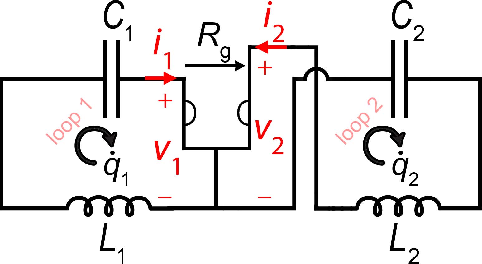
Figure 4. The two-loop nonreciprocal circuit coupled by an ideal gyrator. For specific combinations of values $L_{1}$, $C_{1}$, $L_{2}$, and $C_{2}$, the evolution matrix of the nonreciprocal circuit develops a degeneracy, and its nontrivial Jordan canonical form consists of exactly two Jordan blocks of size 2. A change in the sign of $R_{\mathrm{g}}$ is equivalent to reversing the gyration resistance direction (indicated by the arrow below $R_{\mathrm{g}}$) in this circuit.

$$v_{1}=-R_{\mathrm{g}}i_{2}=-R_{\mathrm{g}}\dot{q}_{2},$$ (7.1a)

$$v_{2}=R_{\mathrm{g}}i_{1}=R_{\mathrm{g}}\dot{q}_{1}.$$ (7.1b)

where $q_{j}$ ($j=1,2$) are the charges associated with currents of gyrator. The coefficient $R_{\mathrm{g}}$ is called gyration resistance and the corresponding antisymmetric impedance matrix of the gyrator is given by

$$Z_{\mathrm{g}}=\left[\begin{array}[]{rr}0&R_{\mathrm{g}}\\ -R_{\mathrm{g}}&0\end{array}\right]=\left(-Z_{\mathrm{g}}\right)^{\mathrm{T}}.$$ (7.2)

The Lagrangian associated with the gyrator element is given by

$$\mathcal{L}_{\mathrm{g}}=\frac{R_{\mathrm{g}}\left(q_{1}\partial_{t}q_{2}-q_{2}\partial_{t}q_{1}\right)}{2}.$$ (7.3)

The simple form of the GNC to obtain second-order degeneracy is shown in Figure 4 and analyzed in the following. The circuit is composed of two LC loops coupled by a gyrator, and we study this circuit without imposing any assumptions on the circuit parameters $L_{1}$, $C_{1}$, $L_{2}$, $C_{2}$ and $R_{\mathrm{g}}$ except that they are all real and non-zero. The Lagrangian of the GNC is described as

$$\left.\mathcal{L}_{\mathrm{nr}}\left(\mathrm{q}_{\mathrm{nr}},\partial_{t}\mathrm{q}_{\mathrm{nr}}\right)\right|_{\Theta_{\mathrm{nr}}}=\frac{L_{1}\left(\partial_{t}q_{1}\right)^{2}}{2}+\frac{L_{2}\left(\partial_{t}q_{2}\right)^{2}}{2}-\frac{\left(q_{1}\right)^{2}}{2C_{1}}-\frac{\left(q_{2}\right)^{2}}{2C_{2}}+\frac{R_{\mathrm{g}}\left(q_{1}\partial_{t}q_{2}-q_{2}\partial_{t}q_{1}\right)}{2},$$ (7.4a)

$$q_{j}\left(t\right)=\int^{t}i_{j}\left(t^{\prime}\right)\,\mathrm{d}t^{\prime},\quad j=1,2,$$ (7.4b)

where the last term in Equation (7.4a) is the source of nonreciprocity in the circuit and we will discuss it later in Subsection 8.1. Also, $q_{j}$ and $i_{j}$ are the charges and the currents associated with loops of the GNC depicted in Figure 4, $\Theta_{\mathrm{nr}}=\left\{L_{1},L_{2},C_{1},C_{2},R_{\mathrm{g}}\right\}$ is the set of circuit’s parameters and we define the vector of charges for the GNC as $\mathrm{q}_{\mathrm{nr}}=\left[q_{1},q_{2}\right]^{\mathrm{T}}$. In nonreciprocal systems, due to the breaking of time reversal symmetry, the Lagrangian associated with the GNC leads to $\mathcal{L}_{\mathrm{nr}}\left(\mathrm{q}_{\mathrm{nr}},\partial_{t}\mathrm{q}_{\mathrm{nr}}\right)\neq\mathcal{L}_{\mathrm{nr}}\left(\mathrm{q}_{\mathrm{nr}},-\partial_{t}\mathrm{q}_{\mathrm{nr}}\right)$. The corresponding evolution equations after simplification, i.e., the Euler-Lagrange equations, are expressed as

$$L_{1}\ddot{q}_{1}-R_{\mathrm{g}}\dot{q_{2}}+\frac{1}{C_{1}}q_{1}=0,$$ (7.5a)

$$L_{2}\ddot{q}_{2}+R_{\mathrm{g}}\dot{q_{1}}+\frac{1}{C_{2}}q_{2}=0.$$ (7.5b)

The second-order differential equations in Equations (7.5a) and (7.5b) are reduced to the standard first-order vector differential equation as

$$\partial_{t}\mathsf{q}_{\mathrm{nr}}=\mathscr{C}_{\mathrm{nr}}\mathsf{q}_{\mathrm{nr}},\quad\mathscr{C}_{\mathrm{nr}}=\left[\begin{array}[]{rrrr}0&0&1&0\\ 0&0&0&1\\ -\frac{1}{L_{1}C_{1}}&0&0&\frac{R_{g}}{L_{1}}\\ 0&-\frac{1}{L_{2}C_{2}}&-\frac{R_{g}}{L_{2}}&0\end{array}\right],$$ (7.6)

where the circuit state vector is defined as $\mathsf{q}_{\mathrm{nr}}=\left[\mathrm{q}_{\mathrm{nr}},\partial_{t}\mathrm{q}_{\mathrm{nr}}\right]^{\mathrm{T}}$and $\mathscr{C}_{\mathrm{nr}}$ is the $4\times 4$ circuit matrix for the GNC. A matrix representation of evolution equations is easily achieved by recasting them as follows:

$$\mathrm{A}_{\mathrm{nr}}\left(s\right)\mathrm{q}_{\mathrm{nr}}=0,\quad\mathrm{A}_{\mathrm{nr}}\left(s\right)=\left[\begin{array}[]{rr}s^{2}+\frac{1}{L_{1}C_{1}}&-s\frac{R_{\mathrm{g}}}{L_{1}}\\ s\frac{R_{\mathrm{g}}}{L_{2}}&s^{2}+\frac{1}{L_{2}C_{2}}\end{array}\right],\quad\mathrm{q}_{\mathrm{nr}}=\left[\begin{array}[]{c}q_{1}\\ q_{2}\end{array}\right],$$ (7.7)

where $\mathrm{A}_{\mathrm{nr}}\left(s\right)$ is a $2\times 2$ monic matrix polynomial of $s$ of the degree 2 and it is rewritten as

$$\mathrm{A}_{\mathrm{nr}}\left(s\right)=\sum_{j=0}^{2}s^{j}\mathrm{A}_{\mathrm{nr},j}=s^{2}\mathrm{A}_{\mathrm{nr},2}+s\mathrm{A}_{\mathrm{nr},1}+\mathrm{A}_{\mathrm{nr},0},$$ (7.8a)

$$\mathrm{A}_{\mathrm{nr},2}=\left[\begin{array}[]{rr}1&0\\ 0&1\end{array}\right],\quad\mathrm{A}_{\mathrm{nr},1}=\left[\begin{array}[]{rr}0&-\frac{R_{\mathrm{g}}}{L_{1}}\\ \frac{R_{\mathrm{g}}}{L_{2}}&0\end{array}\right],\quad\mathrm{A}_{\mathrm{nr},0}=\left[\begin{array}[]{rr}\frac{1}{L_{1}C_{1}}&0\\ 0&\frac{1}{L_{2}C_{2}}\end{array}\right].$$ (7.8b)

The eigenvalue problem corresponding to the Equation (7.6) is

$$\left(s\mathbb{I}_{4}-\mathscr{C}_{\mathrm{nr}}\right)\mathsf{q}_{\mathrm{nr,s}}=0,\quad\mathsf{q}_{\mathrm{nr,s}}=\left[\begin{array}[]{r}\mathrm{q}_{\mathrm{nr}}\\ s\mathrm{q}_{\mathrm{nr}}\end{array}\right].$$ (7.9)

The associated characteristic polynomial for the GNC is expressed as

$$\chi_{\mathrm{nr}}\left(s\right)=\det\left\{A_{\mathrm{nr}}\left(s\right)\right\}=\det\left\{s\mathbb{I}_{4}-\mathscr{C}_{\mathrm{nr}}\right\}=s^{4}+s^{2}\left(\frac{1}{L_{1}C_{1}}+\frac{1}{L_{2}C_{2}}+\frac{R_{\mathrm{g}}^{2}}{L_{1}L_{2}}\right)+\frac{1}{L_{1}C_{1}L_{2}C_{2}},$$ (7.10)

and the eigenvalues of the eigenvalue problem can be calculated from the characteristic polynomial $\chi_{\mathrm{nr}}\left(s\right)=0$. The further analytical developments suggest to introduce the following variables for the circuit

$$\xi_{1}=\frac{1}{L_{1}C_{1}},\quad\xi_{2}=\frac{1}{L_{2}C_{2}}.$$ (7.11)

In Equation (7.11), $\sqrt{\xi_{1}}$ is the resonance frequency of the first loop and $\sqrt{\xi_{2}}$ is the resonance frequency of the second loop. Alternatively, the companion matrix $\mathscr{C}_{\mathrm{nr}}$ given by Equation (7.6) and its characteristic polynomial as in Equation (7.10) take the following forms

$$\mathscr{C}_{\mathrm{nr}}=\left[\begin{array}[]{rrrr}0&0&1&0\\ 0&0&0&1\\ -\xi_{1}&0&0&\frac{R_{\mathrm{g}}}{L_{1}}\\ 0&-\xi_{2}&-\frac{R_{\mathrm{g}}}{L_{2}}&0\end{array}\right],$$ (7.12a)

$$\chi_{\mathrm{nr}}\left(h\right)=h^{2}+h\left(\xi_{1}+\xi_{2}+\frac{R_{\mathrm{g}}^{2}}{L_{1}L_{2}}\right)+\xi_{1}\xi_{2},\quad h=s^{2}.$$ (7.12b)

Considering the degenerate eigenvalues satisfying equation $\chi_{\mathrm{nr}}\left(h\right)=0$, we turn our attention to the discriminant of the quadratic polynomial of Equation (7.12b),

$$\Delta_{\mathrm{nr},h}=\frac{R_{\mathrm{g}}^{4}}{L_{1}^{2}L_{2}^{2}}+\frac{2\left(\xi_{1}+\xi_{2}\right)R_{\mathrm{g}}^{2}}{L_{1}L_{2}}+\left(\xi_{1}-\xi_{2}\right)^{2},$$ (7.13)

where the solutions of the quadratic equation of Equation (7.12b) are

$$h_{\pm}=\frac{-\left(\xi_{1}+\xi_{2}+\frac{R_{g}^{2}}{L_{1}L_{2}}\right)\pm\sqrt{\Delta_{\mathrm{nr},h}}}{2}.$$ (7.14)

The corresponding four solutions $s$ of the characteristic polynomial are given by

$$s=\pm\sqrt{h_{+}},\pm\sqrt{h_{-}},$$ (7.15)

In this case, the eigenvalue degeneracy condition becomes $\Delta_{\mathrm{nr},h}=0$. It is possible to view degeneracy condition equation as a constraint on the coefficients of the quadratic in polynomial $\chi_{\mathrm{nr}}\left(h\right)=0$ and consequently on the circuit parameters, namely

$$L_{1}^{2}L_{2}^{2}\Delta_{\mathrm{nr},h}=g^{2}+2\left(\xi_{1}+\xi_{2}\right)gL_{1}L_{2}+\left(\xi_{1}-\xi_{2}\right)^{2}L_{1}^{2}L_{2}^{2}=0,\quad g=R_{\mathrm{g}}^{2},$$ (7.16)

and we refer to positive $g$ as the gyration resistance square. Since $R_{\mathrm{g}}$ is real, then $g=R_{\mathrm{g}}^{2}$ is real as well. Equation (7.16) is a quadratic equation for $g$, which has exactly two solutions of

$$g_{\mathrm{d,\pm}}=-L_{1}L_{2}\left(\sqrt{\xi_{1}}\mp\sqrt{\xi_{2}}\right)^{2},$$ (7.17)

which lead to two degenerate cases. For the two special value of gyration resistance square $g_{\mathrm{d,\pm}}$, we get two degenerate roots for $h_{\pm}$ as

$$h_{\mathrm{d,}\pm}=-\frac{\xi_{1}+\xi_{2}+\frac{g_{\mathrm{d,\pm}}}{L_{1}L_{2}}}{2}=\mp\sqrt{\xi_{1}\xi_{2}}.$$ (7.18)

Expression of $g_{\mathrm{d,\pm}}$ shown in Equation (7.17) is real-valued if and only if $\xi_{1}\xi_{2}>0$, or equivalently $\xi_{1}/\left|\xi_{1}\right|=\xi_{2}/\left|\xi_{2}\right|=\pm 1$. Also, the Jordan canonical form out of degeneracy condition, i.e., $\Delta_{\mathrm{nr},h}\neq 0$, is expressed as

$$\mathscr{J}_{\mathrm{r}}=\left[\begin{array}[]{rrrr}\mathrm{i}s_{1}&0&0&0\\ 0&-\mathrm{i}s_{1}&0&0\\ 0&0&\mathrm{i}s_{2}&0\\ 0&0&0&-\mathrm{i}s_{2}\end{array}\right],\quad\begin{array}[]{c}s_{1}=\sqrt{\frac{\xi_{\mathrm{s}}+\sqrt{L_{1}^{2}L_{2}^{2}\Delta_{\mathrm{nr},h}}}{2L_{1}L_{2}}}\\ s_{2}=\sqrt{\frac{\xi_{\mathrm{s}}-\sqrt{L_{1}^{2}L_{2}^{2}\Delta_{\mathrm{nr},h}}}{2L_{1}L_{2}}}\end{array},\quad\xi_{\mathrm{s}}=\left(\xi_{1}+\xi_{2}\right)L_{1}L_{2}+R_{\mathrm{g}}^{2},$$ (7.19)

where $\pm\mathrm{i}s_{i}$ ($i=1,2$) are the non-degenerate eigenvalues of the corresponding companion matrix. We write down eigenvectors corresponding to the calculated non-degenerate eigenvalues as (when $\Delta_{\mathrm{nr},h}\neq 0$)

$$\mathscr{V}_{\mathrm{nr}}=\left[\mathsf{e}_{\mathrm{nr},+s_{1}}|\mathsf{e}_{\mathrm{nr},-s_{1}}|\mathsf{e}_{\mathrm{nr},+s_{2}}|\mathsf{e}_{\mathrm{nr},-s_{2}}\right],$$ (7.20a)

$$\begin{array}[]{c}\mathsf{e}_{\mathrm{nr},\pm s_{i}}=\left[\begin{array}[]{r}\frac{2R_{\mathrm{g}}^{2}+2L_{1}L_{2}\xi_{2}-\xi_{\mathrm{s}}-\sqrt{L_{1}^{2}L_{2}^{2}\Delta_{\mathrm{nr},h}}}{2L_{1}R_{\mathrm{g}}\xi_{1}}\\ \mp\frac{L_{1}L_{2}\left(-s_{i}^{2}\right)^{3/2}+\xi_{\mathrm{s}}\sqrt{-s_{i}^{2}}}{L_{1}L_{2}\xi_{1}\xi_{2}}\\ \pm\frac{L_{1}L_{2}\left(-s_{i}^{2}\right)^{3/2}+\left(R_{\mathrm{g}}^{2}+L_{1}L_{2}\xi_{2}\right)\sqrt{-s_{i}^{2}}}{L_{1}R_{\mathrm{g}}\xi_{1}}\\ 1\end{array}\right].\end{array}$$ (7.20b)

There were two values for the degenerate gyration resistance square as shown in Equation (7.17), resulting in degenerate purely imaginary or purely real eigenvalues. Firstly, if we consider $g=g_{\mathrm{d},+}=-L_{1}L_{2}\left(\sqrt{\xi_{1}}-\sqrt{\xi_{2}}\right)^{2}$, the degenerate characteristic polynomial is given by

$$\chi_{\mathrm{nr,+}}\left(s\right)=s^{4}+2s^{2}\sqrt{\xi_{1}\xi_{2}}+\xi_{1}\xi_{2}=\left(s^{2}+\sqrt{\xi_{1}\xi_{2}}\right)^{2}=0.$$ (7.21)

Then, the corresponding degenerate companion matrix $\mathscr{C}_{\mathrm{nr,+}}$ by substituting $g=g_{\mathrm{d},+}$ is rewritten as

$$\mathscr{C}_{\mathrm{nr,+}}=\left[\begin{array}[]{rrrr}0&0&1&0\\ 0&0&0&1\\ -\xi_{1}&0&0&\sqrt{\frac{g_{\mathrm{d},+}}{L_{1}^{2}}}\\ 0&-\xi_{2}&-\sqrt{\frac{g_{\mathrm{d},+}}{L_{2}^{2}}}&0\end{array}\right].$$ (7.22)

.

The Jordan canonical form of the companion matrix $\mathscr{C}_{\mathrm{nr,+}}$ with purely imaginary eigenvalues (purely real eigenfrequencies) is described by

$$\mathscr{J}_{\mathrm{nr,+}}=\left[\begin{array}[]{rrrr}\mathrm{i}s_{\mathrm{e}}&1&0&0\\ 0&\mathrm{i}s_{\mathrm{e}}&0&0\\ 0&0&-\mathrm{i}s_{\mathrm{e}}&1\\ 0&0&0&-\mathrm{i}s_{\mathrm{e}}\end{array}\right],\quad s_{\mathrm{e}}=\left(\xi_{\mathrm{e}}\right)^{\frac{1}{2}}=\left(\xi_{1}\xi_{2}\right)^{\frac{1}{4}}.$$ (7.23)

Accordingly, the Jordan basis of the companion matrix $\mathscr{C}_{\mathrm{nr,+}}$ is calculated as

$$\mathscr{Z}_{\mathrm{nr,+}}=\left[\begin{array}[]{rrrr}\frac{\sqrt{\xi_{1}\xi_{2}}-\xi_{1}}{4\mathrm{i}\sqrt{\xi_{\mathrm{e}}}}&\frac{1}{2}&-\frac{\sqrt{\xi_{1}\xi_{2}}-\xi_{1}}{4\mathrm{i}\sqrt{\xi_{\mathrm{e}}}}&\frac{1}{2}\\ -\frac{\xi_{1}\sqrt{L_{1}L_{2}\left(2\xi_{\mathrm{e}}-\xi_{1}-\xi_{2}\right)}}{4L_{2}\xi_{\mathrm{e}}}&-\mathrm{i}\frac{\xi_{1}\sqrt{L_{1}L_{2}\left(2\xi_{\mathrm{e}}-\xi_{1}-\xi_{2}\right)}}{4L_{2}\xi_{\mathrm{e}}\sqrt{\xi_{\mathrm{e}}}}&-\frac{\xi_{1}\sqrt{L_{1}L_{2}\left(2\xi_{\mathrm{e}}-\xi_{1}-\xi_{2}\right)}}{4L_{2}\xi_{\mathrm{e}}}&\mathrm{i}\frac{\xi_{1}\sqrt{L_{1}L_{2}\left(2\xi_{\mathrm{e}}-\xi_{1}-\xi_{2}\right)}}{4L_{2}\xi_{\mathrm{e}}\sqrt{\xi_{\mathrm{e}}}}\\ \frac{\xi_{1}\left(\xi_{2}-\xi_{\mathrm{e}}\right)}{4\xi_{\mathrm{e}}}&-\frac{\xi_{1}\left(\xi_{2}+\xi_{\mathrm{e}}\right)}{4\mathrm{i}\xi_{\mathrm{e}}\sqrt{\xi_{\mathrm{e}}}}&\frac{\xi_{1}\left(\xi_{2}-\xi_{\mathrm{e}}\right)}{4\xi_{\mathrm{e}}}&\frac{\xi_{1}\left(\xi_{2}+\xi_{\mathrm{e}}\right)}{4\mathrm{i}\xi_{\mathrm{e}}\sqrt{\xi_{\mathrm{e}}}}\\ \frac{\xi_{1}\sqrt{L_{1}L_{2}\left(2\xi_{\mathrm{e}}-\xi_{1}-\xi_{2}\right)}}{4\mathrm{i}L_{2}\sqrt{\xi_{\mathrm{e}}}}&0&-\frac{\xi_{1}\sqrt{L_{1}L_{2}\left(2\xi_{\mathrm{e}}-\xi_{1}-\xi_{2}\right)}}{4\mathrm{i}L_{2}\sqrt{\xi_{\mathrm{e}}}}&0\end{array}\right].$$ (7.24)

Secondly, if we consider $g=g_{\mathrm{d},-}=-L_{1}L_{2}\left(\xi_{1}+\xi_{2}+2\sqrt{\xi_{1}\xi_{2}}\right)$, the degenerate characteristic polynomial is rewritten as

$$\chi_{\mathrm{nr,-}}\left(s\right)=s^{4}-2s^{2}\sqrt{\xi_{1}\xi_{2}}+\xi_{1}\xi_{2}=\left(s^{2}-\sqrt{\xi_{1}\xi_{2}}\right)^{2}=0.$$ (7.25)

Then, the degenerate corresponding companion matrix $\mathscr{C}_{\mathrm{nr,-}}$ is rewritten as

$$\mathscr{C}_{\mathrm{nr,-}}=\left[\begin{array}[]{rrrr}0&0&1&0\\ 0&0&0&1\\ -\xi_{1}&0&0&-\sqrt{\frac{g_{\mathrm{d},-}}{L_{1}^{2}}}\\ 0&-\xi_{2}&\sqrt{\frac{g_{\mathrm{d},-}}{L_{2}^{2}}}&0\end{array}\right].$$ (7.26)

The Jordan canonical form of the companion matrix $\mathscr{C}_{\mathrm{nr,-}}$ with purely real eigenvalues (purely imaginary eigenfrequencies) is expressed by

$$\mathscr{J}_{\mathrm{nr,-}}=\left[\begin{array}[]{rrrr}s_{\mathrm{e}}&1&0&0\\ 0&s_{\mathrm{e}}&0&0\\ 0&0&-s_{\mathrm{e}}&1\\ 0&0&0&-s_{\mathrm{e}}\end{array}\right].$$ (7.27)

Finally, the Jordan basis of the companion matrix $\mathscr{C}_{\mathrm{nr,-}}$ is obtained as

$$\mathscr{Z}_{\mathrm{nr,-}}=\left[\begin{array}[]{rrrc}-\frac{\sqrt{\xi_{1}\xi_{2}}+\xi_{1}}{4\sqrt{\xi_{\mathrm{e}}}}&\frac{1}{2}&\frac{\sqrt{\xi_{1}\xi_{2}}+\xi_{1}}{4\sqrt{\xi_{\mathrm{e}}}}&\frac{1}{2}\\ \mathrm{i}\frac{\xi_{1}\sqrt{L_{1}L_{2}\left(2\xi_{\mathrm{e}}+\xi_{1}+\xi_{2}\right)}}{4L_{2}\xi_{\mathrm{e}}}&-\mathrm{i}\frac{\xi_{1}\sqrt{L_{1}L_{2}\left(2\xi_{\mathrm{e}}+\xi_{1}+\xi_{2}\right)}}{4L_{2}\xi_{\mathrm{e}}\sqrt{\xi_{\mathrm{e}}}}&\mathrm{i}\frac{\xi_{1}\sqrt{L_{1}L_{2}\left(2\xi_{\mathrm{e}}+\xi_{1}+\xi_{2}\right)}}{4L_{2}\xi_{\mathrm{e}}}&\mathrm{i}\frac{\xi_{1}\sqrt{L_{1}L_{2}\left(2\xi_{\mathrm{e}}+\xi_{1}+\xi_{2}\right)}}{4L_{2}\xi_{\mathrm{e}}\sqrt{\xi_{\mathrm{e}}}}\\ -\frac{\xi_{1}\left(\xi_{2}+\xi_{\mathrm{e}}\right)}{4\xi_{\mathrm{e}}}&\frac{\xi_{1}\left(\xi_{2}-\xi_{\mathrm{e}}\right)}{4\xi_{\mathrm{e}}\sqrt{\xi_{\mathrm{e}}}}&-\frac{\xi_{1}\left(\xi_{2}+\xi_{\mathrm{e}}\right)}{4\xi_{\mathrm{e}}}&-\frac{\xi_{1}\left(\xi_{2}-\xi_{\mathrm{e}}\right)}{4\xi_{\mathrm{e}}\sqrt{\xi_{\mathrm{e}}}}\\ \mathrm{i}\frac{\xi_{1}\sqrt{L_{1}L_{2}\left(2\xi_{\mathrm{e}}+\xi_{1}+\xi_{2}\right)}}{4L_{2}\sqrt{\xi_{\mathrm{e}}}}&0&-\mathrm{i}\frac{\xi_{1}\sqrt{L_{1}L_{2}\left(2\xi_{\mathrm{e}}+\xi_{1}+\xi_{2}\right)}}{4L_{2}\sqrt{\xi_{\mathrm{e}}}}&0\end{array}\right].$$ (7.28)

The fundamental of Lagrangian for a linear system is explained in Subsection 6.1 and the associated coefficients for the GNC are given by

$$\alpha_{\mathrm{nr}}=\left[\begin{array}[]{rr}L_{1}&0\\ 0&L_{2}\end{array}\right],\quad\theta_{\mathrm{nr}}=\left[\begin{array}[]{rr}0&-\frac{R_{\mathrm{g}}}{2}\\ \frac{R_{\mathrm{g}}}{2}&0\end{array}\right],\quad\eta_{\mathrm{nr}}=\left[\begin{array}[]{rr}\frac{1}{C_{1}}&0\\ 0&\frac{1}{C_{2}}\end{array}\right].$$ (7.29)

It follows from Equation (6.10) that the necessary and sufficient condition of the nonreciprocity is $\theta_{\mathrm{nr}}\neq\theta_{\mathrm{nr}}^{\mathrm{T}}$. Then, the Lagrangian equation of GNC is written as follows:

$$\mathcal{L}_{\mathrm{nr}}\left(\mathrm{q}_{\mathrm{nr}},\partial_{t}\mathrm{q}_{\mathrm{nr}}\right)=\frac{1}{2}\left[\begin{array}[]{r}\mathrm{q}_{\mathrm{nr}}\\ \partial_{t}\mathrm{q}_{\mathrm{nr}}\end{array}\right]^{\mathrm{T}}\mathrm{M}_{\mathrm{L,nr}}\left[\begin{array}[]{r}\mathrm{q}_{\mathrm{nr}}\\ \partial_{t}\mathrm{q}_{\mathrm{nr}}\end{array}\right],$$ (7.30a)

$$\mathrm{M}_{\mathrm{L,nr}}=\left[\begin{array}[]{rrrr}-\frac{1}{C_{1}}&0&0&\frac{\mathit{R_{\mathrm{g}}}}{2}\\ 0&-\frac{1}{C_{2}}&-\frac{\mathit{R_{\mathrm{g}}}}{2}&0\\ 0&-\frac{\mathit{R_{\mathrm{g}}}}{2}&L_{1}&0\\ \frac{\mathit{R_{\mathrm{g}}}}{2}&0&0&L_{2}\end{array}\right].$$ (7.30b)

Moreover, the Hamiltonian formulation can also be used to show the GNC characteristics (see Subsection 6.2 for more information). Then, the $4\times 4$ matrix $\mathrm{M}_{\mathrm{H,nr}}$ required for the Hamiltonian formulation is given by

$$\mathrm{M}_{\mathrm{H,nr}}=\left[\begin{array}[]{rrrr}\frac{R_{\mathrm{g}}^{2}}{4L_{2}}+\frac{1}{C_{1}}&0&0&-\frac{R_{\mathrm{g}}}{2L_{2}}\\ 0&\frac{R_{\mathrm{g}}^{2}}{4L_{1}}+\frac{1}{C_{2}}&\frac{R_{\mathrm{g}}}{2L_{1}}&0\\ 0&\frac{\mathit{R_{\mathrm{g}}}}{2L_{1}}&\frac{1}{L_{1}}&0\\ -\frac{R_{\mathrm{g}}}{2L_{2}}&0&0&\frac{1}{L_{2}}\end{array}\right].$$ (7.35)

Ultimately, the Hamiltonian matrix for the GNC is given by by

$$\mathscr{H}_{\mathrm{nr}}=\mathbb{J}\mathrm{M}_{\mathrm{H,nr}}=\left[\begin{array}[]{rrrr}0&\frac{\mathit{R_{\mathrm{g}}}}{2L_{1}}&\frac{1}{L_{1}}&0\\ -\frac{\mathit{R_{\mathrm{g}}}}{2L_{2}}&0&0&\frac{1}{L_{2}}\\ -\frac{\mathit{R_{\mathrm{g}}^{2}}}{4L_{2}}-\frac{1}{C_{1}}&0&0&\frac{\mathit{R_{\mathrm{g}}}}{2L_{2}}\\ 0&-\frac{\mathit{R_{\mathrm{g}}^{2}}}{4L_{1}}-\frac{1}{C_{2}}&-\frac{\mathit{R_{\mathrm{g}}}}{2L_{1}}&0\end{array}\right].$$ (7.36)

According to Equation (6.15), we can see that in the nonreciprocal circuit with $\theta_{\mathrm{nr}}\neq 0$, the relation between the momentum $\mathrm{p}_{\mathrm{nr}}$ and the current $\partial_{t}\mathrm{q}_{\mathrm{nr}}$ also depends on the charge $\mathrm{q}_{\mathrm{nr}}$. In addition, it is important to point out that a circuit with gyrators does not necessarily guarantee nonreciprocity, but it can lead to nonreciprocity.

8. Analysis of Reciprocity and Nonreciprocity

In this section, we analyze reciprocity properties in both reciprocal and nonreciprocal circuits. This particular feature will be explored in the Lagrangian and eigenvectors of both PRC and GNC.

8.1. Lagrangian

According to investigation provided in Section 4, the Lagrangian associated with the PRC is depicted as

$$\left.\mathcal{L}_{\mathrm{r}}\left(\mathrm{q}_{\mathrm{r}},\partial_{t}\mathrm{q}_{\mathrm{r}}\right)\right|_{\Theta_{\mathrm{r}}}=\frac{L_{1}\left(\partial_{t}q_{1}\right)^{2}}{2}+\frac{L_{0}\left(\partial_{t}q_{0}\right)^{2}}{2}-\frac{\left(q_{1}\right)^{2}}{2C_{1}}-\frac{\left(q_{1}-q_{0}\right)^{2}}{2C_{0}}.$$ (8.1)

An arrow of time is a concept that proposes the "one-way direction" or "asymmetry" of time. If we change the direction of arrow of time, the Lagrangian associated with PRC is expressed by

$$\left.\mathcal{L}_{\mathrm{r}}\left(\mathrm{q}_{\mathrm{r}},-\partial_{t}\mathrm{q}_{\mathrm{r}}\right)\right|_{\Theta_{\mathrm{r}}}=\frac{L_{1}\left(\partial_{t}q_{1}\right)^{2}}{2}+\frac{L_{0}\left(\partial_{t}q_{0}\right)^{2}}{2}-\frac{\left(q_{1}\right)^{2}}{2C_{1}}-\frac{\left(q_{1}-q_{0}\right)^{2}}{2C_{0}}.$$ (8.2)

By comparing Equations (8.1) and (8.2) we have

$$\left.\mathcal{L}_{\mathrm{r}}\left(\mathrm{q}_{\mathrm{r}},\partial_{t}\mathrm{q}_{\mathrm{r}}\right)\right|_{\Theta_{\mathrm{r}}}=\left.\mathcal{L}_{\mathrm{r}}\left(\mathrm{q}_{\mathrm{r}},-\partial_{t}\mathrm{q}_{\mathrm{r}}\right)\right|_{\Theta_{\mathrm{r}}}.$$ (8.3)

In the above equation, we can see that there is symmetry in time, which refers to reciprocity within the PRC (see Definition 2).

Definition 2 (Lagrangian of reciprocal and nonreciprocal systems).

For a system described by coordinates $F=\left.\left[f_{i}\right]\right|_{i=1}^{n}$ and time $t$, the time reversal symmetry can be formulated as follows. For any trajectory $F\left(t\right)$ of the system, $\tilde{F}\left(t\right)=F\left(-t\right)$ is also its trajectory. In terms of the Lagrangian function $\mathcal{L}=\mathcal{L}\left(F,\dot{F}\right)$, it means the invariance of Lagrangian function under the transformation $\dot{F}\rightarrow-\dot{F}$ [33]:

$$\mathcal{L}\left(F,\dot{F}\right)=\mathcal{L}\left(F,-\dot{F}\right).$$ (8.4)

Also, for a system with broken time reversal symmetry we observe $\mathcal{L}\left(F,\dot{F}\right)\neq\mathcal{L}\left(F,-\dot{F}\right)$.

On the other hand, based on the expression given in Section 7, the Lagrangian associated with GNC is expressed by

$$\left.\mathcal{L}_{\mathrm{nr}}\left(\mathrm{q}_{\mathrm{nr}},\partial_{t}\mathrm{q}_{\mathrm{nr}}\right)\right|_{\Theta_{\mathrm{nr}}}=\frac{L_{1}\left(\partial_{t}q_{1}\right)^{2}}{2}+\frac{L_{2}\left(\partial_{t}q_{2}\right)^{2}}{2}-\frac{\left(q_{1}\right)^{2}}{2C_{1}}-\frac{\left(q_{2}\right)^{2}}{2C_{2}}+\frac{R_{\mathrm{g}}\left(q_{1}\partial_{t}q_{2}-q_{2}\partial_{t}q_{1}\right)}{2}.$$ (8.5)

Then, by inverting the direction of the time we have

$$\left.\mathcal{L}_{\mathrm{nr}}\left(\mathrm{q}_{\mathrm{nr}},-\partial_{t}\mathrm{q}_{\mathrm{nr}}\right)\right|_{\Theta_{\mathrm{nr}}}=\frac{L_{1}\left(\partial_{t}q_{1}\right)^{2}}{2}+\frac{L_{2}\left(\partial_{t}q_{2}\right)^{2}}{2}-\frac{\left(q_{1}\right)^{2}}{2C_{1}}-\frac{\left(q_{2}\right)^{2}}{2C_{2}}-\frac{R_{\mathrm{g}}\left(q_{1}\partial_{t}q_{2}-q_{2}\partial_{t}q_{1}\right)}{2},$$ (8.6)

where we observe the sign of nonreciprocity in the last term of the above equation. Now, by inverting the direction of gyration resistance ($R_{\mathrm{g}}\rightarrow-R_{\mathrm{g}}$) in addition to reversing the direction of time, we rewrite the Lagrangian associated with the new circuit by using a new set of parameters $\widetilde{\Theta}_{\mathrm{nr}}=\left\{L_{1},L_{2},C_{1},C_{2},-R_{\mathrm{g}}\right\}$ as

$$\left.\mathcal{L}_{\mathrm{nr}}\left(\mathrm{q}_{\mathrm{nr}},-\partial_{t}\mathrm{q}_{\mathrm{nr}}\right)\right|_{\widetilde{\Theta}_{\mathrm{nr}}}=\frac{L_{1}\left(\partial_{t}q_{1}\right)^{2}}{2}+\frac{L_{2}\left(\partial_{t}q_{2}\right)^{2}}{2}-\frac{\left(q_{1}\right)^{2}}{2C_{1}}-\frac{\left(q_{2}\right)^{2}}{2C_{2}}+\frac{R_{\mathrm{g}}\left(q_{1}\partial_{t}q_{2}-q_{2}\partial_{t}q_{1}\right)}{2}.$$ (8.7)

Finally, by comparing Equations (8.5), (8.6) and (8.7), we have

$$\left.\mathcal{L}_{\mathrm{nr}}\left(\mathrm{q}_{\mathrm{nr}},\partial_{t}\mathrm{q}_{\mathrm{nr}}\right)\right|_{\Theta_{\mathrm{nr}}}=\left.\mathcal{L}_{\mathrm{nr}}\left(\mathrm{q}_{\mathrm{nr}},-\partial_{t}\mathrm{q}_{\mathrm{nr}}\right)\right|_{\widetilde{\Theta}_{\mathrm{nr}}}\neq\left.\mathcal{L}_{\mathrm{nr}}\left(\mathrm{q}_{\mathrm{nr}},-\partial_{t}\mathrm{q}_{\mathrm{nr}}\right)\right|_{\Theta_{\mathrm{nr}}},$$ (8.8)

which demonstrate the nonreciprocity in the GNC (see Definition 2). In spite of this, the circuit with the same Lagrangian is achieved by simultaneously inverting the direction of the time and gyration resistance. Alternately, by removing the source of nonreciprocity in the circuit, i.e., the gyrator, the circuit becomes a reciprocal circuit composed of two uncoupled LC resonators. The properties of a single LC resonator are discussed in Appendix C.

8.2. Eigenvectors

As explained in Subsection 5.2, the eigenvectors associated to the PRC in the general form are expressed as

$$\begin{array}[]{c}\mathsf{e}_{\mathrm{r,}\pm s_{i}}=\left[\begin{array}[]{c}\mathsf{q}_{\pm s_{i}}\\ \dot{\mathsf{q}}_{\pm s_{i}}\end{array}\right]\stackrel{{\scriptstyle\mathrm{def}}}{{=}}\left[\begin{array}[]{r}\mp\frac{\left(-s_{i}^{2}\right)^{3/2}+\left(\xi_{0}+\delta\right)\sqrt{-s_{i}^{2}}}{\xi_{0}\xi_{1}}\\ \mp\frac{\left(-s_{i}^{2}\right)^{3/2}+\xi_{\mathrm{s}}\sqrt{-s_{i}^{2}}}{\xi_{0}\xi_{i}}\\ 1-\frac{s_{i}^{2}}{\xi_{0}}\\ 1\end{array}\right],\quad\xi_{\mathrm{s}}=\xi_{1}+\xi_{0}+\delta,\end{array}\quad i=1,2.$$ (8.9)

Due to reciprocity, we observe the change in the sign of charges when we inverse the sign of $s_{i}$ ($i=1,2$), i.e., $\mathsf{q}_{+s_{i}}=-\mathsf{q}_{-s_{i}}$ ($i=1,2$), whereas the sign of the first derivative of charges remains constant, i.e., $\dot{\mathsf{q}}_{+s_{i}}=\dot{\mathsf{q}}_{-s_{i}}$ ($i=1,2$). The reciprocity feature of PRC is evident from these properties.

Next, we study the GNC eigenvectors to explore a reciprocity feature. Based on the presented expression in Section 7, the eigenvectors associated to the GNC are presented as

$$\begin{array}[]{c}\mathsf{e}_{\mathrm{nr,}\pm s_{i}}=\left[\begin{array}[]{c}\mathsf{q}_{\pm s_{i}}\\ \dot{\mathsf{q}}_{\pm s_{i}}\end{array}\right]\stackrel{{\scriptstyle\mathrm{def}}}{{=}}\left[\begin{array}[]{r}\frac{2R_{\mathrm{g}}^{2}+2L_{1}L_{2}\xi_{2}-\xi_{\mathrm{s}}-\sqrt{L_{1}^{2}L_{2}^{2}\Delta_{\mathrm{nr},h}}}{2L_{1}R_{\mathrm{g}}\xi_{1}}\\ \mp\frac{L_{1}L_{2}\left(-s_{i}^{2}\right)^{3/2}+\xi_{\mathrm{s}}\sqrt{-s_{i}^{2}}}{L_{1}L_{2}\xi_{1}\xi_{2}}\\ \pm\frac{L_{1}L_{2}\left(-s_{i}^{2}\right)^{3/2}+\left(R_{\mathrm{g}}^{2}+L_{1}L_{2}\xi_{2}\right)\sqrt{-s_{i}^{2}}}{L_{1}R_{\mathrm{g}}\xi_{1}}\\ 1\end{array}\right],\quad\xi_{\mathrm{s}}=\left(\xi_{1}+\xi_{2}\right)L_{1}L_{2}+R_{\mathrm{g}}^{2},\quad i=1,2.\end{array}$$ (8.10)

We cannot observe the same behavior for the sign of charges and their first derivative from the above expression for the eigenvectors of the GNC, i.e., $\mathsf{q}_{+s_{i}}\neq-\mathsf{q}_{-s_{i}}$, $\dot{\mathsf{q}}_{+s_{i}}\neq\dot{\mathsf{q}}_{-s_{i}}$($i=1,2$). In light of these eigenvector properties, it can be concluded that GNC is not reciprocal.

Remark 3 (Nonreciprocity and symmetries of the set of eigenvectors).

Our studies indicate that nonreciprocity is manifested in the breakdown of natural symmetries of the set of eigenvectors rather than eigenvalues. Indeed, the Lagrangian and eigenvectors of a circuit are capable of reflecting the reciprocity properties of the circuit. Despite this, nonreciprocity cannot be captured in the Jordan canonical form and consequently in the eigenvalues of the circuit matrix.

We demonstrated that the Jordan canonical form of the circuit does not reflect reciprocity. Consequently, despite the fact that reciprocal and nonreciprocal circuits differ from many perspectives, these two circuits with different topologies can produce the same Jordan canonical form under certain conditions.

9. Reciprocal and Nonreciprocal Circuits Transformation

9.1. Equivalency condition in characteristic polynomial

By comparing the characteristic polynomial of the PRC expressed in Equation (4.5) and the characteristic polynomial of the GNC stated in Equation (7.11) we observe the conditions to obtain equivalency between the characteristic polynomials of these two circuits by equating coefficients as

$$\left\{\begin{array}[]{l}\left\{s^{1}\right\}:\frac{R_{\mathrm{g}}^{2}}{L_{1}L_{2}}+\frac{1}{L_{2}C_{2}}+\frac{1}{L_{1}C_{1}}=\frac{1}{L_{1}C_{0}}+\frac{1}{L_{0}C_{0}}+\frac{1}{L_{1}C_{1}}\\ \left\{s^{0}\right\}:\frac{1}{L_{1}C_{1}L_{2}C_{2}}=\frac{1}{L_{0}C_{0}L_{1}C_{1}}\end{array}\right.$$ (9.1)

Then, we suppose that the first fundamental loop (that include $L_{1}$ and $C_{1}$) in both circuits has the same resonance frequency. So, the conditions to have the same Jordan canonical form for both PRC and GNC are summarized as follows:

$$R_{\mathrm{g}}^{2}=R_{\mathrm{g,eq}}^{2}=\frac{L_{2}}{C_{0}}=\frac{L_{0}}{C_{2}},$$ (9.2)

where $R_{\mathrm{g,eq}}$ is the equivalency value of gyration resistance that can be used to get the same eigenfrequencies in PRC and GNC.

9.2. Equivalent circuit representation

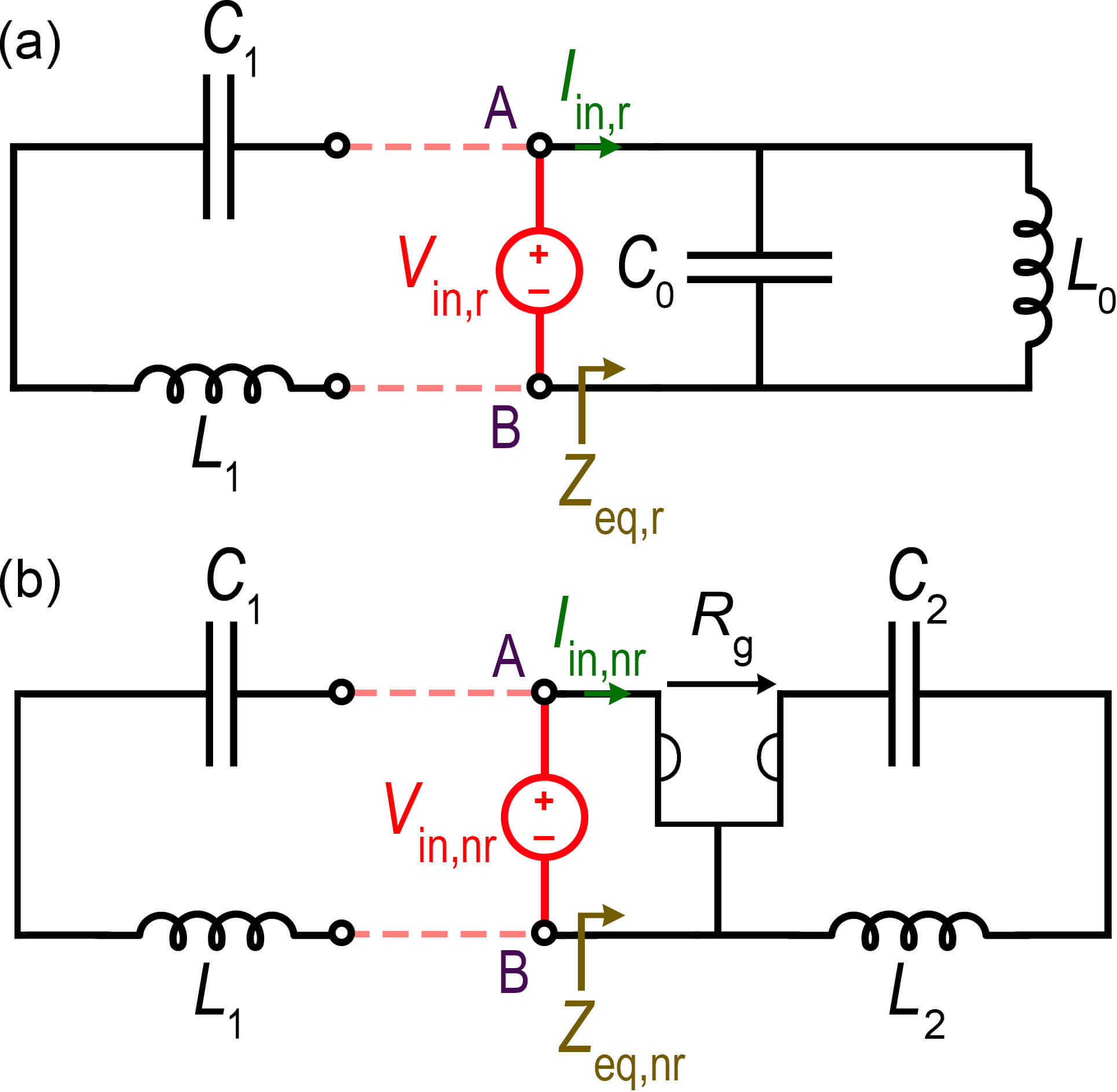
Figure 5. The equivalent circuit and the condition for obtaining (a) reciprocal and (b) nonreciprocal circuits with the same Jordan canonical forms and consequently the same eigenfrequencies by selecting the equivalency value for the gyration resistance $R_{\mathrm{g,eq}}$. The right side of both circuits can have the same equivalent impedance value if $R_{\mathrm{g,eq}}=\sqrt{L_{0}/C_{2}}=\sqrt{L_{2}/C_{0}}$. The left loop in both circuits includes a series resonator with the same resonance frequency.

By using the equivalent circuit representation that can be observed from two selected points of a desired network, we can determine the equivalency condition between reciprocal and nonreciprocal circuits [34, 35]. As originally described in network theory, Thévenin’s theorem asserts that “for any linear electrical network with only voltage and current sources, and impedances can be substituted at input ports by using a combination of an equivalent impedance $Z_{\mathrm{Th}}$ in a series connection with an equivalent voltage source $V_{\mathrm{Th}}$”. The equivalent impedance $Z_{\mathrm{Th}}$ is the impedance observed from the input port if all ideal current sources in the circuit were substituted by an open circuit and all ideal voltage sources were substituted by a short circuit. Also, the equivalent voltage $V_{\mathrm{Th}}$ is the voltage calculated at the input port of the circuit when the input port is open. In the case of a short circuit at the input port, the current flowing from the short circuit would be $I_{\mathrm{Th}}=V_{\mathrm{Th}}/Z_{\mathrm{Th}}$. As a result, equivalent impedance $Z_{\mathrm{Th}}$ could also be calculated as $Z_{\mathrm{Th}}=V_{\mathrm{Th}}/I_{\mathrm{Th}}$. To simplify circuit analysis, Thévenin’s theorem and its dual, Norton’s theorem, are often used. By using Thévenin’s theorem, any circuit’s sources and impedances can be converted to a Thévenin equivalents; in some cases, this may be more convenient than Kirchhoff’s voltage and current laws.

According to Figure 5(a), we cut the PRC circuit into two segments and characterize the right segment using the Thévenin’s equivalent circuit. The input impedance $Z_{\mathrm{eq,r}}$, that is identical to the equivalent Thévenin’s impedance observed from port AB, for the PRC is calculated by

$$Z_{\mathrm{eq,r}}=\frac{V_{\mathrm{in,r}}}{I_{\mathrm{in,r}}}=\frac{1}{j\omega C_{0}+\frac{1}{j\omega L_{0}}}.$$ (9.3)

By using the same approach for the GNC shown in Figure 5(b), we calculate equivalent input impedance $Z_{\mathrm{eq,nr}}$ as

$$Z_{\mathrm{eq,nr}}=\frac{V_{\mathrm{in,nr}}}{I_{\mathrm{in,nr}}}=\frac{R_{\mathrm{g}}^{2}}{j\omega L_{2}+\frac{1}{j\omega C_{2}}}.$$ (9.4)

Then, if we consider the equality of input impedances $Z_{\mathrm{eq,r}}=Z_{\mathrm{eq,nr}}$, we write

$$R_{\mathrm{g}}^{2}=R_{\mathrm{g,eq}}^{2}=\frac{\omega^{2}L_{2}C_{2}L_{0}-L_{0}}{\omega^{2}C_{0}C_{2}L_{0}-C_{2}}=\frac{L_{0}\left(\omega^{2}L_{2}C_{2}-1\right)}{C_{2}\left(\omega^{2}L_{0}C_{0}-1\right)}.$$ (9.5)

In order to have a frequency-independent value for gyration resistance $R_{\mathrm{g}}$, we apply the following condition:

$$L_{2}C_{2}=L_{0}C_{0},\>\text{or equivalently}\>\xi_{2}=\xi_{0}.$$ (9.6)

Consequently, from Equations (9.5) and (9.5), the equivalency value of gyration resistance is given by

$$R_{\mathrm{g,eq}}^{2}=\frac{L_{2}}{C_{0}}=\frac{L_{0}}{C_{2}}.$$ (9.7)

The condition shown in Equation (9.2) is consistent with the condition derived in Equation (9.7) by applying a different approach.

10. Example with Circuit Simulator Numerical Results

We present an example here to evaluate the analysis presented in the previous sections. There are many different combinations of values that will satisfy the EPD condition for the PRC’s elements, and here we assume the following set of values as an example: $L_{1}=1\mathrm{\>\mu H}$, $L_{0}=-1\mathrm{\>\mu H}$, $C_{1}=0.25\mathrm{\>nF}$ and $C_{0}=-1\mathrm{\>nF}$. The results in Figure 6(a) illustrate the two branches of the real and imaginary parts of perturbed eigenvalues calculated from the eigenvalue problem in Equation (4.4), varying $C_{1}$ in the neighborhood of $C_{1,\mathrm{e}}=0.25\mathrm{\>nF}$. In this plot we assume that $\Delta L_{0}=\Delta L_{1}=\Delta C_{0}=0$ and we only perturb $\Delta C_{1}=\left(C_{1}-C_{1,\mathrm{e}}\right)/C_{1,\mathrm{e}}$. The results in Figure 6(b) exhibit the two branches of the real and imaginary parts of perturbed eigenvalues calculated from the eigenvalue problem in Equation (4.4), varying $L_{1}$ in the proximity of $L_{1,\mathrm{e}}=1\mathrm{\>\mu H}$. In this plot, we take into account that $\Delta L_{0}=\Delta C_{0}=\Delta C_{1}=0$ and we perturb $\Delta L_{1}=\left(L_{1}-L_{1,\mathrm{e}}\right)/L_{1,\mathrm{e}}$. We obtain $s_{\mathrm{e}}=\mathrm{i}\omega_{\mathrm{e}}=\mathrm{i}4.47\times 10^{7}\>\mathrm{rad/s}$ for this example and the coalesced eigenvalues at EPD are exceedingly sensitive to perturbations in circuit parameters, i.e., elements values. In the vicinity of the EPD, we observe a bifurcation, which is one of the most distinctive features of the EPD [36, 37, 38, 39]. Although the Taylor series expansion fails in the vicinity of an EPD, the Newton-Puiseux series can nevertheless be used to conduct a perturbation analysis [40, Chapter 2].

In order to validate the theoretical results presented in Figures 6(a) and (b), we use a time-domain circuit simulator powered by Keysight Advanced Design System (Keysight ADS), the most prestigious software for designing and analyzing circuits. We run the time-domain simulation to compute the voltages (and therefore charges) of the capacitors and take a fast Fourier transform (FFT) of the calculated time-domain results to compute the eigenfrequencies. The calculated values, i.e., eigenvalues of the circuit $s=\mathrm{i}\omega$, are illustrated in Figures 6(a) and (b) by black hollow circles. It is worth noting that the results are obtained in the stable region where the eigenvalues are purely imaginary, i.e., the real parts of the eigenvalues are zero. Further, the eigenvalues are computed only at feasible frequencies, i.e., positive frequencies. The results of extensive circuit simulations are in excellent agreement with those obtained from theoretical calculations.

Figure 6. The real (dark blue solid curve) and imaginary (dark red solid curve) parts of the four eigenvalues as in Equation (4.5) assuming that (a) $\Delta L_{0}=\Delta L_{1}=\Delta C_{0}=0$, and $\Delta C_{1}$ varies and (b) $\Delta L_{0}=\Delta C_{0}=\Delta C_{1}=0$, and $\Delta L_{1}$ varies. In other words, these plots show the variation in the real and imaginary parts of the four eigenvalues as a function of perturbation in the positive capacitance $C_{1}$ or positive inductance $L_{1}$ in the PRC.

As a next step, we demonstrate that the PRC can be equated with the GNC under the conditions outlined in Section 9. The PRC with the required values for the elements is shown in 7(a). The extensive time-domain simulation result generated using the Keysight ADS circuit simulator is shown in Figure 7(b), which shows the stored charge $Q_{0}$ in the capacitor with negative capacitance $C_{0}$. To calculate the charge stored in capacitor $C_{0}$, we compute the capacitor voltage $V_{C_{0}}$ using Keysight ADS and calculate the charge through an equation $Q_{0}=C_{0}V_{C_{0}}$. We should mention that we put $1\>\mathrm{mV}$ as an initial voltage on $C_{1}$ in the time-domain simulator to establish oscillation. Figure 7(b) shows that stored charge increase linearly with time. A significant aspect of the degeneracy of eigenvalues is that it is the result of coalescing circuit eigenvalues and eigenvectors that are also associated with a double pole in the circuit. It is evident from the linear growth over time that a second-order EPD exists in the circuit.

The GNC with the required values for the elements is shown in 7(c). It is convenient to consider that counterpart capacitances and inductances in both circuits have the same value. So, the values of the elements in the left and right resonators of the GNC are considered equal to the values used in the previous example for the PRC. Also, the equivalency value of the gyration resistance $R_{\mathrm{g,eq}}=31.621\mathrm{\>\Omega}$ is calculated based on the equivalency condition discussed in Section 9. The extensive time-domain simulation result generated using the Keysight ADS circuit simulator is displayed in Figure 7(d), which represents the stored charge $Q_{2}$ in the capacitor with the negative capacitance $C_{2}$. We assigned $1\>\mathrm{mV}$ as the initial voltage on $C_{1}$ in the time-domain simulator. According to Figure 7(d), the stored charge grow linearly with increasing time. In addition, we observe the same behavior on linear growth in Figure 7(b) and (d), demonstrating the equivalency of eigenfrequencies in the PRC and GNC.

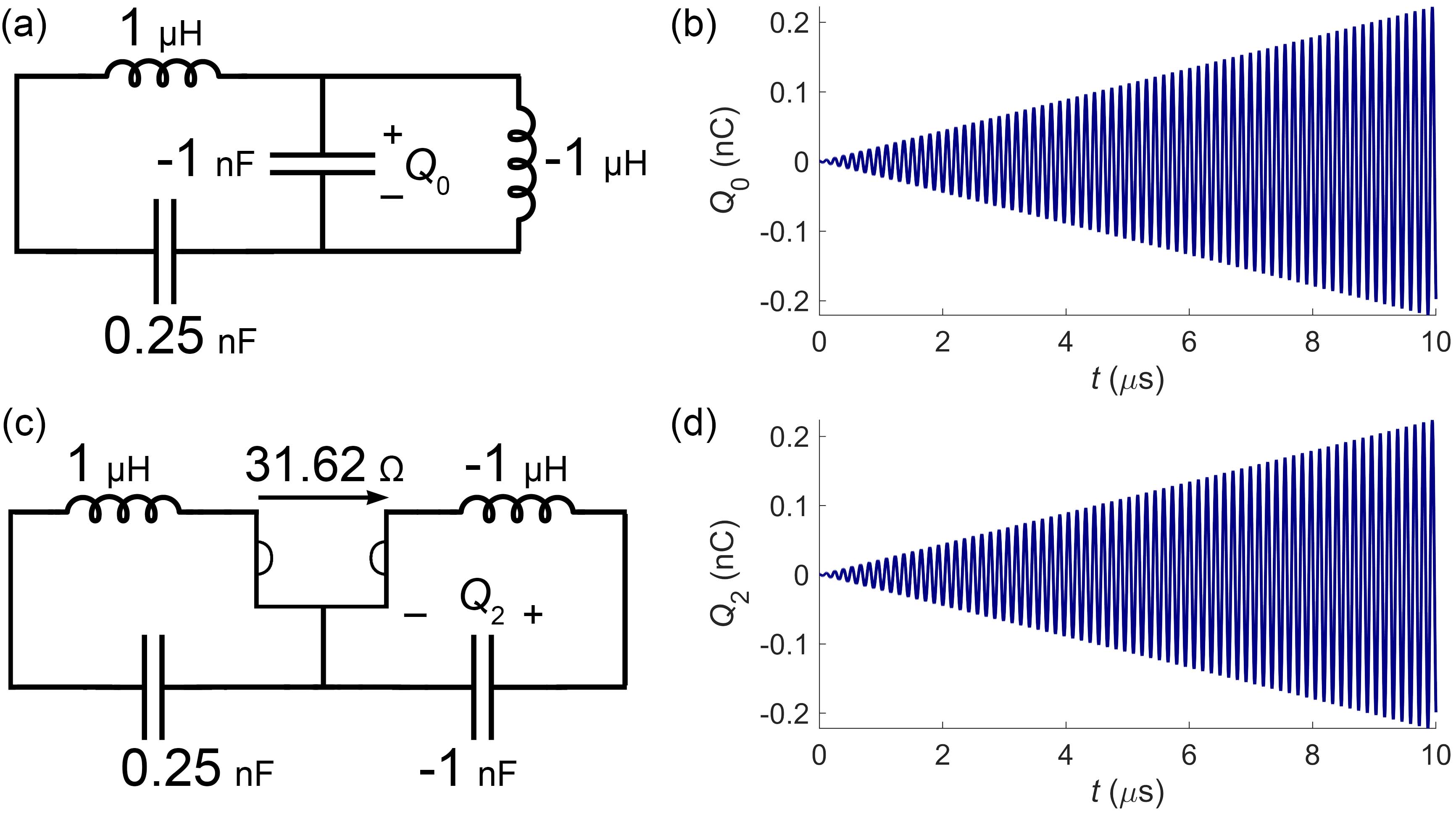
Figure 7. Comparison between the time-domain simulation results of (a) the PRC and (c) the GNC with the proposed equivalent element values. The stored charges in the capacitor with the negative capacitance in (b) the PRC $Q_{0}\left(t\right)$ and (d) the GNC $Q_{2}\left(t\right)$ under the EPD condition and by applying the equivalency conditions.

11. Conclusions

We have synthesized a conservative (lossless) electric circuit capable of attaining a nontrivial Jordan canonical form for its evolution matrix and consequently exhibiting an EPD. The circuit is composed of solely conservative reciprocal elements (capacitors and inductors) and the shared capacitance and parallel inductance should be negative. Interestingly, we found that the reciprocal and nonreciprocal circuits presented in our previous papers can produce exactly the same Jordan canonical form. We also found that the nonreciprocity is manifested in breakdown of the certain symmetry of the set of eigenvectors as well as in the Lagrangian. Further, we have thoroughly tested and confirmed all our significant findings using numerical simulation using commercial circuit simulator software.

A. Kirchoff’s Equations for The PRC

The following is a concise review of the fundamental equations of the circuit shown in Figure 3 based on Kirchhoff’s laws. According to Kirchhoff’s voltage law in the two fundamental loops of the PRC we have

$$\ddot{q}_{1}+\left(\frac{1}{L_{1}C_{1}}+\frac{1}{L_{1}C_{0}}\right)q_{1}-\left(\frac{1}{L_{1}C_{0}}\right)q_{0}=0,$$ (A.1a)

$$\ddot{q}_{0}-\left(\frac{1}{L_{0}C_{0}}\right)q_{1}+\frac{1}{L_{0}C_{0}}q_{0}=0.$$ (A.1b)

Then, the circuit vector evolution equation and the eigenvalue problem are expressed as

$$\partial_{t}\mathsf{q}_{\mathrm{r}}=\mathscr{C}\mathsf{q}_{\mathrm{r}},\quad\mathscr{C}_{\mathrm{r}}=\left[\begin{array}[]{rrcr}0&0&1&0\\ 0&0&0&1\\ -\left(\frac{1}{L_{1}C_{1}}+\frac{1}{L_{1}C_{0}}\right)&\frac{1}{L_{1}C_{0}}&0&0\\ \frac{1}{L_{0}C_{0}}&-\frac{1}{L_{0}C_{0}}&0&0\end{array}\right],\quad\mathsf{q}_{\mathrm{r}}=\left[\begin{array}[]{c}\mathrm{q}_{\mathrm{r}}\\ \partial_{t}\mathrm{q}_{\mathrm{r}}\end{array}\right],\quad\mathrm{q}_{\mathrm{r}}=\left[\begin{array}[]{c}q_{1}\\ q_{0}\end{array}\right],$$ (A.2)

which is in full agreement with circuit vector evolution equation calculated by the Euler-Lagrange formulation in Equation (4.4).

B. Basics of Electric Networks

As a matter of self-consistency, we provide here an overview of the basic concepts and notations of electrical network theory. Graph theory concepts of branches (edges), nodes (vertices) and their incidences are used in the construction of electrical network theory. The Kirchhoff current and voltage laws can be used in this approach, which is effective in loop analysis and selecting independent variables. Specifically, we are interested in conservative electrical networks, which are composed of three types of electric elements: capacitors, inductors, and gyrators [41]. Inductors and capacitors are two-terminal electric elements, while gyrators are four-terminal electric elements.

B.1. Current-voltage relation in the circuit elements

In this case, a capacitor, an inductor, a resistor, and a gyrator are the elements of the basic electric circuit. These elements are characterized by current-voltage relationships as follows [42, 43, 44, 45]:

$$i_{\mathrm{c}}=C\partial_{t}v_{\mathrm{c}},\quad v_{\mathrm{l}}=L\partial_{t}i_{\mathrm{l}},\quad v_{\mathrm{r}}=Ri_{\mathrm{r}},$$ (B.1)

where $i_{\mathrm{c}}$, $i_{\mathrm{l}}$ and $i_{\mathrm{r}}$ are currents and $v_{\mathrm{c}}$, $v_{\mathrm{l}}$ and $v_{\mathrm{r}}$ are voltages, and real $C$, $L$ and $R$ are called respectively the capacitance, the inductance and the resistance as shown in Figure 8.

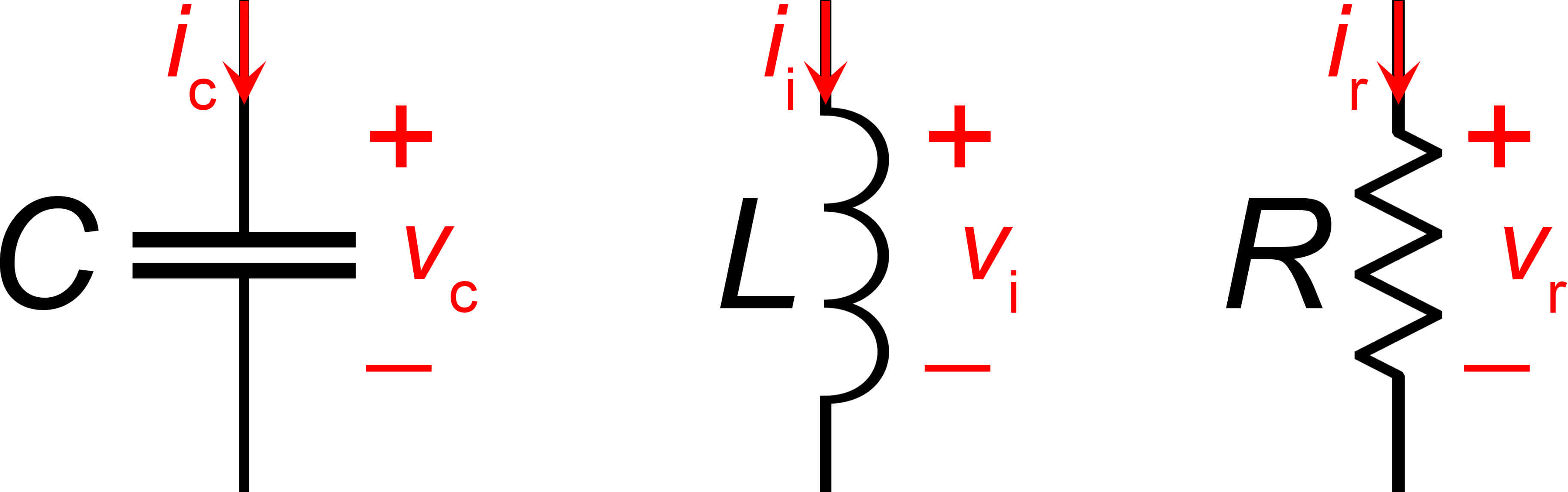
Figure 8. Capacitance, inductance and resistance symbols and the relevant parameters in the electric circuits.

In addition to the current and voltage we introduce the charge $q$ and the momentum $p$ as

$$q\left(t\right)=\intop i\left(t\right)\,dt,\quad i\left(t\right)=\partial_{t}q,$$ (B.2a)

$$p\left(t\right)=\intop v\left(t\right)\,dt,\quad v\left(t\right)=\partial_{t}p.$$ (B.2b)

Also, we describe the stored energy parameter $w$ for the elements. Then, the current-voltage-charge relations, the stored energy and the Lagrangians associated with the circuit elements are represented as [46, Chapter 3]

$$\text{Capacitor: }v_{\mathrm{c}}=\frac{q_{\mathrm{c}}}{C},\quad i_{\mathrm{c}}=\partial_{t}q_{\mathrm{c}}=C\partial_{t}v_{\mathrm{c}},\quad q_{\mathrm{c}}=Cv_{\mathrm{c}}=C\partial_{t}p_{\mathrm{c}},$$ (B.3a)

$$w_{\mathrm{c}}=\frac{1}{2}q_{\mathrm{c}}v_{\mathrm{c}}=\frac{1}{2}\frac{q_{\mathrm{c}}^{2}}{C}=\frac{1}{2}Cv_{\mathrm{c}}^{2}=\frac{1}{2}C\left(\partial_{t}p_{\mathrm{c}}\right)^{2},$$ (B.3b)

$$\mathcal{L}_{\mathrm{c}}=\frac{q_{\mathrm{c}}^{2}}{2C}.$$ (B.3c)

$$\text{Inductor: }v_{\mathrm{i}}=L\partial_{t}i_{\mathrm{i}},\quad p_{\mathrm{i}}=Li_{\mathrm{i}}=L\partial_{t}q_{\mathrm{i}},\quad\partial_{t}q_{\mathrm{i}}=\frac{p_{\mathrm{i}}}{L},$$ (B.3d)

$$w_{\mathrm{i}}=\frac{1}{2}p_{\mathrm{i}}i_{\mathrm{i}}=\frac{1}{2}Li_{\mathrm{i}}^{2}=\frac{1}{2}L\left(\partial_{t}q_{\mathrm{i}}\right)^{2}=\frac{1}{2}\frac{p_{\mathrm{i}}^{2}}{L},$$ (B.3e)

$$\mathcal{L}_{\mathrm{i}}=\frac{L\left(\partial_{t}q_{\mathrm{i}}\right)^{2}}{2}.$$ (B.3f)

$$\text{Resistor: }v_{\mathrm{r}}=Ri_{\mathrm{r}},\quad p_{\mathrm{r}}=Rq_{\mathrm{r}}.$$ (B.3g)

B.2. Negative impedance converter

Our circuits require negative capacitances and inductances, which can be provided by a number of physical devices. [47, Chapter 29]. Figure 9 shows suggested circuits that utilize operational amplifiers (opamps) to obtain negative impedance, capacitance and inductance [48, Chapter 10]. The voltage and current relation and input impedance for circuits depicted in Figure 9 are respectively as follows:

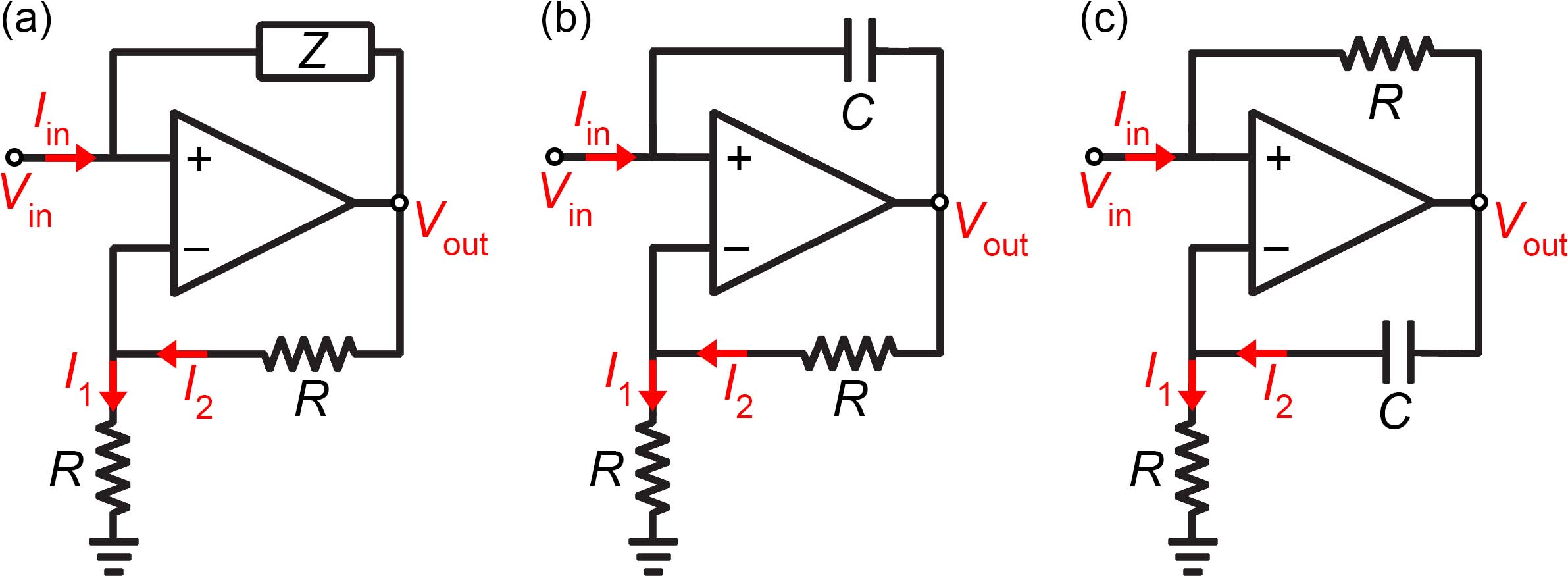
Figure 9. Opamp-based negative (a) impedance converter, (b) capacitance converter, (c) inductance converter.

(i) for the negative impedance converter (Figure 9(a)):

$$I_{1}=I_{2}=\frac{V_{\mathrm{in}}}{R},\quad V_{\mathrm{o}}=2V_{\mathrm{in}}\;\Rightarrow\;Z_{\mathrm{in}}=\frac{V_{\mathrm{in}}}{I_{\mathrm{in}}}=-Z;$$ (B.4)

(ii) for the negative capacitance converter(Figure 9(b)):

$$I_{1}=I_{2}=\frac{V_{\mathrm{in}}}{R},\quad V_{\mathrm{o}}=2V_{\mathrm{in}}\;\Rightarrow\;Z_{\mathrm{in}}=\frac{V_{\mathrm{in}}}{I_{\mathrm{in}}}=-\frac{1}{\mathrm{i}\omega C};$$ (B.5)

(iii) for the negative inductance converter (Figure 9(c)):

$$I_{1}=I_{2}=\frac{V_{\mathrm{in}}}{R},\quad V_{\mathrm{o}}=V_{\mathrm{in}}\left(1+\frac{1}{\mathrm{i}\omega RC}\right)\;\Rightarrow\;Z_{\mathrm{in}}=\frac{V_{\mathrm{in}}}{I_{\mathrm{in}}}=-\mathrm{i}\omega\left(R^{2}C\right).$$ (B.6)

There are limitations associated with any physical implementation of an opamp due to deviations from ideal assumptions. Most opamps deviate from ideal conditions as a result of their limited frequency band and frequency dependence. A proper tuning of the circuit elements can restore the EPD property at a single frequency, as the EPD occurs at a single frequency. It is important to note that the opamp-based circuits of impedance converters shown in Figure 9 are only examples; there are many other implementations with different features available.

C. Single LC Circuit Analysis

The circuit matrix of the single LC resonator is given by

$$\mathscr{C}_{\mathrm{LC}}=\left[\begin{array}[]{rr}0&-1\\ \omega_{0}^{2}&0\end{array}\right],\quad\omega_{0}=\frac{1}{\sqrt{LC}}$$ (C.1)

where $\omega_{0}$ is the resonance frequency of the single LC resonator. Then, the eigenvalues are expressed as $s_{1,2}=\pm\mathrm{i}\omega_{0}$ and the corresponding eigenvectors by assuming state vector as the stored charge in the capacitance $q$ and its first derivative, $\Psi_{\mathrm{LC}}=\left[q,\dot{q}\right]$, are obtained as

$$\mathscr{V}_{\mathrm{LC}}=\left[\begin{array}[]{rr}\frac{1}{2}&\frac{1}{2}\\ \mathrm{i}\frac{1}{2\sqrt{LC}}&-\mathrm{i}\frac{1}{2\sqrt{LC}}\end{array}\right]=\left[\begin{array}[]{rr}\frac{1}{2}&\frac{1}{2}\\ \mathrm{i}\frac{\omega_{0}}{2}&-\mathrm{i}\frac{\omega_{0}}{2}\end{array}\right].$$ (C.2)

We define impedance as a ratio between voltage ($v$) and current ($i$). Also, by using the definition of charge in the state vector which is defined based on the stored charge in the capacitance $q$, we calculate resonator impedance as a ratio between capacitor voltage ($q/C$) and capacitor current ($\dot{q}$) as

$$Z_{1,2}=\pm\frac{1}{\mathrm{i}\omega_{0}C},\quad\left|Z_{1,2}\right|=\sqrt{\frac{L}{C}},$$ (C.3)

which is defined as an impedance of single resonator.

D. List of Abbreviations

• EPD: exceptional point of degeneracy

• GNC: gyrator-based nonreciprocal circuit

• PRC: principle reciprocal circuit

Data Availability: The data that supports the findings of this study are available within the article.

Acknowledgment: This research was supported by Air Force Office of Scientific Research (AFOSR) Grant No. FA9550-19-1-0103.

References

- [1] T. Kato, Perturbation theory for linear operators. Springer Science & Business Media, 1966.
- [2] W. Heiss and A. Sannino, “Avoided level crossing and exceptional points,” Journal of Physics A: Mathematical and General, vol. 23, no. 7, p. 1167, 1990.
- [3] W. Heiss, “Exceptional points–their universal occurrence and their physical significance,” Czechoslovak Journal of physics, vol. 54, pp. 1091–1099, 2004.
- [4] T. Stehmann, W. Heiss, and F. Scholtz, “Observation of exceptional points in electronic circuits,” Journal of Physics A: Mathematical and General, vol. 37, no. 31, p. 7813, 2004.
- [5] W. Heiss, “The physics of exceptional points,” Journal of Physics A: Mathematical and Theoretical, vol. 45, no. 44, p. 444016, 2012.
- [6] W. Heiss, “Exceptional points of non-hermitian operators,” Journal of Physics A: Mathematical and General, vol. 37, no. 6, p. 2455, 2004.
- [7] J. Wiersig, “Enhancing the sensitivity of frequency and energy splitting detection by using exceptional points: application to microcavity sensors for single-particle detection,” Physical review letters, vol. 112, no. 20, p. 203901, 2014.
- [8] J. Wiersig, “Sensors operating at exceptional points: General theory,” Physical review A, vol. 93, no. 3, p. 033809, 2016.
- [9] W. Chen, Ş. Kaya Özdemir, G. Zhao, J. Wiersig, and L. Yang, “Exceptional points enhance sensing in an optical microcavity,” Nature, vol. 548, no. 7666, pp. 192–196, 2017.
- [10] C. M. Bender and S. Boettcher, “Real spectra in non-hermitian hamiltonians having p t symmetry,” Physical review letters, vol. 80, no. 24, p. 5243, 1998.
- [11] H. Ramezani, T. Kottos, R. El-Ganainy, and D. N. Christodoulides, “Unidirectional nonlinear pt-symmetric optical structures,” Physical Review A, vol. 82, no. 4, p. 043803, 2010.
- [12] I. Barashenkov, D. Pelinovsky, and P. Dubard, “Dimer with gain and loss: Integrability and-symmetry restoration,” Journal of Physics A: Mathematical and Theoretical, vol. 48, no. 32, p. 325201, 2015.
- [13] M. A. Othman and F. Capolino, “Demonstration of a degenerate band edge in periodically-loaded circular waveguides,” IEEE Microwave and Wireless Components Letters, vol. 25, no. 11, pp. 700–702, 2015.
- [14] M. Y. Nada, M. A. Othman, and F. Capolino, “Theory of coupled resonator optical waveguides exhibiting high-order exceptional points of degeneracy,” Physical Review B, vol. 96, no. 18, p. 184304, 2017.
- [15] M. Y. Nada, T. Mealy, and F. Capolino, “Frozen mode in three-way periodic microstrip coupled waveguide,” IEEE Microwave and Wireless Components Letters, vol. 31, no. 3, pp. 229–232, 2020.
- [16] T. Mealy and F. Capolino, “General conditions to realize exceptional points of degeneracy in two uniform coupled transmission lines,” IEEE Transactions on Microwave Theory and Techniques, vol. 68, no. 8, pp. 3342–3354, 2020.
- [17] A. Herrero-Parareda, I. Vitebskiy, J. Scheuer, and F. Capolino, “Frozen mode in an asymmetric serpentine optical waveguide,” Advanced Photonics Research, vol. 3, no. 9, p. 2100377, 2022.
- [18] J. Schindler, A. Li, M. C. Zheng, F. M. Ellis, and T. Kottos, “Experimental study of active lrc circuits with pt symmetries,” Physical Review A, vol. 84, no. 4, p. 040101, 2011.
- [19] J. Schindler, Z. Lin, J. M. Lee, H. Ramezani, F. M. Ellis, and T. Kottos, “Pt-symmetric electronics,” Journal of Physics A: Mathematical and Theoretical, vol. 45, p. 444029, oct 2012.
- [20] H. Hodaei, A. U. Hassan, S. Wittek, H. Garcia-Gracia, R. El-Ganainy, D. N. Christodoulides, and M. Khajavikhan, “Enhanced sensitivity at higher-order exceptional points,” Nature, vol. 548, no. 7666, pp. 187–191, 2017.
- [21] H. Kazemi, M. Y. Nada, T. Mealy, A. F. Abdelshafy, and F. Capolino, “Exceptional points of degeneracy induced by linear time-periodic variation,” Physical Review Applied, vol. 11, no. 1, p. 014007, 2019.
- [22] K. Rouhi, H. Kazemi, A. Figotin, and F. Capolino, “Exceptional points of degeneracy directly induced by space–time modulation of a single transmission line,” IEEE Antennas and Wireless Propagation Letters, vol. 19, no. 11, pp. 1906–1910, 2020.
- [23] H. Kazemi, M. Y. Nada, A. Nikzamir, F. Maddaleno, and F. Capolino, “Experimental demonstration of exceptional points of degeneracy in linear time periodic systems and exceptional sensitivity,” Journal of Applied Physics, vol. 131, no. 14, p. 144502, 2022.
- [24] A. Nikzamir, K. Rouhi, A. Figotin, and F. Capolino, “Time modulation to manage and increase the power harvested from external vibrations,” Applied Physics Letters, vol. 123, p. 211701, 11 2023.
- [25] A. Figotin, “Synthesis of lossless electric circuits based on prescribed jordan forms,” Journal of Mathematical Physics, vol. 61, no. 12, p. 122703, 2020.
- [26] A. Figotin, “Perturbations of circuit evolution matrices with jordan blocks,” Journal of Mathematical Physics, vol. 62, no. 4, p. 042703, 2021.
- [27] A. Nikzamir, K. Rouhi, A. Figotin, and F. Capolino, “Demonstration of exceptional points of degeneracy in gyrator-based circuit for high-sensitivity applications,” arXiv preprint arXiv:2107.00639, 2021.
- [28] K. Rouhi, A. Nikzamir, A. Figotin, and F. Capolino, “Exceptional point in a degenerate system made of a gyrator and two unstable resonators,” Physical Review A, vol. 105, no. 3, p. 032214, 2022.
- [29] K. Rouhi, A. Nikzamir, A. Figotin, and F. Capolino, “High-sensitivity in various gyrator-based circuits with exceptional points of degeneracy,” EPJ Applied Metamaterials, vol. 9, p. 8, 2022.
- [30] A. Nikzamir, K. Rouhi, A. Figotin, and F. Capolino, “How to achieve exceptional points in coupled resonators using a gyrator or pt-symmetry, and in a time-modulated single resonator: high sensitivity to perturbations,” EPJ Applied Metamaterials, vol. 9, p. 14, 2022.
- [31] B. D. Tellegen, “The gyrator, a new electric network element,” Philips Res. Rep, vol. 3, no. 2, pp. 81–101, 1948.
- [32] J. Helszajn, Microwave engineering: passive, active, and non-reciprocal circuits. McGraw-Hill, New York,, 1992.
- [33] A. Figotin and I. Vitebsky, “Spectra of periodic nonreciprocal electric circuits,” SIAM Journal on Applied Mathematics, vol. 61, no. 6, pp. 2008–2035, 2001.
- [34] F.-Y. Wu, “Theory of resistor networks: the two-point resistance,” Journal of Physics A: Mathematical and General, vol. 37, no. 26, p. 6653, 2004.
- [35] N. S. Izmailian, R. Kenna, and F. Wu, “The two-point resistance of a resistor network: a new formulation and application to the cobweb network,” Journal of Physics A: Mathematical and Theoretical, vol. 47, no. 3, p. 035003, 2013.
- [36] A. Seyranian, O. Kirillov, and A. Mailybaev, “Coupling of eigenvalues of complex matrices at diabolic and exceptional points,” Journal of Physics A: Mathematical and General, vol. 38, no. 8, p. 1723, 2005.
- [37] H. Cartarius, D. Haag, D. Dast, and G. Wunner, “Nonlinear schrödinger equation for a-symmetric delta-function double well,” Journal of Physics A: Mathematical and Theoretical, vol. 45, no. 44, p. 444008, 2012.
- [38] R. Gutöhrlein, J. Main, H. Cartarius, and G. Wunner, “Bifurcations and exceptional points in dipolar bose–einstein condensates,” Journal of Physics A: Mathematical and Theoretical, vol. 46, no. 30, p. 305001, 2013.
- [39] R. Gutöhrlein, H. Cartarius, J. Main, and G. Wunner, “Bifurcations and exceptional points in a-symmetric dipolar bose–einstein condensate,” Journal of Physics A: Mathematical and Theoretical, vol. 49, no. 48, p. 485301, 2016.
- [40] A. P. Seyranian and A. A. Mailybaev, Multiparameter stability theory with mechanical applications, vol. 13. World Scientific, 2003.
- [41] W. Tzeng and F. Wu, “Theory of impedance networks: the two-point impedance and lc resonances,” Journal of Physics A: Mathematical and General, vol. 39, no. 27, p. 8579, 2006.
- [42] W. Cauer, Synthesis of linear communication networks, vol. 1. McGraw-Hill, 1958.
- [43] N. Balabanian and T. A. Bickart, Electrical network theory. John Wiley & Sons, 1969.
- [44] W. H. Hayt and G. W. Neudeck, Electronic circuit analysis and design. Houghton Mifflin Company, 1984.
- [45] J. D. Irwin and R. M. Nelms, Basic engineering circuit analysis. John Wiley & Sons, 2020.
- [46] P. I. Richards, Manual of mathematical physics. Macmillan, 1959.
- [47] R. C. Dorf, The engineering handbook. CRC press, 2018.
- [48] A. Izadian, Fundamentals of Modern Electric Circuit Analysis and Filter Synthesis. Springer, 2023.