On the QCD critical point, Lee-Yang edge singularities and Padé resummations

Abstract

We analyze the trajectory of the Lee-Yang edge singularities of the QCD equation of state in the complex baryon chemical potential ($\mu_{B}$) plane for different values of the temperature by using the recent lattice results for the Taylor expansion coefficients up to eighth order in $\mu_{B}$ and various resummation techniques that blend in Padé expansions and conformal maps. By extrapolating from this information, we estimate for the location of the QCD critical point, $T_{c}\approx 100$ MeV, $\mu_{c}\approx 580$ MeV. We also estimate the crossover slope at the critical point to be $\alpha_{1}\approx 9^{\circ}$ and further constrain the non-universal mapping parameters between the three-dimensional Ising model and QCD equations of state.

I Introduction

Mapping the phase diagram of Quantum Chromodynamics (QCD) for different temperatures and baryon densities, probed by the baryon chemical potential, $\mu_{B}$, is currently one of the major open problems in nuclear physics. The state-of-the-art lattice simulations provide a lot of information about the thermodynamic properties for vanishing chemical potential. For example it is well established that the transition between the baryonic phase and quark-gluon plasma is a smooth crossover Aoki:2006we . However, at finite chemical potential, the applicability of lattice QCD is severely limited due to the fermion sign problem (for reviews see e.g. Refs. Philipsen:2007aa ; deForcrand:2009zkb ; Ding:2015ona ). One of the central questions regarding the QCD phase diagram at finite temperature and chemical potential is whether there is a second order critical point, and a first-order transition curve emanating from it Bzdak:2019pkr . From the experimental perspective, this question has been the main motivation behind the Beam Energy Scan program at the Relativistic Heavy Ion Collider as well as the future Compressed Baryonic Matter experiment at Facility for Antiproton and Ion Research Almaalol:2022xwv .

From the theoretical standpoint, the first principle computations of the QCD phase diagram at finite chemical potential requires tackling the fermion sign problem in some way. The two main approaches that bypass the sign problem are Taylor expanding around $\mu_{B}=0$ Allton:2002zi , and performing lattice simulations at pure imaginary chemical potential and analytically continuing from it deForcrand:2002hgr ; DElia:2002tig ; Bellwied:2015rza ; Ratti:2018ksb ; Borsanyi:2021sxv . In the former approach, one expands the equation of state in $\mu_{B}$ as a Taylor series whose coefficients are observables evaluated at $\mu_{B}=0$ which can be computed without a sign problem. At the same time, even in the absence of the fermion sign problem, the computation of the higher order Taylor coefficients on the lattice become progressively more difficult due to noise. The state-of-the-art computations go up to ${\cal O}({\mu_{B}^{8}})$ (for recent results see HotQCD Bollweg:2022rps ; Bollweg:2022fqq and Wuppertal-Budapest Borsanyi:2020fev collaborations). Currently, based on the available data, an existence of a critical point for $\mu_{B}/T\lesssim 3$ is highly disfavored.

Even with having access to a modest number Taylor coefficients, it is possible extract useful information regarding the equation of state that goes beyond approximating it as a truncated Taylor expansion. The starting point is that, for any temperature, the equation of state possess singularities for complex values of $\mu_{B}^{2}$, the Lee-Yang (LY) edge singularities. With certain assumptions regarding location of the nearest singularity to origin, $\mu_{B}=0$, one could estimate the location of the singularity from the Taylor coefficients. Furthermore, in the vicinity of a critical point, the LY singularities obey a particular scaling form. The key idea is to map the extrapolated singularity from the Taylor coefficients at different temperatures, which we shall call the “Lee-Yang trajectory”, and compare it with the scaling form predicted by critical scaling. This way, one can push the information extracted from the Taylor coefficients beyond the region constrained by the truncated expansion. The idea of extracting the location of LY singularities from the truncated Taylor expansion goes back to work of Fisher Fisher:1974series . The significance of the LY trajectory in the context of the QCD phase diagram and the critical point has been pointed out in Halasz_1997 ; Ejiri:2005ts ; Stephanov:2006dn . Recently, based on these observations, quantitative estimations of the LY trajectory by extracting the radius of convergence or using Padé type resummations have been made Mukherjee:2019eou ; Connelly:2020pno ; Basar:2021hdf ; Basar:2021gyi ; Dimopoulos:2021vrk ; Nicotra:2021ijp ; Singh:2021pog ; Schmidt:2022ogw ; Bollweg:2022rps ; Clarke:2023noy ; Bollweg:2022fqq .

In this paper, we utilize an efficient method that improves Padé resummation in order to construct the LY trajectory. We use the recent HotQCD collaboration results Bollweg:2022rps ; Bollweg:2022fqq for the Taylor coefficients. From the improved resummation, assuming that the trajectory, in part, can be captured by the scaling behavior of the critical point, we extrapolate the location of the critical point and constrain the critical contribution to the equation of state in its vicinity. This is our main result and is summarized in Table 1 in Section IV. Our hope is that these results can be incorporated into the state-of-the-art parameterizations of the equation of state such as in Refs. Parotto:2018pwx ; An:2021wof in to order to assist the experimental effort for the search for the critical point.

The rest of the paper is organized as follows. In Sec. II we summarize the physics of LY singularities in the context of the QCD critical point and establish the notation that we use for the rest of the paper. In Sec. III, we build the necessary mathematical machinery that we use to extract the singularities from the Taylor coefficients. Our results are presented in Sec. IV. We extensively discuss these results in the final section, Sec. V.

II Lee-Yang edge singularities

In their seminal work in 1952, Lee and Yang showed that phase transitions of a thermodynamic system can be understood in terms of the complex singularities of the grand canonical partition function Yang:1952be ; Lee:1952ig . In general, the partition function, $Z(\zeta)$, of a system with finitely many degrees of freedom is a polynomial in fugacity, $\zeta=e^{\mu/T}$, and is nonnegative for $\zeta>0$. Of course, being a polynomial, it has zeroes for complex values of $\zeta$, which, in the thermodynamic limit, coalesce into branch points that emanate from the so called Lee-Yang edge singularities. At a second order phase transition the LY edge singularities pinch the real axis.

We shall focus on the LY singularities associated with the three Ising model which belongs to the same universality class as QCD. In the Ising model, there are two relevant operators, energy density and spin, whose couplings are the reduced temperature, $r$, and the magnetic field, $h$. The critical point in the phase diagram sits at $r=h=0$. The transition between positive and negative magnetization phases (probed by $h>0$ and $h<0$ respectively) is a smooth crossover for $r>0$ and a first order transition for $r<0$. It is convenient to use the scaling variable $x=hr^{-{\beta\delta}}$ to express the location the LY singularity which is simply along the pure imaginary axis:

$$x=\pm ix_{LY}\,.$$ (1)

Here $\beta$ and $\delta$ are the usual Ising critical exponents ZinnJustin:2002ru . In this work we use the value computed from conformal bootstrap PhysRevD.86.025022

$${\beta\delta}\approx 1.5631\,.$$ (2)

The value of $x_{LY}$ has been recently computed via functional renormalization group Rennecke:2022ohx ; Connelly:2020gwa ; Johnson:2022cqv as well as using the Schofield representation Karsch:2023rfb . Based on these works we will use the value:

$$x_{LY}=|z_{c}|^{-{\beta\delta}}\approx 0.246$$ (3)

The LY singularity is a critical point as well and the equation of state in its vicinity belongs to the same universality class as the $\phi^{3}$ theory with a pure imaginary coupling Fisher:1978pf . The universal, singular contribution to the magnetization around the LY singularity is given by

$$m-m_{c}\sim(x\pm ix_{LY})^{\sigma_{LY}}$$ (4)

with the critical exponent $\sigma_{LY}\approx 0.074-0.085$ An:2016lni . For a more detailed analysis of the analytical structure of the LY singularities in three and two-dimensional Ising models we refer the reader to Refs. An:2016lni ; An:2017brc and Fonseca:2001dc respectively. In the latter case, the physics of the LY singularity is captured by a non-unitary conformal field theory. In the former case, an analogous analytical construction does not exist at the moment, and one has to rely on numerical results such as the epsilon expansion.

The above observations about the three-dimensional Ising model can now be translated into QCD, given that these two theories are in the same universality class. In the vicinity of the critical point, $(T_{c},\mu_{c})$, the relevant directions in the QCD phase diagram, $T$ and $\mu_{B}$, can be mapped to those of the Ising model, $h$ and $r$, via a linear map Parotto:2018pwx ; Pradeep:2019ccv

$$\begin{pmatrix}r\\ h\end{pmatrix}:=\begin{pmatrix}r_{T}&&h_{T}\\ r_{\mu}&&h_{\mu}\end{pmatrix}\begin{pmatrix}T-T_{c}\\ \mu-\mu_{c}\end{pmatrix}.\quad$$ (5)

This mapping then leads to the following expression for the trajectory of the LY singularities of QCD in the vicinity of the critical point Stephanov:2006dn :

$$\mu_{LY}(T)\approx\mu_{c}-c_{1}(T-T_{c})\pm ix_{LY}c_{2}(T-T_{c})^{\beta\delta},$$

$$\text{where }c_{1}:={{h_{T}}\over{h_{\mu}}}:=\tan\alpha_{1}\quad c_{2}:={{r_{\mu}}^{\beta\delta}\over{h_{\mu}}}\left({{r_{T}}\over{r_{\mu}}}-{{h_{T}}\over{h_{\mu}}}\right)^{{\beta\delta}}.\quad$$ (6)

Notice that $c_{1}$ is the slope of the crossover line, whereas $c_{2}$ depends on the relative angle, $\alpha_{2}$, between the $h$ and $r$ axes Parotto:2018pwx ; Pradeep:2019ccv . Remarkably the trajectory in Eq. (II) depends not only on the location of the critical point, but also on the non-universal mapping parameters. Our goal is to reconstruct Eq. (II) and constrain these non-universal values from the Taylor series coefficients of the equation of state.

III Resummations and conformal maps

Our aim is to extract the singular behavior of the equation of state $p(T,\mu_{B})$ from its Taylor series expansion around $\mu_{B}=0$,

$$\frac{p(T,\mu_{B})-p(T,0)}{T^{4}}\approx\sum_{n=0}^{N}\frac{\chi_{2n}(T)}{(2n)!}\left(\mu_{B}\over T\right)^{2n}\,.$$ (7)

Of course, in practice we only have access to a finitely many terms, and the truncated Taylor series is a polynomial which obviously has no singularities. However even with finitely many coefficients, one could extract the singular behavior of the equation of state. Assuming that the nearest singularity to the origin is the LY singularity, following the extended analyticity conjecture of Fonseca and Zamalodchikov Fonseca:2001dc , along with Darboux’s theorem, it is possible to estimate both $|\mu_{LY}|$ via the radius of convergence by using the standard root/ratio tests Bazavov:2017dus ; GIORDANO2021121986 ; Mukherjee:2019eou , as well as $\arg\mu_{LY}$ Basar:2021hdf ; Basar:2021gyi . However, since in our case the leading singularity is in fact a complex conjugate pair (see Eq. (II)), the roots/ratios of the coefficients exhibit oscillatory behavior due to interference between the phases of the two singularities which render these estimations numerically challenging.

A better approach is to use Padé resummation, which approximates the original function, $p(\mu_{B}^{2})$, by a rational function,

$${\rm P}[p](\mu_{B}^{2}):=\frac{q_{1}(\mu_{B}^{2})}{q_{2}(\mu_{B}^{2})}$$ (8)

where $p_{1}$ and $p_{2}$ are polynomials of order $[N/2]$, whose coefficients are determined by Taylor expanding ${\rm P_{N/2}}[p](\mu_{B}^{2})$ and matching the coefficients with the original ones in Eq. (7). The underlying singularities of $p(\mu_{B}^{2})$ are then represented by accumulation points the poles and zeroes of ${\rm P}[p](\mu_{B}^{2})$. Furthermore, if the underlying singularity is a branch point, the poles/zeroes lie on curved arcs. Remarkably, the shapes of these arcs can be understood in terms of a two-dimensional electrostatic problem of finding a configuration of charges (poles and zeroes) which minimizes an effective capacitance STAHL1997139 ; saff ; Costin:2020pcj . At the same time, in our case, where there is a complex conjugate pair of singularities, the arcs that emerge from each singularity coalesce along the real axis. These singularities along the real axis are unphysical, but they are not numerical artifacts; their existence is unavoidable with Padé resummation. To make things worse, their number grows as $N$ increases, limiting the applicability of the Padé resummation to $\mu\lesssim|\mu_{LY}|$.

In order to overcome this inherent shortcoming of Padé resummation, the next step we take is to pair it with a conformal map. In a way, Padé resummation already introduces its own conformal map by representing the branches with the curved arcs that minimize the effective capacitance. We can further improve the convergence properties of Padé, and extend it’s domain of applicability by using an additional conformal map. The idea is to map the complex $\mu_{B}^{2}$ plane, where the equation of state is expressed in, to a different (preferably compact) region, such as the unit disk. We will denote this new region as $\zeta$. In other words, we consider the conformal map:

$$\mu_{B}^{2}:=\phi(\zeta)\,.$$ (9)

We then expand the equation of state as a series expansion in $\zeta$ and perform the Padé resummation for this expansion:

$${\rm CP}[p](\zeta):=\frac{\tilde{q}_{1}(\zeta)}{\tilde{q}_{2}(\zeta)}\,.$$ (10)

where $\tilde{p}$ and $\tilde{q}$ are order $N/2$ polynomials whose coefficients are determined by the Taylor coefficients of $p(\phi(\zeta))$. We shall call this resummation simply as “conformal Padé”. Different choices of the conformal map, $\phi$, leads to significant improvements over the usual Padé resummation. Moreover, extra information such as the singular behavior of the original function can be “baked in” into the resummation via choosing an appropriate conformal map. Note that, in contrast, the only information that goes into Padé resummation is the Taylor coefficients. After performing the Padé resummation in the $\zeta$ plane, the original function is then represented as

$$f(\mu_{B}^{2})\underset{\text{conf. Pad\'{e}}}{=}{\rm CP}[p](\zeta)\big{|}_{\zeta=\phi^{-1}(\mu_{B}^{2})}\,.$$ (11)

For certain conformal maps, an analytical expression for the inverse function exists, and for others it does not and the inversion has to be computed numerically. Similar to Padé, the original singularities of the function are represented by accumulation of zeroes and poles of conformal Padé in $\zeta$ plane. They can be mapped back to $\mu_{B}^{2}$ plane via $\phi(\zeta)$. Note that the computation of the singularities does not require the inverse function. The key point is that for the conformal maps that we consider, the spurious poles appear outside the unit disk and therefore are not present in the $\mu_{B}^{2}$ plane Costin:2020hwg ; Costin:2021bay . We now discuss the conformal maps that we employ in this work.

The first map we use, which we name as the “two-cut map”, is defined as

$$\phi_{2}(\zeta)=4|\mu^{2}_{LY}|\left[\frac{\theta/\pi}{(1-\zeta)^{2}}\right]^{\theta/\pi}\left[\frac{1-\theta/\pi}{(1+\zeta)^{2}}\right]^{1-\theta/\pi}\,.$$ (12)

It maps the complex plane $\mu_{B}^{2}$ plane with two radial cuts into the unit disk as shown in Fig. 1. The branch points, located at $\mu_{B}^{2}:=|\mu_{LY}^{2}|e^{\pm i\theta}$ , are mapped to the edge of the unit disk with the angle $\psi_{2}:=2\arcsin(\sqrt{\theta/\pi})$:

$$|\mu_{LY}^{2}|e^{\pm i\theta}\rightarrow\zeta_{LY}=e^{\pm i\psi_{2}}$$ (13)

and the branch cuts are mapped to the edge of the unit disk as show in Fig. 1. Notably, this map has been used in other physical applications, mostly within the context of extracting the Borel singularities associated with asymptotic series Guida:1998bx ; Rossi:2018 ; Serone:2019szm ; Costin:2020hwg ; Costin:2021bay . As opposed to Padé, conformal Padé with the two-cut map does not generate unphysical poles along the real axis, allowing one to reconstruct the original function beyond the radius of convergence. Furthermore it generally gives a better estimate for the location of the branch singularities compared to Padé with the same number of Taylor coefficients Costin:2020pcj . One shortcoming of the two-cut map, however, is that its applicability is limited to the first Riemann sheet. Namely even though it gives a good estimate for the location of the branch singularities, it does not allow one to go pass the branch cuts. This can be seen from the fact that it maps the first Riemann sheet, bounded with the radial branch cuts, inside the whole unit disk.

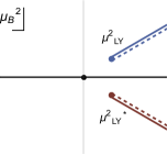
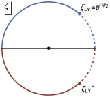
Figure 1: The original $\mu_{B}^{2}$ plane (right) with radial cuts and its image in the unit circle (right) under the two-cut map defined in Eq. (12).

An improvement over the two-cut map is the “uniformizing map” defined as

$$\phi_{u}(\tau)=|\mu^{2}_{LY}|\left(e^{-i\theta}+2i\sin\theta\lambda\left(\tau\right)\right)\,.$$ (14)

Here $\lambda(\tau)=\theta_{2}^{4}(\tau)/\theta_{3}^{4}(\tau)$ is the modular lambda function with $\theta_{2}(\tau)=\sum_{n=\infty}^{\infty}e^{2\pi i\tau(n+1/2)^{2}}$ and $\theta_{3}(\tau)=\sum_{n=\infty}^{\infty}e^{2\pi i\tau n^{2}}$ being the usual Jacobi elliptic functions defined in the upper half plane ${\rm Im}\tau>0$. We further map the upper half-plane into the unit disk via the following Mobius transformation:

$$\tau\rightarrow\tau(\zeta)=i\frac{\mathbb{K}\left(\frac{1}{2}-\frac{i}{2}\cot\theta\right)+\mathbb{K}\left(\frac{1}{2}+\frac{i}{2}\cot\theta\right)i\zeta}{\mathbb{K}\left(\frac{1}{2}+\frac{i}{2}\cot\theta\right)-\mathbb{K}\left(\frac{1}{2}-\frac{i}{2}\cot\theta\right)i\zeta}$$ (15)

where $\mathbb{K}(m)$ is the complete elliptic integral of the first kind:

$$\mathbb{K}(m)=\int_{0}^{\pi/2}\frac{d\theta}{\sqrt{1-m\sin^{2}\theta}}\,.$$ (16)

This map uniformizes the multi-sheeted $\mu_{B}^{2}$ plane of the original function by mapping the entire multi-sheeted domain into a simply connected domain. A path that crosses the branch cuts in the $\mu_{B}^{2}$ plane is represented by a smooth curve in the mapped plane. Let us briefly explain how this works in two steps.

The first step is to map the $\mu_{B}^{2}$ plane with vertical branches into the fundamental domain via Eq. (14). This map is shown in Fig. 2 (center). Notice that the entire $\mu_{B}^{2}$ is mapped into a subset of the upper half-plane, the fundamental domain. The remaining half-circular “gaps” are filled by Schwartz reflection of the fundamental domain. These reflections are transformations built out of the elementary modular transformations, $S:\tau-\rightarrow-1/\tau$ and $T:\tau\rightarrow\tau+1$. Each Schwartz reflection fills in a portion of the semi-circular gaps in the upper half-plane, a process that can in principle continued ad-infinitum, asymptotically filling the whole gap. These regions are the images of the higher Riemann sheets with each Schwartz reflection corresponding to a particular sheet. Therefore passing across different sheets in the $\mu_{B}^{2}$ plane is simply represented by moving smoothly in the $\tau$ plane. Each Schwarz reflection generates a progressively smaller region in the $\tau$ plane, therefore in order to resolve the higher sheets one needs progressively more precise information, meaning more Taylor coefficients.

The second step is to map the fundamental domain into the unit disk via the Mobius transformation given in Eq. (15). As seen in Fig. 2 (right), the branch points are mapped to the edge of the unit disk. Similar to the two-cut case, the angle is given by

$$|\mu_{LY}^{2}|e^{\pm i\theta}\rightarrow\zeta_{LY}=i\frac{\mathbb{K}\left(\frac{1}{2}\mp\frac{i}{2}\cot\theta\right)}{\mathbb{K}\left(\frac{1}{2}\pm\frac{i}{2}\cot\theta\right)}:=e^{\pm i\psi_{u}}$$ (17)

The branches, however are mapped into certain curves that for a boundary of a compact domain within the unit circle. This compact, skewed diamond shaped region bounded by these curves is image of the first sheet. The remaining gaps in the unit circle are filled with Mobius transformations of the Schwartz reflected regions in the modular $\tau$ plane. These are the images of higher sheets. Consequently the entire multi sheeted $\mu_{B}^{2}$ space is mapped into the unit circle and crossing between is represented by smooth paths within the unit circle.

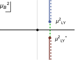
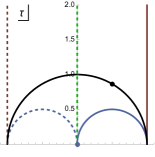
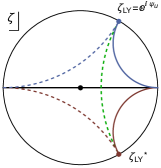
Figure 2: The original $\mu_{B}^{2}$ plane (right) with vertical cuts and its image in the modular $\tau$ plane (center) and the unit circle (right) under the uniformizing map defined in Eqs. (14) and (15).

This way, one can reconstruct the original function not only beyond its radius of convergence, but also in the higher Riemann sheets, just by using the Taylor coefficients of the expansion around the origin in the first Riemann sheet. In our context, the higher Riemann sheets encode the scaling equation of state in the first order phase transition region, $T<T_{c}$. In Ref. Basar:2021gyi we demonstrated this by reconstructing the equation of state of the mean field Ising model in the first-order transition region ($T<T_{c}$) by using the Taylor expansion coefficients of the high-temperature ($T>T_{c}$) equation of state obtained in the first Riemann sheet. In addition to reconstructing the equation of state in the higher sheets, the uniformizing map also provides a better approximation to the function compared to Padé and two-cut conformal Padé.

In this work, we will stick with the first sheet and use the uniformizing map to get a better estimate for the LY singularities and the equation of state. This is because we only have access to four Taylor coefficients with sizable statistical uncertainties which make the analytical continuation to higher sheets challenging. As opposed to the two-cut map, there is an analytical expression for the inverse of the uniformizing map, given as

$$\phi_{uni}^{-1}(\mu_{B}^{2})=-i\frac{\mathbb{K}\left(\kappa_{+}\right)\mathbb{K}\left(\kappa_{-}+\frac{i}{2\sin\theta}\frac{\mu^{2}_{B}}{|\mu^{2}_{LY}|}\right)-\mathbb{K}\left(\kappa_{-}\right)\mathbb{K}\left(\kappa_{+}-\frac{i}{2\sin\theta}\frac{\mu^{2}_{B}}{|\mu^{2}_{LY}|}\right)}{\mathbb{K}\left(\kappa_{-}\right)\mathbb{K}\left(\kappa_{-}+\frac{i}{2\sin\theta}\frac{\mu^{2}_{B}}{|\mu^{2}_{LY}|}\right)+\mathbb{K}\left(\kappa_{+}\right)\mathbb{K}\left(\kappa_{+}-\frac{i}{2\sin\theta}\frac{\mu^{2}_{B}}{|\mu^{2}_{LY}|}\right)}$$ (18)

where $\kappa_{\pm}:=(1\pm i\cot\theta)/2$ and $\theta=|\arg\mu^{2}_{LY}|$.

Notice that both the two-cut map and the uniformizing map depend on the location of the singularity, $\mu_{LY}$. Of course, a priori, we do not have this information. In fact, it is precisely this information we would like to extract by using these resummation techniques. The procedure we employ to overcome this seemingly paradoxical situation is simple. We first guess the location from ordinary Padé and use this initial guess as the value of $\mu_{LY}$ in the conformal map. Then we extract the poles from conformal Padé in $\zeta$ plane whose images in the $\mu_{B}^{2}$ plane gives us a refined estimate for $\mu_{LY}$. Now we iterate the same procedure by using this refined estimate for the value of $\mu_{LY}$ in the conformal map and repeating the same steps. We have observed that this iteration converges to a value which is our final estimate for $\mu_{LY}$. We finally repeat this iterative process for different temperatures to construct the LY trajectory.

Before presenting our results we briefly comment on an alternative resummation technique. The equation of state in the vicinity of the LY singularities has a singular contribution, but this singular contribution actually vanishes at the singularity for the pressure and generates a cusp for the density. However a true divergence occurs for the susceptibility. Of course, for real values of $\mu_{B}$ and $T>T_{c}$, the susceptibility does not diverge but peaks around ${\rm Re}\mu_{LY}$. For this reason, sometimes performing a Padé resummation for the susceptibility instead of the pressure can give a better estimate of the underlying singularities as well as the function itself. Therefore we also performed resummation for the susceptibility:

$$\chi(T,\mu_{B})={\partial^{2}p\over\partial\mu_{B}^{2}}\approx\sum_{n=0}^{N-1}\frac{\chi_{2n+2}(T)}{(2n)!}\left(\mu_{B}\over T\right)^{2n}\,.$$ (19)

Of course, using pressure or susceptibility in the resummation just amounts to reshuffling the same Taylor coefficients. However this reshuffling, especially when $N$ is small, does make a difference. For example in Refs. Basar:2021hdf ; Basar:2021gyi where we studied the Gross-Neveu and the Chiral Random Matrix models, using the susceptibility lead to much more accurate results than the pressure. For QCD we found that the situation is more complicated due to the statistical uncertainties in the coefficients as we discuss further in the next section .

IV Results

In this section we present our results for estimates for the Lee-Yang singularities as a function of temperature, obtained using the resummation methods described above. By using this estimate we then extrapolate the location of the critical point and the non-universal mapping parameters between Ising and QCD equations of state given in Eq. (5). We also present results for the susceptibility as a function of chemical potential for a few different temperatures.

We use the recent results for the Taylor coefficients up to ${\cal O}(\mu_{B}^{8})$ computed by the HotQCD collaboration Bollweg:2022rps for $\mu_{S}=\mu_{Q}=0$. We use the continuum extrapolation for the first two terms, $\chi_{2}$, $\chi_{4}$. Unfortunately, continuum extrapolation for the remaining two terms, $\chi_{6}$ and $\chi_{8}$, is not available at the time this work is completed. We use the spline extrapolation for the $N_{\tau}=8$ data given in Ref. Bollweg:2022rps . For sake of completeness we plot the HotQCD data in Fig. 3.

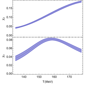
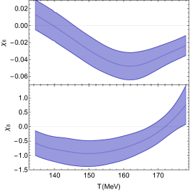
Figure 3: The HotQCD data for Taylor coefficients of the equation of state, Eq. (7), for $\mu_{Q}=\mu_{S}=0$ from Ref. Bollweg:2022rps . The bands denote the continuum extrapolation for $\chi_{2}$ and $\chi_{4}$ and spline extrapolation from the $N_{\tau}=8$ data for $\chi_{6}$ and $\chi_{8}$.

Given we have four terms in the Taylor expansion, the diagonal Padé resummation is a ratio of two quadratic polynomials in $\mu_{B}^{2}$. Analytical expressions for the poles and zeroes of Padé Bollweg:2022rps as well as conformal Padé can be obtained, however their functional forms do not play a central role in our analysis and to keep our discussion concise we will not include them here.

In order to take into account the statistical uncertainties, we have sampled an ensemble of coefficients from a Gaussian distribution. We used diagonal (2,2) Padé resummation which has a complex conjugate pair of poles. Since there are no other poles to form an accumulation point, we used these two poles values as estimators for the LY singularities, $|\mu_{LY}^{2}|e^{\pm i\theta}$. Repeating this for different temperatures we constructed the LY trajectory seen in Fig. 6. We also found that the zeroes did not follow any meaningful pattern. This is likely due to $N$ being relatively small.

With the conformal maps, there is one more step in extracting the singularity. As we mentioned in the previous section, the conformal maps explicitly depend on the location of the singularity. We first use the Padé estimate for the singularity in the conformal map and then follow the iterative procedure described in Section III to refine the estimate for $|\mu_{LY}^{2}|e^{\pm i\theta}$. The results of this procedure are shown in Figs. 4 and Fig. 5.

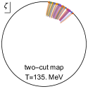
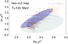
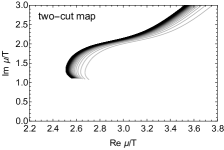
Figure 4: The iterative procedure of extracting the singularities via the two-cut conformal map. Each line represent the trajectory that corresponds to a set of Taylor coefficients sampled form a gaussian ensemble. The solid blue (green) disks denote the $1\sigma$ uncertainty region for two-cut and ordinary Padé resummations. Further description in text.

In Fig. 4 we show the trajectory of the iteration for different set of Taylor coefficients sampled from a gaussian ensemble. Each line with color represents the iteration obtained with fixed set of Taylor coefficients sampled from a gaussian ensemble, in the $\zeta$ (left) and $\mu_{B}$ (right) planes. The final estimate for each trajectory is denoted by a small solid disk. Each disk and the iteration curve are color coded. The pale blue disk in the center figure represent $1\sigma$ uncertainty region. For comparison, we also included the $1\sigma$ uncertainty region for the ordinary Padé resummation with the same temperature and ensemble of Taylor coefficients. The right figure shows the LY trajectory for a single, fixed set of Taylor coefficients. Different opacities denote different steps in the iteration, darker being later. Recall that the image of the true singularity of the equation of state in the $\zeta$ plane is along the unit disk (see Figs. 1 and 2). Remarkably the iteration indeed converges to the edge of the unit disk. In Fig. 5 we show the same trajectories for the uniformizing map. We used the same ensemble of Taylor coefficients for ordinary Padé as well as the two conformal maps.

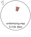
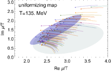
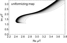
Figure 5: The iterative procedure of extracting the singularities via the uniformizing conformal map. Each line represent the trajectory that corresponds to a set of Taylor coefficients sampled form a gaussian ensemble. The solid blue (green) disks denote the $1\sigma$ uncertainty region for uniformizing and ordinary Padé resummations. Further description in text.

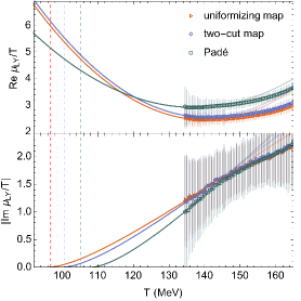
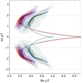
Figure 6: The Lee-Yang trajectory constructed via different resummations. The solid lines denote the fits for real and imaginary parts given in Eq. (21). The dashed vertical lines denote the extrapolation to $\mu_{c}^{2}$. Where the fit for the real part intersects the dashed lines leads to the extrapolation of $T_{c}$. The ellipses represent $1\sigma$ uncertainty stemming from the noise in the Taylor coefficients.

The LY trajectories constructed from different resummations are shown in Fig. 6. Each point for conformal Padé is obtained after 100 iterations as described above. The error bars represent the $1\sigma$ uncertainties inherited from the statistical uncertainties in the Taylor coefficients. Our next goal is to extract the location of the critical point from the LY trajectory. The critical chemical potential, $\mu_{c}$ is the point where ${\rm Im}\mu_{LY}$ vanishes. If there is a critical point, $\mu_{c}$ is clearly beyond the available data as ${\rm Im}\mu_{LY}>0$ for the temperature range in hand. At the same time the fact that ${\rm Im}\mu_{LY}$ is decreasing with decrasing temperature is suggestive that if there is a critical point, it lies at $T_{c}<135$ MeV. By extrapolating the trajectory to the point where ${\rm Im}\mu_{LY}=0$ we estimate $\mu_{c}$ and $T_{c}$. We using the following fits for the extrapolation:

$${\rm Re}\mu_{LY}(T) = a_{0}+a_{1}(T-T_{c})+a_{2}(T-T_{c})^{2}$$ (20)

$${\rm Im}\mu_{LY}(T) = a(T-T_{c})^{\beta\delta}$$ (21)

whose form is motivated by the scaling form given in Eq. (II). The results for the best-fits for different resummations are shown in Fig. 6 as solid lines. In these fits, we used the first 20 terms in the trajectory with $134.5\leq T\leq 144$. Finally from these fits we extrapolate the location of the critical point, as well as the non-universal mapping parameters, the slope of the crossover line at the critical point, $\alpha_{1}$, and $c_{2}$ as given in. Eq. (II). These results are listed in Table 1.

	$T_{c}$ (MeV)	$\mu_{c}$ (MeV)	crossover slope ($\alpha_{1}$)	$c_{2}$
uniformizing	97	579	$9.40^{\circ}$	2.22
two-cut	100	557	$8.69^{\circ}$	2.56
Padé	108	437	$4.55^{\circ}$	3.35

Table 1: The location of the critical point and the Ising model mapping parameters given in Eq. (II) extracted from Padé and conformal Padé.

Our final set of results concerns the Padé and conformal Padé resummations by using the Taylor coefficients of the susceptibility given in Eq. (19). A particularly interesting result we obtained from this resummation is the susceptibility as a function of chemical potential, shown in Fig. 7. The band denotes the $1\sigma$ uncertainty as before. Finally we show the singularities obtained this way in Fig. 8. For comparison, we also included the uniformizing map results for the singularities obtained from the expansion of pressure in the same figure (in purple).

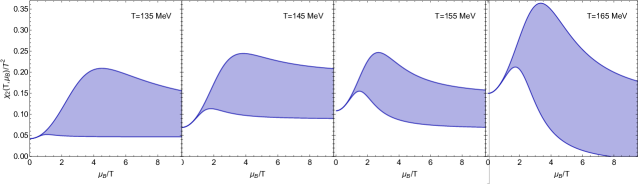
Figure 7: The susceptibility as a function of $\mu_{B}$ for four different temperatures calculated via the uniformizing conformal Padé from the Taylor coefficients of the susceptibility given in Eq. (19).

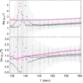
Figure 8: The poles of Padé and conformal Padé extracted from the Taylor coefficients of susceptibility compared with those extracted from the pressure.

Notice that using the coefficients of susceptibility reproduces qualitatively the expected behavior of $\chi$ as a function $\mu_{B}$, namely exhibiting a peak at some nonzero value of $\mu_{B}/T$, albeit with sizable statistical uncertainty. At the same time, the singularities extracted this way are less reliable compared to using the coefficients of pressure. We have found that the conformal Padé singularities in the $\zeta$ plane were much further away from the edge of the unit disk than those obtained from the coefficient of pressure. Furthermore the statistical errors are very large, especially for $T\lesssim 145$ MeV. This is ultimately because the, Padé and conformal Padé singularities depend rather sensitively on $\chi_{6}$ which changes sign around $140$ MeV, making the relative error quite large. Due to the difference in the functional dependence of the Padé singularities in the coefficients, this is not the case for the expansion of pressure. Therefore we conclude for the estimation of the location of singularities using coefficients of pressure is more reliable. However, using the coefficients of $\chi$ seem to reproduce the qualitatively expected form of the equation of state better. A more detailed analysis of this observation is left for future work.

V Summary and Discussion

The task of extracting the location of the Lee-Yang singularities from the presently available lattice QCD data is a challenging one. We only have access to four coefficients with sizable statistical uncertainties. In this paper, we utilized various conformal maps to improve the accuracy of the usual Padé resummation. By choosing appropriately designed conformal maps, we incorporated further analytical information regarding the equation of state, in addition to the Taylor coefficients; namely the closest singularities must be complex conjugate pair, i.e. the equation of state must be defined on a two-cut Riemann surface. We then conformally mapped this surface into the unit disk and extracted the Padé singularities there. Performing Padé resummation on a compact space gave a better handle in pinning down the location of the true singularity.

In order to take into account the statistical uncertainties in the Taylor coefficients we sampled them from a gaussian ensemble. The error due to the small number of Taylor coefficients, on the other hand, is harder to quantify. For large number of Taylor coefficients, there is a scaling relation between the magnitude of noise in the Taylor coefficients and the expansion order before (conformal) Padé resummation breaks down Costin:2022hgc . However it is an asymptotic result whose applicability to four terms is unclear.

In order to refine our estimation for the location of the singularity we built a novel iterative tool. Remarkably for both conformal maps, the iteration brought the images of the singularities extracted from conformal Padé closer to the edge of the unit disk where the real singularity lies, as seen in Figs. 4, 5. This observation increases our confidence in the results of conformal Padé. Note that, the uniformizing map is exponentially sensitive to the location of the singularity. Therefore it is not surprising that the poles in $\zeta$ plane for the uniformizing map are further away from the edge of the unit disk since we neither have enough number Taylor coefficients nor the precision to resolve singularity with exponential accuracy. It is also worth pointing out that the final results obtained from both conformal maps agree with each other and systematically differ from those from ordinary Padé. Furthermore the conformal Padé results are less sensitive to the statistical uncertainties compared to Padé which can be seen in Figs. 4, 5 and II. We think that for these reasons, conformal Padé results are more trustworthy than those of Padé.

Then, from the LY trajectory constructed via the resummations, we extrapolated the location of the critical point, as well as constrained values of the non-universal mapping parameters in its vicinity. These results are given in Table 1. This is the central result of our paper. Notice that we have used several significant figures in our extrapolation. This is not because we have such a precision in our computation, but to illustrate the quantitative differences between different resummations. The fact that they all lie in the same overall region is encouraging. Our results also agree with other results computed via similar Padé type resummations Clarke:2023noy , as well as other methods such as functional renormalization group Fu:2019hdw and truncated Dyson Schwinger equations Bernhardt:2021iql . Our estimate $\mu_{c}/T_{c}\approx 6$ is consistent with the constraints from the recent lattice QCD data which strongly disfavor the existence of a critical point for $\mu_{c}/T_{c}\lesssim 3$ Borsanyi:2020fev .

Of course, we had to rely on the best fits for our estimates for the critical point since the extrapolated $T_{c}$ is fairly lower than the minimum available temperature. Especially ${\rm Re}\mu_{LY}$, from which we extrapolate $T_{c}$, depends sensitively on the fit. Therefore, having access to lattice data for lower temperatures in the future would significantly improve the accuracy of the estimation of the location of the critical point.

Another important point we would like to discuss is that we assumed the equation of state obeys the scaling obtained from the universality class of the “$Z_{2}$ critical point” for part of the available temperature range for the LY trajectory in order to extrapolate the data to $\mu_{c}$ and $T_{c}$. In this scaling, the relevant axes mapped to the Ising parameters $h$ and $r$, are identified as $\mu_{B}$ and $T$. At the moment, it is unclear whether this scaling is valid at these temperatures. It is widely believed that around the pseudo-critical temperature, the closest singularity is associated with the “$O(4)$ critical point” that is located at $\mu_{B}=m_{u,d}=0$ which belongs to the $O(4)$ universality class. Therefore the LY trajectory should obey the “$O(4)$ scaling” which has a different form than the $Z_{2}$ scaling we used in Eq. (II). This is because the $O(4)$ scaling identifies one of relevant axes with the quark mass. Even though the agreement between the data and the form predicted by the $Z_{2}$ scaling seems suggestive that, at least for $T\in(130-145)$ MeV range, the $Z_{2}$ scaling is valid, this point requires further investigation. We shall address this issue in a forthcoming publication.

Finally, a related issue concerns the shape of the LY trajectory. In various models that exhibit similar critical phenomena to the conjectured QCD phase diagram, the LY trajectory can be exactly calculated. Among them are the Gross-Neveu model Basar:2021hdf , quark meson model Mukherjee:2021tyg and the Chiral Random Matrix model Stephanov:2006dn ; Basar:2021gyi where ${\rm Re}\mu_{LY}(T)$ and ${\rm Im}\mu_{LY}(T)$ are monotonically decreasing and increasing functions of $T$ respectively, for $T>T_{c}$. As seen in Fig. 6, the QCD data indicates that ${\rm Re}\mu_{LY}$ is not monotonically decreasing in $T$. For $T\gtrsim 145$ MeV, it is actually increasing. If this behavior is indeed representative of the physical LY trajectory and not an artifact of the resummations due to a combination of noise and small number of Taylor coefficients, it asks for further investigation. In fact, at higher temperatures, the shape of the LY trajectory is expected to be controlled by yet another singular point; the Roberge-Weiss singularity Roberge:1986mm and for some $T=T_{RW}$, the trajectory should pass through the point(s) ${\rm Re}\mu_{LY}(T_{RW})=0$, ${\rm Im}\mu_{LY}(T_{RW})=\pm\pi$. A recent estimate for the Roberge-Weiss temperature based on multi-point Padé approxmiants is $T_{RW}\approx 170$ MeV Schmidt:2022ogw . This means that, if the non-monotonic behavior is correct, then for some $T\in(160-170)$ MeV , ${\rm Re}\mu_{LY}(T)$ has to peak and then go down to zero. At the same time, because $\chi_{8}$ crosses zero around $T\approx 170$ MeV, the Padé singularities are too noisy around these temperatures to lead to any meaningful estimation of $\mu_{LY}$. Note that the Roberge-Weiss point is related to confinement/deconfinement transition and therefore is not present in any of the aforementioned models. We leave this discussion to be addressed in a future publication as well.

VI Acknowledgments

We thank M. Stephanov and G. Dunne for fruitful discussions. The author is supported by the National Science Foundation CAREER Award PHY-2143149.

References

- (1) Y. Aoki, G. Endrodi, Z. Fodor, S. D. Katz, and K. K. Szabo, “The Order of the quantum chromodynamics transition predicted by the standard model of particle physics,” Nature 443 (2006) 675–678, arXiv:hep-lat/0611014.
- (2) O. Philipsen, “Lattice qcd at finite temperature and density,” The European Physical Journal Special Topics 152 no. 1, (2007) 29–60. https://doi.org/10.1140/epjst/e2007-00376-3.
- (3) P. de Forcrand, “Simulating QCD at finite density,” PoS LAT2009 (2009) 010, arXiv:1005.0539 [hep-lat].
- (4) H.-T. Ding, F. Karsch, and S. Mukherjee, “Thermodynamics of strong-interaction matter from Lattice QCD,” Int. J. Mod. Phys. E 24 no. 10, (2015) 1530007, arXiv:1504.05274 [hep-lat].
- (5) A. Bzdak, S. Esumi, V. Koch, J. Liao, M. Stephanov, and N. Xu, “Mapping the Phases of Quantum Chromodynamics with Beam Energy Scan,” Phys. Rept. 853 (2020) 1–87, arXiv:1906.00936 [nucl-th].
- (6) D. Almaalol et al., “QCD Phase Structure and Interactions at High Baryon Density: Continuation of BES Physics Program with CBM at FAIR,” arXiv:2209.05009 [nucl-ex].
- (7) C. R. Allton, S. Ejiri, S. J. Hands, O. Kaczmarek, F. Karsch, E. Laermann, C. Schmidt, and L. Scorzato, “The QCD thermal phase transition in the presence of a small chemical potential,” Phys. Rev. D 66 (2002) 074507, arXiv:hep-lat/0204010.
- (8) P. de Forcrand and O. Philipsen, “The QCD phase diagram for small densities from imaginary chemical potential,” Nucl. Phys. B 642 (2002) 290–306, arXiv:hep-lat/0205016.
- (9) M. D’Elia and M.-P. Lombardo, “Finite density QCD via imaginary chemical potential,” Phys. Rev. D 67 (2003) 014505, arXiv:hep-lat/0209146.
- (10) R. Bellwied, S. Borsanyi, Z. Fodor, J. Günther, S. D. Katz, C. Ratti, and K. K. Szabo, “The QCD phase diagram from analytic continuation,” Phys. Lett. B 751 (2015) 559–564, arXiv:1507.07510 [hep-lat].
- (11) C. Ratti, “Lattice QCD and heavy ion collisions: a review of recent progress,” Rept. Prog. Phys. 81 no. 8, (2018) 084301, arXiv:1804.07810 [hep-lat].
- (12) S. Borsányi, Z. Fodor, J. N. Guenther, R. Kara, S. D. Katz, P. Parotto, A. Pásztor, C. Ratti, and K. K. Szabó, “Lattice QCD equation of state at finite chemical potential from an alternative expansion scheme,” arXiv:2102.06660 [hep-lat].
- (13) HotQCD Collaboration, D. Bollweg, J. Goswami, O. Kaczmarek, F. Karsch, S. Mukherjee, P. Petreczky, C. Schmidt, and P. Scior, “Taylor expansions and Padé approximants for cumulants of conserved charge fluctuations at nonvanishing chemical potentials,” Phys. Rev. D 105 no. 7, (2022) 074511, arXiv:2202.09184 [hep-lat].
- (14) HotQCD Collaboration, D. Bollweg, D. A. Clarke, J. Goswami, O. Kaczmarek, F. Karsch, S. Mukherjee, P. Petreczky, C. Schmidt, and S. Sharma, “Equation of state and speed of sound of (2+1)-flavor QCD in strangeness-neutral matter at nonvanishing net baryon-number density,” Phys. Rev. D 108 no. 1, (2023) 014510, arXiv:2212.09043 [hep-lat].
- (15) S. Borsanyi, Z. Fodor, J. N. Guenther, R. Kara, S. D. Katz, P. Parotto, A. Pasztor, C. Ratti, and K. K. Szabo, “QCD Crossover at Finite Chemical Potential from Lattice Simulations,” Phys. Rev. Lett. 125 no. 5, (2020) 052001, arXiv:2002.02821 [hep-lat].
- (16) M. E. Fisher, “Critical point phenomena - the role of series expansions,” Rocky Mountain Journal of Mathematics 4 no. 2, (1974) 181.
- (17) M. Halasz, A. Jackson, and J. Verbaarschot, “Yang-lee zeros of a random matrix model for qcd at finite density,” Physics Letters B 395 no. 3-4, (Mar, 1997) 293–297. http://dx.doi.org/10.1016/S0370-2693(97)00015-4.
- (18) S. Ejiri, “Lee-Yang zero analysis for the study of QCD phase structure,” Phys. Rev. D 73 (2006) 054502, arXiv:hep-lat/0506023.
- (19) M. A. Stephanov, “QCD critical point and complex chemical potential singularities,” Phys. Rev. D 73 (2006) 094508, arXiv:hep-lat/0603014.
- (20) S. Mukherjee and V. Skokov, “Universality driven analytic structure of the QCD crossover: radius of convergence in the baryon chemical potential,” Phys. Rev. D 103 no. 7, (2021) L071501, arXiv:1909.04639 [hep-ph].
- (21) A. Connelly, G. Johnson, S. Mukherjee, and V. Skokov, “Universality driven analytic structure of QCD crossover: radius of convergence and QCD critical point,” Nucl. Phys. A 1005 (2021) 121834, arXiv:2004.05095 [hep-ph].
- (22) G. Basar, “Universality, Lee-Yang Singularities, and Series Expansions,” Phys. Rev. Lett. 127 no. 17, (2021) 171603, arXiv:2105.08080 [hep-th].
- (23) G. Basar, G. V. Dunne, and Z. Yin, “Uniformizing Lee-Yang singularities,” Phys. Rev. D 105 no. 10, (2022) 105002, arXiv:2112.14269 [hep-th].
- (24) P. Dimopoulos, L. Dini, F. Di Renzo, J. Goswami, G. Nicotra, C. Schmidt, S. Singh, K. Zambello, and F. Ziesché, “Contribution to understanding the phase structure of strong interaction matter: Lee-Yang edge singularities from lattice QCD,” Phys. Rev. D 105 no. 3, (2022) 034513, arXiv:2110.15933 [hep-lat].
- (25) G. Nicotra, P. Dimopoulos, L. Dini, F. Di Renzo, J. Goswami, C. Schmidt, S. Singh, K. Zambello, and F. Ziesche, “Lee-Yang edge singularities in 2+1 flavor QCD with imaginary chemical potential.,” PoS LATTICE2021 (2022) 260, arXiv:2111.05630 [hep-lat].
- (26) Bielefeld-Parma Collaboration, S. Singh, P. Dimopoulos, L. Dini, F. Di Renzo, J. Goswami, G. Nicotra, C. Schmidt, K. Zambello, and F. Ziesche, “Lee-yang edge singularities in lattice qcd : A systematic study of singularities in the complex mub plane using rational approximations.,” PoS LATTICE2021 (2022) 544, arXiv:2111.06241 [hep-lat].
- (27) C. Schmidt, D. A. Clarke, G. Nicotra, F. Di Renzo, P. Dimopoulos, S. Singh, J. Goswami, and K. Zambello, “Detecting Critical Points from the Lee–Yang Edge Singularities in Lattice QCD,” Acta Phys. Polon. Supp. 16 no. 1, (2023) 1–A52, arXiv:2209.04345 [hep-lat].
- (28) D. A. Clarke, K. Zambello, P. Dimopoulos, F. Di Renzo, J. Goswami, G. Nicotra, C. Schmidt, and S. Singh, “Determination of Lee-Yang edge singularities in QCD by rational approximations,” PoS LATTICE2022 (2023) 164, arXiv:2301.03952 [hep-lat].
- (29) P. Parotto, M. Bluhm, D. Mroczek, M. Nahrgang, J. Noronha-Hostler, K. Rajagopal, C. Ratti, T. Schäfer, and M. Stephanov, “QCD equation of state matched to lattice data and exhibiting a critical point singularity,” Phys. Rev. C 101 no. 3, (2020) 034901, arXiv:1805.05249 [hep-ph].
- (30) X. An et al., “The BEST framework for the search for the QCD critical point and the chiral magnetic effect,” Nucl. Phys. A 1017 (2022) 122343, arXiv:2108.13867 [nucl-th].
- (31) X. An, D. Mesterházy, and M. A. Stephanov, “Functional renormalization group approach to the Yang-Lee edge singularity,” JHEP 07 (2016) 041, arXiv:1605.06039 [hep-th].
- (32) X. An, D. Mesterházy, and M. A. Stephanov, “On spinodal points and Lee-Yang edge singularities,” J. Stat. Mech. 1803 no. 3, (2018) 033207, arXiv:1707.06447 [hep-th].
- (33) P. Fonseca and A. Zamolodchikov, “Ising field theory in a magnetic field: Analytic properties of the free energy,” arXiv:hep-th/0112167.
- (34) C.-N. Yang and T. D. Lee, “Statistical theory of equations of state and phase transitions. 1. Theory of condensation,” Phys. Rev. 87 (1952) 404–409.
- (35) T. D. Lee and C.-N. Yang, “Statistical theory of equations of state and phase transitions. 2. Lattice gas and Ising model,” Phys. Rev. 87 (1952) 410–419.
- (36) J. Zinn-Justin, “Quantum field theory and critical phenomena,” Int. Ser. Monogr. Phys. 113 (2002) 1–1054.
- (37) S. El-Showk, M. F. Paulos, D. Poland, S. Rychkov, D. Simmons-Duffin, and A. Vichi, “Solving the 3d ising model with the conformal bootstrap,” Phys. Rev. D 86 (Jul, 2012) 025022. https://link.aps.org/doi/10.1103/PhysRevD.86.025022.
- (38) F. Rennecke and V. V. Skokov, “Universal location of Yang–Lee edge singularity for a one-component field theory in 1d4,” Annals Phys. 444 (2022) 169010, arXiv:2203.16651 [hep-ph].
- (39) A. Connelly, G. Johnson, F. Rennecke, and V. Skokov, “Universal Location of the Yang-Lee Edge Singularity in Theories,” Phys. Rev. Lett. 125 no. 19, (2020) 191602, arXiv:2006.12541 [cond-mat.stat-mech].
- (40) G. Johnson, F. Rennecke, and V. V. Skokov, “Universal location of Yang-Lee edge singularity in classic O(N) universality classes,” Phys. Rev. D 107 no. 11, (2023) 116013, arXiv:2211.00710 [hep-ph].
- (41) F. Karsch, C. Schmidt, and S. Singh, “Lee-Yang and Langer edge singularities from analytic continuation of scaling functions,” arXiv:2311.13530 [hep-lat].
- (42) M. E. Fisher, “Yang-Lee Edge Singularity and phi**3 Field Theory,” Phys. Rev. Lett. 40 (1978) 1610–1613.
- (43) M. S. Pradeep and M. Stephanov, “Universality of the critical point mapping between Ising model and QCD at small quark mass,” Phys. Rev. D 100 no. 5, (2019) 056003, arXiv:1905.13247 [hep-ph].
- (44) A. Bazavov et al., “The QCD Equation of State to from Lattice QCD,” Phys. Rev. D 95 no. 5, (2017) 054504, arXiv:1701.04325 [hep-lat].
- (45) M. Giordano, K. Kapas, S. Katz, D. Nogradi, and A. Pasztor, “Towards a reliable lower bound on the location of the critical endpoint,” Nuclear Physics A 1005 (2021) 121986. https://www.sciencedirect.com/science/article/pii/S0375947420302967. The 28th International Conference on Ultra-relativistic Nucleus-Nucleus Collisions: Quark Matter 2019.
- (46) H. Stahl, “The convergence of padé approximants to functions with branch points,” Journal of Approximation Theory 91 no. 2, (1997) 139–204. https://www.sciencedirect.com/science/article/pii/S0021904597931415.
- (47) E. Saff Surveys in Approximation Theory 5 (2010) 165–200.
- (48) O. Costin and G. V. Dunne, “Uniformization and Constructive Analytic Continuation of Taylor Series,” arXiv:2009.01962 [math.CV].
- (49) R. Guida and J. Zinn-Justin, “Critical exponents of the N vector model,” J. Phys. A 31 (1998) 8103–8121, arXiv:cond-mat/9803240.
- (50) R. Rossi, T. Ohgoe, K. Van Houcke, and F. Werner, “Resummation of diagrammatic series with zero convergence radius for strongly correlated fermions,” Phys. Rev. Lett. 121 (Sep, 2018) 130405. https://link.aps.org/doi/10.1103/PhysRevLett.121.130405.
- (51) M. Serone, G. Spada, and G. Villadoro, “ theory — Part II. the broken phase beyond NNNN(NNNN)LO,” JHEP 05 (2019) 047, arXiv:1901.05023 [hep-th].
- (52) O. Costin and G. V. Dunne, “Physical Resurgent Extrapolation,” Phys. Lett. B 808 (2020) 135627, arXiv:2003.07451 [hep-th].
- (53) O. Costin and G. V. Dunne, “Conformal and uniformizing maps in Borel analysis,” Eur. Phys. J. ST 230 no. 12-13, (2021) 2679–2690, arXiv:2108.01145 [hep-th].
- (54) O. Costin, G. V. Dunne, and M. Meynig, “Noise effects on Padé approximants and conformal maps ∗,” J. Phys. A 55 no. 46, (2022) 464007, arXiv:2208.02410 [math-ph].
- (55) W.-j. Fu, J. M. Pawlowski, and F. Rennecke, “QCD phase structure at finite temperature and density,” Phys. Rev. D 101 no. 5, (2020) 054032, arXiv:1909.02991 [hep-ph].
- (56) J. Bernhardt, C. S. Fischer, P. Isserstedt, and B.-J. Schaefer, “Critical endpoint of QCD in a finite volume,” Phys. Rev. D 104 no. 7, (2021) 074035, arXiv:2107.05504 [hep-ph].
- (57) S. Mukherjee, F. Rennecke, and V. V. Skokov, “Analytical structure of the equation of state at finite density: Resummation versus expansion in a low energy model,” Phys. Rev. D 105 no. 1, (2022) 014026, arXiv:2110.02241 [hep-ph].
- (58) A. Roberge and N. Weiss, “Gauge Theories With Imaginary Chemical Potential and the Phases of QCD,” Nucl. Phys. B 275 (1986) 734–745.