Perseus: Removing Energy Bloat from Large Model Training

Abstract

Training large AI models on numerous GPUs consumes a massive amount of energy. We observe that not all energy consumed during training directly contributes to end-to-end training throughput, and a significant portion can be removed without slowing down training, which we call energy bloat.

In this work, we identify two independent sources of energy bloat in large model training, intrinsic and extrinsic, and propose Perseus, a unified optimization framework that mitigates both. Perseus obtains the “iteration time–energy” Pareto frontier of any large model training job using an efficient iterative graph cut-based algorithm and schedules energy consumption of its forward and backward computations across time to remove intrinsic and extrinsic energy bloat. Evaluation on large models like GPT-3 and Bloom shows that Perseus reduces energy consumption of large model training by up to 30%, enabling savings otherwise unobtainable before.

1 Introduction

As deep neural networks (DNNs) continue to grow in model and dataset size [29, 25], the energy consumption of large model training is increasing as well. For instance, training GPT-3 [11] reportedly consumed 1,287 megawatt-hour (MWh) in 2021 [48]. The recent surge in the development of generative AI (GenAI) and large language models (LLMs) shows no signs of deceleration in AI energy demands.

Optimizing the energy consumption of large model training is, therefore, crucial to minimizing the operational costs associated with AI, with additional benefits. For example, low-carbon electricity, which is preferred especially in the context of sustainability commitments [1, 4, 6, 7], is still very much a scarce and contended resource [50]. Reducing energy consumption allows more workloads to fit within the limited supply of low-carbon electricity [10]. Furthermore, reducing energy consumption without slowdown reduces power draw, either allowing more aggressive datacenter power oversubscription or conversely reducing power throttling for existing workloads [35, 54, 46].

Despite many recent works on increasing the throughput of large model training [26, 41, 19, 43, 73, 34, 27], reining in the growing energy consumption remains an open challenge [55, 48]. In this paper, we aim to identify and remove energy bloat – the portion of energy consumption that can be removed without throughput loss – in large model training. We identify two independent sources of energy bloat: intrinsic and extrinsic, and propose a single optimization framework that minimizes both.

Intrinsic energy bloat comes from computation imbalance when a large model is distributed across multiple GPUs with pipeline parallelism (§2.2). Balancing the amount of computation in each pipeline stage is an important problem for distributed execution planning [41, 19, 23, 73], but perfectly balancing every stage is not always possible because layers in a DNN are coarse-grained tensor operations with varying amounts of computation. When all stages do not have the same computation intensity, those not on the critical path of computation run needlessly fast – i.e., they consume energy that does not contribute to the overall training throughput. Such intrinsic energy bloat opens up the opportunity to precisely slow down each non-critical computation in the pipeline such that the length of the critical path does not change.

Extrinsic energy bloat, in contrast, arises when multiple pipelines run in parallel in a synchronous fashion to scale out training to massive datasets, and one or more pipelines run slower than the others (§2.3). Root causes behind such slowdowns are varied, including power/thermal throttling [75, 47, 35, 54, 46], I/O bottlenecks in the storage/network [39, 71], hardware/software failures [61, 27], etc., and the likelihood of their presence increases with the scale and duration of training [22, 28, 64]. All pipelines running faster than the straggler pipeline are needlessly fast and wasting energy that does not affect the overall training throughput. Extrinsic energy bloat allows us to slow down entire pipelines (while still keeping their intrinsic energy bloat low) without delaying gradient synchronization.

In this work, we propose Perseus that relies on a unified optimization framework to remove both intrinsic and extrinsic energy bloat during large model training (§3). At its core, Perseus efficiently pre-characterizes the entire “iteration time–energy” Pareto frontier, which enables it to minimize intrinsic energy bloat under normal operating conditions and to mitigate extrinsic energy bloat arising from straggler pipelines. Existing works fall short on both fronts. EnvPipe [13] is limited only to intrinsic bloat reduction with a point solution that leads to suboptimal energy reduction. Zeus [68], in contrast, ignores intrinsic bloat altogether as it only considers single-GPU training, which also leads it to identify suboptimal “iteration time–energy” frontiers at best.

We prove that optimally solving our optimization problem is in fact NP-hard and propose an efficient algorithm that provides an exact solution for a relaxed problem (§4). At its core, our solution represents an iteration of large model training as a directed acyclic graph (DAG). Each node in the DAG represents either a forward or backward computation in a particular stage, and nodes are connected with edges that represent computation dependencies. Importantly, each node is annotated with its planned execution time and energy consumption, which we call the energy schedule. Perseus’s optimization algorithm starts from the energy schedule that consumes the least possible amount of energy, and iteratively speeds up the execution time of the schedule while incurring the least possible energy increase, until no more speed up is possible. This generates all energy schedules on the “iteration time–energy” Pareto frontier. Minimizing intrinsic and/or extrinsic energy bloat is then as simple as choosing the appropriate energy schedule from the Pareto frontier.

While solving the optimization problem depends on accurate fine-grained computation energy profiling, modern GPUs provide energy consumption information only in coarse-grained time intervals. Perseus introduces an online profiling technique that can accurately profile the energy consumption of fine-grained computations with low overhead (§5).

Evaluation on a variety of large models including GPT-3 [11], BERT [15], T5 [51], Bloom [66] and a scaled-up version of Wide-ResNet [69] shows that Perseus is able to reduce per-iteration energy consumption by up to 30% with negligible or no slowdown (§6).

Overall, we make the following contributions in this paper:

• We identify intrinsic and extrinsic energy bloat in large model training, fundamentally caused by computation time imbalance at different levels.

• We propose Perseus, an open-source unified optimization framework that aims to remove both types of energy bloat using an efficient graph cut-based algorithm.

• We evaluate Perseus on a diverse set of large model workloads and show that it significantly reduces energy bloat.

2 Motivation

First, we provide necessary background regarding large model training (§2.1). Then, we introduce intrinsic (§2.2) and extrinsic (§2.3) energy bloat present in large model training.

2.1 Large Model Training

The rapid increase in DNN model size in recent years made data, tensor, and pipeline parallelism [26, 41, 43, 19, 73, 34] essential ingredients for large model training. Especially, pipeline parallelism partitions a large model into multiple stages and assigns each stage to different GPUs. The training batch is split into multiple microbatches, and their forward and backward computations are pipelined through those stages. Then, in order to scale out to more GPUs, such pipelines are replicated multiple times to perform data parallel training, where each pipeline computes a subset of the training batch and synchronizes gradients with one other at the end of each iteration. Due to the synchronization barrier in the end, the next iteration can only begin when all pipelines have finished.

2.2 Intrinsic Energy Bloat

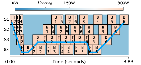
(a)

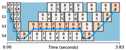
(b)

Figure 1: One training iteration of GPT-3 1.3B with 4 pipeline stages (partitioned with minimum imbalance ratio) and 6 microbatches on NVIDIA A100 GPUs drawn to scale. For example, F5 and B5 in the S2 row denote Forward and Backward for the fifth microbatch on Stage 2. The critical path of computation is traced with a blue line. Colors are average power consumption. The blue background indicates that GPUs consume power when blocking on communication.

Model	Size	Imbalance Ratio
		4 stages	8 stages
GPT-3 [11]	3B	1.13	1.25
	7B	1.11	1.23
	13B	1.08	1.17
	175B	1.02	1.03
Bloom [66]	3B	1.13	1.25
	7B	1.13	1.25
	176B	1.05	1.10
BERT [15]	0.1B	1.33	2.00
	0.3B	1.17	1.33
T5 [51]	0.2B	1.19	1.50
	0.7B	1.05	1.11
	2.9B	1.06	1.16
Wide-ResNet50 [69]	0.8B	1.23	1.46
Wide-ResNet101 [69]	1.5B	1.09	1.25

Table 1: Imbalance ratio between the longest and the shortest stages for various models on NVIDIA A100 GPUs. 1.00 would mean perfect balance.

We profile GPT-3 1.3B on NVIDIA A100 GPUs and visualize the timeline of one training iteration in Figure 1(a). In addition to the familiar bubbles found in any pipeline schedule [41], we observe gaps in between forward and backward computations, where the GPU is simply blocking on communication with an adjacent stage. Such gaps exist because the computation time of each pipeline stage is not perfectly balanced. Partitioning stages in a balanced manner is an important problem in distributed execution planning [26, 41, 19, 73], but perfect balancing is difficult because DNNs are essentially a sequence of coarse-grained tensor operations with varying size.

To understand the amount of possible pipeline stage imbalance, we exhaustively enumerated all possible pipeline partitions to find the one with the smallest imbalance ratio, defined as the ratio of the longest stage forward computation latency to the shortest. Table 1 lists the minimum imbalance ratio for various models, which shows that perfect balance is difficult to achieve. Appendix A explains the partitioning details of each model and where imbalance comes from.

Given some amount of stage imbalance, as we have seen in Figure 1(a), not all forward and backward computations are on the critical path of computation. This means that non-critical computations running at their maximum speed is not contributing to faster iteration time, and thus simply wasting energy. We call this intrinsic energy bloat, which can be reduced by precisely slowing down each non-critical computation so that they do not affect the critical path (Figure 1(b)). Although seemingly simple, we prove that this problem is NP-hard by reduction from the 0/1 Knapsack problem (Appendix B). Visualizations for other models are in Appendix C.

2.3 Extrinsic Energy Bloat

During large model training, numerous replicas of the same pipeline run in a data parallel fashion in order to train on more data with more GPUs, and every pipeline must synchronize gradients at the end of each iteration before moving on to the next. When one pipeline runs slower, all other pipelines must wait until the straggler pipeline finishes. Figure 2(a) illustrates this situation. Since the straggler pipeline determines end-to-end iteration time, all other pipelines running at their fastest possible iteration time are wasteful. We call this extrinsic energy bloat, because unlike intrinsic energy bloat, the cause of energy bloat is extrinsic to the pipeline.

Perseus finds the energy-optimal iteration time for the non-straggler pipeline, again by precisely slowing down computations in the pipeline (Figure 2(b)). However, unlike other problem settings that do not consider energy consumption, we show in Section 3.1 that fully utilizing all the slack time created by the straggler may not be energy-optimal! Perseus can automatically make such decisions and implements the energy-optimal slowdown.

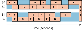
(a)

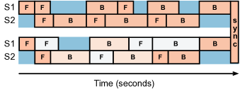
(b)

Figure 2: Toy example illustrating one straggler pipeline running together with a non-straggler pipeline using data parallelism. The non-straggler wastes energy by running as fast as possible. Perseus can precisely slow down non-straggler pipelines to reduce such extrinsic energy bloat.

Stragglers arise from numerous sources, with many introducing sizable energy bloat according to recent reports. Thermal or power throttling in a datacenter may lower the GPU’s frequency to prevent hardware or the power supply unit from being damaged, resulting in 10–50% slowdown [75, 47, 35, 54, 46]. I/O bottlenecks in the storage or network, especially during data loading for image, video, or recommendation models, can be longer than GPU computation by up to $4\times$ [39, 71], thereby acting like a persistent (virtual) straggler pipeline. Recent failure-resilient large model training frameworks [61, 27] deploy heterogeneous pipelines with different number of stages or amount of compute after failures, introducing non-uniform iteration times across pipelines until recovery. As the scale of large model training jobs increase, the probability of the job encountering one or more causes of stragglers increases [22, 28, 64].

Stragglers due to events like thermal/power throttling, consistent I/O bottlenecks, and fault-tolerant planning can persist across many iterations [46, 39, 27]. A training system can identify such stragglers and calculate the extent of slowdown by comparing iteration times across data-parallel pipelines. In this work, we assume that such knowledge is available and focus on how to plan time and energy consumption across time and allow quick adaptation given such information.

3 Perseus Overview

Perseus is an energy optimization system for large model training. In this section, we present our unified optimization framework that aims to remove both types of energy bloat (§3.1) and walk through the workflow of Perseus (§3.2).

3.1 Optimization Approach

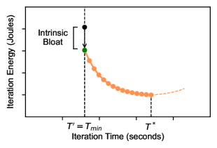
(a)

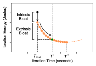
(b)

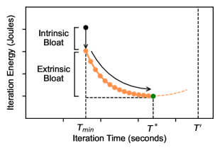
(c)

Figure 3: Three cases of where the straggler pipeline’s iteration time $T^{\prime}$ can be. The first case is when there are no stragglers. $T_{\min}$ and $T^{*}$ are the shortest and longest iteration time on the “iteration time–energy” Pareto frontier. The black dot is the default mode of execution where all computations run at the maximum speed. The green dot is the energy-optimal iteration time of the non-straggler pipeline.

Intuitively, slowing down computations selectively in a training pipeline without affecting its critical path will keep the same iteration time while reducing its energy consumption (§2.2). Furthermore, when stragglers emerge, slowing down computations in a non-straggler pipeline without making it a straggler itself will reduce energy consumption even more (§2.3). We formalize these two intuitions into a unified optimization framework and derive a universal prescription for a non-straggler pipeline’s energy-optimal iteration time.

By controlling the execution speed of individual computations in the pipeline, our goal is to minimize the energy consumption of a pipeline, and we can safely slow down a pipeline’s iteration time until the straggler’s iteration time $T^{\prime}$:

$$\min_{F} \quad\textrm{Energy}(F)$$ (1)

s.t. $$\quad\textrm{Time}(F)\leq T^{\prime}$$

where $F$ is the set of GPU frequencies to run each forward and backward computation in the pipeline, and $\textrm{Time}(F)$ and $\textrm{Energy}(F)$ are the iteration time and energy consumption of the pipeline when executed with $F$, respectively. Changing $F$ will lead to different values of $\textrm{Time}(F)$ and $\textrm{Energy}(F)$ on the “iteration time–energy” 2D plane. However, we are only interested in ($\textrm{Time}(F)$, $\textrm{Energy}(F)$) points that are on the “iteration time–energy” Pareto frontier, a monotonically decreasing tradeoff curve.

Figure 3 depicts the three cases where the straggler’s iteration time $T^{\prime}$ can possibly be w.r.t. the “iteration time–energy” Pareto frontier. $T_{min}$ is the shortest iteration time on the frontier, which coincides with the iteration time of running every computation at the maximum speed, and $T^{*}$ is the iteration time with minimum energy consumption. Together, $T_{\min}$ and $T^{*}$ bookend the Pareto frontier.

1. When there are no stragglers (Figure 3(a)), we simply operate on the point on the Pareto frontier with the same iteration time, which reduces intrinsic energy bloat.

2. When a moderately slow straggler is detected (Figure 3(b)), we additionally reduce extrinsic energy bloat by slowing down non-straggler pipelines until $T^{\prime}$, using up all the slack time created by the straggler.

3. Finally, when the straggler’s iteration time goes beyond the minimum-energy point $T^{*}$ on the frontier (Figure 3(c)), we stop at $T^{*}$ instead of $T^{\prime}$. This is because slowing down beyond $T^{*}$ will instead increase energy.

The three cases can be merged into one universal prescription for the pipeline’s energy-optimal iteration time:

$$T_{\textrm{opt}}=\min(T^{*},T^{\prime}).$$ (2)

Therefore, if we pre-characterize the entire “iteration time–energy” Pareto frontier, we know the solution of Equation 1 for any feasible value of $T^{\prime}$. Then our system will be able to react quickly to emerging stragglers by simply looking up the set of frequencies $F_{\textrm{opt}}$ that leads to iteration time $T_{\textrm{opt}}$. We present our algorithm to efficiently characterize the entire “iteration time–energy” Pareto frontier in Section 4.

3.2 Perseus Architecture

Energy Schedule.

Perseus represents each iteration of the training pipeline as a static directed acyclic graph (DAG), where nodes are forward and backward computations and edges are dependencies in between computations. Each node on the computation DAG is annotated with its planned time and energy consumption, which we call the energy schedule. Perseus realizes an energy schedule by executing each computation with a specific GPU frequency.

System Components.

Figure 4 shows the high-level architecture of Perseus. Perseus is split into a framework-independent server and a framework-integrated client. The server runs our time–energy optimization algorithm, produces all energy schedules on the “iteration time–energy” Pareto frontier, and caches them in a table for fast lookup. The client profiles computations of the pipelines online during training, and realizes the energy schedule by changing the GPU’s frequency during runtime.

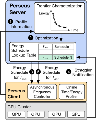
Figure 4: Perseus architecture and workflow.

Training Lifecycle Using Perseus.

In Perseus, a training job is specified by its computation DAG. When the job begins execution, the Perseus client invokes its Online Time/Energy Profiler (§5) to measure the time and energy consumption of each forward and backward computation in each stage while training is running, and sends the profile to the server.

As training proceeds, the server asynchronously characterizes the “iteration time–energy” Pareto frontier of the training job (§4), after which the Pareto-optimal energy schedule corresponding to the shortest possible iteration time $T_{\min}$ is deployed to the client. Energy schedules are realized by the client’s Asynchronous Frequency Controller, integrated into the training framework’s pipeline execution engine (§5). Pareto-optimal energy schedules are saved in a lookup table format index by $T^{\prime}$.

During training, the hardware infrastructure (e.g., data center rack power manager) notifies the Perseus server of a straggler pipeline and how much slowdown it will experience. The Perseus server can quickly react to this by looking up the Pareto-optimal energy schedule corresponding to that straggler iteration time, and deploying it to the clients.

4 Algorithm Design

In this section, we describe our algorithm to obtain the “iteration time–energy” Pareto frontier for a training pipeline in detail. We start by formulating the problem (§4.1). Then, we provide an overview of our algorithm (§4.2) and describe the core subroutine in our algorithm (§4.3). Finally, we extend our algorithm to support tensor parallelism, single-choice operations, and diverse pipeline schedules (§4.4).

4.1 Problem Formulation

Expression for Energy Consumption.

The energy consumption of a pipeline is not only from computation; it is the sum of three parts: (1) Computation; (2) Blocking on communication between computations; and (3) Blocking on communication until the straggler pipeline finishes. Formally,

$$\sum_{i}{e_{i}(f_{i})}+P_{\textrm{blocking}}(N\cdot T-\sum_{i}{t_{i}(f_{i})})+P_{\textrm{blocking}}\cdot N\cdot(T^{\prime}-T)$$ (3)

$$=\underset{\leavevmode\hbox to8.53pt{\vbox to8.53pt{\text{[drawing]}}}}{\underline{\sum_{i}{\left(e_{i}(f_{i})-P_{\textrm{blocking}}\cdot t_{i}(f_{i})\right)}}}+\underset{\leavevmode\hbox to8.53pt{\vbox to8.53pt{\text{[drawing]}}}}{\underline{\vphantom{\sum_{i}}P_{\textrm{blocking}}\cdot N\cdot T^{\prime}}}$$

where $P_{\textrm{blocking}}$ is the power consumption of the GPU when it is blocking on communication, $N$ is the number of pipeline stages, and $t_{i}(f_{i})$ and $e_{i}(f_{i})$ are the time and energy consumption of computation $i$ with frequency $f_{i}$, respectively.

Equation 3 shows that the “iteration time–energy” Pareto frontier of a pipeline depends on the straggler’s iteration time $T^{\prime}$ in . Specifically, the Pareto frontier for any $T^{\prime}$ is the Pareto frontier of $\textrm{Time}(F)$ vs. shifted upwards by . Here, does not depend on $T^{\prime}$. Therefore, if we characterize the Pareto frontier of $\textrm{Time}(F)$ vs. , that frontier can be used to find $T_{\textrm{opt}}$ and $F_{\textrm{opt}}$ for any value of $T^{\prime}$ as shifting the frontier upwards does not affect iteration time nor the frequency assignments that lead to each iteration time. Thus, we define

$$\textrm{Energy}(F)=\sum_{i}{\left(e_{i}(f_{i})-P_{\textrm{blocking}}\cdot t_{i}(f_{i})\right)}$$ (4)

and characterize the Pareto frontier of $\textrm{Time}(F)$ vs. $\textrm{Energy}(F)$.

Finding the Pareto Frontier.

Finding one point on the “iteration time–energy” Pareto frontier with iteration time $T^{\prime}$ is equivalent to solving the following optimization problem:

$$\min_{F} \quad\textrm{Energy}(F)$$ (5)

s.t. $$\quad\textrm{Time}(F)\leq T^{\prime}$$

We call this problem Pipeline Energy Minimization (PEM).

Theorem 1.

Pipeline Energy Minimization is NP-hard.

Proof.

Reduction from 0/1 Knapsack. Details in Appendix B. ∎

The complete Pareto frontier can be obtained by solving PEM for all $T^{\prime}\in[T_{\min},T^{*}]$, which is clearly intractable. Therefore, we seek an appropriate relaxation of the problem.

One of the reasons PEM is NP-hard is because it is a discrete optimization problem where the possible choices of computation time and energy are discrete, which is in turn because the possible choices of GPU frequencies are discrete. However, if choices were continuous, the problem is exactly and efficiently solvable [57]. This is akin to integer linear programs becoming tractable when relaxed to linear programs.

We fit the exponential function ($a\cdot e^{bt}+c$) to Pareto-optimal computation time and energy measurements to make the choices continuous. We choose the exponential function due to its inherent flexibility and natural fit to data. We show in Section 6 that this relaxation produces high-quality approximate solutions that lead to actual savings. After relaxation, the problem’s optimization variables are the time and energy consumption planned for each computation in the pipeline, or the energy schedule.

4.2 Algorithm Overview

Iteratively Discovering the Pareto Frontier.

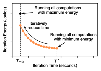
Figure 5: Starting from the Pareto-optimal energy schedule that consumes the minimum energy, we iteratively reduce its iteration time to trace up the Pareto frontier.

While the relaxed Pipeline Energy Minimization problem is no longer NP-Hard, solving the problem for each $T^{\prime}\in[T_{\min},T^{*}]$ from scratch is inefficient. Instead, what if we can tweak an energy schedule that is already Pareto-optimal to generate the next energy schedule adjacent to it on the Pareto frontier? Then, we can start from one end of the Pareto frontier and trace along the frontier to the other end, and every energy schedule we encounter will be Pareto-optimal.

We visualize our strategy of navigating the Pareto frontier in Figure 5. We start from the energy schedule that consumes the minimum energy at $T^{*}$, which is achieved simply by running every computation with the minimum energy. This energy schedule is Pareto-optimal because there are no other plans that achieve the same amount of energy consumption with faster iteration time. Then, we iteratively reduce the pipeline’s iteration time by unit time $\tau$ (e.g., 1 ms) while increasing total energy minimally, which gives us the next Pareto-optimal energy schedule. This process is repeated until iteration time reaches $T_{\min}$.

We note that starting from the energy schedule that consumes the maximum energy (i.e., the black dot) is incorrect. That energy schedule is not Pareto-optimal because, although it will execute with the least amount of time, stage imbalance leaves room for energy reduction (§2.2).

TL;DR.

1

2 

3

Input: DAG $\mathcal{G}$ of computations $i\in\mathcal{G}$
Amount of time to reduce in one iteration $\tau$
Iteration time with all max frequencies $T_{\min}$

Output: Set of Pareto-optimal energy schedules $\mathcal{P}$

4

5 

6

$\triangleright$ Begin with the minimum energy schedule

7 $p\leftarrow$ Minimum energy for all computations

8 $\mathcal{P}\leftarrow\{p\}$

9

10while $\mathrm{IterationTime}(\mathcal{G},p)>T_{\min}$ do

       $\triangleright$ Reduce time by $\tau$ with minimal energy increase (§4.3)

11       $p\leftarrow$ ReduceTime($\mathcal{G}$, $p$, $\tau$)

12       $\mathcal{P}\leftarrow\mathcal{P}\cup\{p\}$

13      

14 end while

15

$\triangleright$ Every schedule in $\mathcal{P}$ is Pareto-optimal

16 return $\mathcal{P}$

17 

18

Algorithm 1 Iteratively Discovering the Pareto Frontier.

Algorithm 1 provides an overview of our optimization process. First, the energy schedule with the minimum energy consumption is constructed by planning every computation to run with minimum energy (line 1). Starting from there, the iteration time of the schedule is iteratively reduced by unit time $\tau$ while incurring minimal energy increase (line 1; Section 4.3). This is repeated until the total iteration time of the schedule can no longer be reduced, and every energy schedule encountered in the process is Pareto-optimal.

4.3 Reducing Time with Minimum Energy Increase

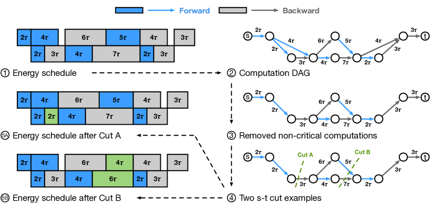
Figure 6: A simplified example of how to reduce iteration time by unit time $\tau$. Given a 1F1B pipeline schedule with 2 stages and 3 microbatches ( ), it is first transformed to an equivalent representation of computation DAG ( ). Then the Critical DAG ( ) is obtained by considering every and only the computations on the critical path. Our key observation is that any valid s-t cut on the Critical DAG will reduce the iteration time by unit time $\tau$. Cut A and Cut B are two examples of valid s-t cut ( ). Either reducing the one computation associated with Cut A ( ) or reducing the two computations associated with Cut B ( ) reduces the iteration time by $\tau$.

In this section, we describe our core subroutine ReduceTime (Algorithm 1, line 1). Figure 6 provides visualizations of the process. The entire procedure is given in Algorithm 2.

Node- and Edge-Centric Computation DAGs.

Originally, Perseus’s representation of the computation DAG is node-centric, which has forward and backward computations as nodes and their dependencies as edges. As a setup for subsequent steps, we convert this into an edge-centric computation DAG where computations are edges and dependencies are nodes (i.e., all incoming edges must complete before any outgoing edge can begin). This conversion can be done by splitting each node on the original computation DAG into two nodes and connecting the two with an edge annotated with the computation on the original node.

Removing Non-Critical Computations.

Our goal is to reduce the execution time of the computation DAG by $\tau$, which is equivalent to reducing the length of all critical paths by $\tau$. Since computations that are not on any critical path (i.e., non-critical computations) do not affect the length of the critical path, we simply remove them from the computation DAG.

Finding Computations to Speed Up.

Which computations on the DAG should we speed up in order to reduce the length of all critical paths by $\tau$? The key observation is that any s-t cut on the computation DAG represents a way to reduce the execution time of the DAG by $\tau$. Specifically, by speeding up the computations on all cut edges by $\tau$, the entire computation DAG can be sped up exactly by $\tau$.

Figure 6 shows two examples of this. We have already transformed an energy schedule into a computation DAG where computations are represented by edges, and removed all non-critical computations. Here, shows two valid s-t cuts: Cut A and Cut B. speeds up the Backward computation cut by Cut A from $3\tau$ to $2\tau$, and the iteration time of the energy schedule was reduced by $\tau$. Similarly, speeds up the Forward computation and Backward computation defined by Cut B from $5\tau$ to $4\tau$ and from $7\tau$ to $6\tau$ respectively, and the iteration time of the energy schedule was also reduced by $\tau$. Especially, in the second case, iteration time was only reduced because computations on two parallel critical paths were sped up together.

Solving with Minimum Cut.

We have shown with examples that any s-t cut represents a way to reduce the duration of the computation DAG by $\tau$. Then, a natural question is, which cut brings the smallest possible energy increase?

We can precisely map the capacity of an s-t cut to the amount of energy increase from speeding up cut edges by finding the amount of energy increase each computation will incur with the slope of the exponential function fit for that computation and defining it to be the edge’s flow capacity. Then, our problem reduces to minimum cut, which we can solve with maximum flow. Appendix D has further details.

Converting to GPU Frequencies.

After finding the minimum capacity (minimum energy increase) cut, we will modify the durations of the computations involved in the cut, which results in a new energy schedule. Finally, we will convert the energy schedule into GPU frequencies that can be realized by the Perseus client. For each computation $i$, we convert its execution time $t$ to the slowest GPU frequency that will execute faster than $t$. This is because when computations are tightly packed by our algorithm, while slightly speeding up a computation is acceptable, slowing down any computation on the critical path will directly slow down the entire DAG, increasing intrinsic energy bloat.

Time Complexity Analysis.

Our optimization algorithm has polynomial runtime. Let $N$ and $M$ respectively denote the number of stages and microbatches. Then, the computation DAG will have $O(NM)$ number of nodes and edges, and maximum flow with Edmonds-Karp runs in $O(N^{3}M^{3})$. While for general DAGs the total number of steps is known to be exponential to the size of the DAG [58], we prove that for DAGs that represent pipeline computations, the number of steps is $O(N+M)$, yielding a final polynomial time complexity of $O((N+M)N^{3}M^{3})$. See Appendix E for proof.

In reality, commonly used number of stages ($N$) are 4 to 8 as too many increase pipeline bubble ratio [43, 14]. The number of microbatches ($M$) is typically around $4N$ [26, 59], but recently with high data parallel degree, far less have been reported even for high-performance settings [14]. As such, the algorithm runtime is negligible in practical scenarios (§6.5), given that large model training time is typically several weeks [48].

1

2 

3

Input: DAG $\mathcal{G}$ with computations $i$
Current energy schedule $p$
Amount of iteration time to reduce $\tau$

Output: Pareto-optimal schedule with reduced time $p^{\prime}$

4

5 

6

Function $\mathrm{ReduceTime}$($\mathcal{G}$, $p$, $\tau$):

       $\triangleright$ Construct edge-centric computation DAG ( )

7       $\mathcal{G}\leftarrow$ Split nodes into two and connect with edge

8       $\mathcal{G}\leftarrow$ Crash bipartite node set to one node

9      

      $\triangleright$ Remove non-critical computations ( )

10       Annotate earliest & latest start times for $\forall i\in\mathcal{G}$

11       for $i\in\mathcal{G}$ do

             $\triangleright$ Critical computations should have zero slack

12             if $i$ has different earliest and latest start then

13                   Remove $i$ from $\mathcal{G}$

14                  

15             end if

16            

17       end for

18      

      $\triangleright$ Find set of computations to modify ( )

19       $S$, $T\leftarrow$ FindMinCut($\mathcal{G}$, $p$)

20      

      $\triangleright$ Modify computation durations ( )

21       $I\leftarrow\{i\mid i\textrm{ in }S-T\textrm{ cut}\}$

22       Modify duration of $\forall i\in I$ by $\tau$

23      

      $\triangleright$ Assign frequencies from planned computation times

24       $p^{\prime}\leftarrow$ $\min f_{i}$ that runs no slower than planned

25      

26      return $p^{\prime}$

27

28

29 

30

Algorithm 2 ReduceTime: Reducing the execution time of a computation DAG by $\tau$ with minimal energy increase.

4.4 Extensions

In this section, we present extensions to our optimization algorithm useful for planning large model training.

Tensor Parallelism.

It is trivial to extend our algorithm to tensor parallelism, another essential ingredient of large model training. The observation is that tensor parallel techniques split operations in equal sizes. Therefore, GPUs that execute different portions of the same operation consume the same amount of time and energy. This allows Perseus to operate only on one tensor parallelism copy for each stage, decide the energy schedule for that copy, and replicate it to other copies in the same stage. We show that Perseus works well for hybrid parallelism in Section 6.4.

Single-Choice Operations.

Apart from computation and blocking on communication, there are other operations in the training pipeline that may take non-trivial latencies. For instance, especially on fast GPUs like A100, loading and copying input data into VRAM or communication over slower links can take considerable latency. However, the time and energy consumption of these operations are not affected by the GPU’s frequency. Perseus can take the latency of such operations into account during planning by abstracting them as a node in the DAG with only one frequency choice.

Other Pipeline Schedules.

There are various schedules for pipeline parallel training, including GPipe [26], 1F1B [42], interleaved 1F1B [56], and early recomputation 1F1B [34]. As long as the computations on the schedule can be expressed as a DAG, Perseus can optimize its energy consumption without modification. If there is stage imbalance, we believe that any pipeline schedule will have intrinsic energy bloat.

5 Implementation

The Perseus server is implemented in 1,500 lines of Python [3]. The client is implemented in 300 lines of Python as a library that can be imported into training frameworks.

As a reference, we have integrated the Perseus client with Merak [34], whose open source implementation takes the best of Megatron-LM [5] for high-performance tensor parallelism for transformer models and DeepSpeed [2] for its generic pipeline execution engine. Activation recomputation [12] is enabled by default to allow large batch sizes to fit in GPUs.

Online Time/Energy Profiler.

While accurate timing measurement is well-supported, modern GPUs (NVIDIA A40, A100, and H100) update their cumulative energy consumption counter [8] only once every 100 ms, which is similar to the timescale of one microbatch computation. This makes energy measurement noisy, and no ground truth is available.

At the very moment the cumulative energy counter increases, its value should be accurate. Therefore, Perseus polls the energy counter in the background and records the timestamp of when the counter increased and its value. Then, collected (time, energy) points are interpolated with a linear line. The main training process only records the start and end timing of each computation, allowing Perseus to match timestamps with the interpolated energy curve to calculate each computation’s energy consumption.

The GPU’s frequency is scanned from the highest to the lowest at iteration granularity. As an optimization, when computation energy increases for five consecutive frequencies, profiling is terminated. Beyond that point, frequencies will consume more time and energy, making them suboptimal.

Asynchronous Frequency Controller.

The controller lives in a separate process that communicates with the main training process through a pipe, because setting the GPU’s frequency through NVML [8] should not block computation on the main process. While pipeline execution engine implementations differ widely, many have separate code blocks for forward and backward. Therefore, the controller exposes one method, set_frequency, which takes either "forward" or "backward" and sets the GPU’s frequency as planned.

6 Evaluation

We evaluate Perseus on five workloads and compare it against EnvPipe and Zeus. Our key findings are the following.

• Perseus can effectively reduce intrinsic and extrinsic energy bloat. Training on real GPUs shows up to 28.5% energy savings using Perseus (§6.2).

• In emulated large-scale training scenarios, Perseus significantly outperforms the baselines by consistently providing up to 30% energy savings. We also observe that there is a tradeoff between energy savings and scale (§6.3).

• Energy bloat reduction was possible because Perseus can enumerate efficient energy schedules on the “iteration time–energy” Pareto frontier (§6.4).

• Perseus reduces energy bloat with low overhead (§6.5).

6.1 Experimental Setup

Testbed.

We run our evaluation workloads in a GPU cluster, where each node is equipped with an AMD EPYC 7513 CPU, 512 GB DRAM, and four NVIDIA A40-48G GPUs. For A100 results, we use the node provided by Chameleon Cloud [30], equipped with two Intel Xeon Platinum 8380 CPUs, 512 GB DRAM, and four NVIDIA A100-80G PCIe GPUs.

Workloads and experiment parameters.

We evaluate Perseus with various workloads spanning from GPT-3 [11], Bloom [66], BERT [15], T5 [51], to Wide-ResNet [69]. We use model variants with 1.3B to 6.7B parameters to run the models in our testbed, and scale them up to 176B parameters in large-scale emulation. We chose the microbatch size and number of microbatches that yield the highest throughput given the global batch size. We use the minimum imbalance stage partitioning method described in Section 2.2 for all workloads. Appendix A lists complete model configurations, parameters, and stage partitioning details.

Baselines.

We mainly compare against two prior works:

• EnvPipe [13] reduces only intrinsic energy bloat while trying to minimize slowdown in pipeline execution. We compare Perseus’s amount of energy bloat reduction against that of EnvPipe (§6.2, §6.3).

• Zeus [68] characterizes the time–energy tradeoff of single GPU training. We compare Perseus’s “iteration time–energy” Pareto frontier against that of Zeus (§6.4).

6.2 Reducing Energy Bloat

We start with overall energy bloat reduction – both intrinsic (§6.2.1) and extrinsic (§6.2.2) – achieved by Perseus and EnvPipe by running various models on our testbed. We compare Perseus against EnvPipe, which reduces energy consumption while trying to minimize slowdown. Both solutions use the same amount of GPU resources.

6.2.1 Intrinsic Energy Bloat Reduction

Model	Energy Savings (%)		Slowdown (%)
	Perseus	EnvPipe	Perseus	EnvPipe
GPT-3 1.3B	13.2	8.8	0.1	0.1
BERT 1.3B	12.9	8.0	0.5	0.0
T5 3B	10.6	7.4	1.3	3.4
Bloom 3B	11.7	8.9	0.2	0.2
Wide-ResNet 1.5B	3.2	3.7	2.3	4.1

(a) Four stage pipeline parallelism on A100 GPUs

Model	Energy Savings (%)		Slowdown (%)
	Perseus	EnvPipe	Perseus	EnvPipe
GPT-3 2.7B	21.1	21.7	0.2	5.6
BERT 1.3B	15.7	16.5	0.0	9.7
T5 3B	28.5	19.3	0.0	0.0
Bloom 3B	22.4	19.9	0.0	0.0
Wide-ResNet 1.5B	20.4	16.5	0.2	0.5

(b) Eight stage pipeline parallelism on A40 GPUs

Table 2: Intrinsic energy reduction and slowdown comparison between Perseus and EnvPipe.

Table 2 compares the energy savings achieved by Perseus’s minimum iteration time energy schedule (leftmost point of the “iteration time–energy” frontier) and that by EnvPipe.

We make two observations regarding Perseus. First, models show varying amounts of energy savings because their stage imbalance vary (Table 1). For instance, unlike other models, Wide-ResNet 1.5B on A100 after minimum imbalance stage partitioning has nearly perfect stage balance, leaving little room for non-critical computations to slow down.

Second, A40 demonstrates more energy savings compared to A100. This is because the dynamic clock frequency range of A100 (210–1410 MHz) is smaller than that of A40 (210–1740 MHz). Thus, tuning down the GPU’s frequency yields a relatively smaller change in computation time and energy compared to those at the maximum frequency. However, we expect the upcoming NVIDIA H100 GPU to have better savings because its maximum frequency is 1755 MHz for the PCIe version and 1980 MHz for SXM [44].

EnvPipe in general provides lower energy savings, primarily due to its assumption that the final stage of a pipeline is always the heaviest, which is not always true. Additionally, it sometimes considerably degrades iteration time because it is not aware of single-choice operations inside the pipeline (§4.4) and can slow down some computations too much.

6.2.2 Intrinsic + Extrinsic Energy Bloat Reduction

Model	Method	Energy Savings (%) given $T^{\prime}/T$
# Params		1.05	1.1	1.2	1.3	1.4	1.5
GPT-3	Perseus	14.7	15.9	15.5	15.0	14.6	14.3
1.3B	EnvPipe	8.7	8.5	8.3	8.1	7.9	7.7
Bloom	Perseus	13.6	15.6	15.2	14.7	14.3	14.0
3B	EnvPipe	8.8	8.7	8.4	8.2	8.0	7.8
BERT	Perseus	14.9	16.9	16.4	15.9	15.5	15.0
1.3B	EnvPipe	7.9	7.8	7.5	7.3	7.1	6.9
T5	Perseus	15.3	18.0	17.9	17.4	16.9	16.5
3B	EnvPipe	8.4	8.2	8.0	7.8	7.6	7.4
Wide-ResNet	Perseus	9.4	12.7	12.6	12.3	12.0	11.6
1.5B	EnvPipe	4.9	4.8	4.7	4.5	4.4	4.3

(a) Four stage pipeline parallelism on A100 GPUs

Model	Method	Energy Savings (%) given $T^{\prime}/T$
# Params		1.05	1.1	1.2	1.3	1.4	1.5
GPT-3	Perseus	24.5	26.0	25.9	25.2	24.6	24.0
2.7B	EnvPipe	22.9	22.6	22.0	21.4	20.9	20.4
Bloom	Perseus	25.5	26.4	25.9	25.2	24.6	24.0
3B	EnvPipe	19.6	19.3	18.8	18.3	17.8	17.4
BERT	Perseus	20.0	22.6	24.1	23.4	22.8	22.2
1.3B	EnvPipe	19.2	18.9	18.3	17.8	17.4	16.9
T5	Perseus	27.9	27.3	26.2	25.2	24.3	23.4
3B	EnvPipe	18.4	18.0	17.3	16.6	16.0	15.4
Wide-ResNet	Perseus	24.3	26.2	26.3	25.7	25.0	24.4
1.5B	EnvPipe	16.4	16.2	15.8	15.4	15.0	14.6

(b) Eight stage pipeline parallelism on A40 GPUs

Table 3: Energy savings of Perseus given varying degrees of straggler slowdown ($T^{\prime}/T$). EnvPipe cannot provide additional savings because it does not consider and cannot be applied to optimize extrinsic bloat.

When stragglers create extrinsic energy bloat, the amount of energy savings for a non-straggler pipeline depends on how much energy reduction its time–energy frontier yields for longer iteration times. Table 3 shows the amount of energy savings given varying degrees of straggler slowdown. As described in Section 3.1, non-stragglers’ iteration time is set to be $\min(T^{*},T^{\prime})$, and energy is reduced from (1) slowing down the pipeline itself and (2) blocking on communication for a shorter amount of time, waiting for the straggler. Slowing down the non-stragglers beyond $T^{*}$ increases total energy consumption; hence, Perseus does not slow down pipelines further than $T^{*}$.

The percentage of energy savings increases for lower $T^{\prime}$ values and slowly wanes when $T^{\prime}>T^{*}$. This reduction is due to longer blocking time. That is, the absolute amount of energy savings in Joules is the largest at $T^{*}$, and constant afterward. However, energy consumption during blocking time ($T^{\prime}-T^{*}$) increases for larger $T^{\prime}$ values, lowering the percentage of energy savings for $T^{\prime}>T^{*}$.

Finally, the point of maximum energy savings is different for each model. This is because different models have different $T^{*}$ values, which is determined by how much each stage’s computation slows down on the minimum-energy frequency.

6.3 Large-Scale Emulation

Because we do not have access to a GPU cluster required to run huge models like GPT-3 175B, we use emulation grounded on fine-grained profiling for large-scale evaluation.

Emulation Methodology.

Total # GPUs	# Pipelines	# Microbatches per Pipelines	Global Batch Size
1024	16	96	1536
2048	32	48
4096	64	24
8192	128	12

Table 4: Experiment parameters for GPT-3 175B and Bloom 176B. Each pipeline has tensor parallel degree 8 and 8 pipeline stages.

We profile the time and energy consumption of each layer (e.g., Transformer decoder) in GPT-3 175B and Bloom 176B in bfloat16 to construct the time and energy profile of each stage. Then, we run our optimization algorithm to obtain a theoretical “iteration time–energy” frontier, and use it to report emulated savings. We evaluate the changes in the amount of energy savings in a strong scaling setup presented in Table 4. We do not consider weak scaling, where per-pipeline batch is constant and increasing the global batch size proportionally, because varying the global batch size can affect the model quality [31, 21]. We find that, compared to actual measurements of smaller scale models on A100, the emulator always underestimates the actual percentage of energy savings by 20.2% on average (see Appendix F for details). Meaning, the savings reported by our emulation can likely be considered an empirical lower bound for actual savings. We used A100 SXM GPUs for the A100 results in this section, which is more representative of large scale scenarios (Appendix G provides PCIe results).

Results Summary.

(a)

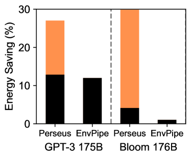
(a)

(b)

Figure 7: Energy savings breakdown of large models emulation with straggler slowdown ($T^{\prime}/T$) 1.20 and 1,024 GPUs.

Figure 7 shows the amount of energy bloat reduction for GPT-3 175B and Bloom 176B large models when slowdown degree is 1.2 on emulated 1,024 GPUs as a representative. EnvPipe can only reduce intrinsic bloat as it does not provide an “iteration time–energy” frontier; even for intrinsic bloat, it reduces less than Perseus. In contrast, Perseus reduces per-iteration energy consumption by up to 30% by reducing both intrinsic and extrinsic energy bloat.

Intrinsic Bloat Reduction.

Model	GPU Type	Energy Savings (%) given # Microbatches
		12	24	48	96
GPT-3 175B	A100	15.20	14.19	13.62	13.32
	A40	11.81	10.22	9.34	8.88
Bloom 176B	A100	10.47	7.06	5.23	4.28
	A40	6.97	4.49	3.12	2.41

Table 5: Perseus’s intrinsic energy bloat reduction of each non-straggler pipeline for GPT-3 175B and Bloom 176B with various number of microbatches. All scenarios run with 8 pipeline stages.

Table 5 presents the changes of intrinsic energy bloat saving of a single pipeline in the case of GPT-3 175B and Bloom 176B with respect to various number of microbatches. For all models, as more and more microbatches are added to the pipeline, the amount of intrinsic bloat decreases. This is fundamentally due to the ratio of microbatches in the pipeline’s warm-up and flush phase (beginning and end) vs. steady state phase (middle). Microbatches in the former phase are able to slow down until their minimum energy frequency, yielding large energy savings. However, microbatches in the latter (middle of the pipeline) cannot slow down to their full potential when the amount of stage imbalance is not large, thereby yielding modest savings. When the number of microbatches in the pipeline increases, only the number of steady state microbatches increases, and energy reduction becomes more and more dominated by the average energy savings of steady state microbatches.

Extrinsic Bloat Reduction.

(a)

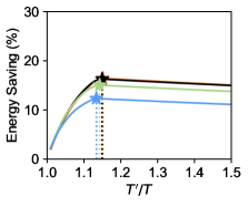
(a)

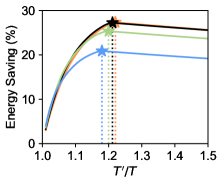
(b)

(c)

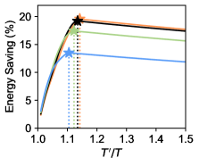
(d)

Figure 8: Perseus’s extrinsic energy savings during a single iteration by slowing down non-straggler pipelines. When $T^{\prime}>T^{*}$, slowing non-stragglers down starts increasing energy consumption, hence non-stragglers do not slow down further than $T^{*}$, whose location is denoted by a star. More blocking time after $T^{*}$ decreases overall energy savings. Please note the different Y-axes.

We simulate stragglers in training large models with hybrid parallelism in various strong scaling configurations (Table 4), where a straggler is slower than others in varying degrees from 1.05 to 1.50. Other non-stragglers, after finishing their computation, must wait until the straggler finishes computation, where extrinsic energy bloat emerges. We measure the amount of energy bloat and Perseus’ extrinsic energy savings.

Figure 8 shows the changes of extrinsic energy bloat reduction given varying degrees of straggler slowdown and various strong scale configurations. The trend where energy saving increases until $T^{\prime}<T^{*}$ and wanes afterward, is consistent with what was observed in Section 6.2.2.

An interesting observation here is that there is a tradeoff between scale and energy savings: more pipelines have less percentage of energy savings or less amount of energy savings per pipeline. It may seem intuitive to assume that more pipelines brings more energy savings, as there is only one straggler pipeline that cannot be optimized while all the other pipelines optimize their energy consumption. However, this holds only in weak-scaling configuration, i.e., per-pipeline batch size is constant (increasing the global batch size proportionally to the number of pipelines) and it is not the case in strong-scaling configuration, where the global batch size is constant and per-pipeline batch size is decreased as more pipelines deployed. With less number of microbatches, the ratio of pipeline bubble (time that GPUs are idle) at the beginning and end of each pipeline iteration, which cannot be eliminated by intrinsic energy bloat reduction, increases, resulting in less energy savings.

6.4 Iteration Time–Energy Frontier Comparison

(a)

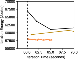
(a)

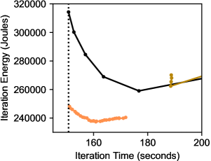
(b)

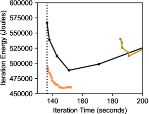
(c)

Figure 9: Iteration time–energy frontiers for GPT-3, achieved by Perseus and the two baselines derived from Zeus [68]. Perseus Pareto-dominates all other approaches. The dotted vertical line is the iteration time of running all GPUs at their maximum power limit, which is the default mode of operation. Please note the different Y-axes.

The energy bloat reductions in Sections 6.2 and 6.3 were made possible by the “iteration time–energy” frontier obtained using Perseus’s optimization algorithm. Here, we further examine the frontier with different parallelization configurations and models and compare against Zeus [68], which is an energy optimization framework for a single-GPU training with the training time–energy frontier. We implemented two Zeus-based baselines to make it work in parallelization configurations and generated “iteration time–energy” frontiers.

1. ZeusGlobal: Scans one global power limit for all stages.

2. ZeusPerStage: Sets one power limit per stage that balances forward computation time.

We run training and measurement under three parallelization configurations: (a) four stage pipeline parallelism on A100; (b) eight stage pipeline parallelism on A40; and (c) hybrid parallelism (data parallelism 2, tensor parallelism 2, pipeline parallelism 4) on A40. Figure 9 shows the frontiers of Perseus and Zeus for different sizes of GPT-3 under three parallelization configurations. Frontiers for other models are in Appendix H.

Perseus Pareto-dominates Zeus. ZeusGlobal is unaware of pipeline stage imbalances and slows down every stage equally, unable to reduce intrinsic energy bloat. While ZeusPerStage can balance the forward computation time of each stage, it is unaware of the critical path of the DAG, slowing down critical computations. In contrast, Perseus can precisely slow down non-critical computations, tightly packing computation.

6.5 Overhead of Perseus

Profiling.

Our online profiling method (§5) introduces extra training time by running some iterations at a lower frequency. For our A100 workloads, the average percentage of slowdown for such iterations was 8.2%, and the average extra training time introduced by profiling was 13 minutes. This is negligible compared to how long large model training can take.

Algorithm Runtime.

The average time spent on running Perseus’s optimization algorithm (§4) across the five A100 workloads was 6.5 minutes, with the longest being Bloom 3B (15.7 minutes). For our largest scale emulation experiment (GPT-3 175B on A100 with 8,192 GPUs), the algorithm ran for 87 seconds. While the runtime of the algorithm will increase with larger DAGs for larger models, we believe the overhead be justified because training time also increases with the scale of the training job. Finding the energy-optimal iteration time and energy schedule given the straggler’s iteration time for extrinsic energy bloat reduction is instant.

7 Related Works

Large Model Training.

Many recent works focus on enabling and accelerating large model training using 3D parallelism (data, tensor, and pipeline parallelism). GPipe [26] and PipeDream [41] were the first to introduce pipeline parallelism and explicitly discussed the difficulty of perfectly balancing computation time across stages. Megatron-LM [56, 43] is a Transformer-based large model training framework that provides efficient manually designed execution plans. Later on, modern training frameworks that focus on large scale training [53, 59, 36, 37, 40, 34] were introduced to support various models at scale. DeepSpeed [53] introduced ZeRO redundancy optimizer that shards model states, which is recently widely used for large model training [52, 72]. Alpa [73] and GSPMD[70] are automatic parallelization framework for general DNNs. Finally, some recent works have looked into fault-tolerant large model training as well [61, 27, 9]. Unfortunately, energy consumption is not an optimization metric for any of the major large model training frameworks.

DNN Training and Energy Consumption.

A recent line of work has highlighted the enormous amount of energy consumption and carbon emission of DNN training, including those that present observations and estimations [48, 60, 33, 16, 38] and those that propose optimization methods for training time, energy consumption, and carbon footprint [74, 63, 68, 67, 32, 13].

Zeus [68] is a recent work that observes the tradeoff between GPU computation time and energy consumption, but focuses on simple single-GPU training. EnvPipe [13], on the other hand, aims to reduce the energy consumption of large model training with minimum slowdown. However, its heuristic assumes that the last pipeline stage is always the bottleneck, leading to suboptimal savings and an infinite loop during optimization. Perseus Pareto-dominates both Zeus and EnvPipe by viewing large model training as a computation DAG and introducing a principled optimization algorithm. Perseus is also the first to introduce the notion of extrinsic energy bloat in large model training and optimize both simultaneously.

8 Conclusion

We presented Perseus, an energy optimization system for large model training. Perseus builds on top of observation that there are fundamental computation imbalance at different levels in large model training that causes intrinsic and extrinsic energy bloat. We introduced a principled graph cut-based algorithm that simultaneously reduces both.

Perseus advances the state-of-the-art of DNN training energy optimization by establishing a new time–energy Pareto frontier for large model training. The integration of Perseus into the training workflow has strong implications for the future of AI development. Importantly, reducing energy bloat leads to practically no latency and throughput degradation, which has the potential to greatly enhance the sustainability of distributed training in the midst of recent proliferation of LLMs and GenAI.

Appendix A Workload Details

A.1 Minimum Imbalance Pipeline Partitioning

Model	Size	Imbalance Ratio		Minimum Imbalance Ratio Partition
		4 stages	8 stages	4 stages	8 stages
GPT-3 [11]	1B	1.17	1.33	[0, 6, 12, 19, 25]	[0, 4, 7, 10, 13, 16, 19, 22, 25]
	3B	1.13	1.25	[0, 8, 16, 25, 33]	[0, 5, 9, 13, 17, 21, 25, 29, 33]
	7B	1.11	1.23	[0, 8, 16, 24, 33]	[0, 4, 8, 12, 16, 20, 24, 28, 33]
	13B	1.08	1.17	[0, 10, 20, 30, 41]	[0, 5, 10, 15, 20, 25, 30, 35, 41]
	175B	1.02	1.03	[0, 24, 48, 72, 97]	[0, 12, 24, 36, 48, 60, 72, 84, 97]
Bloom [66]	3B	1.13	1.25	[0, 9, 17, 25, 31]	[0, 6, 11, 16, 22, 28, 31]
	7B	1.13	1.25	[0, 9, 17, 25, 31]	[0, 6, 11, 16, 22, 28, 31]
	176B	1.05	1.10	[0, 18, 36, 54, 71]	[0, 9, 18, 27, 36, 45, 54, 63, 71]
BERT [15]	0.1B	1.33	2.00	[0, 4, 7, 10, 13]	[0, 2, 3, 4, 6, 8, 10, 12, 13]
	0.3B	1.17	1.33	[0, 7, 13, 19, 25]	[0, 3, 6, 9, 12, 15, 18, 22, 25]
	1.3B	1.17	1.33	[0, 7, 13, 19, 25]	[0, 4, 7, 10, 13, 16, 19, 22, 25]
T5 [51]	0.2B	1.19	1.50	[0, 9, 15, 20, 25]	[0, 5, 9, 13, 15, 17, 19, 22, 25]
	0.7B	1.05	1.11	[0, 16, 29, 39, 49]	[0, 8, 16, 24, 29, 34, 39, 44, 49]
	2.9B	1.06	1.16	[0, 15, 28, 38, 49]	[0, 7, 15, 23, 28, 33, 38, 43, 49]
Wide-ResNet50 [69]	0.8B	1.23	1.46	[0, 5, 9, 14, 18]	[0, 3, 5, 7, 9, 11, 13, 15, 18]
Wide-ResNet101 [69]	1.5B	1.09	1.25	[0, 8, 17, 26, 35]	[0, 4, 8, 12, 16, 21, 26, 31, 35]

(a) NVIDIA A100 PCIe GPUs.

Model	Size	Imbalance Ratio		Minimum Imbalance Ratio Partition
		4 stages	8 stages	4 stages	8 stages
GPT-3 [11]	1B	1.15	1.31	[0, 6, 12, 18, 25]	[0, 3, 6, 9, 12, 15, 18, 21, 25]
	3B	1.11	1.21	[0, 8, 16, 24, 33]	[0, 4, 8, 12, 16, 20, 24, 28, 33]
	7B	1.08	1.17	[0, 8, 16, 24, 33]	[0, 4, 8, 12, 16, 20, 24, 28, 33]
	13B	1.07	1.14	[0, 10, 20, 30, 41]	[0, 5, 10, 15, 20, 25, 30, 35, 41]
	175B	1.01	1.02	[0, 24, 48, 72, 97]	[0, 12, 24, 36, 48, 60, 72, 84, 97]
Bloom [66]	3B	1.13	1.25	[0, 9, 17, 25, 31]	[0, 5, 9, 13, 17, 21, 25, 29, 31]
	7B	1.13	1.25	[0, 9, 17, 25, 31]	[0, 5, 9, 13, 17, 21, 25, 29, 31]
	176B	1.03	1.06	[0, 18, 36, 54, 71]	[0, 9, 18, 27, 36, 45, 54, 63, 71]
BERT [15]	0.1B	1.33	2.00	[0, 4, 7, 10, 13]	[0, 1, 2, 4, 6, 8, 10, 12, 13]
	0.3B	1.17	1.33	[0, 7, 13, 19, 25]	[0, 4, 7, 10, 13, 16, 19, 22, 25]
	1.3B	1.17	1.33	[0, 7, 13, 19, 25]	[0, 3, 6, 9, 12, 15, 18, 22, 25]
T5 [51]	0.2B	1.20	1.50	[0, 9, 15, 20, 25]	[0, 5, 9, 13, 15, 17, 19, 22, 25]
	0.7B	1.06	1.12	[0, 16, 29, 39, 49]	[0, 8, 16, 24, 29, 34, 39, 44, 49]
	2.9B	1.07	1.17	[0, 15, 28, 38, 49]	[0, 8, 15, 23, 28, 33, 38, 43, 49]
Wide-ResNet50 [69]	0.8B	1.13	1.72	[0, 5, 9, 14, 18]	[0, 3, 5, 7, 9, 11, 13, 15, 18]
Wide-ResNet101 [69]	1.5B	1.08	1.25	[0, 8, 17, 26, 35]	[0, 4, 8, 12, 16, 21, 26, 31, 35]

(b) NVIDIA A40 GPUs.

Table 6: Imbalance ratio between the longest and the shortest stages for various models. 1.00 would mean perfect balance. Partitions for $N$ stages is a list of $N+1$ numbers, where the numbers represent layer indices. For instance, [0, 6, 12, 19, 25] for GPT-3 1.3B means there are 6, 6, 7, and 5 Transformer layers in each stage, and the final stage also has the language model head.

We partition layers of a model into $N$ stages such that the imbalance ratio, defined as the ratio of the longest stage forward latency to the shortest, is minimized. We only consider forward computation time as backward computations are typically proportional to forward computation latency. For Transformer-based models, we define layer as one Transformer layer. For Wide-ResNet, we define layer as one Bottleneck layer, which is three convolution layers wrapped with a skip connection. Due to P2P communication overhead and implementation challenges, many planners and frameworks do not support partitioning in the middle of skip connections. We call this minimum imbalance pipeline partitioning, and throughout the paper, every workload we use is partitioned as such.

Table 6 shows the computation time ratios of the heaviest stage to the lightest stage for 4 and 8 pipeline stages. More pipeline stages generally increases imbalance due to the coarse-grained nature of tensor operations. That is, the relative size of each layer becomes smaller and smaller compared to the total amount of computation allocated to each stage, and imbalance increases.

GPT-3, Bloom, and BERT.

Arguably, these are one of the most homogeneous large models because they are a stack of identical Transformer [62] encoder or decoder layers. However, the very last layer is the language modeling head, which maps the final features to probabilities over the entire vocabulary. The vocabulary size of GPT-3 is 50k, Bloom 251k, and BERT 31k, which results in a very large linear layer for the last stage. This leads to varying amounts of imbalance and different minimum imbalance partitioning results for each models.

T5.

This is also based on Transformer layers, but the first half of the layers are encoders, while the later half are decoders (which corresponds to the original Transformer [62] model’s architecture). However, the decoder layers as an extra cross attention layer in the middle, making it computationally heavier. Finally, T5 also ends with a language model head with 32k vocabulary size. However, minimum imbalance partitioning still balances T5 to a reasonable degree, although it cannot be perfectly balanced.

Wide-ResNet.

For Wide-ResNet, in order to make it suitable for large model training evaluation, we used the variant with width factor 8. Wide-ResNet is a collection of Bottleneck layers with three convolutions wrapped with a skip connection, and there are four different sizes of Bottleneck layers laid out sequentially. Therefore, even with minimum imbalance partitioning, it is difficult to perfectly balance stages.

A.2 Experiment Parameters

Model	# Parameters	Global Batch Size	Microbatch Size	# Microbatches
gpt3-6.7b	6.7 B	1024	4	128

Table 7: Experiment Parameters for 3D parallelism experiments on A40 GPUs. Microbatch size is per-pipeline, and there are two data parallel copies of the same pipeline. Thus, global batch size should be calculated as the product of microbatch size and the number of microbatches times two.

Model	# Parameters	Global Batch Size	Microbatch Size	# Microbatches
gpt3-2.7b	2.7 B	1024	4	256
bert-huge-uncased	1.3 B	256	8	32
t5-3b	3.0 B	128	4	32
bloom-3b	3.0 B	512	4	128
wide-resnet101 (width factor 8)	1.5 B	1536	32	48

Table 8: Experiment Parameters for eight-stage pipeline parallelism experiments on A40 GPUs. Model variant names are as described in Torch Vision [45] or Huggingface Hub [65].

Model	# Parameters	Global Batch Size	Microbatch Size	# Microbatches
gpt3-xl	1.3 B	512	4	128
bert-huge-uncased	1.3 B	256	8	32
t5-3b	3.0 B	128	4	32
bloom-3b	3.0 B	512	4	128
wide-resnet101 (width factor 8)	1.5 B	1536	64	24

Table 9: Experiment Parameters for Pipeline Parallelism Experiments on A100 PCIe GPUs. Model variant names are as described in Torch Vision [45] or Huggingface Hub [65].

Tables 7, 8, and 9 list model variant names and experiment parameters for our experiments. Model names and configurations for GPT-3 were taken as is from the original model publication [11]. Especially, model names and configurations for BERT and T5 were directly taken from the Huggingface Hub pretrained model zoo, except for the huge variant of BERT, which we created to have hidden dimension 2048. Wide-ResNet was based on Torch Vision [45] but scaled up following the model’s original publication [69] using its width factor parameter. The unit time parameter $\tau$ was set to 1 ms for all experiments.

Appendix B Pipeline Energy Minimization is NP-Hard

The original Pipeline Energy Minimization problem is stated in formal terms:

$$\min_{F} \textrm{Energy}(F)$$ (6)

s.t. $$\textrm{Time}(F)\leq T^{\prime}$$

where $F$ is the frequency assignment for each pipeline computation $i\in\mathcal{G}$, $T^{\prime}$ is the straggler pipeline’s iteration time. The decision problem corresponding to Equation 6 asks whether it is possible to find frequency assignment $F$ such that the total energy consumption is minimized while the iteration time of pipeline $\mathcal{G}$ is no longer than the straggler’s iteration time. We denote this problem pem.

In the following, we show that a simplification of pem is NP-hard by reduction from the 0/1 Knapsack problem, which makes pem NP-Hard.

B.1 One Stage Two Frequencies Simplification

A simplification of pem is considering the case where there is only one pipeline stage and two frequencies to choose from.

For each pipeline computation $i\in\{1,2,\ldots,n\}$, we can set the GPU frequency to either the lowest value or the highest, denoted as $[L,H]$ respectively. Choosing different frequencies will lead to different execution time and energy consumption. That is, if $i$ is chosen to execute at frequency $L$, it will take $t_{i}(L)$ time and $e_{i}(L)$ energy. On the other hand, if $i$ executes at frequency $H$, it takes $t_{i}(H)$ time and $e_{i}(H)$ energy. The time and energy consumption of $i$ are rational numbers, as they are rounded up to $\tau$.

Our goal is to minimize the energy consumption of executing all computations while satisfying the time constraint. Specifically, given a time deadline $T^{\prime}$, we want to pick a subset of operations $J\subseteq\{1,2,\ldots,n\}$ and assign them to execute at the lowest frequency $L$ and execute the rest of the operations with the highest frequency $H$, such that the total time needed to execute all operations is smaller than or equal to the deadline:

$$\sum^{n}_{i=1}(X_{i}t_{i}(L)+(1-X_{i})t_{i}(H))\leq T^{\prime}$$

where $X_{i}$ is a 0/1 indicator variable where $X_{i}=1$ if $i\in J$ and $X_{i}=0$ otherwise. Under this time constraint, the goal is to minimize the total energy consumption of executing all computations:

$$\sum^{n}_{i=1}(X_{i}e_{i}(L)+(1-X_{i})e_{i}(H)).$$

Formally, we denote this problem as

$$\textsc{pem-1d}(T=(T_{L},T_{H}),E=(E_{L},E_{H}),T^{\prime},EC)$$

where $T_{L}=[t_{1}(L),\ldots,t_{n}(L)]$, $T_{H}=[t_{1}(H),\ldots,t_{n}(H)]$ are execution time vectors for low and high frequency respectively, $E_{L}=[e_{1}(L),\ldots,e_{n}(L)]$, $E_{H}=[e_{1}(H),\ldots,e_{n}(H)]$ are energy consumption vectors for low and high frequency respectively, and $EC$ the target energy consumption.

pem-1d returns true if and only if there exists a subset of operations $J\subseteq\{1,2,\ldots,n\}$ such that $\sum^{n}_{i=1}(X_{i}t_{i}(L)+(1-X_{i})t_{i}(H))\leq T^{\prime}$ and $\sum^{n}_{i=1}(X_{i}e_{i}(L)+(1-X_{i})e_{i}(H))\leq EC$.

B.2 0/1 Knapsack Problem

Consider two length $n$ arrays containing positive integer weights $W=(w_{1},w_{2},\ldots,w_{n})$ and values $V=(v_{1},v_{2},\ldots,v_{n})$ where the $i$th item has weight $w_{i}\in\mathbb{Q}^{+}$ and value $v_{i}\in\mathbb{Q}^{+}$, and a knapsack with weight capacity $C\in\mathbb{Q}^{+}$.

The goal is to pick a subset of items $S\subseteq\{1,2,\ldots,n\}$, such that the total weight of the chosen items is less than or equal to the weight capacity: $\sum_{i\in S}w_{i}\leq C$. Under this constraint, the goal is to maximize the total value of items in the knapsack: $\sum_{i\in S}v_{i}$.

Formally, we denote the decision problem of 0/1 Knapsack as

$$\textsc{knapsack}(W[1,\ldots,n],V[1,\ldots,n],C,P)$$

where $P\in\mathbb{Q}$ is the target value.

knapsack returns true if and only if there exists a subset of items $S\subseteq\{1,2,\ldots,n\}$ such that $\sum_{i\in S}w_{i}\leq C$ and $\sum_{i\in S}v_{i}\geq P$.

It is well known that knapsack is NP-Hard.

B.3 NP-Hardness Proof

Theorem 2.

pem-1d is NP-Hard.

Proof.

We will show that $\textsc{knapsack}\leq_{p}\textsc{pem-1d}$, i.e., the 0/1 Knapsack problem is polynomial-time reducible to the simplified pipeline energy minimization problem. Reduction function $f$ takes $(W[1,\ldots,n],V[1,\ldots,n],C,P)$ as input and does the following:

1. Construct $n$ computations and empty vectors $T_{L},T_{H},E_{L},E_{H}$.

2. For $\forall i$, set $t_{i}(L)=w_{i}$ and append to $T_{L}$.

3. For $\forall i$, set $t_{i}(H)=0$ and append to $T_{H}$.

4. For $\forall i$, set $e_{i}(L)=-v_{i}$ and append to $E_{L}$.

5. For $\forall i$, set $e_{i}(H)=0$ and append to $E_{H}$.

6. Set $T^{\prime}$ = $C$ and $EC$ = $-P$.

7. Output $(T=(T_{L},T_{H}),E=(E_{L},E_{H}),T^{\prime},EC)$

Correctness Analysis

If $(W[1,\ldots,n],V[1,\ldots,n],C,P)\in\textsc{knapsack}$, there exists a subset $S$ such that $\sum_{i\in S}w_{i}\leq C$ and $\sum_{i\in S}v_{i}\geq P$. Now for $\textsc{pem-1d}(T=(T_{L},T_{H}),E=(E_{L},E_{H}),T^{\prime},EC)$, select computations that have the same indices as items in $S$ to execute at low frequency $L$, while executing others at high frequency $H$. Then, for the time constraint, $\sum^{n}_{i=1}(X_{i}t_{i}(L)+(1-X_{i})t_{i}(H))=\sum^{n}_{i=1}X_{i}t_{i}(L)=\sum_{i\in S}w_{i}\leq C=T^{\prime}$, and for target energy, $\sum^{n}_{i=1}(X_{i}e_{i}(L)+(1-X_{i})e_{i}(H))=\sum^{n}_{i=1}X_{i}e_{i}(L)=\sum_{i\in S}-v_{i}\leq-P=EC$.

If $(W[1,\ldots,n],V[1,\ldots,n],C,P)\notin\textsc{knapsack}$, there does not exist a subset $S$ such that $\sum_{i\in S}w_{i}\leq C$ and $\sum_{i\in S}v_{i}\geq P$. There are two possibilities: either a subset $S$ that satisfies the weight constraint does not exist at all ($w_{i}>C,\forall i$) or none of the subsets $S$ that satisfy the weight constraint satisfy $\sum_{i\in S}v_{i}\geq P$. For the first possibility, this means all the computations must select the high frequency as the low frequency does not satisfy the time constraint. Then total energy consumption is 0, which is larger than $EC=-P$ since $P\in\mathbb{Q}^{+}$. For the second possibility, for all subsets $S$, $\sum_{i\in S}v_{i}<P$, which means that for all subsets of computations $\sum^{n}_{i=1}(X_{i}e_{i}(L)+(1-X_{i})e_{i}(H))=\sum_{i\in S}-v_{i}>-P=EC$, so none of them satisfy the energy constraint.

Efficiency Analysis

Step 1–5 each takes $O(n)$ time. Step 6 takes $O(1)$ time. Finally, step 7 takes $O(n)$ time.

Therefore, the function $f$ takes $O(n)$ time, which is polynomial time w.r.t the input size.

∎

Appendix C Visualizations for Intrinsic Energy Bloat

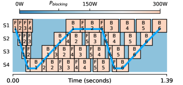
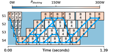
(a)

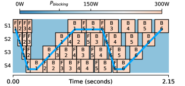
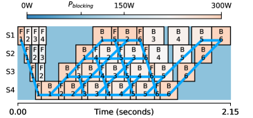
(b)

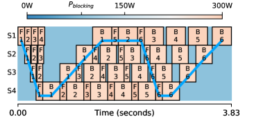
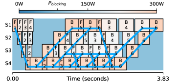
(c)

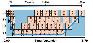
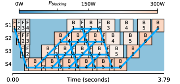
(d)

Figure 10: Visualization of Perseus’s solution for four stage pipeline workloads on NVIDIA A100 PCIe GPUs. For each workload, the left is running every computation at maximum frequency, and the right is Perseus’s energy schedule that reduces only intrinsic energy bloat without inflating iteration time. Note that these are not real workloads we run in Section 6; real workloads have far more microbatches.

Figure 10 shows the timeline of running one training iteration of BERT 1.3B, T5 3B, Bloom 3B, and Wide-ResNet101 1.5B for maximum frequency and Perseus-optimized energy schedule, respectively. For visualization purposes, we set the number of microbatches to 6. Real evaluation workloads have more microbatches. Energy schedule found by Perseus successfully tunes down frequency for all models without slowing down the iteration time, tightly packing computations over time and reducing intrinsic energy bloat.

Appendix D Full Details of ReduceTime

For the sake of presentation, we made a simplifying statement in the body of the paper that computations only speed up by $\tau$. However, since we aim to speed up all critical paths by precisely $\tau$, speeding up more than one computation from a critical path allows other computations on that critical path to be slowed down. We always take such slowdown opportunity because it will decrease energy consumption.

In the following, we describe the procedure of annotating edges with flow capacities and then solving the problem with maximum flow.

D.1 Generating Capacity DAG

On the computation DAG, we first remove all the computations that are not on any of the critical paths and construct the Critical DAG. We would like to find a set of edges $I^{+}$ to speed up by $\tau$ and $I^{-}$ to slow down by $\tau$ on the Critical DAG, such that the total energy consumption increases minimally. This can be described as the following problem:

$$\min_{I^{+},\leavevmode\nobreak\ I^{-}}\quad\sum_{i\in I^{+}}{e_{i}^{+}}-\sum_{i\in I^{-}}{e_{i}^{-}},$$ (7)

where $e_{i}(t_{i})$ is the exponential function fit to Pareto-optimal (time, energy) measurments for computation $i$, $e_{i}^{+}=e_{i}(t_{i}-\tau)-e_{i}(t_{i})$ is the extra amount of energy needed to speed up $i$ by $\tau$ and $e_{i}^{-}=e_{i}(t_{i})-e_{i}(t_{i}+\tau)$ is the energy saved from slowing down $i$ by $\tau$.

An important fact that leads us to the solution is that (i) the problem of finding the set of edges to modify such that energy increase is minimized (i.e., solving Equation 7) coincides with (ii) finding the minimum cut of a DAG whose lower and upper bound flow capacities are defined as

$$(l_{i},u_{i})=\begin{cases}(0,e_{i}^{+})&\textrm{if }t_{i}\textrm{ is longest possible (slowest)}\\ (e_{i}^{-},\infty)&\textrm{if }t_{i}\textrm{ is shortest possible (fastest)}\\ (e_{i}^{-},e_{i}^{+})&\textrm{otherwise.}\end{cases}$$ (8)

This equivalence was discovered by Phillips and Dessouky [49, 24].

Thus, we construct the Capacity DAG from the Critical DAG by annotating its edges with flow capacities given by Equation 8. The capacity of an $S-T$ cut ($S$ is the set of nodes on the source side and $T$ the sink side) on the Capacity DAG with $S\rightarrow T$ edges $I^{+}$ and $T\rightarrow S$ edges $I^{-}$ is identical to the objective in Equation 7. Then, we use the Edmonds-Karp maximum flow algorithm [17] to find the minimum cut of the Capacity DAG. Finally, after the minimum cut has been identified from the Capacity DAG, edges in $I^{+}$ are sped up by $\tau$ and those in $I^{-}$ are slowed down by $\tau$, ultimately reducing the length of every critical path exactly by $\tau$ with the smallest possible energy increase.

D.2 Max Flow Algorithm on the Capacity DAG

A characteristic of our Capacity DAG that precludes the direct application of well-known max flow algorithms is that some edges also have flow lower bounds, asserting that at least a certain amount of flow must pass through in the edge. However, the Max Flow Min Cut theorem by Ford and Fulkerson holds for the case of non-zero flow lower bounds (See Chapter 1, Section 9 of [20]), allowing us to find the minimum cut (which is equivalent to the minimum energy modification set) using any maximum flow algorithm. We adopt an approach that adds dummy source/sink nodes to create a DAG that has zero flow lower bounds, finds the maximum flow on the new DAG, and extracts the flow so that it corresponds to a flow in the original DAG [18]. The algorithm is given in Algorithm 3.

1

2 

3

4

Input: Directed Acyclic Graph $G=(V,E)$
Source node $s\in V$ and sink node $t\in V$
Lower and upper bounds $l(e)$, $u(e)$ for $\forall e\in E$

Output: A maximum feasible flow of $G$ if it exists

5

6 

7

8Construct a new graph $G^{\prime}=(V^{\prime},E^{\prime})$ by adding new source and sink nodes $s^{\prime}$ and $t^{\prime}$, edges from $s^{\prime}$ to each node in $V$, edges from each node in $V$ to $t^{\prime}$, and an edge from $t$ to $s$

9

$\triangleright$ Define the capacity $c^{\prime}(e)$ of each edge $e\in E^{\prime}$

10: for $v\in V$ do

11       $c^{\prime}(s^{\prime}v)\leftarrow\sum_{u\in V}l(uv)$

12       $c^{\prime}(vt^{\prime})\leftarrow\sum_{w\in V}l(vw)$

13      

14 end for

15for $uv\in E$ do

16       $c^{\prime}(uv)\leftarrow u(uv)-l(uv)$

17      

18 end for

19$c^{\prime}(ts)\leftarrow\infty$

20

$\triangleright$ Find the max flow on G’

21 $f^{\prime}\leftarrow$ EdmondsKarp ($G^{\prime}$, $c^{\prime}$)

22

$\triangleright$ $G$ has a feasible flow if and only if $G^{\prime}$ has a saturating flow

23 if FlowValue ($f^{\prime}$) $\neq\sum_{v\in V}{c^{\prime}(s^{\prime}v)}$ then

24       return nil

25      

26 end if

27

$\triangleright$ Convert $f^{\prime}$ to a feasible flow $f$ in $G$

28 for $uv\in E$ do

29       $f(uv)\leftarrow f^{\prime}(uv)+l(uv)$

30      

31 end for

32

$\triangleright$ Construct residual graph and improve $f$ to max flow

33 for $uv\in E$ do

34       $c(uv)\leftarrow u(uv)-f(uv)$

35       $c(vu)\leftarrow f(vu)-l(vu)$

36      

37 end for

38return EdmondsKarp ($G$, $c$)

39

40 

41

Algorithm 3 Maximum Flow with Lower Bounds

Appendix E Proof for Polynomial Runtime

Perseus enumerates the entire “iteration time–energy” Pareto frontier one by one, and the runtime of one iteration is polynomial time with respect to the number of stages $N$ and the number of microbatches $M$. Thus, determining whether the entire algorithm runs in polynomial time reduces to whether the worst case number of iterations is polynomial with respect to $N$ and $M$. While for general DAGs the maximum number of points on the Pareto frontier can be exponential with respect to the size of the DAG [58], here we prove that under mild assumptions for DAGs that represent pipeline schedules, the number of iterations is $O(N+M)$. The assumptions are valid for all pipeline schedules known to the authors, including GPipe [26] and 1F1B [42].

Theorem 3.

For DAGs that represent pipeline schedules, the number of iterations needed is $O(N+M)$.

Proof.

Since we always reduce iteration time by $\tau$, the number of iterations is

$$\frac{t_{\max}-t_{\min}}{\tau}$$

where $t_{\max}$ and $t_{\min}$ are the maximum and minimum possible iteration time, respectively.

Assume that any pipeline schedule representing one iteration of training has a prologue, a steady state, and an epilogue. The prologue is when the pipeline starts from an empty state and is gradually filled with pipeline computations, while the epilogue is when the pipeline is drained to reach an empty state. It is easy to see that the number of pipeline computations on the critical path of both the prologue and epilogue is $O(N)$, as deeper pipelines (larger $N$) take longer to fill. On the other hand, the steady state of the pipeline is when the pipeline is completely filled, and the number of pipeline computations in any simple path through the steady state of the DAG is $O(M)$. Therefore, the total number of pipeline computations in the critical path of the entire DAG is $O(N+M)$.

$t_{\max}$ and $t_{\min}$ can be constructed by multiplying the number of computations with the average execution time of an computation. Computations are executed with frequencies $f_{\min}$ and $f_{\max}$, respectively, and thus the multipliers of $N$ and $M$ do not cancel out when $t_{\max}-t_{\min}$ is evaluated. Therefore, $t_{\max}-t_{\min}$, and hence $(t_{\max}-t_{\min})/\tau$, is $O(N+M)$. ∎

Appendix F Underestimations of the Emulator

Model	Leftmost point	Rightmost point
gpt3-xl	20.5%	23.6%
bert-huge-uncased	26.7%	35.3%
t5-3b	19.1%	19.1%
bloom-3b	9.3%	10.7%
wide-resnet101 (width factor 8)	17.5%	19.8%

Table 10: By how much the emulator underestimates the percentage of energy savings for four-stage pipeline workloads on A100 PCIe. Leftmost point represents intrinsic energy bloat, whereas the rightmost point extrinsic.

Our emulator, used to present energy saving results for large scale workloads (GPT-3 175B and Bloom 176B), always underestimates energy savings compared to actual measurements, and argue that the emulated results are empirically a lower bound of actual savings. The characteristics of time and energy changes depends more on the type of the GPU than the parallelization setting as different GPU generations show drastically different sensitivity in terms of time and energy when frequency is varied. Therefore, we compare results from the A100 PCIe GPU.

Table 10 shows the percentage of energy savings underestimation for two points on the “iteration time–energy” frontier:

• Leftmost point: The point with the shortest iteration time, corresponding to how much the emulator underestimates the amount of possible intrinsic energy bloat reduction.

• Rightmost point: The point with the longest iteration time, corresponding to how much the emulator underestimates the amount of possible energy savings brought about by slowing down the entire pipeline in the case of a straggler.

We believe that underestimation is happening due to our simplifying assumption that $P_{\mathrm{blocking}}$, the power consumption of the GPU while blocking on communication, is constant regardless of the GPU’s frequency. In reality, $P_{\mathrm{blocking}}$ would be an increasing function of frequency. Therefore, when the emulator assumes a constant $P_{\mathrm{blocking}}$ when calculating the energy consumption of a pipeline that is overall running on a reduced frequency, it will be overestimating its total energy consumption, leading to underestimations.

Appendix G Large-Scale Emulation

Section 6.3 used A100 SXM GPUs, which we momentarily had access to, in order to profile model layers and run large scale emulation. This is because we believe that SXM models are more representative of real large scale GPU clusters that train large models. Nonetheless, in this section, we provide the same set of results from A100 PCIe GPUs, as well, along with the same A40 GPUs results. All other experiment methodology and parameters are identical.

Results Summary.

(a)

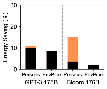
(a)

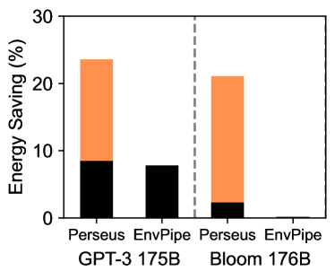
(b)

Figure 11: Energy savings breakdown of large models emulation with straggler slowdown ($T^{\prime}/T$) 1.20 and 1024 GPUs.

Figure 11 shows the amount of energy bloat reduction for GPT-3 175B and Bloom 176B large models when slowdown degree is 1.2 on emulated 1024 GPUs as a representative.

Intrinsic Bloat Reduction.

Model	GPU Type	Energy Savings (%) given # Microbatches
		12	24	48	96
GPT-3 175B	A100	9.02	9.77	10.17	10.39
	A40	11.81	10.22	9.34	8.88
Bloom 176B	A100	6.39	4.99	4.21	3.80
	A40	6.97	4.49	3.12	2.41

Table 11: Perseus’s intrinsic energy bloat reduction of each non-straggler pipeline for GPT-3 175B and Bloom 176B with various number of microbatches. All scenarios run with 8 pipeline stages.

Table 11 presents the changes of intrinsic energy bloat saving of a single pipeline in the case of GPT-3 175B and Bloom 176B with respect to various number of microbatches. GPT-3 175B on A100 is unique and has the opposite trend compared to others: intrinsic energy bloat reduction increases with the number of microbatches. The opposite trends stem from the amount of stage imbalance on each GPU, and the amount of slowdown the minimum-energy frequency incurs. What is unique about GPT-3 175B on A100 is that the amount of imbalance is large whereas the minimum-energy frequency incurs little slowdown for forward and backward computations. Therefore, only for GPT-3 175B on A100, microbatches in the middle of the pipeline are able to fully slow down to their potential. Thus, when such microbatches are added to the pipeline, the percentage of intrinsic energy bloat reduction increases.

Extrinsic Energy Bloat.

(a)

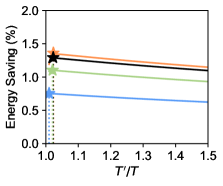
(a)

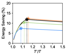
(b)

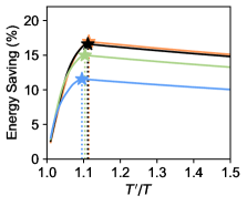
(c)

(d)

Figure 12: Perseus’s extrinsic energy savings during a single iteration by slowing down non-straggler pipelines. When $T^{\prime}>T^{*}$, slowing non-stragglers down starts increasing energy consumption, hence non-stragglers do not slow down further than $T^{*}$. More blocking time after $T^{*}$ decreases overall energy savings. Please note the different Y-axes.

Figure 12 presents extrinsic energy bloat results in the strong scaling configuration, where a straggler is slower than others in varying degrees of slowdown from 1.05 to 1.50.

Appendix H Iteration Time–Energy Frontiers

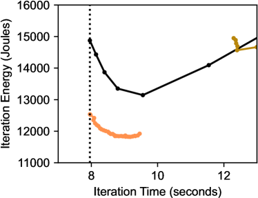
(a) BERT

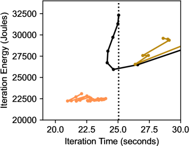
(b) T5

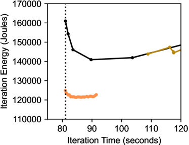
(c) Bloom

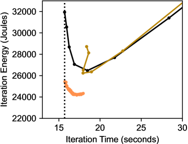
(d) Wide-ResNet

Figure 13: Eight stage pipeline parallelism on A40.

Figure 13 shows the “iteration time–energy” frontiers achieved by Perseus and the two baseline approaches for the rest of the workloads ran with eight stage pipeline parallelism, measured in NVIDIA A40 GPUs.

T5 shows an interesting frontier due to the hardware topology of our A40 machine setup: Each node has four GPUs and NVLink connects GPUs 0 and 1, and 2 and 3; GPUs 1 and 2 must communicate through the NUMA interconnect; Finally, different nodes are connected with Infiniband only adjacent to GPUs 0 and 1 (data to and from GPUs 2 and 3 must also go through the NUMA interconnect). The implication of this heterogeneous GPU interconnect is that if more than one P2P communications that need to go through the NUMA interconnect happen at the same time, contention happens and both of data transfers slow down significantly. However, Perseus’s plan reduces this contention, overall decreasing iteration time noticeably. Yet, contention and noisy communication latencies still exist, leading to a noisy frontier.

For many ZeusPerStage lines, energy fluctuates significantly when iteration time increases due to ZeusPerStage being unaware of critical paths. Balancing the forward computation time between stages could even let the modified stages take over the critical path. As a result, the iteration time increases, which increases energy bloat, and more energy is spent on blocking on communication (§4.1). When the decreased energy on computation fails to cover the increased energy on P2P communication, total energy increases.

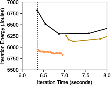
(a) BERT

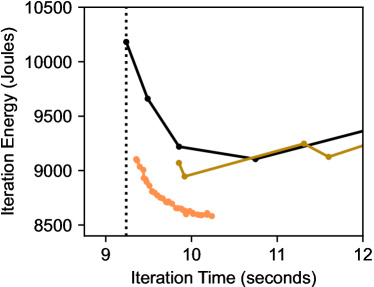
(b) T5

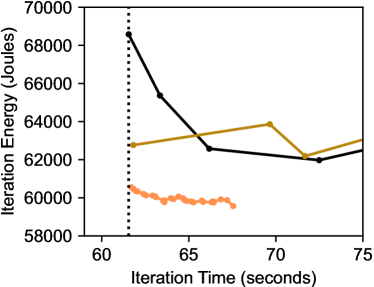
(c) Bloom

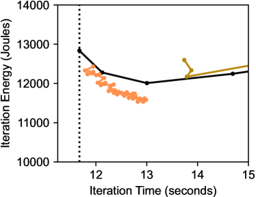
(d) Wide-ResNet

Figure 14: 4 stage pipeline parallelism on A100 PCIe.

Figure 14 shows the “iteration time–energy” frontiers achieved by Perseus and the two baseline approaches for the rest of the workloads, measured with four stage pipeline parallelism in NVIDIA A100 PCIe GPUs. Wide-ResNet has a noisy frontier because the variability in microbatch loading time introduces noise in the end-to-end iteration time when computations are tightly packed by Perseus. This was not pronounced in A40 GPUs because compared to A100 PCIe, computation is slower, but data loading time is similar. Thus, the noise in data loading time becomes more noticeable in A100 PCIe.

References

- [1] Apple environment. https://www.apple.com/environment.
- [2] DeepSpeed. https://github.com/microsoft/DeepSpeed.
- [3] FastAPI. https://github.com/tiangolo/fastapi.
- [4] Google sustainability. https://sustainability.google.
- [5] Megatron-LM. https://github.com/NVIDIA/Megatron-LM.
- [6] Meta climate. https://sustainability.fb.com/climate.
- [7] Microsoft sustainability. https://www.microsoft.com/en-us/sustainability.
- [8] NVIDIA Management Library (NVML). https://developer.nvidia.com/nvidia-management-library-nvml.
- [9] Sanjith Athlur, Nitika Saran, Muthian Sivathanu, Ramachandran Ramjee, and Nipun Kwatra. Varuna: Scalable, low-cost training of massive deep learning models. In EuroSys, 2022.
- [10] Emily M. Bender, Timnit Gebru, Angelina McMillan-Major, and Shmargaret Shmitchell. On the dangers of stochastic parrots: Can language models be too big? In Proceedings of the 2021 ACM Conference on Fairness, Accountability, and Transparency (FAccT ’21), 2021.
- [11] Tom Brown, Benjamin Mann, Nick Ryder, Melanie Subbiah, Jared D Kaplan, Prafulla Dhariwal, Arvind Neelakantan, Pranav Shyam, Girish Sastry, Amanda Askell, Sandhini Agarwal, Ariel Herbert-Voss, Gretchen Krueger, Tom Henighan, Rewon Child, Aditya Ramesh, Daniel Ziegler, Jeffrey Wu, Clemens Winter, Chris Hesse, Mark Chen, Eric Sigler, Mateusz Litwin, Scott Gray, Benjamin Chess, Jack Clark, Christopher Berner, Sam McCandlish, Alec Radford, Ilya Sutskever, and Dario Amodei. Language models are few-shot learners. In NeurIPS, 2020.
- [12] Tianqi Chen, Bing Xu, Chiyuan Zhang, and Carlos Guestrin. Training deep nets with sublinear memory cost. 2016.
- [13] Sangjin Choi, Inhoe Koo, Jeongseob Ahn, Myeongjae Jeon, and Youngjin Kwon. EnvPipe: Performance-preserving DNN training framework for saving energy. In ATC, 2023.
- [14] ML COMMONS. MLPerf training v3.1 benchmark results. https://github.com/mlcommons/training_results_v3.1.
- [15] Jacob Devlin, Ming-Wei Chang, Kenton Lee, and Kristina Toutanova. BERT: Pre-training of deep bidirectional transformers for language understanding. In Proceedings of the 2019 Conference of the North American Chapter of the Association for Computational Linguistics (NAACL), 2019.
- [16] Jesse Dodge, Taylor Prewitt, Remi Tachet des Combes, Erika Odmark, Roy Schwartz, Emma Strubell, Alexandra Sasha Luccioni, Noah A. Smith, Nicole DeCario, and Will Buchanan. Measuring the carbon intensity of ai in cloud instances. In 2022 ACM Conference on Fairness, Accountability, and Transparency, 2022.
- [17] Jack Edmonds and Richard M. Karp. Theoretical improvements in algorithmic efficiency for network flow problems. Journal of the ACM, 19(2):248–264, 1972.
- [18] Jeff Erickson. Extensions of maximum flow. https://courses.engr.illinois.edu/cs498dl1/sp2015/notes/25-maxflowext.pdf. [Online; accessed 05-April-2023].
- [19] Shiqing Fan, Yi Rong, Chen Meng, Zongyan Cao, Siyu Wang, Zhen Zheng, Chuan Wu, Guoping Long, Jun Yang, Lixue Xia, Lansong Diao, Xiaoyong Liu, and Wei Lin. DAPPLE: A pipelined data parallel approach for training large models. In ACM PPoPP, 2021.
- [20] L. R. Ford and D. R. Fulkerson. Flows in Networks. Princeton University Press, 1962.
- [21] Noah Golmant, Nikita Vemuri, Zhewei Yao, Vladimir Feinberg, Amir Gholami, Kai Rothauge, Michael W Mahoney, and Joseph Gonzalez. On the computational inefficiency of large batch sizes for stochastic gradient descent. arXiv preprint arXiv:1811.12941, 2018.
- [22] Saurabh Gupta, Tirthak Patel, Christian Engelmann, and Devesh Tiwari. Failures in large scale systems: Long-term measurement, analysis, and implications. In SC, 2017.
- [23] Chaoyang He, Shen Li, Mahdi Soltanolkotabi, and Salman Avestimehr. PipeTransformer: Automated elastic pipelining for distributed training of large-scale models. In ICML, 2021.
- [24] Dorit S. Hochbaum. A polynomial time repeated cuts algorithm for the time cost tradeoff problem: The linear and convex crashing cost deadline problem. Computers & Industrial Engineering, 95:64–71, 2016.
- [25] Jordan Hoffmann, Sebastian Borgeaud, Arthur Mensch, Elena Buchatskaya, Trevor Cai, Eliza Rutherford, Diego de Las Casas, Lisa Anne Hendricks, Johannes Welbl, Aidan Clark, Thomas Hennigan, Eric Noland, Katherine Millican, George van den Driessche, Bogdan Damoc, Aurelia Guy, Simon Osindero, Karén Simonyan, Erich Elsen, Oriol Vinyals, Jack Rae, and Laurent Sifre. An empirical analysis of compute-optimal large language model training. In NeurIPS, 2022.
- [26] Yanping Huang, Youlong Cheng, Ankur Bapna, Orhan Firat, Mia Xu Chen, Dehao Chen, HyoukJoong Lee, Jiquan Ngiam, Quoc V. Le, Yonghui Wu, and Zhifeng Chen. GPipe: Efficient training of giant neural networks using pipeline parallelism. In NeurIPS, 2019.
- [27] Insu Jang, Zhenning Yang, Zhen Zhang, Xin Jin, and Mosharaf Chowdhury. Oobleck: Resilient distributed training of large models using pipeline templates. In SOSP, 2023.
- [28] Myeongjae Jeon, Shivaram Venkataraman, Amar Phanishayee, Junjie Qian, Wencong Xiao, and Fan Yang. Analysis of Large-Scale Multi-Tenant GPU clusters for DNN training workloads. In ATC, 2019.
- [29] Jared Kaplan, Sam McCandlish, Tom Henighan, Tom B. Brown, Benjamin Chess, Rewon Child, Scott Gray, Alec Radford, Jeffrey Wu, and Dario Amodei. Scaling laws for neural language models. arXiv preprint arXiv:2001.08361, 2020.
- [30] Kate Keahey, Jason Anderson, Zhuo Zhen, Pierre Riteau, Paul Ruth, Dan Stanzione, Mert Cevik, Jacob Colleran, Haryadi S Gunawi, Cody Hammock, et al. Lessons learned from the chameleon testbed. In ATC, 2020.
- [31] Nitish Shirish Keskar, Dheevatsa Mudigere, Jorge Nocedal, Mikhail Smelyanskiy, and Ping Tak Peter Tang. On large-batch training for deep learning: Generalization gap and sharp minima. In ICLR, 2017.
- [32] Adam Krzywaniak, Paweł Czarnul, and Jerzy Proficz. Dynamic GPU power capping with online performance tracing for energy efficient GPU computing using DEPO tool. Future Generation Computer Systems, 145:396–414, 2023.
- [33] Alexandre Lacoste, Alexandra Luccioni, Victor Schmidt, and Thomas Dandres. Quantifying the carbon emissions of machine learning. arXiv preprint arXiv:1910.09700, 2019.
- [34] Zhiquan Lai, Shengwei Li, Xudong Tang, Keshi Ge, Weijie Liu, Yabo Duan, Linbo Qiao, and Dongsheng Li. Merak: An efficient distributed DNN training framework with automated 3d parallelism for giant foundation models. IEEE Transactions on Parallel and Distributed Systems, 34(5):1466–1478, 2023.
- [35] Shaohong Li, Xi Wang, Xiao Zhang, Vasileios Kontorinis, Sreekumar Kodakara, David Lo, and Parthasarathy Ranganathan. Thunderbolt: Throughput-Optimized, Quality-of-Service-Aware power capping at scale. In OSDI, 2020.
- [36] Shenggui Li, Hongxin Liu, Zhengda Bian, Jiarui Fang, Haichen Huang, Yuliang Liu, Boxiang Wang, and Yang You. Colossal-ai: A unified deep learning system for large-scale parallel training. In Proceedings of the 52nd International Conference on Parallel Processing, ICPP ’23, page 766–775, New York, NY, USA, 2023. Association for Computing Machinery.
- [37] Lightning-AI. Pytorch lightning. https://lightning.ai/pytorch-lightning.
- [38] Alexandra Sasha Luccioni, Sylvain Viguier, and Anne-Laure Ligozat. Estimating the carbon footprint of BLOOM, a 176b parameter language model. 2022.
- [39] Jayashree Mohan, Amar Phanishayee, Ashish Raniwala, and Vijay Chidambaram. Analyzing and mitigating data stalls in dnn training. 14(5):771–784, jan 2021.
- [40] MosaicML. Mosaicml training. https://www.mosaicml.com/training.
- [41] Deepak Narayanan, Aaron Harlap, Amar Phanishayee, Vivek Seshadri, Nikhil R Devanur, Gregory R Ganger, Phillip B Gibbons, and Matei Zaharia. PipeDream: generalized pipeline parallelism for DNN training. In SOSP, 2019.
- [42] Deepak Narayanan, Amar Phanishayee, Kaiyu Shi, Xie Chen, and Matei Zaharia. Memory-efficient pipeline-parallel DNN training. In ICML, 2021.
- [43] Deepak Narayanan, Mohammad Shoeybi, Jared Casper, Patrick LeGresley, Mostofa Patwary, Vijay Korthikanti, Dmitri Vainbrand, Prethvi Kashinkunti, Julie Bernauer, Bryan Catanzaro, Amar Phanishayee, and Matei Zaharia. Efficient large-scale language model training on GPU clusters using Megatron-LM. In SC, 2021.
- [44] NVIDIA. Nvidia H100 tensor core GPU architecture overview. https://resources.nvidia.com/en-us-tensor-core/gtc22-whitepaper-hopper.
- [45] Adam Paszke, Sam Gross, Francisco Massa, Adam Lerer, James Bradbury, Gregory Chanan, Trevor Killeen, Zeming Lin, Natalia Gimelshein, Luca Antiga, et al. Pytorch: An imperative style, high-performance deep learning library. NeurIPS, 2019.
- [46] Pratyush Patel, Esha Choukse, Chaojie Zhang, Íñigo Goiri, Brijesh Warrier, Nithish Mahalingam, and Ricardo Bianchini. POLCA: Power oversubscription in llm cloud providers. 2023.
- [47] Pratyush Patel, Zibo Gong, Syeda Rizvi, Esha Choukse, Pulkit Misra, Thomas Anderson, and Akshitha Sriraman. Towards improved power management in cloud gpus. IEEE Computer Architecture Letters, 22(2):141–144, 2023.
- [48] David Patterson, Joseph Gonzalez, Quoc Le, Chen Liang, Lluis-Miquel Munguia, Daniel Rothchild, David So, Maud Texier, and Jeff Dean. Carbon emissions and large neural network training. arXiv preprint arXiv:2104.10350, 2021.
- [49] Steve Phillips and Mohamed I. Dessouky. Solving the project time/cost tradeoff problem using the minimal cut concept. Management Science, 24(4):393–400, 1977.
- [50] United Nations Environment Programme. Emissions gap report 2023. https://www.unep.org/resources/emissions-gap-report-2023.
- [51] Colin Raffel, Noam Shazeer, Adam Roberts, Katherine Lee, Sharan Narang, Michael Matena, Yanqi Zhou, Wei Li, and Peter J. Liu. Exploring the limits of transfer learning with a unified text-to-text transformer. Journal of Machine Learning Research, 21(140):1–67, 2020.
- [52] Samyam Rajbhandari, Jeff Rasley, Olatunji Ruwase, and Yuxiong He. ZeRO: Memory optimizations toward training trillion parameter models. In International Conference for High Performance Computing, Networking, Storage and Analysis (SC), 2020.
- [53] Jeff Rasley, Samyam Rajbhandari, Olatunji Ruwase, and Yuxiong He. Deepspeed: System optimizations enable training deep learning models with over 100 billion parameters. In Proceedings of the 26th ACM SIGKDD International Conference on Knowledge Discovery & Data Mining, pages 3505–3506, 2020.
- [54] Varun Sakalkar, Vasileios Kontorinis, David Landhuis, Shaohong Li, Darren De Ronde, Thomas Blooming, Anand Ramesh, James Kennedy, Christopher Malone, Jimmy Clidaras, and Parthasarathy Ranganathan. Data center power oversubscription with a medium voltage power plane and Priority-Aware capping. In ASPLOS, 2020.
- [55] Roy Schwartz, Jesse Dodge, Noah A. Smith, and Oren Etzioni. Green AI. Commun. ACM, 63(12):54–63, 2020.
- [56] Mohammad Shoeybi, Mostofa Patwary, Raul Puri, Patrick LeGresley, Jared Casper, and Bryan Catanzaro. Megatron-LM: Training multi-billion parameter language models using model parallelism. arXiv preprint arXiv:1909.08053, 2019.
- [57] Martin Skutella. Approximation algorithms for the discrete time-cost tradeoff problem. Mathematics of Operations Research, 23(4):909–929, 1998.
- [58] Martin Skutella. Approximation and randomization in scheduling. PhD thesis, 1998.
- [59] Shaden Smith, Mostofa Patwary, Brandon Norick, Patrick LeGresley, Samyam Rajbhandari, Jared Casper, Zhun Liu, Shrimai Prabhumoye, George Zerveas, Vijay Korthikanti, Elton Zhang, Rewon Child, Reza Yazdani Aminabadi, Julie Bernauer, Xia Song, Mohammad Shoeybi, Yuxiong He, Michael Houston, Saurabh Tiwary, and Bryan Catanzaro. Using deepspeed and megatron to train Megatron-Turing NLG 530b, a Large-Scale generative language model. 2022.
- [60] Emma Strubell, Ananya Ganesh, and Andrew McCallum. Energy and policy considerations for deep learning in NLP. Proceedings of the 57th Annual Meeting of the Association for Computational Linguistics, 2019.
- [61] John Thorpe, Pengzhan Zhao, Jonathan Eyolfson, Yifan Qiao, Zhihao Jia, Minjia Zhang, Ravi Netravali, and Guoqing Harry Xu. Bamboo: Making preemptible instances resilient for affordable training of large DNNs. In NSDI, 2023.
- [62] Ashish Vaswani, Noam Shazeer, Niki Parmar, Jakob Uszkoreit, Llion Jones, Aidan N. Gomez, Łukasz Kaiser, and Illia Polosukhin. Attention is all you need. In NeurIPS, 2017.
- [63] Farui Wang, Weizhe Zhang, Shichao Lai, Meng Hao, and Zheng Wang. Dynamic GPU energy optimization for machine learning training workloads. IEEE Transactions on Parallel and Distributed Systems, 2021.
- [64] Qizhen Weng, Wencong Xiao, Yinghao Yu, Wei Wang, Cheng Wang, Jian He, Yong Li, Liping Zhang, Wei Lin, and Yu Ding. MLaaS in the wild: Workload analysis and scheduling in large-scale heterogeneous GPU clusters. In NSDI, 2022.
- [65] Thomas Wolf, Lysandre Debut, Victor Sanh, Julien Chaumond, Clement Delangue, Anthony Moi, Pierric Cistac, Tim Rault, Remi Louf, Morgan Funtowicz, Joe Davison, Sam Shleifer, Patrick von Platen, Clara Ma, Yacine Jernite, Julien Plu, Canwen Xu, Teven Le Scao, Sylvain Gugger, Mariama Drame, Quentin Lhoest, and Alexander Rush. Transformers: State-of-the-art natural language processing. In EMNLP, 2020.
- [66] BigScience Workshop. BLOOM: A 176b-parameter open-access multilingual language model. 2023.
- [67] Zhenning Yang, Luoxi Meng, Jae-Won Chung, and Mosharaf Chowdhury. Chasing low-carbon electricity for practical and sustainable dnn training. 2023.
- [68] Jie You, Jae-Won Chung, and Mosharaf Chowdhury. Zeus: Understanding and optimizing GPU energy consumption of DNN training. In USENIX NSDI, 2023.
- [69] Sergey Zagoruyko and Nikos Komodakis. Wide residual networks. In Proceedings of the British Machine Vision Conference (BMVC), 2016.
- [70] Shiwei Zhang, Lansong Diao, Chuan Wu, Siyu Wang, and Wei Lin. Accelerating large-scale distributed neural network training with spmd parallelism. In Proceedings of the 13th Symposium on Cloud Computing, SoCC ’22, page 403–418, New York, NY, USA, 2022. Association for Computing Machinery.
- [71] Mark Zhao, Niket Agarwal, Aarti Basant, Buğra Gedik, Satadru Pan, Mustafa Ozdal, Rakesh Komuravelli, Jerry Pan, Tianshu Bao, Haowei Lu, Sundaram Narayanan, Jack Langman, Kevin Wilfong, Harsha Rastogi, Carole-Jean Wu, Christos Kozyrakis, and Parik Pol. Understanding data storage and ingestion for large-scale deep recommendation model training: Industrial product. In ISCA, 2022.
- [72] Yanli Zhao, Andrew Gu, Rohan Varma, Liang Luo, Chien-Chin Huang, Min Xu, Less Wright, Hamid Shojanazeri, Myle Ott, Sam Shleifer, Alban Desmaison, Can Balioglu, Pritam Damania, Bernard Nguyen, Geeta Chauhan, Yuchen Hao, Ajit Mathews, and Shen Li. Pytorch fsdp: Experiences on scaling fully sharded data parallel, 2023.
- [73] Lianmin Zheng, Zhuohan Li, Hao Zhang, Yonghao Zhuang, Zhifeng Chen, Yanping Huang, Yida Wang, Yuanzhong Xu, Danyang Zhuo, Eric P. Xing, Joseph E. Gonzalez, and Ion Stoica. Alpa: Automating inter- and Intra-Operator parallelism for distributed deep learning. In USENIX OSDI, 2022.
- [74] Pengfei Zou, Ang Li, Kevin Barker, and Rong Ge. Indicator-directed dynamic power management for iterative workloads on GPU-accelerated systems. In 2020 20th IEEE/ACM International Symposium on Cluster, Cloud and Internet Computing (CCGRID). IEEE, 2020.
- [75] Matej Špeťko, Ondřej Vysocký, Branislav Jansík, and Lubomír Říha. DGX-A100 face to face DGX-2 – performance, power and thermal behavior evaluation. Energies, 14(2), 2021.