A New Matrix Truncation Method for Improving Approximate Factorisation Preconditioners

Abstract

We present a general framework for preconditioning Hermitian positive definite linear systems based on the Bregman log determinant divergence. This divergence provides a measure of discrepancy between a preconditioner and a target matrix. Given an approximate factorisation of a target matrix, the proposed framework tells us how to construct a low-rank approximation of the typically indefinite factorisation error. The resulting preconditioner is therefore a sum of a Hermitian positive definite matrix given by an approximate factorisation plus a low-rank matrix. Notably, the low-rank term is not generally obtained as a truncated singular value decomposition. This framework leads to a new truncation where principal directions are not based on the magnitude of the singular values. We describe a procedure for determining these Bregman directions and prove that preconditioners constructed in this way are minimisers of the aforementioned divergence. Finally, we demonstrate using several numerical examples how the proposed preconditioner performs in terms of convergence of the preconditioned conjugate gradient method (PCG). For the examples we consider, an incomplete Cholesky preconditioner can be greatly improved in this way, and in some cases only a modest low-rank compensation term is required to obtain a considerable improvement in convergence. We also consider matrices arising from interior point methods for linear programming that do not admit such an incomplete factorisation by default, and present a robust incomplete Cholesky preconditioner based on the proposed methodology. The results show that using the preconditioner constructed using the proposed truncation method, PCG converges in fewer or as many iterations than when using a preconditioner constructed using a truncated singular value decomposition (SVD). The results highlight that the choice of truncation is critical for ill-conditioned matrices. We show numerous examples where PCG converges to a small tolerance by using the proposed preconditioner, whereas PCG with a SVD-based preconditioner fails to do so.

1 Introduction

We construct a preconditioner for the iterative solution of the following system where ${\mathbb{H}^{n}_{++}}$ denotes the cone of $n\times n$ Hermitian positive definite matrices:

$$Sx=b,\quad S\in{\mathbb{H}^{n}_{++}}.$$ (1)

Letting $\mathbb{H}^{n}$ denote the space of $n\times n$ Hermitian matrices, we assume that $S$ is on the form

$$S=A+B,$$ (2)

where $A=QQ^{*}$, $Q\in{\mathbb{H}^{n}_{++}}$ and $B\in\mathbb{H}^{n}$ is possibly indefinite. We seek an approximation $\mathcal{P}$ on $S$ on the form

$$\mathcal{P}=A+X,\quad\operatorname{rank}X\leq r,\quad X\in\mathbb{H}^{n}.$$ (3)

In a previous paper [6] the authors studied eq. 1 where $B$ in eq. 2 was assumed to be Hermitian positive semidefinite (denoted by ${\mathbb{H}^{n}_{+}}$). Our efforts here generalise those results to indefinite matrices $B$.

A key motivation for this research is that while it may be too expensive to obtain the factors of $S$ explicitly, in particular in large-scale applications, there may be matrices $A\approx S$ that admit cheap factorisations in terms of both storage and computation time [32]. For instance, for sparse $S$ (which is a common situation for discretisations of partial differential equations, for instance) an incomplete Cholesky factorisation $A=QQ^{*}$ is often used as a preconditioner in the preconditioned conjugate gradient method [16, 15]. We shall refer to $A=QQ^{*}$ as approximate factorisations to collectively denote any $A\approx S$ derived either from a variant of the incomplete Cholesky algorithm, or any other user-specified approximation. In this case the term $B=S-A$ in eq. 2 represents the approximation error. One of our aims is therefore to improve on the preconditioner $A$ by accounting for the error $B$ in a principled way using the Bregman divergence framework.

The Bregman divergence [8] defined below is a key tool in this direction of research:

Definition 1.

The Bregman matrix divergence $\mathcal{D}_{\phi}:\operatorname{dom}\phi\times\operatorname{ri}\operatorname{dom}\phi\rightarrow[0,\infty)$ associated with a proper, continuously-differentiable, strictly convex seed function $\phi$ is defined as follows:

$$\mathcal{D}_{\phi}(X,Y) =\phi(X)-\phi(Y)-\langle\nabla\phi(Y),X-Y\rangle.$$

The log determinant matrix divergence, induced by $\phi(x)=-\log\det X$, is given by

$$\mathcal{D}_{\textnormal{LD}}(X,Y)=\operatorname{trace}\big{(}XY^{-1}\big{)}-\log\det(XY^{-1})-n,$$

where in this case $\operatorname{dom}\phi={\mathbb{H}^{n}_{++}}$.

While the Bregman divergence does not metrise its domain, it is a nonnegative form that has been shown to be a useful measure of discrepancy between two objects. A useful property of the Bregman log determinant divergence is its invariance to congruence transformations, i.e. for $X,Y\in{\mathbb{H}^{n}_{++}}$ and invertible $P$ we have

$$\mathcal{D}_{\textnormal{LD}}(X,Y)=\mathcal{D}_{\textnormal{LD}}(P^{*}XP,P^{*}YP).$$

Note that eq. 2 can be written

$$S=Q(I+G)Q^{*},\quad\text{where}\quad G=Q^{-1}BQ^{-*}.$$

For a given preconditioner $\mathcal{P}$ on the form eq. 3 we therefore have

$$\mathcal{D}_{\textnormal{LD}}(\mathcal{P},S)=\mathcal{D}_{\textnormal{LD}}(I+W,I+G),\quad W=Q^{-1}X^{*}Q^{-*}.$$ (4)

This leads to the main optimisation problem studied in this paper:

$$\min_{W\in\mathbb{H}^{n}}\quad \mathcal{D}_{\textnormal{LD}}(I+W,I+G)$$ (5a)

$$\operatorname*{s.t.}\quad I+W\in{\mathbb{H}^{n}_{++}}$$ (5b)

$$\operatorname{rank}W\leq r.$$ (5c)

We shall find a solution to eq. 5 to construct a preconditioner for $S$, which is optimal in the sense given above. A solution to this optimisation problem is given in Section 2 which shows that, when $G$ is indefinite, a solution is generally not given by the rank $r$ truncation of $G$. This leads to our main contribution of this work. We show that a solution to the optimisation problem described above gives rise to a new notion of a matrix truncation (in this case of $G$) which we call a Bregman truncation. We provide an explicit characterisation of the solution and highlight the effect of the indefiniteness of $G$ and how it differs from a truncated singular value decomposition (TSVD). This new truncation can therefore not readily be obtained from matrix approximation methods from randomised linear algebra [17], since they approximate the leading directions of a matrix in the sense of the $\ell^{2}$ or Frobenius norm. Therefore we present an iterative method for approximating an optimal preconditioner (in the sense above), when we only have access to the matrix-vector product $x\mapsto Sx$. We also provide extensive numerical results supporting the theory in this paper and a discussion of the interplay between the Bregman divergence, the $\ell^{2}$ condition number and PCG convergence.

1.1 Organisation

We cover related literature in Section 1.2. Section 2 describes the basic approximation problem studied in this paper, its solution and some consequences thereof. Section 3 presents an iterative procedure for approximating the preconditioner proposed in Section 2. Section 4 contains numerical experiments with synthetic data in Section 4.1, an improved incomplete Cholesky preconditioner in Section 4.2, and Section 4.3 presents a robust incomplete Cholesky preconditioner relevant to interior point methods. Finally, Section 5 contains a summary and discussion on future directions.

1.2 Related work

Bregman divergences [8] have been studied in connection with matrix approximations in numerous contexts including general matrix nearness problems [11], nonnegative matrix factorisations [33] and computational finance [28]. The Bregman log determinant divergence has also been used for low-rank matrix approximations in the context of metric learning [23], and in machine learning in general [4, 10]. It has also been used for sparse inverse covariance estimation [7] and the Kullback-Leibler divergence (which is a Bregman divergence) has recently appeared in the context of finding sparse Cholesky factorisation [31]. The field of information geometry studies the properties of divergences, see [3, 2] for more background. [30] is a standard reference for matrix analysis.

In a previous paper [6] the authors studied a preconditioner for eq. 1 using a Bregman divergence framework where $B$ (and therefore $G$) were assumed to be positive semidefinite. In this case a solution to eq. 5 was sought with the further restriction that $W\in{\mathbb{H}^{n}_{+}}$. Letting $\llbracket X\rrbracket_{r}$ denote a TSVD of $X$ to rank $r$, it was shown that such a solution is given by

$$W=\llbracket G\rrbracket_{r},$$

leading to the preconditioner

$$\widehat{S}_{r}=Q(I+\llbracket G\rrbracket_{r})Q^{*}.$$ (6)

Further, it was shown that when $B$ does not have full rank, $\kappa_{2}(\widehat{S}_{r}^{-1}S)$ is the minimum condition number among all candidate preconditioners on the form

$$A+X,\quad X\in{\mathbb{H}^{n}_{+}},\quad\operatorname{rank}{X}\leq r.$$

However, this result only applies when $B$ is Hermitian positive semidefinite and not positive definite.

Our main aim for this work is to develop preconditioners using a combination of approximate factorisations and low-rank approximations similar to [18]. In this reference the authors assume that $S$ is a general $n\times n$ nonsingular matrix and that an approximate LU factorisation is available of the form

$$S=LU+\Delta S.$$

The authors investigate the numerical rank of the error matrix

$$E=U^{-1}L^{-1}\Delta S-I,$$

and propose the preconditioner $(I+\llbracket E\rrbracket_{r})U^{-1}L^{-1}$. Although we limit our attention to Hermitian matrices, our work here aims to leverage the same observation, and in Section 2.1 we propose a preconditioner which includes low-rank information based on a similar error matrix. However, we shall explore a different low-rank truncation to that given by a TSVD.

For large-scale sparse problems, one may be in a situation where a complete factorisation of a target matrix $S$ is impossible, but where an approximate factorisation $A=QQ^{*}\approx S$ is available. As approximate factorisations are a topic of active research across many different application areas we do not endeavour to provide a comprehensive review of the literature. We refer to the textbook [32] for background on such procedures, in particular sparse and incomplete factorisations. We shall instead focus on the problem of truncating $B=S-A$ by minimising a Bregman log determinant divergence. We return to incomplete Cholesky factorisations (since $S$ is Hermitian) later in Section 4 when discussing applications.

2 Approximation Problem

The objective is to construct a preconditioner on the form eq. 3 for the iterative solution of eq. 1 given the structure of $S$ in eq. 2 by solving eq. 5. In this section, we let:

$$G =V\Theta V^{*},\quad\Theta=\operatorname{diag}(\theta_{1},\ldots,\theta_{n}),\quad V=\begin{bmatrix}v_{1}|v_{2}|\ldots|v_{n}\end{bmatrix},$$ (7a)

$$W =U\Lambda U^{*},\quad\Lambda=\operatorname{diag}(\lambda_{1},\ldots,\lambda_{n}),\quad U=\begin{bmatrix}u_{1}|u_{2}|\ldots|u_{n}\end{bmatrix},$$ (7b)

and assume $U$ and $V$ are unitary. Then

$$\mathcal{D}_{\textnormal{LD}}(I+W,I+G)=\sum_{i=1}^{n}\sum_{j=1}^{n}(v_{i}^{*}u_{j})^{2}\Big{(}\frac{1+\lambda_{i}}{1+\theta_{j}}-\log\big{(}\frac{1+\lambda_{i}}{1+\theta_{j}}\big{)}-1\Big{)}.$$ (8)

We note that the $n\times n$ matrix $T$ with elements given by

$$T_{ij}=(v_{i}^{*}u_{j})^{2},\quad i,j=1,\ldots,n,$$ (9)

is a bistochastic matrix. Recall that by Sylvester’s law of inertia, $G$ has the same number of positive and negative eigenvalues as $B$, which in general is indefinite. By assumption, $S\in{\mathbb{H}^{n}_{++}}$, so the eigenvalues of $I+G$ are strictly positive which, in turn, confides the eigenvalues of $G$ to the following interval:

$$\theta_{j}\in(-1,\infty),\quad j=1,\ldots,n.$$

In Section 2.1, we solve the problem in (5) where we assume $U=V$ in eq. 7 are fixed, which implies that $T$ is the identity matrix. Since we require $\operatorname{rank}(W)\leq r<n$, we must choose the most significant eigenvalues of $G$ in the sense given above. This gives rise to a Bregman truncation in Definition 2, which is shown to be a minimiser of this problem. Section 2.2 examines the more general problem where $U\neq V$.

2.1 Exact approximation basis

By setting $U=V$ in eq. 7, we reduce the problem in eq. 5 to finding $r$ nonzero entries of the diagonal matrix $\Lambda$ that minimise the objective. In this case eq. 8 becomes

$$\mathcal{D}_{\textnormal{LD}}(I+W,I+G)=\sum_{i=1}^{n}\Big{(}\frac{1+\lambda_{i}}{1+\theta_{i}}-\log\big{(}\frac{1+\lambda_{i}}{1+\theta_{i}}\big{)}-1\Big{)}.$$ (10)

Since we have the constraint that only $r<n$ of the elements of $\lambda$ can be nonzero, we can therefore pose (5) as a combinatorial problem:

$$\min_{d\in\{0,1\}^{n}}\quad \sum_{i=1}^{n}\Big{(}\frac{1}{1+\theta_{i}}-\log(\frac{1}{1+\theta_{i}})-1\Big{)}(1-d_{i})$$ (11a)

$$\operatorname*{s.t.}\quad \sum_{i=1}^{n}d_{i}=r.$$ (11b)

We therefore recover the eigenvalues of a minimiser $W^{\star}$ of eq. 10 as follows

$$\lambda_{i}^{\star}=\begin{cases}\theta_{i}&\text{if}\,d_{i}=1,\\ 0&\text{otherwise}.\end{cases}$$ (12)

As we shall see later on, the solution eq. 12 gives rise to an approximation $I+W^{\star}$ of the matrix $I+G$ which can be used to precondition linear systems of equations. Since eq. 12 tells us that the nonzero eigenvalues of $W$ are exactly those of given by $G$, problem (11) is equivalent to finding the $n-r$ smallest values of

$$\frac{1}{1+\theta_{i}}-\log\big{(}\frac{1}{1+\theta_{i}}\big{)}-1,\quad i=1,\ldots,n.$$

The key observation here is that the function

$$x\mapsto\gamma(x)=\frac{1}{1+x}-\log\big{(}\frac{1}{1+x}\big{)}-1,$$ (13)

is not an even function as can be seen in Figure 1, indeed $0.3069=\gamma(-0.5)<\gamma(0.5)=0.0721$. In constrast, a TSVD produces a rank $r$ approximation $\llbracket G\rrbracket_{r}$ of the matrix $G$ by selecting the directions according to $x\mapsto|x|$, which by definition is an even function. We shall shortly introduce a Bregman truncation by selecting the leading directions of $G$ according to the function $\gamma$. A TSVD appraises both eigenvalues $\pm 0.5$ equally, whereas the Bregman divergence distinguishes between their contribution. The following definition tells us how to select the principal directions of $G$ when searching for a preconditioner $I+W$ with $\operatorname{rank}(W)\leq r$ that minimises (10).

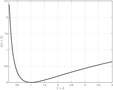
Figure 1: Bregman curve $\gamma$ in eq. 13.

Definition 2 (Bregman truncation).

Given an eigendecomposition $X=ZMZ^{*}\in\mathbb{H}^{n}$, $M=\operatorname{diag}(\mu_{1},\ldots,\mu_{n})$, construct the index set $\mathcal{I}_{X}^{\star}$ of cardinality $\#\mathcal{I}_{X}^{\star}=r<n$ by sorting the sequence $\{\gamma(\mu_{i})\}_{i=1}^{n}$ and selecting the indices corresponding to the largest values i.e.

$$\mathcal{I}_{X}^{\star}=\arg\max_{\begin{subarray}{c}\mathcal{I}\subset\{1,\ldots,n\}\\ \#\mathcal{I}=r\end{subarray}}\sum_{j\in\mathcal{I}}\gamma(1+\mu_{j}).$$ (14)

We define the Bregman truncation (BT) of $X$ to order $r$ by

$$\mathbb{H}^{n}\ni\mathopen{\hbox{\set@color${\langle}$}\mkern 2.0mu\kern-3.49998pt\leavevmode\hbox{\set@color${\langle}$}}X\mathclose{\hbox{\set@color${\rangle}$}\mkern 2.0mu\kern-3.49998pt\leavevmode\hbox{\set@color${\rangle}$}}_{r}=Z^{\star}M^{\star}(Z^{\star})^{*},$$ (15)

where the columns $Z^{\star}\in\mathbb{C}^{n\times r}$ (resp. $M^{\star}\in\mathbb{C}^{r\times r}$) are constructed from $Z$ (resp. $M$) by deleting column $j$ if $j\not\in\mathcal{I}_{X}^{\star}$. Similarly, the diagonal matrix $M^{\star}\in\mathbb{C}^{r\times r}$ is constructed from $M$ by deleting row $j$ and column $j$ if $j\not\in\mathcal{I}_{X}^{\star}$.

As we will show in Theorem 1, eq. 15 in Definition 2 is a minimiser of the optimisation problem (10).

Corollary 1.

When $B\in{\mathbb{H}^{n}_{+}}$, $\mathopen{\hbox{\set@color${\langle}$}\mkern 2.0mu\kern-3.49998pt\leavevmode\hbox{\set@color${\langle}$}}B\mathclose{\hbox{\set@color${\rangle}$}\mkern 2.0mu\kern-3.49998pt\leavevmode\hbox{\set@color${\rangle}$}}_{r}=\llbracket B\rrbracket_{r}$.

Proof.

If $B\in{\mathbb{H}^{n}_{+}}$ the eigenvalues of $I+G$ will be bounded from below by $1$ and since $\gamma$ is an increasing function on $[1,\infty)$ the index set $\mathcal{I}_{G}^{\star}$ constructed in eq. 14 selects the same $r$ principal directions as a TSVD. ∎

Before presenting our main result we first look at an example using a diagonal matrix to develop some intuition.

Example 1 (Diagonal matrix $S$).

Let us consider a concrete example of this approximation where $n=10$, $r=5$ and $S=I+G$ is diagonal matrix, where

$$G=\operatorname{diag}(\underbracket{-0.4699}_{\textbf{\color[rgb]{0,1,1}{\emph{BT}}}},\underbracket{-0.3530}_{\textbf{\color[rgb]{0,1,1}{\emph{BT}}}},-0.3097,0.1988,0.2211,\overbracket{0.5057}^{\textbf{\color[rgb]{1,0.37,1}{\emph{TSVD}}}},\overbracket{0.5479}^{\textbf{\color[rgb]{1,0.37,1}{\emph{TSVD}}}},\overbracket{\underbracket{0.7295}_{\textbf{\color[rgb]{0,1,1}{\emph{BT}}}}}^{\textbf{\color[rgb]{1,0.37,1}{\emph{TSVD}}}},\overbracket{\underbracket{0.7684}_{\textbf{\color[rgb]{0,1,1}{\emph{BT}}}}}^{\textbf{\color[rgb]{1,0.37,1}{\emph{TSVD}}}},\overbracket{\underbracket{1.0}_{\textbf{\color[rgb]{0,1,1}{\emph{BT}}}}}^{\textbf{\color[rgb]{1,0.37,1}{\emph{TSVD}}}}).$$

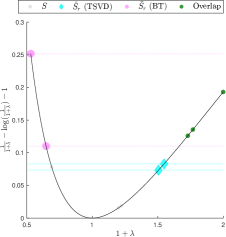
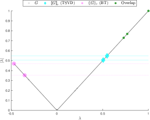
Figure 2: This depicts the situation in Example 1 where we compare a TSVD and Bregman truncations of a diagonal matrix $I+G$. The continuous curve traced on the left is eq. 13.

The brackets indicate which eigenvalues are selected by the rank $r$ TSVD and the Bregman truncation to the same order. Figure 2 shows how the two truncations differ. In the left figure, we show the image of these values under $x\mapsto\gamma(1+x)$, whereas in the right we show them under that of $x\mapsto|x|$. It is clear that selecting the two negative eigenvalues leads to a smaller objective value for $\gamma$ than those selected by a TSVD. The Bregman truncation selects "principal directions" according to the curve defined in (13). Furthermore,

$$0.2685=\mathcal{D}_{\textnormal{LD}}(I+\mathopen{\hbox{\set@color${\langle}$}\mkern 2.0mu\kern-3.49998pt\leavevmode\hbox{\set@color${\langle}$}}G\mathclose{\hbox{\set@color${\rangle}$}\mkern 2.0mu\kern-3.49998pt\leavevmode\hbox{\set@color${\rangle}$}}_{r},I+G)<\mathcal{D}_{\textnormal{LD}}(I+\llbracket G\rrbracket_{r},I+G)=0.4741.$$

Returning to the general case of preconditioning eq. 1, we now prove the following result.

Theorem 1.

Let $S=Q(I+G)Q^{*}$ be as in eq. 2. Then the preconditioner of $S$ defined by

$${\overline{S}_{r}}=Q(I+\mathopen{\hbox{\set@color${\langle}$}\mkern 2.0mu\kern-3.49998pt\leavevmode\hbox{\set@color${\langle}$}}G\mathclose{\hbox{\set@color${\rangle}$}\mkern 2.0mu\kern-3.49998pt\leavevmode\hbox{\set@color${\rangle}$}}_{r})Q^{*}$$ (16)

is a minimiser of the following problem:

$$\operatorname*{minimise}_{P\in{\mathbb{H}^{n}_{++}}}\quad \mathcal{D}_{\textnormal{LD}}(P,S)$$ (17a)

$$\operatorname*{s.t.}\quad P=Q(I+W)Q^{*},$$ (17b)

$$W\in\mathbb{H}^{n},$$ (17c)

$$\operatorname{rank}(W)\leq r.$$ (17d)

Furthermore, $n-r$ eigenvalues of ${\overline{S}_{r}}^{-1}S$ are given by $1+\lambda_{i}(G)$, $i\in\{1,\ldots,n\}\setminus\mathcal{I}_{G}^{\star}$, where $\mathcal{I}_{G}^{\star}$ is the index set given by eq. 14. The remaining $r$ eigenvalues equal $1$.

Proof.

Since the $\mathcal{D}_{\textnormal{LD}}$ is invariant to congruence transformations,

$$\mathcal{D}_{\textnormal{LD}}(P,S)=\mathcal{D}_{\textnormal{LD}}(I+W,I+G),$$

where $G=Q^{-1}BQ^{-*}$. We derive a lower bound for $W\mapsto\mathcal{D}_{\textnormal{LD}}(I+W,I+G)$ for matrices $W$ on the form eq. 17b. Recall from eq. 7 that we have

$$I+W=I+U\Lambda U^{*},$$

$$I+G=I+V\Theta V^{*}l$$

Note that only $r$ values of $\lambda$ are nonzero. Using the bound from [9] we have

$$\operatorname{trace}\big{(}PS^{-1}\big{)}\geq\sum_{i=1}^{n}\frac{1+\lambda_{i}}{1+\theta_{i}}.$$

Note that

$$-\log\det(PS^{-1})=-\sum_{i=1}^{n}\log\left(\frac{1+\lambda_{i}}{1+\theta_{i}}\right).$$

It is easy to see that

$$\mathcal{D}_{\textnormal{LD}}(P,S)\geq\sum_{i\not\in\{1,\ldots,n\}\setminus\mathcal{I}_{G}^{\star}}\Big{(}\frac{1+\lambda_{i}}{1+\theta_{i}}-\log\left(\frac{1+\lambda_{i}}{1+\theta_{i}}\right)-1\Big{)},$$

and this lower bound is attained by the choice $W=\mathopen{\hbox{\set@color${\langle}$}\mkern 2.0mu\kern-3.49998pt\leavevmode\hbox{\set@color${\langle}$}}G\mathclose{\hbox{\set@color${\rangle}$}\mkern 2.0mu\kern-3.49998pt\leavevmode\hbox{\set@color${\rangle}$}}_{r}$ in eq. 17b. ∎

Corollary 2.

When $B\in{\mathbb{H}^{n}_{+}}$, ${\overline{S}_{r}}=\widehat{S}_{r}$, where $\widehat{S}_{r}$ is the preconditioner proposed in [6].

Finally, the following result tells us when we can expect the Bregman truncation to be exact:

Corollary 3.

The Bregman truncation is exact if $\operatorname{rank}(B)\leq r$.

While Corollary 3 is trivial, the result highlights two interesting aspects of designing a preconditioner for $S$ within the framework presented in this paper. First, while the rank of $B$ may be much greater than $r$, the numerical rank of $G$ may be small, in particular when $A$ is ill-conditioned [18]. This suggests that a modest target rank $r$ could be sufficient to capture the principal information of the error. We investigate this numerically in Section 4. Secondly, suppose we choose a sparse matrix $A$ such that $A\approx S$ (in some sense) whose factors we can compute within some computational budget and, ideally, with limited fill. In the implementation of a Cholesky procedure, a fill-reducing algorithm can be used as part of the factorisation of a matrix $A$. In this case the factors are typically given up to a permutation matrix $P$:

$$CC^{*}=PAP^{\top},$$

so $A=QQ^{*}=P^{-1}CC^{*}P^{-*}$. In addition, any permutation matrix will also have an effect on the term $G=Q^{-1}BQ^{-*}$ to which we seek a low rank approximation. Indeed, recall $B=S-A$ and note that rank is not well-behaved under addition in the sense that for two Hermitian full rank matrices:

$$0\leq\operatorname{rank}(S-A)=\operatorname{rank}(B)\leq n.$$

It is therefore interesting to consider strategies whereby the permutation matrix $P$ is selected such that the rank of $B$ is as close to $r$ as possible. In other words we therefore have two objectives: choose a factor $Q=P^{-1}C$ with a suitable structure or size (e.g. sparsity) whilst minimising the numerical rank of $B$. We return to this in Section 5.

2.2 Unknown approximation basis

It is instructive to look at the case where we have fixed an approximation basis $U$ for $W$ for which $U\neq V$ and we must determine the $r$ eigenvalues of $W$ that provide the best approximation in the Bregman log determinant divergence. Keeping in mind that $V$ is fixed, we define the following function to ease notation:

$$\psi(\lambda_{i})=\sum_{j=1}^{n}(v_{i}^{*}u_{j})^{2}\Big{(}\frac{1+\lambda_{i}}{1+\theta_{j}}-\log\big{(}\frac{1+\lambda_{i}}{1+\theta_{j}}\big{)}-1\Big{)}.$$

That means solving the following problem with $\Lambda$ as variable:

$$\operatorname*{minimise}_{\Lambda=\operatorname{diag}(\lambda_{1},\ldots,\lambda_{n})}\quad \sum_{i=1}^{n}\psi(\lambda_{i})$$ (18a)

$$\operatorname*{s.t.}\quad \operatorname{rank}(\Lambda)\leq r.$$ (18b)

Note that $\operatorname{dom}\log=\mathbb{R}^{n}_{++}$ implies $\lambda_{i}\in(-1,\infty)$, $i=1,\ldots,n$. From the optimality conditions we see that eq. 18 is minimised when, for some indices $\mathcal{R}^{\star}\subset\{1,\ldots,n\}$, $\#\mathcal{R}^{\star}=r$ we have

$$\psi^{\prime}(\lambda_{i})=\sum_{j=1}^{n}(u_{i}^{*}v_{j})^{2}\Big{(}\frac{1}{1+\theta_{j}}-\frac{1}{1+\lambda_{i}^{\star}}\Big{)}=0,\quad i\in\mathcal{R}^{\star}.$$

Using $T_{ij}=(u_{i}^{*}v_{j})^{2}$ and simplifying we get

$$\sum_{j=1}^{n}\frac{T_{ij}}{1+\theta_{j}}=\sum_{j=1}^{n}\frac{T_{ij}}{1+\lambda_{i}^{\star}}=\frac{1}{1+\lambda_{i}^{\star}}\sum_{j=1}^{n}T_{ij}=\frac{1}{1+\lambda_{i}^{\star}}.$$

It can now be seen that $\frac{1}{1+\lambda_{i}^{\star}}$ is a convex combination of $\frac{1}{1+\theta_{j}}$, $j=1,\ldots,n$ by rearranging the expression above:

$$\lambda_{i}^{\star}=\frac{1}{\sum_{j=1}^{n}\frac{T_{ij}}{1+\theta_{j}}}-1,\quad i=1,\ldots,n.$$ (19)

Eq. 19 therefore provides an explicit characterisation of a solution to (18) and $1+\lambda_{i}^{\star}$ is proportional to a weighted harmonic mean of $1+\theta_{j}$, $j=1,\ldots,n$. In order to determine the set of indices $\mathcal{R}^{\star}$, problem (18) can, similarly to what was done in Section 2.1, be formulated as a combinatorial problem:

$$\min_{d\in\{0,1\}^{n}}\quad \sum_{i=1}^{n}\big{(}\psi(0)-\psi(\lambda_{i}^{\star})\big{)}(1-d_{i})$$ (20a)

$$\operatorname*{s.t.}\quad \sum_{i=1}^{n}d_{i}=r.$$ (20b)

The first factor in the sum represents the improvement to the objective by including $\lambda_{i}^{\star}$ in the Bregman truncation. Problem (20) may not be practical to solve in practice as it requires the evaluation of the bistochastic matrix $T$. We investigate this problem further in a sequel and in this paper only pursue the case where $U=V$ as in Section 2.1.

3 Determining the leading Bregman directions

In the context of low-rank matrix approximations the tacit assumption is often that the objective is to find its dominant directions with respect to the $\ell_{2}$ and Frobenius norms thanks to the Young-Eckhart-Mirksy theorem [13]. By Corollary 1 we know that the leading Bregman directions do not always correspond to those of a TSVD, so we cannot readily apply the popular matrix approximation methods such as the randomised SVD and Nyström approximations from randomised linear algebra [17]. Solutions to the rangefinder problem [25] produce matrices $O\in\mathbb{R}^{n\times r}$ with orthonormal columns used to approximate a given matrix $Z$ such that

$$Z\approx OO^{*}ZOO^{*}.$$

This approximation comes at a cost of $O(nr^{2})$ which greatly improves on the naïve $O(n^{3})$ cost of constructing $\llbracket Z\rrbracket_{r}$. $O$ is typically constructed via sketching where the columns of $O$ are constructed from a reduced (or "thin") QR decomposition of a Gaussian matrix $\Omega\in\mathbb{R}^{n\times r}$, leading to the randomised SVD. We also mention the Nyström approximation [14, 29]

$$Z\approx Z\Omega(\Omega^{*}Z\Omega)^{+}(Z\Omega)^{*}$$

which is valid when $Z\in{\mathbb{H}^{n}_{+}}$ and can be shown is a range-restricted matrix approximation that is optimal in the Bregman divergence [6]. Note that modifications can be made to the Nyström approximation in order to produce a numerically stable procedure for indefinite $Z$ [26]. These methods are economical approximations of a TSVD, and do not a priori provide an approximate Bregman truncation without some modification. The subject of this section is therefore to develop a scheme allowing us to approximate the preconditioner ${\overline{S}_{r}}$ defined in eq. 16 when we only have access to the action of $S$ on vectors.

We present a conceptual iterative scheme in Algorithm 1 to determine the leading Bregman directions (cf. Definition 2) that comprise $\mathopen{\hbox{\set@color${\langle}$}\mkern 2.0mu\kern-3.49998pt\leavevmode\hbox{\set@color${\langle}$}}G\mathclose{\hbox{\set@color${\rangle}$}\mkern 2.0mu\kern-3.49998pt\leavevmode\hbox{\set@color${\rangle}$}}_{r}$ for a given matrix $G$. This algorithm starts by computing the two extremal eigenvalues of a matrix and then, based on which of these attains the maximum value under the image of $\gamma$ (cf. eq. 13), iteratively computes the next candidate on this curve. Pictorially, this algorithm approaches the abscissa at $\lambda=0$ in Figure 2 from the left and the right. We shall use the pseudocode compute_eigenpair_largest and compute_eigenpair_smallest to refer to procedures that compute (or approximate) the eigenpair corresponding to the largest and smallest eigenvalue of an input matrix, with the Lanczos procedure [15] being a suitable choice. To ease the notation, we shall not differentiate between computing exact and approximate eigenvalues, although in practice we compute with the latter. By deflating existing directions in line 9, Algorithm 1 computes only the extremal eigenvalues resulting in only $r+1$ iterations of e.g. Lanczos in total. Suppose $d$ is the average number of nonzero elements in a row of the target matrix, then the computational cost of Algorithm 1 is $O(dn^{2})$. As a result, Algorithm 1 is $O(dn^{2}r)$.

Naïve implementations of Lanczos are susceptible round-off errors, which affects numerical stability. For sparse matrices, the Lanczos procedure can be very rapid so it may therefore be more efficient or economical to compute the $2r$ extremal eigenvalues using library implementations of Lanczos ($r$ largest and $r$ smallest). If a rank $r$ truncation is desired, the eigenvalues can then be sorted using the curve in (13) produce a Bregman truncation. In similar vein, it may be advantageous to use the modified Nyström approximation of [26] to produce the $2r$ extremal eigenvalues of a target matrix as opposed to Algorithm 1.

Algorithm 1 Conceptual Bregman–Lanczos iteration scheme

1:Indefinite matrix $G\in\mathbb{H}^{n}$, truncation rank $r<n$.

2:Bregman truncation $\mathopen{\hbox{\set@color${\langle}$}\mkern 2.0mu\kern-3.49998pt\leavevmode\hbox{\set@color${\langle}$}}G\mathclose{\hbox{\set@color${\rangle}$}\mkern 2.0mu\kern-3.49998pt\leavevmode\hbox{\set@color${\rangle}$}}_{r}$ of the matrix $G$.

3:$(v^{\oplus},\lambda^{\oplus})\leftarrow$ compute_eigenpair_largest $(G)$

4:$(v^{\ominus},\lambda^{\ominus})\leftarrow$ compute_eigenpair_smallest $(G)$

5:if $\gamma(\lambda^{\ominus})<\gamma(\lambda^{\oplus})$ then $\triangleright$ $\gamma$ is defined in eq. 13

6:     $(v_{1},\lambda_{1})\leftarrow(v^{\oplus},\lambda^{\oplus})$

7:else

8:     $(v_{1},\lambda_{1})\leftarrow(v^{\ominus},\lambda^{\ominus})$

9:end if

10:for $i=2,\ldots,r$ do

11:     $G_{\text{defl.}}\leftarrow G-\sum_{j=1}^{i}\lambda_{j}v_{j}v_{j}^{*}$ $\triangleright$ Deflate existing directions

12:     if $\operatorname{sign}(\lambda_{i-1})>0$ then $\triangleright$ Approach $\gamma$ from the left or right? See left panel of Figure 2

13:         $(v^{\oplus},\lambda^{\oplus})\leftarrow$ compute_eigenpair_largest $(G_{\text{defl.}})$

14:     else

15:         $(v^{\ominus},\lambda^{\ominus})\leftarrow$ compute_eigenpair_smallest $(G_{\text{defl.}})$

16:     end if

17:     if $\gamma(\lambda^{\ominus})<\gamma(\lambda^{\oplus})$ then $\triangleright$ Choose between the two candidate directions based on $\gamma$ values.

18:         $(v_{i},\lambda_{i})\leftarrow(v^{\oplus},\lambda^{\oplus})$

19:     else

20:         $(v_{i},\lambda_{i})\leftarrow(v^{\ominus},\lambda^{\ominus})$

21:     end if

22:end for

23:$\mathopen{\hbox{\set@color${\langle}$}\mkern 2.0mu\kern-3.49998pt\leavevmode\hbox{\set@color${\langle}$}}G\mathclose{\hbox{\set@color${\rangle}$}\mkern 2.0mu\kern-3.49998pt\leavevmode\hbox{\set@color${\rangle}$}}_{r}\leftarrow\sum_{j=1}^{r}\lambda_{j}v_{j}v_{j}^{*}$

Algorithm 1 uses the function $\gamma$ to select the eigenvalues of the Bregman truncation, which is specific to the Bregman log determinant divergence. In a future work, we aim to investigate truncations stemming from other divergences.

4 Applications to the preconditioned conjugate gradient method

We now demonstrate the convergence of PCG using the preconditioner ${\overline{S}_{r}}$ defined in eq. 16. First we recall the following result from [16].

Theorem 2.

Let $S\in{\mathbb{H}^{n}_{++}}$ and $x_{0}\in\mathbb{C}^{n}$ be an initial guess for the solution of the system $Sx=b$ for some $b\in\mathbb{C}^{n}$. Further, let $\mathcal{M}$ denote the inverse of a preconditioner. The $k$^th iterate of PCG, $x_{k}$, satisfies:

$$\|x-x_{k}\|_{S} =\inf_{\begin{subarray}{c}p_{k}\in\mathcal{P}_{k}\\ p_{k}(0)=1\end{subarray}}\|p_{k}(\mathcal{M}S)(x-x_{0})\|_{S},$$

$$\|x-x_{k}\|_{S} \leq\inf_{\begin{subarray}{c}p_{k}\in\mathcal{P}_{k}\\ p_{k}(0)=1\end{subarray}}\sup_{z\in\lambda(\mathcal{M}S)}|p_{k}(z)|\|x-x_{0}\|_{S},$$

$$\|x-x_{k}\|_{S} \leq 2\Big{(}\frac{\sqrt{\kappa_{2}(\mathcal{M}S)}-1}{\sqrt{\kappa_{2}(\mathcal{M}S)}+1}\Big{)}^{k}\|x-x_{0}\|_{S},$$ (21)

where $\mathcal{P}_{k}$ is the space of polynomials of order at most $k$.

The following is a generalisation of a result in [6].

Corollary 4.

Let $\mu_{i}$, $i\in\{1,\ldots,n\}\setminus\mathcal{I}_{G}^{\star}$ denote the eigenvalues of ${\overline{S}_{r}}^{-1}S$. Using ${\overline{S}_{r}}$ as a preconditioner to solve (1) using PCG for some initial guess $x_{0}$, we have

$$\|x-x_{k}\|_{S}\leq\inf_{\begin{subarray}{c}p_{k}\in\mathcal{P}_{k}\\ p_{k}(0)=1\end{subarray}}\sup_{i\in\{1,\ldots,n\}\setminus\mathcal{I}_{G}^{\star}}|p_{k}(\mu_{i})|\|x-x_{0}\|_{S}.$$ (22a)

Further, PCG will converge in at most $\operatorname{rank}(B)-r+1$ steps [15, Theorem 10.2.5].

When $B\in{\mathbb{H}^{n}_{+}}$, Corollary 1 informs us that the Bregman truncation coincides with the TSVD. If also $\operatorname{rank}(B)<n$, [6, Theorem 2] states that the preconditioner minimises the $\ell_{2}$ condition number of the preconditioned matrix. Such a result does note hold when $B$ is indefinite, although the significance of this is not clear. The condition number is often used as a metric for evaluating the fitness of preconditioners thanks to its presences in the (pessimistic) upper bound eq. 21. In Section 4, we provide evidence that the Bregman truncation is able to capture more meaningful information from the "error matrix" $G$ which appears to improve the convergence PCG.

The rest of this section is organised as follows. First, we present an example using synthetic data in Section 4.1 to further develop the intuition from Example 1. Section 4.2 explores how to use the framework presented above to improve on the standard incomplete Cholesky preconditioners using a low-rank compensation representing the leading Bregman directions of the factorisation error. Section 4.3 explores an application of the framework presented above to interior point methods for linear programmes. Here we will only consider matrices that do not admit incomplete Cholesky factors and present an algorithm which uses dynamic regularisation to achieve an approximate incomplete Cholesky factorisation $A=QQ^{*}$. The resulting preconditioner ${\overline{S}_{r}}$ defined in eq. 16 is then compared to several alternatives.

4.1 Synthetic data

Recall Figure 2, which presented a simple example using diagonal matrices, and showed how the Bregman truncation differs from a TSVD. To further develop the intuition, we now consider a problem instance using dense matrices with an application to PCG.

We construct $S=A+B$ by selecting two randomly generated dense matrices $A\in{\mathbb{H}^{n}_{++}}$ and $B\in\mathbb{H}^{n}$ for $n=50$ in the following way. Letting $A=Z\Lambda Z^{*}$ denote an eigendecomposition of $A$, we have $S=Z(\Lambda+Z^{*}BZ)Z^{*}$. Since the Bregman divergence is invariant to orthogonal transformations, we use the canonical basis for $Z$ and randomly generate a positive diagonal matrix $A=\Lambda$ by sampling the Gaussian distribution and taking the absolute value to ensure positive definiteness. We randomly generate an orthogonal basis for $B$ and sample its eigenvalues from the Gaussian distribution, scaling them in such a way to ensure $S$ is positive definite (note $B$ remains indefinite in this way). We then construct the preconditioners $\widehat{S}_{r}$ and ${\overline{S}_{r}}$ given in eq. 6 and eq. 16, respectively, for the instances of $A$ and $B$ given above using rank $r=10$. For a random $b\in\mathbb{R}^{n}$, we solve $Sx=b$ using PCG where we use:

1. no preconditioner,

2. symmetric preconditioning using the zero fill incomplete Cholesky factors $Q$ described above,

3. left-preconditioning using $\widehat{S}_{r}=Q(I+\llbracket G\rrbracket_{r})Q^{*}$ (eq. 6),

4. and left-preconditioning using ${\overline{S}_{r}}=Q(I+\mathopen{\hbox{\set@color${\langle}$}\mkern 2.0mu\kern-3.49998pt\leavevmode\hbox{\set@color${\langle}$}}G\mathclose{\hbox{\set@color${\rangle}$}\mkern 2.0mu\kern-3.49998pt\leavevmode\hbox{\set@color${\rangle}$}}_{r})Q^{*}$ (eq. 16).

The results are shown in Figure 3; the bottom left panel shows the eigenvalues of matrices in this experiment. The top two panels show the eigenvalues of the two truncations we consider in this paper (note that we now plot the image of $\gamma$ in a semilogarithmic plot in order to clearly distinguish between the different eigenvalues). While the two truncations share some choices of eigenvalues, we clearly see that they fundamentally select according to different criteria. We also compare the two preconditioners based on these truncations as well as the symmetric preconditioner using the factors of $A$ in terms of PCG convergence. While both preconditioners perform better than simply preconditioning with $A$, we conclude that the Bregman truncation leads to superior performance (i.e., fewer iterations of PCG required). In the next section, we look at less contrived numerical examples to further support our theoretical findings above.

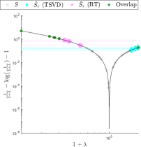
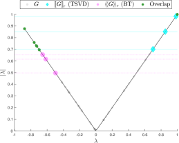
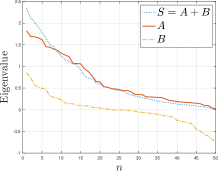
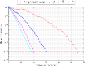
Figure 3: Comparison of eigenvalues selected by the Bregman truncation and TSVD, where $n=50$ and $r=10$. Note that the top left plot is semilogarithmic.

4.2 Improving incomplete Cholesky using low-rank compensation

We select real symmetric positive definite matrices from the SuiteSparse Matrix Collection [21] of varying size $n$ and use three values of $r$ relative to $n$:

$$r=\lfloor n\times c\rfloor,\quad c\in\{0.01,0.05,0.1\}$$ (23)

In this section, we let $QQ^{*}=A\approx S$ be given as a zero fill incomplete Cholesky factorisation of a target matrix $S$, and we let $B=S-A$ denote the symmetric and possibly indefinite approximate factorisation error. Using the same four preconditioners described in Section 4.1 and the three choices of rank in eq. 23, Section 4.2 shows the condition number, Bregman divergence and the number of PCG iterations at termination, which either occurs if the relative residual is below the tolerance $10^{-10}$ or after 100 iterations. The entries "-" in the table correspond to instances where the tolerance was not reached either due to PCG stagnating or the maximum number of iterations was reached. From Section 4.2 we note that preconditioning is essential even for the moderately sized problems since the unpreconditioned CG fails to converge. There are also some cases where convergence is not obtained even with symmetric preconditioning using incomplete Cholesky. However, the table shows that the compensation using a low-rank matrix can be extremely beneficial for convergence. We also observe that the preconditioner that yields the smallest $\ell_{2}$ condition number is not always the one for which PCG converges in the fewest number of steps.

We observe a few trends for the two preconditioners $\widehat{S}_{r}$ and ${\overline{S}_{r}}$. Importantly, we observe that PCG almost always requires more iterations when using $\widehat{S}_{r}$, which is based on a TSVD, than ${\overline{S}_{r}}$, based on a BT. In many of the cases, PCG with the latter requires significantly fewer iterations, which is well-aligned with our intuition that the Bregman log determinant divergence is a useful measure of the quality of a preconditioner. The numerical values of the Bregman divergence between the preconditioners and the target matrix $S$ (i.e. $\mathcal{D}_{\textnormal{LD}}(\mathcal{P},S)$ for different definitions of $\mathcal{P}$) are aligned with Theorem 1. As expected, increasing the rank results in fewer iterations for convergence required by both preconditioners. For some problem instances we also see that the difference between $\widehat{S}_{r}$ and ${\overline{S}_{r}}$ becomes smaller (both in terms of PCG iterations required and the residual) as the rank $r$ increases. We now take a closer look at select instances from Section 4.2 to explain these phenomena.

Table 1: Results for 10 matrices selected from the SuiteSparse Matrix Collection. The residual tolerance was set to $10^{-10}$. For each row, we have highlighted the smallest number across the relevant columns.

Problem instance

$n$

$r$

Iteration count

$\ell_{2}$ condition number

Bregman divergence

No PC

$A$

$\widehat{S}_{r}$

${\overline{S}_{r}}$

No PC

$A$

$\widehat{S}_{r}$

${\overline{S}_{r}}$

$A$

$\widehat{S}_{r}$

${\overline{S}_{r}}$

[ head to column names, ]icholresults_tex.csvName=%\DeclareUrlCommand\UScore{\urlstyle{rm}}\Name

o

First we look at problem instances where the two preconditioners $\widehat{S}_{r}$ and ${\overline{S}_{r}}$ appear to yield similar results. From Section 4.2 we see that the two preconditioners perform similarly for HB/bcsstm07. In Section 4.2 we look at the row corresponding to $r=21$ and inspect the eigenvalues of the target matrix $S$ and its constituents $A$ and $B$ as well as the Bregman and SVD curves for the two preconditioners. We also show the convergence of PCG. Although there is some overlap in the eigenvalues selected by the two truncations we see that there are also some differences. However, due to the spectrum of the target matrix the two choices contribute more or less equally to the Bregman divergence, which is also clear from Section 4.2. Changing $r$ does not result in large deviations between the two preconditioners, so this example illustrates that while Corollary 1 does not apply here, the two truncations have enough similarities to result in similar PCG performance.

Figure 4: Experiment with HB/bcsstm07 ($n=420$ and $r=21$). Top: SVD and Bregman curve. Bottom: eigenvalues and PCG performance. Note that the top left plot is semilogarithmic.

Next we look at HB/1138_bus where ${\overline{S}_{r}}$ greatly outperforms $\widehat{S}_{r}$. Indeed, we see that PCG using the latter fails to reach the desired tolerance. This is explained in Section 4.2, where we see that the spectrum of $G$ is such that the two truncations select different eigenvalues resulting in different PCG behaviour. We affirm that selecting leading principal directions using the magnitude of the singular values is not necessarily always well-suited when constructing preconditioners of the form considered here. This supports our reasoning that $\gamma$ provides a more useful measure than the absolute value. We emphasise that the truncations agree on 9 out of 11 directions, and we see little difference in terms of magnitude of the selected eigenvalues, but a much a larger difference on the Bregman curve. This leads to a noticable improvement in PCG convergence using the Bregman truncation preconditioner despite differing by only two principal directions. As the rank of the low-rank approximation increases, the advantage of the ${\overline{S}_{r}}$ remains in this case. In general, the differences between the two preconditioners depends on the spectrum and numerical rank of the matrix $G$.

Figure 5: Experiment with HB/1138_bus ($n=1138$ and $r=11$). Top: SVD and Bregman curve. Bottom: eigenvalues and PCG performance. Note that the top left plot is semilogarithmic.

Finally, we comment on another example from Section 4.2, namely HB/bcsstk22. This problem demonstrates how the selection of eigenvalues can affect PCG performance, this time using a symmetric stiffness matrix stemming from a structural problem. In Section 4.2, we see from the Bregman curve that we may (based on the previous numerical evidence) expect faster PCG convergence preconditioning using ${\overline{S}_{r}}$ over $\widehat{S}_{r}$, despite only selecting two principal directions. Here, the two truncations select different eigenvalues, and the top two panels show how the Bregman and SVD curves value these directions quite differently. However, using ${\overline{S}_{r}}$, we observe slightly faster PCG convergence.

Figure 6: Experiment with HB/bcsstk22 ($n=138$ and $r=2$). Top: SVD and Bregman curve. Bottom: eigenvalues and PCG performance. Note that the top left plot is semilogarithmic.

Overall the magnitude of eigenvalues simply does not capture the desired nearness we want between a matrix and its preconditioner. We clearly see that the Bregman divergence is a more suitable tool to evaluate preconditioners and that this form provides a nearness measure that better captures the desiderata of a preconditioned matrix. While the matrices considered here are relatively small, our methodology scales to the large-scale setting by the nature of Algorithm 1. In this case, the indefiniteness of the term $B$ may not be known, and it may even be difficult to assess to what extent the two preconditioners ${\overline{S}_{r}}$ and $\widehat{S}_{r}$ compare. However, it is particularly interesting that even for small differences in absolute value between the eigenvalues chosen between ${\overline{S}_{r}}$ and $\widehat{S}_{r}$, we see a pronounced effect on PCG convergence (cf. Section 4.2). Regardless of the type of truncation we use, a low rank compensation term can be very beneficial when used in conjunction with the incomplete Cholesky preconditioner as it (sometimes vastly) improves performance in both cases. We emphasise that the difference between the two preconditioners can vanish as $r$ increases. However, in large-scale applications, $r$ may be relatively small compared to $n$. It may therefore be very beneficial to consider ${\overline{S}_{r}}$ as it appears to capture more useful directions for this particular application depending on the spectrum of the target matrix.

4.3 Preconditioned interior point methods

Next we showcase the proposed preconditioner ${\overline{S}_{r}}$ using problems where the matrix in question does not admit an incomplete Cholesky factorisation. We present a robust incomplete Cholesky procedure which is guaranteed to produce suitable factors $Q$ and based on these propose a preconditioner of the form eq. 16.

In this section, we consider equality constrained minimisation where $f:\mathbb{R}^{n}\rightarrow\mathbb{R}$, $F:\mathbb{R}^{m\times n}$ and $b\in\mathbb{R}^{m}$:

$$\operatorname*{minimise}_{x\in\mathbb{R}^{n}}\quad f(x)$$ (24a)

$$\operatorname*{s.t.}\quad Fx=b,$$ (24b)

$$x\geq 0.$$ (24c)

The so-called Karush-Kuhn-Tucker (KKT) conditions are:

$$\nabla f(x^{\star})+F^{*}\nu=0,$$ (25a)

$$\phantom{\nabla f(x^{\star})+}\;\,Fx^{\star}=b.$$ (25b)

A Newton method for the updates $\Delta x$ and $\Delta\nu$ requires the solution of the following system:

$$\begin{bmatrix}\nabla^{2}f(x)&F^{*}\\ F&0\end{bmatrix}\begin{bmatrix}\Delta x\\ \Delta\nu\end{bmatrix}=\begin{bmatrix}-\nabla f(x)-A^{*}\nu\\ b-Fx\end{bmatrix}.$$ (26)

We often seek a solution $x^{\star}$ in the nonnegative orthant. An interior point method [27] replaces the constraint eq. 24c by adding the following logarithmic barrier function to an objective function for some $\mu>0$:

$$-\mu\sum_{i=1}^{n}\log(x_{i}),$$

since this discourages the variable $x$ from approaching zero. We restrict our attention to linear barrier subproblems so the objective function $f$ is, for some $c\in\mathbb{R}^{n}$, given by:

$$f(x)=c^{\top}x-\mu\sum_{i=1}^{n}\log(x_{i}).$$

The Hessian of $f$ at $x$ is the diagonal matrix defined by

$$\nabla^{2}f(x)=\mu\operatorname{diag}(x^{-2}).$$

By elimination of $\Delta x$ in eq. 26 we obtain the following Schur complement system:

$$S\Delta\nu=-F\nabla^{2}f(x)^{-1}\nabla f(x),\quad\text{where}\;\,S=F\nabla^{2}f(x)^{-1}F^{*}.$$ (27)

Note that $\nabla^{2}f(x)^{-1}$ degenerates as an interior point method iterates [22, Proposition 2.1] leading to ill-conditioning of eq. 27. Preconditioning is therefore important for the performance of indirect methods for interior point methods.

In the previous section we described a way to account for the factorisation error between a target matrix and its incomplete Cholesky factorisation by introducing a low-rank compensation term. In this section we look at instances of matrices $S$ in eq. 27 which do not a priori admit such a factorisation. Indeed, the standard incomplete Cholesky procedure can fail due to nonpositive pivots even for Hermitian positive definite matrices. Since diagonally dominant matrices always admit an incomplete Cholesky factorisation [32] one may replace the input matrix $S$ by

$$S+\alpha\operatorname{diag}(S_{11},\ldots,S_{nn}),$$ (28)

where $\alpha>0$ is a sufficiently large value that can depend on $S$ [24]. This modification adds a full rank term to the target matrix. This means modifying all diagonal elements of $S$ including the positive pivots. Alternatively, as presented in Algorithm 2, we may take a dynamic approach and only replace the nonpositive pivots rather than adding a full rank diagonal matrix. The offending pivots are replaced by

$$\alpha=\max_{i\in\{1,\ldots,n\}}\sum_{j=1}^{n}\frac{|S_{ij}|}{S_{ii}}.$$ (29)

This is a heuristic, and in general this value may have to be selected on a trial-and-error basis. We note that other robust approaches to computing incomplete Cholesky factorisations exist in the context of the conjugate gradient method, see [1, 19, 20, 34] and [32] for an overview. To illustrate the difference between the dynamic regularisation in Algorithm 2 and the modification in eq. 28 in the present context, suppose $H\in\mathbb{H}^{n}$ is a suitable matrix chosen such that the sum $S+H$ admits an incomplete Cholesky factorisation while $S$ does not i.e.

$$S+H=QQ^{*}.$$ (30)

We have

$$S=Q(I-Q^{-1}HQ^{-*})Q^{*}.$$

Recall that the definition of the Bregman preconditioner ${\overline{S}_{r}}$ in eq. 16 uses a low-rank truncation to the indefinite term $G=-Q^{-1}HQ^{-*}$. We observe that $G$ and $H$ have the same rank. It is thus advantageous to suppress the rank of $H$ so the low-rank information captured by $G$ represents the factorisation error given by the approximation $S\approx QQ^{*}$ rather than the (albeit necessary) regularisation $H$. We therefore propose a preconditioner for eq. 27 based on a robust incomplete Cholesky factorisation given by Algorithm 2 and introduce a low-rank approximation of the scaled error $G$. Again, we shall compare the TSVD to the Bregman truncation in Definition 2. Algorithm 3 summarises the steps needed to construct a Bregman preconditioner ${\overline{S}_{r}}$ based on finding a candidate factorisation of a target matrix $S$ using Algorithm 2. The TSVD-based preconditioner $\widehat{S}_{r}$ is obtained in a similar fashion. Note that we can carry out Algorithm 3 by simply making products with $S$ and triangular solves with $Q$.

Algorithm 2 In-place Robust Incomplete Cholesky Decomposition

1:Target matrix $S\in\mathbb{H}^{n}$, diagonal threshold diag_tol.

2:Matrix $S$ representing the robust incomplete Cholesky factor

3:Compute $\alpha$ from eq. 29

4:for $k=1$ to $n$ do

5:    if $S_{kk}<\texttt{diag\_tol}$ then

6:       $S_{kk}\leftarrow\alpha$ $\triangleright$ Regularise nonpositive pivots

7:    else

8:       $S_{kk}\leftarrow\sqrt{S_{kk}}$

9:    end if

10:    for $i=k+1$ to $n$ do

11:       if $S_{ik}\neq 0$ then

12:          $S_{ik}\leftarrow S_{ik}/S_{kk}$

13:       end if

14:    end for

15:    for $j=k+1$ to $n$ do

16:       for $i=j$ to $n$ do

17:          if $S_{ij}\neq 0$ then

18:             $S_{ij}\leftarrow S_{ij}-S_{ik}\cdot S_{jk}$

19:          end if

20:       end for

21:    end for

22:end for

23:for $i=1$ to $n$ do

24:    for $j=i+1$ to $n$ do

25:       $S_{ij}\leftarrow 0$

26:    end for

27:end for

Algorithm 3 Robust Incomplete Cholesky Preconditioner with Low-rank Error Compensation

1:Target matrix $S\in{\mathbb{H}^{n}_{++}}$, truncation rank $r<n$, diagonal threshold $\texttt{diag\_tol}>0$.

2:Preconditioner $Q(I+\mathopen{\hbox{\set@color${\langle}$}\mkern 2.0mu\kern-3.49998pt\leavevmode\hbox{\set@color${\langle}$}}G\mathclose{\hbox{\set@color${\rangle}$}\mkern 2.0mu\kern-3.49998pt\leavevmode\hbox{\set@color${\rangle}$}}_{r})Q^{\top}$

3:Obtain robust factor $Q$ by applying Algorithm 2 to $S$ with diagonal threshold diag_tol.

4:$G\leftarrow Q^{-1}SQ^{-\top}-I$

5:Apply Algorithm 1 to $G$ to obtain the $r$ principal Bregman pairs $(v_{i},\lambda_{i})$, $i=1,\ldots,r$.

6:$\mathopen{\hbox{\set@color${\langle}$}\mkern 2.0mu\kern-3.49998pt\leavevmode\hbox{\set@color${\langle}$}}G\mathclose{\hbox{\set@color${\rangle}$}\mkern 2.0mu\kern-3.49998pt\leavevmode\hbox{\set@color${\rangle}$}}_{r}\leftarrow\sum_{i=1}^{r}\lambda_{i}v_{i}v_{i}^{*}$.

We now describe our experimental setup and construction of matrices $S$ in eq. 27. We select matrices $F\in\mathbb{R}^{n\times m}$ based on linear programming problems from SuiteSparse and control the conditioning of the target matrix $S$ by constructing $D_{\tau}$ as the $m\times m$ diagonal matrix $m$ logarithmically spaces points between $10^{-\tau}$ and $10^{\tau}$:

$$D_{\tau}=\operatorname{diag}(10^{-\tau},\ldots,10^{\tau}).$$ (31)

For instance, $D_{0}=I$. There parameter $\tau$ therefore controls the condition number of

$$S:=FD_{\tau}^{-1}F^{*}.$$ (32)

We now provide numerical experiments where we solve

$$Sx=b$$

for random right-hand sides $b$ using the definition of $S$ in eq. 32. We study the performance of PCG in the following situations where $Q$ denotes the robust incomplete Cholesky factors $Q$ given by Algorithm 2:

1. No preconditioner.

2. Symmetric preconditioning using $Q$.

3. Symmetric preconditioning using the incomplete Cholesky factors $Q_{\alpha}$ given by

   $$Q_{\alpha}Q_{\alpha}^{\top}\approx S+\alpha\operatorname{diag}(S_{11},\ldots,S_{nn}),$$ (33)

   where $\alpha$ is computed from $S$ using eq. 29.

4. Left-preconditioning using the TSVD-based precondition $\widehat{S}_{r}$.

5. Left-preconditioning using ${\overline{S}_{r}}=Q(I+\mathopen{\hbox{\set@color${\langle}$}\mkern 2.0mu\kern-3.49998pt\leavevmode\hbox{\set@color${\langle}$}}G\mathclose{\hbox{\set@color${\rangle}$}\mkern 2.0mu\kern-3.49998pt\leavevmode\hbox{\set@color${\rangle}$}}_{r})Q^{*}$ given by Algorithm 3.

Section 4.3 shows the results where we have used different values of $r$ according to eq. 23 for the values $\tau\in\{0,1,2\}$. This allows us to study the various preconditioners and any interaction between the rank chosen and the conditioning of the target matrix $S$. In general, higher values of $\tau$ result in harder problems, and we see that there are some problems where PCG fails to converge for any of the preconditioners. We also see that larger values of $r$ result in fewer iterations required by PCG for both $\widehat{S}_{r}$ and ${\overline{S}_{r}}$. We observe that neither the unpreconditioned systems or those symmetrically preconditioned with $Q_{\alpha}$ converge to the desired tolerance of $10^{-7}$. Preconditioning with $Q$ only leads to convergence for relatively small $n$ when the target matrix is not too ill-conditioned. Overall, using a low-rank compensation term does in some cases lead to convergence depending on the chosen truncation. While preconditioning with $\widehat{S}_{r}$ based on a TSVD of $G$ leads to some instances of PCG convergence, we see that ${\overline{S}_{r}}$ leads to far superior results in general. In fact, there are instances where the spectrum of the matrix greatly affects how much of an improvement the preconditioner ${\overline{S}_{r}}$ is over $\widehat{S}_{r}$ (or the other alternatives).

In summary we have presented extensive numerical results for PCG applied to generally ill-conditioned matrices from interior point methods. We have compared results across four different preconditioners and stress-tested the proposed framework presented in this paper. The results indicate that the Bregman divergence is a suitable measure with which to compare a preconditioner against a target matrix. For completeness we also constructed the preconditioner

$$Q_{\alpha}(I+\mathopen{\hbox{\set@color${\langle}$}\mkern 2.0mu\kern-3.49998pt\leavevmode\hbox{\set@color${\langle}$}}G_{\alpha}\mathclose{\hbox{\set@color${\rangle}$}\mkern 2.0mu\kern-3.49998pt\leavevmode\hbox{\set@color${\rangle}$}}_{r})Q_{\alpha}^{*},$$

where

$$G_{\alpha}=Q_{\alpha}^{-1}SQ_{\alpha}^{-*}-I$$

but found that, just as with symmetric preconditioning with $Q_{\alpha}$, PCG failed to converge in all cases. The choice of factor to "extract" from the target matrix is therefore critical to the effectiveness of the proposed preconditioner.

Table 2: PCG results for KKT problems. The columns $Q_{\alpha}Q_{\alpha}^{*}$, $A$, TSVD and BT correspond to the preconditioner in eq. 33, the robust incomplete Cholesky preconditioner, $\widehat{S}_{r}$ and ${\overline{S}_{r}}$, respectively. The residual tolerance is $10^{-7}$. For each row, we have highlighted the smallest number across the relevant columns.

5 Summary & outlook

We have presented a framework based on the Bregman log determinant divergence to derive an approximation of a given matrix on the form of a Hermitian positive definite plus a low-rank approximation of an indefinite matrix. $Q$ is assumed to be known factors of a matrix $A$ that is in some sense close to $S$. The motivation for this work was to systematically account for factorisation errors $B=S-QQ^{*}$ when designing preconditioners for the iterative solution of linear systems eq. 1 involving the matrix $S$. In Section 2 we showed how the Bregman log determinant divergence generally leads to principal directions of a matrix that are different from a TSVD. This framework therefore allows us to choose an approximate factorisation $QQ^{*}\approx S$ (e.g. an incomplete Cholesky factorisation) and, depending on the computational budget, select a low-rank compensation term that captures the approximation error. We presented the proposed preconditioner eq. 16 based on this novel Bregman truncation and characterised a solution to the general problem where the basis for the truncation is unknown. In Section 3 we presented a conceptual iterative procedure for approximating these principal directions. Section 4 contained numerous numerical examples demonstrating the effectiveness of the approach over a similar TSVD-based preconditioner.

While the Bregman truncation provides a novel way of selecting a low-rank approximation, the results in Section 4.3 showed that the effectiveness of the proposed preconditioner heavily depends on the choice of facto $Q$ and how closely $QQ^{*}$ resembles the target matrix $S$. In Algorithm 2 we proposed a heuristic to produce approximate incomplete Cholesky factors, but several variants exist and a detailed (see [32] and the references therein). For instance, off-diagonal entries below a certain threshold can be set to zero in the factorisation to force a degree of sparsity, or - as proposed here - dynamic regularisation can be employed to ensure positive pivoting. Using similar approaches to [18] we leave a more detailed theoretical and numerical study on how the choice of $Q$ affects the proposed preconditioner as future work. Investigating sparse approximate inverse preconditioners [5] could also be valuable in this context. As mentioned in Section 3, we will also explore the interplay between the choice of divergence and the truncation obtained by Algorithm 1.

In Section 2 we described how the choice of $A$ (with factors $Q=P^{-1}C$) affects the rank of the term $B=S-A$. Another interesting avenue could therefore be to investigate the effect of permutations on the performance of the preconditioner in line with [12]. We can formally express this problem as follows, where $\mathcal{S}_{n}$ is the group of symmetric permutations.

$$\operatorname*{minimise}_{P\in\mathcal{S}_{n}}\quad\operatorname{rank}(S-PAP^{\top}).$$ (34)

Using the Ky-Fan norm we can pose a convex relaxation of eq. 34 as follows:

$$\operatorname*{minimise}_{P\in\mathcal{S}_{n}}\quad \sum_{i=1}^{n}\sigma_{i}(S-PAP^{\top}).$$

Note that $\sigma_{i}(S-PAP^{\top})=|\lambda_{i}(S-PAP^{\top})|$, inducing sparsity in the remainder $S-PAP^{\top}$. Chordal completions could also be relevant to the problem at hand. Suppose $A$ has a chordal sparsity pattern given by the adjacency matrix $E$, then there exists a perturbation matrix $P$ for which $PAP^{\top}$ has a zero fill Cholesky factorisation [35]. Finding mimimal fill of a factorisation can therefore be viewed as a minimum chordal completion problem.

Appendix A Condition numbers and Bregman divergence values for the KKT examples

Appendix A shows PCG iteration counts along with condition numbers and Bregman divergence values for the experiments conducted in Section 4.3. The entries "-" correspond to instances where the computing Bregman divergence becomes numerically unstable due to ill-conditioning.

Table 3: PCG results for KKT problems showing condition numbers and values of the Bregman divergences $\mathcal{D}_{\textnormal{LD}}(\mathcal{P},S)$ of the different preconditioners $\mathcal{P}$ to the target matrix $S$. The residual tolerance is $10^{-7}$. The lowest condition number and divergence values for each row have been highlighted in boldface.

References

- [1] M. Ajiz and A. Jennings, A robust incomplete Choleski-conjugate gradient algorithm, International Journal for numerical methods in engineering, 20 (1984), pp. 949–966.
- [2] S.-i. Amari, Information geometry and its applications, vol. 194, Springer, 2016.
- [3] S.-i. Amari and A. Cichocki, Information geometry of divergence functions, Bulletin of the polish academy of sciences. Technical sciences, 58 (2010), pp. 183–195.
- [4] A. Banerjee, S. Merugu, I. S. Dhillon, J. Ghosh, and J. Lafferty, Clustering with bregman divergences., Journal of machine learning research, 6 (2005).
- [5] M. Benzi and M. Tuma, A comparative study of sparse approximate inverse preconditioners, Applied Numerical Mathematics, 30 (1999), pp. 305–340.
- [6] A. Bock and M. S. Andersen, Preconditioner Design via the Bregman Divergence, arXiv preprint arXiv:2304.12162, (2023).
- [7] M. Bollhöfer, A. Eftekhari, S. Scheidegger, and O. Schenk, Large-scale sparse inverse covariance matrix estimation, SIAM Journal on Scientific Computing, 41 (2019), pp. A380–A401.
- [8] L. M. Bregman, The relaxation method of finding the common point of convex sets and its application to the solution of problems in convex programming, USSR computational mathematics and mathematical physics, 7 (1967), pp. 200–217.
- [9] P. J. Bushell and G. B. Trustrum, Trace inequalities for positive definite matrix power products, Linear Algebra and its Applications, 132 (1990), pp. 173–178.
- [10] H. K. Cilingir, R. Manzelli, and B. Kulis, Deep divergence learning, in Proceedings of the 37th International Conference on Machine Learning, H. D. III and A. Singh, eds., vol. 119 of Proceedings of Machine Learning Research, PMLR, 13–18 Jul 2020, pp. 2027–2037.
- [11] I. S. Dhillon and J. A. Tropp, Matrix nearness problems with Bregman divergences, SIAM Journal on Matrix Analysis and Applications, 29 (2008), pp. 1120–1146.
- [12] I. S. Duff and G. A. Meurant, The effect of ordering on preconditioned conjugate gradients, BIT Numerical Mathematics, 29 (1989), pp. 635–657.
- [13] C. Eckart and G. Young, The approximation of one matrix by another of lower rank, Psychometrika, 1 (1936), pp. 211–218.
- [14] A. Gittens and M. W. Mahoney, Revisiting the Nyström method for improved large-scale machine learning, The Journal of Machine Learning Research, 17 (2016), pp. 3977–4041.
- [15] G. H. Golub and C. F. Van Loan, Matrix Computations, Johns Hopkins University Press, 2013.
- [16] A. Greenbaum, Iterative methods for solving linear systems, SIAM, 1997.
- [17] N. Halko, P.-G. Martinsson, and J. A. Tropp, Finding structure with randomness: Probabilistic algorithms for constructing approximate matrix decompositions, SIAM review, 53 (2011), pp. 217–288.
- [18] N. J. Higham and T. Mary, A new preconditioner that exploits low-rank approximations to factorization error, SIAM Journal on Scientific Computing, 41 (2019), pp. A59–A82.
- [19] A. Jennings and G. M. Malik, The solution of sparse linear equations by the conjugate gradient method, International Journal for Numerical Methods in Engineering, 12 (1978), pp. 141–158.
- [20] I. E. Kaporin, High quality preconditioning of a general symmetric positive definite matrix based on its -decomposition, Numerical linear algebra with applications, 5 (1998), pp. 483–509.
- [21] S. P. Kolodziej, M. Aznaveh, M. Bullock, J. David, T. A. Davis, M. Henderson, Y. Hu, and R. Sandstrom, The suitesparse matrix collection website interface, Journal of Open Source Software, 4 (2019), p. 1244.
- [22] V. V. Kovacevic-Vujcic and M. D. Asic, Stabilization of interior-point methods for linear programming, Computational Optimization and Applications, 14 (1999), pp. 331–346.
- [23] B. Kulis, M. A. Sustik, and I. S. Dhillon, Low-rank kernel learning with Bregman matrix divergences., Journal of Machine Learning Research, 10 (2009).
- [24] T. A. Manteuffel, An incomplete factorization technique for positive definite linear systems, Mathematics of computation, 34 (1980), pp. 473–497.
- [25] P.-G. Martinsson and J. A. Tropp, Randomized numerical linear algebra: Foundations and algorithms, Acta Numerica, 29 (2020), pp. 403–572.
- [26] Y. Nakatsukasa and T. Park, Randomized low-rank approximation for symmetric indefinite matrices, SIAM Journal on Matrix Analysis and Applications, 44 (2023), pp. 1370–1392.
- [27] A. S. Nemirovski and M. J. Todd, Interior-point methods for optimization, Acta Numerica, 17 (2008), pp. 191–234.
- [28] R. Nock, B. Magdalou, E. Briys, and F. Nielsen, Mining matrix data with Bregman matrix divergences for portfolio selection, in Matrix Information Geometry, Springer, 2012, pp. 373–402.
- [29] E. J. Nyström, Über die praktische auflösung von integralgleichungen mit anwendungen auf randwertaufgaben, (1930).
- [30] H. Roger and R. J. Charles, Topics in matrix analysis, 1994.
- [31] F. Schäfer, M. Katzfuss, and H. Owhadi, Sparse Cholesky factorization by Kullback–Leibler minimization, SIAM Journal on scientific computing, 43 (2021), pp. A2019–A2046.
- [32] J. Scott and M. Tůma, Algorithms for sparse linear systems, Springer Nature, 2023.
- [33] S. Sra and I. Dhillon, Generalized nonnegative matrix approximations with Bregman divergences, Advances in neural information processing systems, 18 (2005).
- [34] M. Tismenetsky, A new preconditioning technique for solving large sparse linear systems, Linear Algebra and its Applications, 154 (1991), pp. 331–353.
- [35] L. Vandenberghe, M. S. Andersen, et al., Chordal graphs and semidefinite optimization, Foundations and Trends® in Optimization, 1 (2015), pp. 241–433.