Power Analysis without Pivotal Quantities

Abstract

In experimental design, power analyses dictate how much data must be collected to detect the presence or absence of meaningful effects. Power analyses are typically carried out using integration when the null distributions have known parametric forms based on pivotal quantities. When the relevant test statistics cannot be constructed from pivotal quantities, their sampling distributions are approximated via repetitive, time-intensive computer simulation. We propose a novel simulation-based method to quickly approximate the power curve for many such hypothesis tests by efficiently estimating segments (as opposed to the entirety) of the relevant sampling distributions. Despite not estimating the entire sampling distribution, this approach prompts unbiased sample size recommendations. We illustrate this method using two-group equivalence tests with unequal variances and overview its broader applicability in simulation-based design.

Keywords: Heterogeneity; sample size determination; scalable computation; Sobol’ sequences; unit hypercubes

1 Introduction

Statistical studies require the substantial investment of time, funding, and human capital. It is important to ensure these resources are invested into well-designed studies that are likely to achieve study objectives. These objectives often involve detecting the presence or absence of meaningful effects in observational or experimental settings. In traditional hypothesis tests and equivalence tests, the study power is respectively the probability of correctly establishing the presence or absence of such effects (Chow and Liu, 2008). The study power generally increases with the sample size, and a power analysis is typically used to find the minimum sample size that achieves the desired power for a study.

A power analysis considers the sampling distributions of a relevant test statistic under two hypotheses: the null hypothesis $H_{0}$ and alternative hypothesis $H_{1}$. Under the assumption that $H_{0}$ is true, this sampling distribution is called the null distribution. For most parametric frequentist hypothesis tests, the null distribution coincides with a known statistical distribution that does not depend on the unknown model parameters. The null distribution does not depend on these parameters because the test statistics can be constructed from pivotal quantities (Shao, 2003). In contrast, the sampling distribution of the test statistic under $H_{1}$ does depend on the magnitude of the effect size, expressed as a function of the model parameters. Power is defined as a tail probability in the sampling distribution under $H_{1}$, where the threshold for this tail probability is called the critical value. This tail probability is straightfoward to compute via integration when the null distribution is based on a pivotal quantity, but more complex methods must be used to perform power analysis otherwise.

There are several common tests and study designs where the null distribution is not based on pivotal quantities. Many of these settings leverage the Welch-Satterthwaite equation (Satterthwaite, 1946; Welch, 1947) to approximate the degrees of freedom for linear combinations of independent sample variances. This equation is frequently applied to compare two normal population means with unequal population variances via Welch’s $t$-tests (Welch, 1938). While the null distribution for Welch’s $t$-test approximately coincides with the standard normal distribution for large sample sizes, this approximation based on asymptotic pivotal quantities is of limited utility since $t$-tests are most useful when the sample sizes are small. This paper presents a general framework for power analysis without the use of pivotal quantities that is primarily illustrated via two-group equivalence tests with unequal variances. We focus on this setting for two reasons: these tests commonly assess bioequivalence (Chow and Liu, 2008) of two pharmaceutical drugs, and existing methods for power analysis (see e.g., PASS (NCSS, LLC., 2023)) produce unreliable results as demonstrated in this paper. However, the proposed methods can be broadly applied with studies based on crossover designs (Lui, 2016), analysis of variance for more than two groups (Welch, 1951), and sequential testing (Tartakovsky et al., 2015).

Power analysis requires practitioners to choose anticipated effect sizes and variability estimates based on previous studies (Chow et al., 2008). The recommended sample sizes achieve desired statistical power when the selected response distributions, anticipated effect sizes, and variability estimates accurately characterize the underlying data generation process. Empirical power analysis prompts more generalizable methods for study design when the null distribution is not based on pivotal quantities. However, simulation-based methods for power analysis have several drawbacks. First, many samples of data must be simulated to reliably approximate the sampling distributions required to estimate power using standard methods for each sample size considered. Moreover, practitioners must choose which sample sizes $n$ to explore. Even when bisection methods or grid searches automate this choice, time is still wasted considering sample sizes that are much larger or smaller than the minimum $n$ that achieves the desired power for the study. The methods for power analysis proposed in this paper mitigate these shortcomings while exploiting the flexibility of simulation-based design.

The remainder of this article is structured as follows. In Section 2, we present a method to map sampling distributions of test statistics for two-group equivalence tests with unequal variances to the unit cube. This mapping prompts unbiased power estimates given a pseudorandom or low-discrepancy sequence dispersed throughout the unit cube. In Section 3, we propose a novel simulation-based method that combines the mapping from Section 2 with root-finding algorithms to quickly facilitate power curve approximation. This approach is fast because for a given sample size, we only explore test statistics corresponding to subspaces of the unit cube – and hence only estimate a segment of the sampling distribution. Even without estimating entire sampling distributions, this method yields unbiased sample size recommendations. We provide concluding remarks and a discussion of extensions to this work in Section 4. Throughout the paper, we describe how these methods could be applied with other tests and designs that are more complex than two-group equivalence tests.

2 Mapping the Sampling Distribution to the Unit Cube

2.1 Three-Dimensional Simulation Repetitions

In this section, we map the sampling distribution of test statistics for two-group equivalence tests with unequal variances to the unit cube. This mapping allows us to implement power analysis with a three-dimensional simulation. The results in this section are used to approximate power curves with segments of the relevant sampling distributions in Section 3. In this context, we intend to collect data $y_{ij},~{}i=1,...,n_{j},~{}j=1,2$ from the $i^{\text{th}}$ subject in group $j$. We assume that the data $\boldsymbol{y}_{j}=\{y_{ij}\}_{i=1}^{n_{j}}$ for group $j=1,2$ are generated independently from a $N(\mu_{j},\sigma_{j}^{2})$ distribution where $\sigma_{1}^{2}\neq\sigma_{2}^{2}$.

Given interval endpoints $\delta_{L}$ and $\delta_{U}$, we aim to conclude that $\mu_{1}-\mu_{2}\in(\delta_{L},\delta_{U})$ by rejecting the composite null hypothesis $H_{0}:\mu_{1}-\mu_{2}\in(-\infty,\delta_{L}]\cup[\delta_{U},\infty)$ in favour of the alternative hypothesis $H_{1}:\mu_{1}-\mu_{2}\in(\delta_{L},\delta_{U})$. The interval is often chosen such that $(\delta_{L},\delta_{U})=(-\delta,\delta)$ for some equivalence margin $\delta>0$. However, the methods in this section accommodate any real $-\infty<\delta_{L}<\delta_{U}<\infty$. For such analyses, Schuirmann (1981) and Dannenberg et al. (1994) respectively proposed two one-sided test (TOST) procedures based on Student’s and Welch’s $t$-tests, with the Welch-based TOST procedure performing better than the standard version in the presence of unequal variances (Gruman et al., 2007; Rusticus and Lovato, 2014). We henceforth refer to the Welch-based TOST procedure as the TOST procedure.

The TOST procedure decomposes the interval null hypothesis $H_{0}$ into two one-sided hypotheses. These hypotheses are $H_{0L}:\mu_{1}-\mu_{2}\leq\delta_{L}$ vs. $H_{1L}:\mu_{1}-\mu_{2}>\delta_{L}$ and $H_{0U}:\mu_{1}-\mu_{2}\geq\delta_{U}$ vs. $H_{1U}:\mu_{1}-\mu_{2}<\delta_{U}$. To conclude $\mu_{1}-\mu_{2}\in(\delta_{L},\delta_{U})$, both $H_{0L}$ and $H_{0U}$ must be rejected at the nominal level of significance $\alpha$. With Welch’s $t$-tests, we therefore require that

$$t_{L}=\dfrac{(\bar{y}_{1}-\bar{y}_{2})-\delta_{L}}{\sqrt{s_{1}^{2}/n_{1}+s_{2}^{2}/n_{2}}}\geq t_{1-\alpha}(\nu)~{}~{}~{}\text{and}~{}~{}~{}t_{U}=\dfrac{\delta_{U}-(\bar{y}_{1}-\bar{y}_{2})}{\sqrt{s_{1}^{2}/n_{1}+s_{2}^{2}/n_{2}}}\geq t_{1-\alpha}(\nu),$$

where $s_{j}^{2}$ is the sample variance for group $j=1,2$ and $t_{1-\alpha}(\nu)$ is the upper $\alpha$-quantile of the $t$-distribution with $\nu$ degrees of freedom. The degrees of freedom for both $t$-tests are

$$\nu=\left(\dfrac{s_{1}^{2}}{n_{1}}+\dfrac{s_{2}^{2}}{n_{2}}\right)^{2}\times\left(\dfrac{s_{1}^{4}}{n_{1}^{2}(n_{1}-1)}+\dfrac{s_{2}^{4}}{n_{2}^{2}(n_{2}-1)}\right)^{-1}.$$ (1)

Because $\nu$ is a function of the sample variances, the null distribution is not based on exact pivotal quantities. The critical value $t_{1-\alpha}(\nu)$ for the test statistics $t_{L}$ and $t_{U}$ therefore depends on the data. The data are unknown a priori, which complicates an analytical power analysis that uses integration. Jan and Shieh (2017) considered analytical power analysis for the TOST procedure with unequal variances by expressing the test statistics in terms of simpler normal, chi-square, and beta random variables. However, the consistency of their power estimates depends on the numerical integration settings as demonstrated in Section SM2 of the online supplement. We instead use simulation to obtain consistent power estimates. To compute the test statistics $t_{L}$ and $t_{U}$, we need only simulate three sample summary statistics: $\bar{y}_{1}-\bar{y}_{2}$, $s^{2}_{1}$, and $s^{2}_{2}$. When the data are indeed generated from the anticipated $N(\mu_{j},\sigma_{j}^{2})$ distributions, these sample summary statistics are sufficient and can be expressed in terms of known normal and chi-square distributions.

We generate these summary statistics using three-dimensional (3D) randomized Sobol’ sequences of length $m$: $\boldsymbol{u}_{r}=(u_{1r},u_{2r},u_{3r})\in[0,1]^{3}$ for $r=1,...,m$. Sobol’ sequences (Sobol’, 1967) are low-discrepancy sequences based on integer expansion in base 2 that induce negative dependence between the points $\boldsymbol{U}_{1},...,\boldsymbol{U}_{m}$. Sobol’ sequences are regularly incorporated into quasi-Monte Carlo methods, and they can be randomized via digital shifts (Lemieux, 2009). We generate and randomize Sobol’ sequences in R using the qrng package (Hofert and Lemieux, 2020).

When using randomized Sobol’ sequences, each point in the sequence is such that $\boldsymbol{U}_{r}\sim U\left([0,1]^{3}\right)$ for $r=1,...,m$. It follows that randomized Sobol’ sequences can be used similarly to pseudorandom sequences in Monte Carlo simulation to prompt unbiased estimators:

$$\mathbb{E}\left(\dfrac{1}{m}\sum_{r=1}^{m}\Psi(\boldsymbol{U}_{r})\right)=\int_{[0,1]^{3}}\Psi(\boldsymbol{u})d\boldsymbol{u},$$ (2)

for some function $\Psi(\cdot)$. Due to the negative dependence between the points, the variance of the estimator in (2) is typically reduced by using low-discrepancy sequences. We have that

$$\text{Var}\left(\dfrac{1}{m}\sum_{r=1}^{m}\Psi(\boldsymbol{U}_{r})\right)=\dfrac{\text{Var}\left({\Psi(\boldsymbol{U}_{r})}\right)}{m}+\dfrac{2}{m^{2}}\sum_{r=1}^{m}\sum_{t=r+1}^{m}\text{Cov}\left(\Psi(\boldsymbol{U}_{r}),\Psi(\boldsymbol{U}_{t})\right),$$ (3)

where the the first term on the right side of (3) is the variance of the corresponding estimator based on pseudorandom sequences of independently generated points. While underutilized in simulation-based design, low-discrepancy sequences give rise to effective variance reduction methods when the dimension of the simulation is moderate. We can therefore use fewer simulation repetitions $m$ to obtain unbiased power estimates with Sobol’ sequences in lieu of pseudorandom alternatives.

Algorithm 1 outlines our procedure for unbiased empirical power estimation at sample sizes $n_{1}$ and $n_{2}$ using a Sobol’ sequence of length $m$ and significance level $\alpha$ for each $t$-test. For each of the $m$ points from the 3D Sobol’ sequence, we obtain values for the summary statistics $\bar{y}_{1}-\bar{y}_{2}$, $s^{2}_{1}$, and $s^{2}_{2}$ using cumulative distribution function (CDF) inversion. We let $F(\cdot;\nu)$ and $\Phi^{-1}(\cdot)$ be the inverse CDFs of the $\chi^{2}_{(\nu)}$ and standard normal distributions, respectively. Given these summary statistics, we determine whether the sample for a given simulation repetition corresponds to the equivalence test’s rejection region. The proportion of the $m$ Sobol’ sequence points for which this occurs estimates the power of the test. The test statistic for each $t$-test is comprised of two random components: (1) $\bar{d}=\bar{y}_{1}-\bar{y}_{2}$ in the numerator and (2) $se=\sqrt{s_{1}^{2}/n_{1}+s_{2}^{2}/n_{2}}$ in the denominator. The rejection region for the TOST procedure is a triangle in the $(\bar{d},se)$-space with vertices $(\delta_{L},0)$, $(\delta_{U},0)$, and $\left(0.5\hskip 0.25pt(\delta_{L}+\delta_{U}),0.5\hskip 0.25pt(\delta_{U}-\delta_{L})/t_{1-\alpha}(\nu)\right)$. The procedure in Algorithm 1 along with this rejection region is visualized in Figure 1.

Algorithm 1 Procedure to Compute Empirical Power

1:procedure EmpiricalPower($\mu_{1}-\mu_{2},\sigma_{1},\sigma_{2},\delta_{L},\delta_{U},\alpha,n_{1},n_{2},m$)

2:     reject $\leftarrow\textsc{null}$

3:     Generate a Sobol’ sequence of length $m$: $\boldsymbol{u}_{r}=(u_{1r},u_{2r},u_{3r})\in[0,1]^{3}$ for $r=1,...,m$.

4:     for $r$ in 1:$m$ do

5:         Let $s_{jr}^{2}=(n_{j}-1)^{-1}\sigma_{j}^{2}\hskip 0.25ptF(u_{jr};n_{j}-1)$ for $j=1,2$

6:         Let $\bar{d}_{r}=(\mu_{1}-\mu_{2})+\Phi^{-1}(u_{3r})\sqrt{\sigma_{1}^{2}/n_{1}+\sigma_{2}^{2}/n_{2}}$

7:         Use $s_{1r}^{2}$ and $s_{2r}^{2}$ to compute $se_{r}$ and $\nu_{r}$ via (1)

8:         reject[w] $\leftarrow$ $\texttt{ifelse(}t_{1-\alpha}(\nu_{r})\hskip 0.25ptse_{r}<\text{min}\{\bar{d}_{r}-\delta_{L},\delta_{U}-\bar{d}_{r}\}\texttt{, 1, 0)}$      

9:     return mean(reject) as empirical power

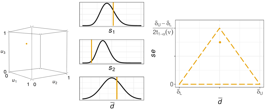
Figure 1: Left: Example point $(0.785,0.009,0.694)\in[0,1]^{3}$. Center: Mapping from this point to sufficient statistics. Right: The rejection region for the TOST procedure.

More generally, sampling distributions for hypothesis tests can be mapped to the unit hypercube $[0,1]^{w}$, where $w$ is the number of sufficient statistics required to compute the relevant test statistics. To design Bayesian posterior analyses, Hagar and Stevens (2023) leveraged maximum likelihood estimates when low-dimensional sufficient statistics did not exist or were difficult to generate. Those methods rely on large-sample results but could be applied in frequentist settings. The simulation dimension $w$ may be large if using these mappings to design sequential tests with many interim analyses or facilitate extensive multi-group comparisons. If $w\geq 32$, caution should be exercised when using quasi-Monte Carlo methods; high-dimensional low-discrepancy sequences may have poor low-dimensional projections, which can lead to a deterioration in performance (Lemieux, 2009). Pseudorandom sequences could instead be used to implement such large-dimensional mappings.

For two-group equivalence tests, power analysis could be implemented by estimating power via Algorithm 1 at various sample sizes until the desired study power of $1-\beta$ is achieved for some type II error rate $\beta$. However, that approach would be inefficient since we would need to thoroughly explore $[0,1]^{3}$ – and hence estimate the entire sampling distribution – at each combination of sample sizes considered. Low-discrepancy sequences allow us to obtain precise power estimates using fewer points from $[0,1]^{3}$ than pseudorandom sequences, but it would be more efficient to only explore subspaces of $[0,1]^{3}$ that help us estimate power. We develop a methodology for this in Section 3. But first, we introduce an illustrative example that will be used to assess the performance of our method for power curve approximation proposed later. We illustrate the use of Algorithm 1 in this context.

2.2 Illustrative Example

This illustrative example is adapted from PASS 2023 documentation (NCSS, LLC., 2023). PASS is a paid software solution that facilitates power analysis and sample size calculations for two-group equivalence tests with unequal variances. The illustrative example seeks to compare the impact of two drugs on diastolic blood pressure, measured in mmHg (millimeters of mercury). The mean diastolic blood pressure is known to be roughly $\mu_{2}=96$ mmHg with the reference drug $(j=2)$, and it is hypothesized to be about $\mu_{1}=92$ mmHg with the test drug $(j=1)$. Subject matter experts use past studies to hypothesize within-group diastolic blood pressure standard deviations of $\sigma_{1}=18$ mmHg and $\sigma_{2}=15$ mmHg, respectively. The interval endpoints for the study are $\delta_{U}=19.2$ and $\delta_{L}=-\delta_{U}$ to comply with guidance from the United States Food and Drug Administration (FDA, 2006). The significance level for the test is $\alpha=0.05$.

The PASS documentation considers power for the illustrative example at $n=n_{1}=n_{2}=\{3,5,8,10,15,\linebreak 20,30,40,50,60\}$. For each sample size $n$, we estimated power 100 times using Algorithm 1 with $m=2^{16}=65536$. We also obtained 100 empirical power estimates for each sample size $n$ by generating $m$ samples of size $n$ from the $N(\mu_{1},\sigma_{1}^{2})$ and $N(\mu_{2},\sigma_{2}^{2})$ distributions and recording the proportion of samples for which we concluded that $\mu_{1}-\mu_{2}\in(\delta_{L},\delta_{U})$. Table 1 summarizes these numerical results and the power estimates presented in the PASS documentation.

	Estimated Power
$n$	$PASS$	Alg 1	Naïve Simulation
3	0.1073	0.0414 ($1.43\times 10^{-4}$)	0.0414 ($7.85\times 10^{-4}$)
5	0.1778	0.1283 ($1.70\times 10^{-4}$)	0.1282 ($1.27\times 10^{-3}$)
8	0.4094	0.3801 ($2.60\times 10^{-4}$)	0.3800 ($2.03\times 10^{-3}$)
10	0.5527	0.5366 ($2.68\times 10^{-4}$)	0.5368 ($2.03\times 10^{-3}$)
15	0.7723	0.7699 ($1.49\times 10^{-4}$)	0.7700 ($1.88\times 10^{-3}$)
20	0.8810	0.8815 ($1.65\times 10^{-4}$)	0.8816 ($1.39\times 10^{-3}$)
30	0.9679	0.9687 ($9.32\times 10^{-5}$)	0.9688 ($6.66\times 10^{-4}$)
40	0.9924	0.9922 ($5.28\times 10^{-5}$)	0.9922 ($3.24\times 10^{-4}$)
50	0.9982	0.9982 ($3.45\times 10^{-5}$)	0.9982 ($1.67\times 10^{-4}$)
60	0.9996	0.9996 ($2.10\times 10^{-5}$)	0.9996 ($7.22\times 10^{-5}$)

Table 1: Power estimates presented in the $PASS$ documentation along with the mean of 100 empirical power estimates obtained via Algorithm 1 (Alg 1) and simulating normal data (Naïve Simulation). Standard deviations of the 100 empirical power estimates are given in parentheses.

The two simulation-based approaches provide unbiased power estimates. However, Table 1 shows that the power estimates obtained via Algorithm 1 are much more precise than those obtained via naïve simulation with pseudorandom sequences. Moreover, each power estimate was obtained in roughly a quarter of a second when using Algorithm 1. It took between 20 and 30 seconds to obtain each power estimate using naïve simulation. This occurs because – regardless of the sample size $n$ considered – Algorithm 1 reduces the power calculation to a three-dimensional problem that can be efficiently vectorized. We must use for loops to estimate power when directly generating the higher-dimensional data $\boldsymbol{y}_{1}$ and $\boldsymbol{y}_{2}$. Moreover, the power estimates presented in the PASS documentation do not coincide with those returned via simulation for sample sizes less than 15, suggesting that alternative methods for power analysis are valuable when the null distribution is not based on pivotal quantities.

3 Power Curve Approximation with Segments of the Sampling Distribution

3.1 An Efficient Approach to Power Analysis

In this section, we leverage the mapping between the unit cube and the test statistics presented in Section 2 to facilitate power curve approximation while estimating only segments of the sampling distribution. For given sample sizes $n_{1}$ and $n_{2}$, we previously mapped each Sobol’ sequence point $\boldsymbol{u}_{r}$ ($r=1,...,m$) to a mean difference, standard error, and degrees of freedom for its test statistic: $\bar{d}_{r}$, $se_{r}$, and $\nu_{r}$. To compute empirical power in Algorithm 1, we fixed the sample sizes $n_{1}$ and $n_{2}$ and allowed the Sobol’ sequence point to vary. We now specify a constant $q>0$ such that $n=n_{1}=qn_{2}$ to allow for imbalanced sample sizes. When approximating the power curve, we fix the Sobol’ sequence point $\boldsymbol{u}_{r}$ and let the sample size $n$ vary. We introduce the notation $\bar{d}_{r}^{{}_{(n,q)}}$, $se_{r}^{{}_{(n,q)}}$, and $\nu_{r}^{{}_{(n,q)}}$ to make this clear. For fixed $q$ and $r$, these quantities are only functions of the sample size $n$. As $n\rightarrow\infty$, $\bar{d}_{r}^{{}_{(n,q)}}$, $se_{r}^{{}_{(n,q)}}$, and $\nu_{r}^{{}_{(n,q)}}$ approach $\mu_{1}-\mu_{2}$, 0, and $\infty$, respectively.

We consider the behaviour of these functions when $H_{1}$ is true, i.e., when $\mu_{1}-\mu_{2}\in(\delta_{L},\delta_{U})$. First, $\nu_{r}^{{}_{(n,q)}}$ almost always increases for fixed $r$ and $q$ as $n$ increases. The upper vertex of the triangular rejection region for the TOST procedure is $\left(0.5\hskip 0.25pt(\delta_{L}+\delta_{U}),0.5\hskip 0.25pt(\delta_{U}-\delta_{L})/t_{1-\alpha}(\nu_{r}^{{}_{(n,q)}})\right)$. As $n\rightarrow\infty$, the vertical coordinate of this vertex increases to $0.5\hskip 0.25pt(\delta_{U}-\delta_{L})/\Phi^{-1}({1-\alpha})$, and the remaining two vertices do not change. The rejection region defines a threshold for the standard error $se_{r}^{{}_{(n,q)}}$: $\Lambda_{r}^{{}_{(n,q)}}=\text{min}\{\bar{d}_{r}^{{}_{(n,q)}}-\delta_{L},\delta_{U}-\bar{d}_{r}^{{}_{(n,q)}}\}/t_{1-\alpha}(\nu_{r}^{{}_{(n,q)}})$. We conclude $\mu_{1}-\mu_{2}\in(\delta_{L},\delta_{U})$ if and only if $se_{r}^{{}_{(n,q)}}$ does not exceed this threshold. For fixed $r$ and $q$, this threshold is also a function of $n$:

$$\Lambda_{r}^{{}_{(n,q)}}:=\begin{cases*}\dfrac{(\mu_{1}-\mu_{2})-\delta_{L}}{t_{1-\alpha}(\nu_{r}^{{}_{(n,q)}})}+\dfrac{\Phi^{-1}(u_{3r})\sqrt{\sigma_{1}^{2}+\sigma_{2}^{2}/q}}{\sqrt{n}\hskip 0.25ptt_{1-\alpha}(\nu_{r}^{{}_{(n,q)}})}&if $\delta_{L}<\bar{d}_{r}^{{}_{(n,q)}}\leq 0.5\hskip 0.25pt(\delta_{L}+\delta_{U})$\\ \dfrac{\delta_{U}-(\mu_{1}-\mu_{2})}{t_{1-\alpha}(\nu_{r}^{{}_{(n,q)}})}-\dfrac{\Phi^{-1}(u_{3r})\sqrt{\sigma_{1}^{2}+\sigma_{2}^{2}/q}}{\sqrt{n}\hskip 0.25ptt_{1-\alpha}(\nu_{r}^{{}_{(n,q)}})}&if $0.5\hskip 0.25pt(\delta_{L}+\delta_{U})<\bar{d}_{r}^{{}_{(n,q)}}<\delta_{U}$\\ 0&\text{otherwise.}\end{cases*}$$ (4)

We suppose that a given point $\boldsymbol{u}_{r}$ yields $se_{r}^{{}_{(n,q)}}\leq\Lambda_{r}^{{}_{(n,q)}}$, which corresponds to the rejection region of the TOST procedure. In Appendix A, we discuss why $se_{r}^{{}_{(n+1,q)}}\leq\Lambda_{r}^{{}_{(n+1,q)}}$ generally also holds true for the same point $\boldsymbol{u}_{r}$. In light of this, our method to approximate the power curve generates a single Sobol’ sequence of length $m$. We use root-finding algorithms (Brent, 1973) to find the smallest value of $n$ such that $se_{r}^{{}_{(n,q)}}\leq\Lambda_{r}^{{}_{(n,q)}}$ for each point $r=1,...,m$. We use the empirical CDF of these $m$ sample sizes to approximate the power curve as described in Algorithm 2.

Algorithm 2 Procedure for Power Curve Approximation

1:procedure PowerCurve($\mu_{1}-\mu_{2},\sigma_{1},\sigma_{2},\delta_{L},\delta_{U},\alpha$, $\beta$, $q$, $m$)

2:     sampSobol $\leftarrow\textsc{null}$

3:     for $r$ in 1:$m$ do

4:         Generate Sobol’ sequence point $\boldsymbol{u}_{r}$

5:         Let $\texttt{sampSobol}[r]$ solve $se_{r}^{{}_{(n,q)}}-\Lambda_{r}^{{}_{(n,q)}}=0$ in terms of $n$      

6:     Let $n_{*}$ be the $(1-\beta)$-quantile of sampSobol

7:     for $r$ in 1:$m$ do

8:         if $\texttt{sampSobol}[r]\leq n_{*}$ then

9:              if $se_{r}^{{}_{(n,q)}}>\Lambda_{r}^{{}_{(n,q)}}$ then

10:                  Repeat Line 5, initializing the root-finding algorithm at $n_{*}$               

11:         else

12:              if $se_{r}^{{}_{(n,q)}}\leq\Lambda_{r}^{{}_{(n,q)}}$ then

13:                  Repeat Line 5, initializing the root-finding algorithm at $n_{*}$                             

14:     $\texttt{powerCurve}\leftarrow$ empirical CDF of sampSobol

15:     Let $n^{*}$ be the $(1-\beta)$-quantile of sampSobol

16:     return powerCurve, $n_{1}=\lceil n^{*}\rceil$ and $n_{2}=\lceil qn^{*}\rceil$ as the recommended sample sizes

We now elaborate on several of the steps in Algorithm 2. Lines 2 to 6 describe a process that would yield an unbiased power curve and sample size recommendation if $se_{r}^{{}_{(n,q)}}=\Lambda_{r}^{{}_{(n,q)}}$ were guaranteed to have a unique solution in terms of $n$ for fixed $r$ and $q$. However, $se_{r}^{{}_{(n,q)}}$ and $\Lambda_{r}^{{}_{(n,q)}}$ may infrequently intersect more than once. Given the reasoning in Appendix A and the numerical studies in Section SM1 of the online supplement, these multiple intersections do not occur frequently enough to deter us from using root-finding algorithms to explore sample sizes. With root-finding algorithms, we explore only subspaces of $[0,1]^{3}$ for each sample size investigated since different values of $n$ are considered for each point $\boldsymbol{u}_{r}$ in Line 4. Root-finding algorithms therefore give rise to computational efficiency as the entire sampling distribution is not estimated when exploring sample sizes $n$. In particular, the root-finding algorithm computes test statistics corresponding to $\mathcal{O}(\text{log}_{2}B)$ points from $[0,1]^{3}$, where $B$ is the maximum sample size considered for the power curve. We would require $\mathcal{O}(B)$ such points to explore a similar range of sample sizes using power estimates from Algorithm 1. When $B\geq 59$, this approach reduces the number of test statistics we must estimate by at least an order of magnitude because $\mathcal{O}(\text{log}_{2}B)<\mathcal{O}(B)/10$. Using low-discrepancy sequences instead of pseudorandom ones further reduces the number of test statistics we must estimate as demonstrated in Section 3.2.

If we skipped Lines 7 to 14 of Algorithm 2, the unbiasedness of the sample size recommendation in Line 16 is not guaranteed due to the potential for multiple intersections between $se_{r}^{{}_{(n,q)}}$ and $\Lambda_{r}^{{}_{(n,q)}}$. To ensure our sample size recommendations are unbiased despite using subspaces of $[0,1]^{3}$ to consider sample sizes, we estimate the entire sampling distribution of test statistics at the sample size $n=n_{*}$ in Lines 7 to 13. If the statements in Lines 9 or 12 are true, this implies that $se_{r}^{{}_{(n,q)}}=\Lambda_{r}^{{}_{(n,q)}}$ for at least two distinct sample sizes $n$. For these points $\boldsymbol{u}_{r}$, we can reinitialize the root-finding algorithm at $n_{*}$ to obtain a solution for each point that will make the power curve unbiased at $n_{*}$. Our numerical studies in Section 3.2 show that the if statements in Lines 9 and 12 are very rarely true for any point $\boldsymbol{u}_{r}\in[0,1]^{3}$. In those situations, $n_{*}=n^{*}$ and both the power estimate at $n^{*}$ and the sample size recommendations $\lceil n^{*}\rceil$ and $\lceil qn^{*}\rceil$ are unbiased. It is incredibly unlikely that $n_{*}$ and $n^{*}$ would differ substantially, but Lines 7 to 13 of Algorithm 2 could be repeated in that event, where the root-finding algorithm is initialized at $n^{*}$ instead of $n_{*}$. Even when $se_{r}^{{}_{(n,q)}}$ and $\Lambda_{r}^{{}_{(n,q)}}$ intersect more than once, the power curves from Algorithm 2 are unbiased near the target power $1-\beta$, but their global unbiasedness at all sample sizes $n$ is not strictly guaranteed. Nevertheless, our numerical studies in Section 3.2 highlight good global estimation of the power curve.

The methods we leveraged to select subspaces of $[0,1]^{3}$ for two-group equivalence tests are tailored to the functions $se_{r}^{{}_{(n,q)}}$ and $\Lambda_{r}^{{}_{(n,q)}}$. However, these methods rely more generally on the weak law of large numbers since most sufficient statistics are based on sample means. Upon mapping the unit hypercube $[0,1]^{w}$ to sufficient statistics, the behaviour of the test statistics as a function of the sample size $n$ can generally be studied to develop analogs to Algorithm 2 for other tests and designs. Root-finding algorithms are generally useful when the rejection region is convex. Rejection regions for the TOST procedure in Figure 1, other equivalence tests, and one-sided hypothesis tests are typically convex, whereas hypothesis tests with point null hypotheses often have non-convex rejection regions.

3.2 Numerical Study with the Illustrative Example

We reconsider the illustrative example from Section 2.2 to illustrate the reliable performance of our efficient method for power curve approximation. For this example, we approximate the power curve 1000 times with $q=1$ (i.e., $n=n_{1}=n_{2}$). Each of the 1000 power curves are approximated using Algorithm 2 with a target power of $1-\beta=0.8$ and a Sobol’ sequence of length $m=2^{10}=1024$. We recommend using shorter Sobol’ sequences when approximating the power curve than when computing empirical power for a specific $(n_{1},n_{2})$ combination ($m=65536$ was used in Section 2.2). Whereas all computations in Algorithm 1 can be vectorized, we must use a for loop to implement the root-finding algorithm for each Sobol’ sequence point. We compare these 1000 power curves to the unbiased power estimates from Algorithm 1 in Table 1. The left plot of Figure 2 demonstrates that Algorithm 2 yields suitable global power curve approximation when comparing its results to these power estimates.

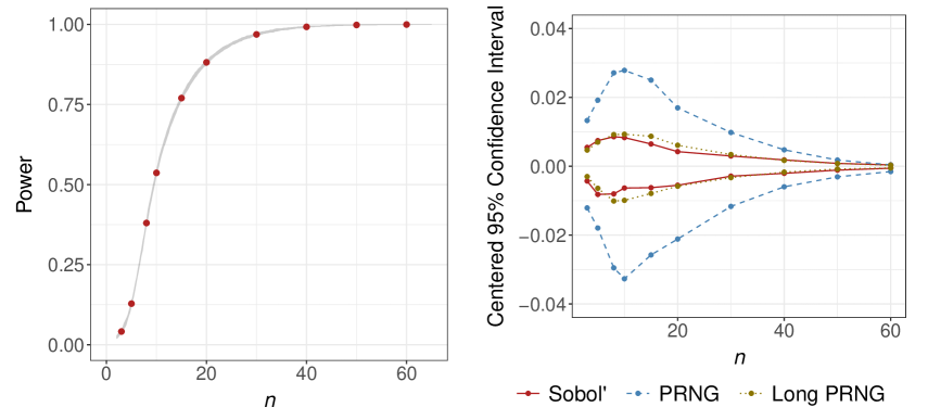
Figure 2: Left: 1000 power curves estimated for the illustrative example (gray) and the power estimates obtained via Algorithm 1 (red). Right: Endpoints of the centered 95% confidence intervals for power obtained with Sobol’ ($m=1024$) and pseudorandom (PRNG) sequences ($m=1024,10^{4})$.

Each power curve was approximated without estimating the entire sampling distribution for all sample sizes $n_{1}$ and $n_{2}$ explored as emphasized in Section 3.3. To further investigate the performance of Algorithm 2, we repeated the process from the previous paragraph to estimate 1000 power curves for the illustrative example with $1-\beta=\{0.2,0.3,\dots,0.7,0.9\}$. In total, we approximated 8000 power curves for this example. Using the root-finding algorithm to explore the sample size space did not lead to performance issues. We did not need to reinitialize the root-finding algorithm in Lines 7 to 13 of Algorithm 2 for any of the $8.192\times 10^{6}$ points used to generate these 8000 curves. The suitable performance of Algorithm 2 is corroborated by more extensive numerical studies detailed in Section SM1 of the online supplement.

To assess the impact of using Sobol’ sequences with Algorithm 2, we approximated 1000 power curves for the illustrative example using root-finding algorithms with $1-\beta=0.8$ and sequences from a pseudorandom number generator. We then used the 1000 power curves corresponding to each sequence type (Sobol’ and pseudorandom) to estimate power for the sample sizes considered in Section 2.2: $n=\{3,5,8,10,15,20,30,40,$ $50,60\}$. For each sample size and sequence type, we obtained a 95% confidence interval for power using the percentile bootstrap method (Efron, 1982). We then created centered confidence intervals by subtracting the power estimates produced by Algorithm 1 from each confidence interval endpoint. The right plot of Figure 2 depicts these results for the 10 sample sizes $n$ and two sequence types considered. Figure 2 illustrates that the Sobol’ sequence gives rise to much more precise power estimates than pseudorandom sequences – particularly when power is not near 0 or 1. We repeated this process to generate 1000 power curves via Algorithm 2 with pseudorandom sequences of length $m=10^{4}$. The power estimates obtained using Sobol’ sequences with length $m=1024$ are roughly as precise as those obtained with pseudorandom sequences of length $m=10^{4}$. Using Sobol’ sequences therefore allows us to estimate power with the same precision using approximately an order of magnitude fewer points from $[0,1]^{3}$. Each power curve for this example with $m=1024$ took just under one second to approximate. It would take roughly 10 times as long to approximate the power curve with the same precision using pseudorandom points in lieu of Sobol’ sequences.

3.3 Exploring Subspaces of the Unit Cube

Here, we demonstrate how segments of the sampling distribution are estimated by exploring only subspaces of the unit cube $[0,1]^{3}$ for most sample sizes considered. The left plot of Figure 3 decomposes the results of the root-finding algorithm for one approximated power curve from Section 3.2 with $1-\beta=0.8$ for the illustrative example. Even when the root-finding algorithm is initialized at the same sample size for all $\{\boldsymbol{u}_{r}\}_{r=1}^{m}$, different $n$ are considered for each point $\boldsymbol{u}_{r}$ when determining the solution to $se_{r}^{{}_{(n,q)}}=\Lambda_{r}^{{}_{(n,q)}}$. The value of $n$ is noninteger in most iterations of the root-finding algorithm, and the colors in the left plot of Figure 3 indicate which points from the unit cube were considered for various ranges of $n$. For instance, the purple points were such that their test statistics corresponded to the rejection region for the smallest possible sample size of $n=2$. Moreover, only the blue points in $[0,1]^{3}$ were used to estimate test statistics for at least one sample size $n\in(2,8)$ when exploring values of $n$ via the root-finding procedure.

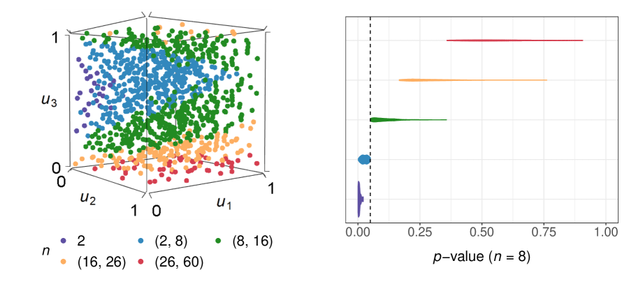
Figure 3: Left: Visualization of which points in $[0,1]^{3}$ were used to explore at least one $n$ value in the various sample size ranges via the root-finding algorithm. Right: Violin plots for the sampling distribution of $p$-values corresponding to $n=8$ conditional on the colored categorization of points. The dotted vertical line is at $\alpha=0.05$.

The points that were used to explore the smallest sample sizes generally have moderate $u_{3r}$ values and smaller $u_{1r}$ and $u_{2r}$ values. The mean difference $\bar{d}_{r}^{{}_{(n,q)}}$ is therefore small in absolute value and the sample variances for groups 1 and 2 are small, which implies that the numerators of the test statistics $t_{L}$ and $t_{U}$ are large and their denominators are small. The points used to explore larger sample sizes generally have more extreme $u_{3r}$ values, so $\bar{d}_{r}^{{}_{(n,q)}}$ may not substantially differ from one of $\delta_{L}$ or $\delta_{U}$ for small sample sizes. While the pattern in the left plot of Figure 3 depends on the inputs for Algorithm 2, the root-finding algorithm correctly identifies which subspaces of $[0,1]^{3}$ to prioritize for a given sample size $n$ with an arbitrary design. Our methods can be extended to more complex designs, but it is difficult to visualize the prioritized subspaces of the unit hypercube when the simulation dimension $w$ is greater than 3.

The right plot of Figure 3 visualizes the sampling distribution of $p$-values for $n=n_{1}=n_{2}=8$ conditional on the categorizations from the left plot. For the TOST procedure, the $p$-value is the maximum of the $p$-values corresponding to $t_{L}$ and $t_{U}$. This $p$-value does not exceed the significance level $\alpha$ if and only if $se_{r}^{{}_{(n,q)}}\leq\Lambda_{r}^{{}_{(n,q)}}$. This plot demonstrates why it is wasteful to use the purple points to consider $n\approx 8$ because those points satisfy $se_{r}^{{}_{(n,q)}}\leq\Lambda_{r}^{{}_{(n,q)}}$ for $n=2$. It follows from Appendix A that $se_{r}^{{}_{(n,q)}}\leq\Lambda_{r}^{{}_{(n,q)}}$ generally holds true for $n\approx 8$ with those points, and the corresponding $p$-values are hence smaller than $\alpha=0.05$. By similar logic, it is wasteful to consider the red points for $n\approx 8$ since the $p$-values for those points will be much larger than $\alpha$. Although these colored categorizations are not used in Algorithm 2, they illustrate the targeted nature of how we consider sample sizes $n$ with segments of the relevant sampling distributions.

4 Discussion

In this paper, we developed a framework for power analysis when null distributions cannot be expressed in terms of pivotal quantities. This framework maps the unit hypercube $[0,1]^{w}$ to sufficient statistics and leverages this mapping to estimate power curves using segments of sampling distributions. Using segments of sampling distributions improves the scalability of our simulation-based design procedures without compromising the unbiasedness of the sample size recommendations. Our framework is illustrated with three-dimensional simulation for two-group equivalence tests with unequal variances, but we described how to apply our methods more generally throughout the paper and now elaborate on several such extensions.

Future work could apply the framework proposed in this paper to crossover designs, where each observation may be subjected to multiple experimental conditions. Under normality assumptions, the relevant means and variances are those for contrasts of the effects in various conditions. To apply this framework to compare more than two groups, the simulation dimension $w$ would need to be increased, and the multiple comparisons problem would need to be considered. We could also apply this framework to efficiently design sequential analyses that allow for early termination of the study. In sequential settings, we would likely need to define analogues to $se_{r}^{{}_{(n,q)}}$ and $\Lambda_{r}^{{}_{(n,q)}}$ for each interim analysis and synthesize the results for each point $\boldsymbol{u}_{r}$. However, it is not trivial to create a mapping between points in $[0,1]^{w}$ and sufficient statistics that maintain the desired level of dependence between interim analyses for arbitrary sample sizes.

Finally, we could explore how this framework might be applied to quickly and reliably recommend sample sizes for nonparametric testing methods. The exact null distributions for those tests are not based on pivotal quantities, and it is not possible to generate sufficient statistics in nonparametric settings. Sample size determination for these studies typically utilizes naïve simulation. In nonparametric settings, we may be able to map the unit hypercube $[0,1]^{w}$ to insufficient statistics, such as sample totals, and use low-discrepancy sequences to improve the scalability and precision of empirical power analysis.

Supplementary Material

These materials detail additional numerical studies and discussion of competing approaches for power analysis. The code to conduct the numerical studies in the paper is available online: https://github.com/github-anonymous-author/PowerNoPivots.

Funding Acknowledgement

This work was supported by the Natural Sciences and Engineering Research Council of Canada (NSERC) by way of a PGS D scholarship as well as Grant RGPIN-2019-04212.

Appendix A Justification for Using Root-Finding Algorithms

Here, we discuss why using root-finding algorithms to approximate the power curve yields suitable results – even though $se_{r}^{{}_{(n,q)}}$ and $\Lambda_{r}^{{}_{(n,q)}}$ can (although infrequently) intersect more than once. The threshold $\Lambda_{r}^{{}_{(n,q)}}$ approaches $\Lambda^{*}=\text{min}\{(\mu_{1}-\mu_{2})-\delta_{L},\delta_{U}-(\mu_{1}-\mu_{2})\}/\Phi^{-1}({1-\alpha})>0$ as $n$ increases. The standard error $se_{r}^{{}_{(n,q)}}$ generally decreases as $n\rightarrow\infty$, but it is not necessarily a strictly decreasing function of $n$. We first consider the case where $se_{r}^{{}_{(n,q)}}$ does strictly decrease as $n$ increases. For small sample sizes, $\Lambda_{r}^{{}_{(n,q)}}$ is typically an increasing function of $n$ due to the decrease in $t_{1-\alpha}(\nu_{r}^{{}_{(n,q)}})$. If the Sobol’ sequence point $\boldsymbol{u}_{r}$ is such that $\text{sign}(u_{3r}-0.5)=\text{sign}((\mu_{1}-\mu_{2})-0.5\hskip 0.25pt(\delta_{L}+\delta_{U}))$, then $\Lambda_{r}^{{}_{(n,q)}}$ is also an increasing function of $n$ for large sample sizes. This occurs because $\bar{d}_{r}^{{}_{(n,q)}}$ is never closer than $\mu_{1}-\mu_{2}$ to the horizontal center of the rejection region at $\bar{d}=0.5\hskip 0.25pt(\delta_{L}+\delta_{U})$. Therefore, the increasing $\Lambda_{r}^{{}_{(n,q)}}$ and decreasing $se_{r}^{{}_{(n,q)}}$ typically intersect once. If $\text{sign}(u_{3r}-0.5)\neq\text{sign}((\mu_{1}-\mu_{2})-0.5\hskip 0.25pt(\delta_{L}+\delta_{U}))$, then $\Lambda_{r}^{{}_{(n,q)}}$ is a decreasing function of $n$ for large sample sizes. This occurs because $\bar{d}_{r}^{{}_{(n,q)}}$ approaches $\mu_{1}-\mu_{2}$ from the horizontal center of the rejection region. However, $\Lambda_{r}^{{}_{(n,q)}}$ decreases to a nonzero constant $\Lambda^{*}$, while $se_{r}^{{}_{(n,q)}}$ decreases to 0 as $n\rightarrow\infty$. Again, the functions $\Lambda_{r}^{{}_{(n,q)}}$ and $se_{r}^{{}_{(n,q)}}$ typically intersect only once.

We next consider the case where $se_{r}^{{}_{(n,q)}}$ is not a strictly decreasing function of $n$. Line 5 of Algorithm 1 prompts the first line of (A):

$$se_{r}^{{}_{(n,q)}} = \dfrac{1}{\sqrt{n}}\left[\dfrac{\sigma_{1}^{2}}{n-1}F(u_{1r};n-1)+\dfrac{\sigma_{2}^{2}}{q(qn-1)}F(u_{2r};qn-1)\right]^{1/2}$$

$$\approx \dfrac{1}{\sqrt{2n}}\left[\dfrac{\sigma_{1}^{2}}{n-1}\left(\Phi^{-1}(u_{1r})+\sqrt{2(n-1)}\right)^{2}+\dfrac{\sigma_{2}^{2}}{q(qn-1)}\left(\Phi^{-1}(u_{2r})+\sqrt{2(qn-1)}\right)^{2}\right]^{1/2}.$$

Because quantiles from the chi-squared distribution do not have closed forms, the second line of (A) leverages the approximation from Fisher (1934) for illustrative purposes. When $\Phi^{-1}(u_{1r})\in(-\sqrt{2(n-1)}\pm 1)$ or $\Phi^{-1}(u_{2r})\in(-\sqrt{2(qn-1)}\pm 1)$, the square function respectively makes the $(\Phi^{-1}(u_{1r})+\sqrt{2(n-1)})^{2}$ or $(\Phi^{-1}(u_{2r})+\sqrt{2(qn-1)})^{2}$ term in (A) smaller. As $n$ increases in those situations, the relative increase in the squared terms may offset the decreasing impact of the terms in the denominators of (A). However, this increasing trend cannot persist as $se_{r}^{{}_{(n,q)}}$ is $O\left(n^{-\frac{1}{2}}\right)$ and $Pr(\Phi^{-1}(u_{1r})\in(-\sqrt{2(n-1)}\pm 1))$ and $Pr(\Phi^{-1}(u_{2r})\in(-\sqrt{2(qn-1)}\pm 1))$ both approach 0 as $n\rightarrow\infty$. We show via simulation in Section SM1 of the online supplement that this increasing trend is rare for $n>5$. For $n\leq 5$, $\Lambda_{r}^{{}_{(n,q)}}$ is generally also an increasing function of $n$ as mentioned in Section 3.1.

If $\Lambda_{r}^{{}_{(n,q)}}$ is a decreasing function of $n$, it follows from (4) that $\bar{d}_{r}^{{}_{(n,q)}}=0.5\hskip 0.25pt(\delta_{L}+\delta_{U})$ when

$$n=\dfrac{(\Phi^{-1}(u_{3r}))^{2}(\sigma_{1}^{2}+\sigma_{2}^{2}/q)}{(0.5\hskip 0.25pt(\delta_{L}+\delta_{U})-(\mu_{1}-\mu_{2}))^{2}}.$$ (A2)

The threshold $\Lambda_{r}^{{}_{(n,q)}}$ should therefore not be decreasing for sample sizes smaller than $n$ given in (A2). By (A), $se_{r}^{{}_{(n,q)}}$ approximates $n^{-\frac{1}{2}}\sqrt{\sigma_{1}^{2}+\sigma_{2}^{2}/q}$ for large sample sizes $n$. It follows by (4) that

$$\Lambda_{r}^{{}_{(n,q)}}\approx\Lambda^{*}+\dfrac{\lvert\Phi^{-1}(u_{3r})\rvert}{\Phi^{-1}(1-\alpha)}se_{r}^{{}_{(n,q)}},$$ (A3)

when $\text{sign}(u_{3r}-0.5)\neq\text{sign}((\mu_{1}-\mu_{2})-0.5\hskip 0.25pt(\delta_{L}+\delta_{U}))$ for large $n$. We note that $\Lambda_{r}^{{}_{(n,q)}}$ and $se_{r}^{{}_{(n,q)}}$ may intersect for a value of $n$ that is smaller than the one given in (A2). If $se_{r}^{{}_{(n,q)}}$ is instead larger than $\Lambda_{r}^{{}_{(n,q)}}$ over the entire range of $n$ values for which $\Lambda_{r}^{{}_{(n,q)}}$ increases, then (A3) suggests that $\Lambda_{r}^{{}_{(n,q)}}$ and $se_{r}^{{}_{(n,q)}}$ are likely to intersect only once when $\Lambda_{r}^{{}_{(n,q)}}$ is decreasing. The functions $se_{r}^{{}_{(n,q)}}$ and $\Lambda_{r}^{{}_{(n,q)}}$ therefore typically have one intersection for all cases discussed in this appendix, but we illustrate an occurrence of multiple intersections in Section SM1 of the online supplement.

References

- Brent (1973) Brent, R. P. (1973). An algorithm with guaranteed convergence for finding the minimum of a function of one variable. Algorithms for Minimization without Derivatives, Prentice-Hall, Englewood Cliffs, NJ, 61–80.
- Chow and Liu (2008) Chow, S. C. and J. P. Liu (2008). Design and Analysis of Bioavailability and Bioequivalence Studies. Chapman and Hall/CRC.
- Chow et al. (2008) Chow, S. C., J. Shao, and H. Wang (2008). Sample size calculations in clinical research. Chapman & Hall/CRC.
- Dannenberg et al. (1994) Dannenberg, O., H. Dette, and A. Munk (1994). An extension of Welch’s approximate t-solution to comparative bioequivalence trials. Biometrika 81(1), 91–101.
- Efron (1982) Efron, B. (1982). The jackknife, the bootstrap and other resampling plans. SIAM.
- FDA (2006) FDA (2006). Guidance for industry - Bioequivalence guidance. Center for Drug Evaluation and Research, U.S. Food and Drug Administration, Rockville, MD.
- Fisher (1934) Fisher, R. A. (1934). Statistical methods for research workers (5th ed.). Oliver and Boyd, Edinburgh and London.
- Gruman et al. (2007) Gruman, J. A., R. Cribbie, and C. A. Arpin-Cribbie (2007). The effects of heteroscedasticity on tests of equivalence. Journal of Modern Applied Statistical Methods 6(1), 133–140.
- Hagar and Stevens (2023) Hagar, L. and N. T. Stevens (2023). Fast power curve approximation for posterior analyses. https://arxiv.org/abs/2310.12427.
- Hofert and Lemieux (2020) Hofert, M. and C. Lemieux (2020). qrng: (Randomized) Quasi-Random Number Generators. R package version 0.0-8.
- Jan and Shieh (2017) Jan, S.-L. and G. Shieh (2017). Optimal sample size determinations for the heteroscedastic two one-sided tests of mean equivalence: Design schemes and software implementations. Journal of Educational and Behavioral Statistics 42(2), 145–165.
- Lemieux (2009) Lemieux, C. (2009). Using quasi–monte carlo in practice. In Monte Carlo and Quasi-Monte Carlo Sampling, pp. 1–46. Springer.
- Lui (2016) Lui, K.-J. (2016). Crossover Designs: Testing, Estimation, and Sample Size. John Wiley & Sons.
- NCSS, LLC. (2023) NCSS, LLC. (2023). Chapter 529 - Two-sample t-tests for equivalence allowing unequal variance. Power Analysis and Sample Size (PASS) 2023 Documentation. https://www.ncss.com/wp-content/themes/ncss/pdf/Procedures/PASS/Two-Sample_T-Tests_for_Equivalence_Allowing_Unequal_Variance.pdf.
- Rusticus and Lovato (2014) Rusticus, S. A. and C. Y. Lovato (2014). Impact of sample size and variability on the power and type i error rates of equivalence tests: A simulation study. Practical Assessment, Research, and Evaluation 19(1), 11.
- Satterthwaite (1946) Satterthwaite, F. E. (1946). An approximate distribution of estimates of variance components. Biometrics bulletin 2(6), 110–114.
- Schuirmann (1981) Schuirmann, D. J. (1981). On hypothesis-testing to determine if the mean of a normal-distribution is contained in a known interval [abstract]. Biometrics 37(3), 617.
- Shao (2003) Shao, J. (2003). Mathematical statistics. Springer Science & Business Media.
- Sobol’ (1967) Sobol’, I. M. (1967). On the distribution of points in a cube and the approximate evaluation of integrals. Zhurnal Vychislitel’noi Matematiki i Matematicheskoi Fiziki 7(4), 784–802.
- Tartakovsky et al. (2015) Tartakovsky, A., I. Nikiforov, and M. Basseville (2015). Sequential Analysis: Hypothesis Testing and Changepoint Detection. CRC press.
- Welch (1938) Welch, B. L. (1938). The significance of the difference between two means when the population variances are unequal. Biometrika 29(3/4), 350–362.
- Welch (1947) Welch, B. L. (1947). The generalization of ‘Student’s’ problem when several different population varlances are involved. Biometrika 34(1-2), 28–35.
- Welch (1951) Welch, B. L. (1951). On the comparison of several mean values: an alternative approach. Biometrika 38(3/4), 330–336.