Feeding and feedback processes in the Spiderweb proto-intracluster medium

Abstract

Context. We present a detailed analysis of the thermal, diffuse emission of the proto-intracluster medium (proto-ICM) detected in the halo of the Spiderweb Galaxy at $z=2.16,$ within a radius of $\sim$ 150 kpc.

Aims. Our main goal is to derive the thermodynamic profiles of the proto-ICM, establish the potential presence of a cool core and constrain the classical mass deposition rate (MDR) that may feed the nuclear and the star formation (SF) activity, and estimate the available energy budget of the ongoing feedback process.

Methods. We combined deep X-ray data from Chandra and millimeter observations of the Sunyaev-Zeldovich (SZ) effect obtained by the Atacama Large Millimeter/submillimeter Array (ALMA)

Results. Thanks to independent measurements of the pressure profile from the ALMA SZ observation and the electron density profile from the available X-ray data, we derived, for the first time, the temperature profile in the ICM of a $z>2$ protocluster. It reveals the presence of a strong cool core (comparable to local ones) that may host a significant mass deposition flow, consistent with the measured local SF values. We also find mild evidence of an asymmetry in the X-ray surface brightness distribution, which may be tentatively associated with a cavity carved into the proto-ICM by the radio jets. In this case, the estimated average feedback power would be in excess of $\sim 10^{43}$ erg/s. Alternatively, the asymmetry may be due to the young dynamical status of the halo.

Conclusions. The cooling time of baryons in the core of the Spiderweb Protocluster is estimated to be $\sim 0.1$ Gyr, implying that the baryon cycle in the first stages of protocluster formation is characterized by a high-duty cycle and a very active environment. In the case of the Spiderweb protocluster, we are witnessing the presence of a strongly peaked core that is possibly hosting a cooling flow with a MDR up to 250-1000 $\rm M_{\odot}$/year, responsible for feeding both the central supermassive black hole (SMBH) and the high star formation rate (SFR) observed in the Spiderweb Galaxy. This phase is expected to be rapidly followed by active galactic nucleus (AGN) feedback events, whose onset may have already left an imprint in the radio and X-ray appearance of the Spiderweb protocluster, eventually driving the ICM into a self-regulated, long-term evolution in less than one Gyr.

1 Introduction

The progenitors of local galaxy clusters, so-called protoclusters, are rare overdensities at high-redshift ($z>1.5$) that have not become virialized yet, but are expected to reach a total virial mass in the range of $10^{14}-10^{15}\,\rm M_{\odot}$ by $z=0$ (Overzier, 2016). Observations of these large structures, which span breadths of 10$\arcmin$-30$\arcmin$ in the sky (Muldrew et al., 2015), are crucial to investigating the formation of large-scale structures in the Universe, particularly in high-density environments. They will also improve our understanding of the processes of galaxy formation and evolution, the fueling of star formation (SF) and active galactic nuclei (AGNs), as well as the formation of brightest cluster galaxies (BCGs) and the origin and evolution of the ICM, which is the main baryonic component in galaxy clusters.

To date, there has been no consistent, uniform way to search for protoclusters, since they do not reach a high contrast against the foreground and background extragalactic sky across their entire extent. A convenient (albeit potentially biased) technique is to identify high-redshift, massive galaxies inhabiting a local overdensity and/or a very active environment, as a tracer of the full-scale overdensity. In this respect, protocluster search techniques do not differ much from the classic methods used in the search for high-redshift massive clusters, such as identifying concentrations of massive red sequence galaxies (Bell et al., 2004) using near-infrared (NIR) and mid-infrared (MIR) filters (see Gladders & Yee, 2000, 2005; Wilson et al., 2009); searching for extended sources in X-ray surveys (Rosati et al., 2002; Liu et al., 2022) or for the SZ effect associated with the ICM (Carlstrom et al., 2011; Bleem et al., 2015; Mantz et al., 2018; Gobat et al., 2019); investigating the environment around powerful high-redshift radio galaxies (Miley & De Breuck, 2008). In general, for a given protocluster, the average galaxy overdensity on scales of several physical Mpc (possibly comprising the whole region that eventually will collapse and virialize by $z=0$) may be orders of magnitude lower than in virialized clusters. As a consequence, the majority of the diffuse baryons responsible for the X-ray and SZ signal may have not reached a temperature and density sufficient for such systems to be detected with current facilities. Therefore, while in the case of virialized clusters, a single-band observable may be sufficient to efficiently select them and provide a mass scale at the same time, the robust identification and characterization of protoclusters necessarily require a multiwavelength approach.

An unbiased method to identify protoclusters would be the full mapping of the member galaxies across several physical Mpc, but this is clearly extremely time-consuming and not feasible with current observing methods. While the situation is likely to improve with the advent of future large-area surveys in the optical and NIR, such as the Euclid mission (Laureijs et al., 2012) or Rubin Observatory (Ivezić et al., 2019), we have to rely on biased tracers, as previously mentioned. In this respect, enhanced SF and nuclear activity spread across the member galaxies is expected to be a distinctive feature of high-density environments at high redshift. In this scenario, X-ray observations play an important role in studying the unresolved emission of AGNs and, hence, the accretion phenomena onto SMBHs, emission of star-forming galaxies (SFGs), and inverse Compton (IC) emission from the relativistic plasma of the radio jets when present. Furthermore, the X-ray band is key to trace and characterize the proto-ICM that is expected to form and appear during the most intense evolutionary phase of protoclusters in the range $2<z<3$. In particular, it is key to understanding whether the forming proto-ICM reaches densities large enough to give rise to a cooling flow that, in turn, can feed the process of SF in the central halo, usually identified as the BCG undergoing formation. This occurrence seems to be suggested by the high star formation rates (SFRs) measured in proto-BCGs, but the frequency of the cooling flow regime, as well as precipitation and chaotic cold accretion processes (CCA; see Gaspari et al., 2020 for a review), at $z\geq 2,$ have not been measured yet. Another assumption required to strengthen the cooling flow hypothesis at high redshift is that in the very first stages of formation of the main halo, the feedback processes may not have been triggered yet. This would leave room for a significant MDR, at variance with what is commonly observed during the secular evolution of massive clusters at $z<1$, where a fully developed and massive cooling flow with a high and persistent mass-deposition rate has not been observed (Peterson & Fabian, 2006). On the other hand, several processes that may potentially heat the proto-ICM, thereby hampering its cooling, are also occurring on a very short timescales, such as intense SF, merging of comparable-mass subclusters and accretion shocks, as well as AGN jets and associated feedback processes, such as a cascading turbulence (e.g., Gaspari et al., 2018; Wittor & Gaspari, 2020). In this framework, tracing the proto-ICM in the range of $2<z<3$ would provide a wealth of information on a unique and crucial phase of cluster evolution, when many independent physical processes that counterbalance each other occur at very high intensity and on a short timescale.

Needless to say, the X-ray emission from the proto-ICM is expected to be very faint. Models and simulations tell us that at $z>2$ the emission of the proto-ICM is characterized by a very low surface brightness with a small ($\sim 10$ arcsec) extension (Saro et al., 2009). This not only requires high sensitivity, but also high angular resolution ($\leq 1$ arcsec), a feature that is currently provided only by the Chandra satellite. In addition, in the likely case of a protocluster beaconed by a radio galaxy, the thermal emission can be overcome by the non-thermal emission associated with IC scattering of cosmic microwave background (CMB) photons by the relativistic electrons of radio jets.
The only alternative window to observe the proto-ICM with high angular resolution is provided by the SZ effect (Sunyaev & Zeldovich, 1972, 1980). In particular, the thermal SZ effect directly traces the line-of-sight integrated pressure of the free electrons in the diffuse hot baryons. As such, it provides a complementary, yet independent view of the same ICM that can be imaged in emission in the X-ray band (for a review see Mroczkowski et al., 2019). In particular, we note that X-ray data are sensitive mostly to the square of the electron density, while the SZ signal is directly proportional to the pressure; thus, it depends linearly on the electron density. A relevant point is that both the X-ray flux and the SZ signal from the ICM at a given virial mass at high-z do not depend strongly on redshift (Churazov et al., 2015) and, therefore, both windows are well suited to detect the presence of a pressurized plasma out to $z\gtrsim 2$. Clearly, when X-ray and SZ data are available for the same object, thanks to their different dependence on the electron density, the joint analysis of both observables allows us to achieve an improved description of the thermodynamic properties of the ICM (see e.g., Eckert et al., 2019).

In this paper, we focus on the detailed analysis of the protocluster complex surrounding the Spiderweb Galaxy (MRC 1138-262; z=2.156), the first galaxy protocluster for which we have an observational identification of its proto-ICM, provided by both X-ray and SZ data (Tozzi et al., 2022a; Di Mascolo et al., 2023). The Spiderweb protocluster was discovered as an overdensity surrounding an ultra-steep spectrum radio galaxy (Rottgering et al., 1994) with a mass of $10^{12}\,\rm M_{\odot}$, as inferred from the K-band luminosity. This galaxy shows a striking clumpy radio morphology with two jets extending from the central source, which shows clear signs of strong interactions with the surrounding environment (Pentericci et al., 1997). Also, the high rotation measure ($\sim 6000$ rad/m², discovered in Carilli et al., 1997, see also Athreya et al., 1998 and Anderson et al., 2022) confirms the presence of a high-density magnetized plasma. Optical observations classified the Spiderweb as a narrow emission line galaxy at $z=2.156$ (Rottgering et al., 1997), and revealed a clumpy morphology also in the visible band, with a stunning Ly$\alpha$ halo extending up to 200 kpc around the central source with a luminosity of $\sim 4\times 10^{45}$ erg/s (one of the largest known in the Universe). Using spectroscopic observations, Pentericci et al. (2000) discovered 15 Ly$\alpha$ emitters within a projected physical distance of 1.5 Mpc from the central radio galaxy. Also, Kurk et al. (2004b, a) found 40 candidate H$\alpha$ emitters. Finally, Hatch et al. (2009) found at least 19 star-forming protocluster members with stellar masses in the range of $10^{8}-10^{11}$ $M_{\odot}$ within a radius of $\sim$ 150 kpc, which appear to be in the process of merging with the central galaxy (Miley et al., 2006). Recent X-ray Chandra and radio Jansky Very Large Array (JVLA) data allowed our team to confirm a clear spatial correlation between the radio structures and the Ly$\alpha$ emission (Carilli et al., 2022), providing direct evidence for jet-gas interaction. In addition, Chandra data revealed an AGN fraction among the protocluster members with log$(M_{*}/\rm M_{\odot})>10.5$ of 25.5$\pm$4.5$\%$ within a radius of $\sim$ 2.5 Mpc, one of the highest AGN fraction measured in protoclusters and strongly enhanced compared to the field at similar redshift (Tozzi et al., 2022b; Shimakawa et al., 2023). Finally, thermal diffuse emission from a proto-ICM halo with temperature $kT=2.0^{+0.7}_{-0.4}$ keV extending up to a radius of 100 kpc has been identified in the region free from the IC emission associated with the relativistic jets (Tozzi et al., 2022a).

In a study based on data from ALMA (Wootten & Thompson, 2009) and the Atacama Compact Array (ACA, a.k.a. Morita Array; Iguchi et al. 2009), Di Mascolo et al. (2023) reported the detection of the SZ effect showing, in an independent and complementary way, the presence of a nascent ICM within the Spiderweb protocluster. The amplitude and morphology of the detected signal reveal that the SZ effect from the protocluster is lower than expected from dynamical considerations and comparable to that of lower redshift group-scale systems, consistent with expectations for a dynamically active progenitor of a local galaxy cluster. At the same time, this detection clearly shows that current SZ facilities could be used to effectively open a novel observational window onto protocluster environments. As discussed in Di Mascolo et al. (2023), the combination of multi-wavelength data has provided hints for the proto-ICM to be experiencing mergers and dynamical interactions with the large-scale protocluster structure, the Spiderweb galaxy and its extended jets, and, in general, its multi-phase environment.

In this work we present the combined X-ray and SZ analysis of the proto-ICM of the Spiderweb protocluster, providing the first spatially resolved characterization of an ICM halo at $z>2$. The paper is organized as follows. In Section 2, we briefly describe the data acquisition and reduction. In Section 3, we present a detailed analysis of the morphology of the X-ray surface brightness. In Section 4, we describe how we perform the SZ and X-ray data combined analysis. In Section 5, we derive the density, temperature and pressure, entropy and cooling time, and the total and ICM mass profiles of the ICM. In Section 6, we provide an estimate of the energy budget associated with the ongoing feedback processes, the possible presence of a central cooling flow, the possible implications for the high baryon fraction, and, finally, a comparison with other known protoclusters. In Section 7, we comment on the possible extension of this study with SZ facilities from the ground and future X-ray facilities, such as AXIS and STAR-X. Finally, our conclusions are summarized in Section 8. Throughout this paper, we adopt the current Planck cosmology with $\Omega_{m}=0.315$, and $H_{0}=67.4$ km s^-1 Mpc^-1 in a flat geometry (Planck Collaboration et al., 2020). In this cosmology, at $z=2.156$, 1 arcsec corresponds to 8.498 kpc, the Universe is 3.04 Gyr old, and the lookback time is 78% of the age of the Universe. Quoted error bars correspond to a 1$\sigma$ confidence level, unless noted otherwise.

2 Observations and data reduction

2.1 Chandra X-ray data

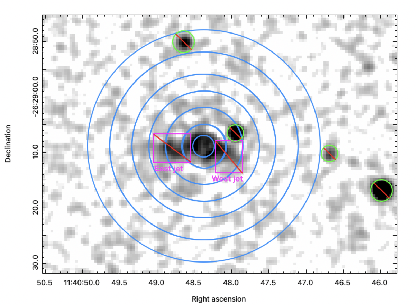
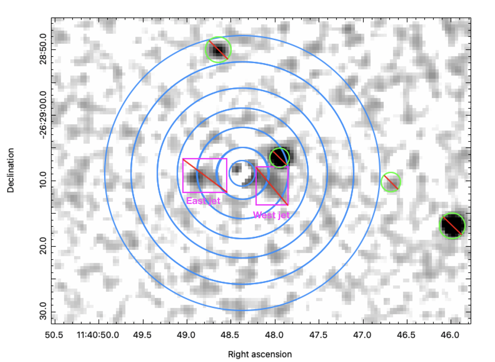
The Spiderweb Galaxy was observed with a Chandra Large Program of 700 ks with ACIS-S (PI: P. Tozzi). The data set includes 21 separate observations obtained in November 2019 through August 2020, plus the first X-ray observation with ACIS-S, dating back to June 2000, for additional 39.5 ks (Carilli et al., 2002). We briefly recall that we run the task acis_process_events with the parameter apply_cti=yes to flag background events, most likely associated with cosmic rays; by rejecting them, we were able to obtain a significant reduction of the background thanks to the VFAINT mode of data acquisition. Thus, we exploited the properties of the VFAINT, ACIS-S data to minimize the noise when deriving the faint surface brightness of the proto-ICM. The final total exposure time after data reduction and excluding the dead-time correction amounts to 715 ks. Full details on observations and data reduction procedure done with CALDB 4.9.3 can be found in Tozzi et al. (2022a). The 22 level-2 event files are eventually merged together with the tool reproject_obs, using the reference coordinates of Obsid 21483. Since this work is focused only on the proto-ICM emission, we used the images where the central AGN had been removed after a careful rendition of the unresolved AGN, as described in Tozzi et al. (2022a). Due to the large luminosity of the AGN, the surface brightness of the diffuse component within a radius of 2 arcsec is not observationally constrained and was treated as a free parameter. We used the parameter $n_{d}$, defined as the ratio of the average surface brightness within a radius of 2 arcsec to the average value measured between 2 and 3.5 arcsec. We used this parameter to quantify our lack of information regarding the diffuse emission within 2 arcsec from the nucleus. Considering that we expect the central surface brightness to be larger than in the outer regions, we have $n_{d}\geq$ 1. We adopted values in the range of 1-6, where $n_{d}$=1 corresponds to a constant surface brightness; namely, $n_{d}\sim 4$ to a developed cool core and $n_{d}\sim 6$ to an extreme cool core. The soft (0.5-2 keV) and hard (2-7 keV) band images in the immediate surroundings ($90\times 70$ arcsec²) of the Spiderweb Galaxy after the AGN subtraction are shown in Figure 1, where we adopted the value $n_{d}=4$ (prominent, but plausibly cool core) as the preferred parametrization of the central surface brightness (see Tozzi et al., 2022a). We do not deconvolve the Chandra PSF when computing the surface brightness profile, since the half energy width is $\sim 0.5$ arcsec, significantly smaller than the minimum width of the annuli we consider here (2 arcsec). In addition, the surface brightness beyond the central region (with a radius of 2 arcsec) is smooth, so that the effect associated with the deconvolution is negligible.

2.2 ALMA+ACA data

The present ALMA and ACA measurement sets comprise multi-band and multi-configuration data, providing a detailed view of the millimeter footprint of the Spiderweb galaxy and its surroundings. In particular, we considered targeted Band 3 ($94.5-110.5\leavevmode\nobreak\ \mathrm{GHz}$) observations obtained by ACA and ALMA (project code: 2018.1.01526.S, PI: A. Saro), spanning $uv$ ranges of $2.2-17.5\leavevmode\nobreak\ \mathrm{k\lambda}$ and $3.93-1320\leavevmode\nobreak\ \mathrm{k\lambda}$, respectively (corresponding to $767-97\leavevmode\nobreak\ \mathrm{kpc}$ and $434-1\leavevmode\nobreak\ \mathrm{kpc}$ at the redshift of the Spiderweb protocluster). To better characterize the spectral properties of the Spiderweb galaxy and exploit the peculiar spectral scaling of the SZ effect for facilitating its separation from the extended radio emission, we complemented the observations with archival Band 4 observations with ALMA (project code: 2015.1.00851.S, PI: B. Emonts) and ACA (project code 2016.2.00048.S, PI: B. Emonts). The data calibration and processing procedures, described in full detail in Di Mascolo et al. (2023) and consisting a standard pipeline calibration applied to all the Band 3 ALMA and ACA data using the Common Astronomy Software Application (CASA). Instead, we obtained the calibrated Band 4 measurement sets through the calMS service (Petry et al., 2020) offered by the European ALMA Regional Centre network (Hatziminaoglou et al., 2015). The direct inspection of all the available data sets did not highlight any issue with the standard calibration, thus, we did not perform any additional calibration, flagging, or post-processing steps.

Finally, we note that in this work, we are interested in inferring solely the large-scale morphology and thermodynamic distribution of the proto-ICM in the Spiderweb protocluster. As such, we considered only the subset of observations below a threshold in $uv$ distance of $65\leavevmode\nobreak\ \mathrm{k\lambda}$. As detailed in Di Mascolo et al. (2023), such a choice makes the extended radio galaxy unresolved along the direction perpendicular to the jet direction. This drastically reduces the morphological components required to model the emission, in turn, simplifying the overall modeling procedure. All the SZ results reported hereafter refer only to the specific $<65\leavevmode\nobreak\ \mathrm{k\lambda}$ subset of ALMA+ACA measurements.

3 Morphology of X-ray emission

As stated in Section 1, in the region free from the jets emission, Tozzi et al. (2022a) ascribed the thermal diffuse X-ray emission to the presence of a proto-ICM halo extending up to a radius of 100 kpc. Indeed, from a visual inspection of the X-ray images, we can immediately identify the diffuse, spherically symmetric emission that is contributed by the proto-ICM in the X-ray soft band (upper left panel of Figure 1), while diffuse emission in the hard band is observed only in correspondence with radio jets; therefore, the latter is dominated by the non-thermal IC emission. As a consequence, as discussed in Tozzi et al. (2022a), we have only a partial view of the surface brightness distribution of the proto-ICM, since in the two regions overlapping with the radio jets, the IC emission originated by the relativistic electrons is larger than the thermal emission in the soft band.

Therefore, in this work we assume that all the diffuse emission outside the jet and AGN regions is associated with the proto-ICM. Nevertheless, we have not been able to firmly exclude a non-thermal contribution. For example, in the case of the radio galaxy 3C294, the extended emission perpendicular to the jets is tentatively associated with IC from an old population of relativistic electrons spread over a large region, due to the precession of the jets on a timescale of 100 Myr (Fabian et al., 2003; Erlund et al., 2006). However, in the Spiderweb galaxy we do no find any hint of jet precession, when, in fact, it should be visible since it would occur on a timescale comparable to the age of the jet (Carilli et al., 2022). In addition, the X-ray surface brightness of the Spiderweb is softer than a typical $\Gamma\sim 2$ power law, and it does not show sharp edges as in the case of 3C294, which is a feature that may be associated with a population of pressure-confined relativistic electrons. Needless to say, we are not able to explore the presence of low surface brightness, roughly isotropic radio emission in our L band JVLA or Giant Metrewave Radio Telescope (GMRT) data, due to the limited dynamic range caused by the presence of the bright radio galaxy. Overall, we recognize that we cannot definitively exclude an IC contribution to the X-ray diffuse emission; however, this scenario is not supported by any observed feature. We go on to discuss the effects of a possible non-thermal contribution in the discussion in Section 6.

Thus, considering the soft, diffuse X-ray emission as entirely associated with the presence of a proto-ICM, we are able to detect such emission only beyond 2 arcsec due to the very high AGN luminosity, while the X-ray luminosity associated with the proto-ICM within 2 arcsec can only be parametrized by assuming a reasonable electron density profile. Clearly, all the other unresolved sources identified in the field are also masked out.

To explore the properties of the X-ray surface brightness associated with the proto-ICM thermal emission, we proceeded according to the following steps: 1) we calculate the number of total counts within specific selected regions in the soft and hard bands, excluding unresolved sources and jet regions; 2) we calculate the area of each selected region after removing the masked areas; 3) we sample the soft and hard band background from a source-free annulus with inner and outer radius of 16 and 29.5 arcsec, respectively, as described in Tozzi et al. (2022a); 4) we calculate the vignetting correction in the soft and hard bands, using the monochromatic exposure maps at 1.5 and 4.5 keV, respectively; 5) we then compute the net detected counts and associated Poissonian uncertainty after subtracting the background rescaled by the geometrical area and applying the vignetting correction; 6) using XSPEC v.12.12.0, we calculate the conversion factor from the count rate to energy flux, assuming a thermal spectrum with $kT=2$ keV and a Galactic absorption of $N_{H}^{Gal}=3.18\times 10^{20}$ cm^-2 according to the HI map of the Milky Way (HI4PI Collaboration et al., 2016); 7) finally, we obtain the average surface brightness of each selected region in units of erg s^-1 cm^-2 arcsec^-2. These steps are synthesized by the relation:

$$SB=ECF\times\frac{(CTS-BCK\times A_{S}/A_{BCK})}{T_{exp}\times A_{S}}\times\frac{Expmap_{Max}}{Expmap_{S}},$$ (1)

where ECF is the energy conversion factor from count rate to energy flux and is equal to $\sim 1.11\times 10^{-12}$ erg/s/cm²/cts; CTS is the number of total counts observed in the image within a given region; BCK is the number of total counts observed in the background region; $A_{S}$ and $A_{BCK}$ are the area values corresponding to the selected region and the background region, respectively; $T_{exp}$ is the total exposure time of the observation after removing the dead time intervals and possible high background rate intervals. The ratio $Expmap_{Max}$/$Expmap_{S}$ is the vignetting correction that is applied to the net counts (observed where the exposure map has the value $Expmap_{S}$) to compute the signal that would be obtained at the aimpoint (where the exposure map reaches the maximum value $Expmap_{Max}$). The maps are computed separately in the soft and hard bands and describe the effective area in $cm^{2}$ at each position in the field of view and, thus, bring the information on the sensitivity of the instruments. Since the signal from the surface brightness is very low, our approach consist in measuring the surface brightness in regions selected specifically to identify possible features of the proto-ICM projected distribution and quantify the corresponding statistical significance.

Figure 1: AGN-subtracted soft (0.5-2 keV, upper left panel) and hard (2-7 keV, upper right panel) band images of the Spiderweb protocluster in a field of view of $\sim$ $90\times 70$ arcsec². The blue concentric circles represent the regions within which we derived the surface brightness and correspond to an outer radius of 2, 4, 7, 10, 13, 17, and 21 arcsec, with the central blue circle showing the region where the unresolved AGN emission makes it impossible to estimate the diffuse emission. The green circles represent removed unresolved sources and the magenta boxes represent the eastern and western jet regions overlapping with the radio emission, and are excluded from our analysis since they are dominated by the diffuse, non-thermal IC emission from the jets. For the purposes of visualization, the central surface brightness is parametrized with $n_{d}=4$, as discussed in Tozzi et al. (2022a). In the lower-left and lower-right panels, we show the corresponding background-subtracted surface brightness profiles computed according to Equation 1. The black bars represent the 1$\sigma$ uncertainties associated with data points including the Poissonian errors on the total counts and the background expected counts. The grey-shaded area marks the value of surface brightness parametrized with $n_{d}=4$ in the first bin and the 1$\sigma$ background level in the other bins.

3.1 Azimuthally averaged profile

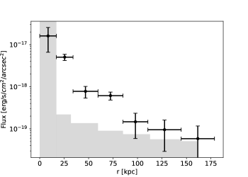
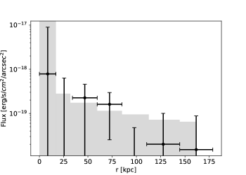
The first step is to derive the surface brightness profile, assuming a spherically symmetric distribution centered on the AGN position (RA=11:40:48.3611 and Dec=-26:29:08.984). Therefore, we extracted the surface brightness profile from seven annuli with outer radius of 2, 4, 7, 10, 13, 17, and 21 arcsec centered on the AGN for the soft and hard images, as shown in the upper panels of Figure 1. Applying Equation 1, we obtain the surface brightness profile in erg/s/cm²/arcsec² in the soft and hard bands, as shown in the lower panels of Figure 1. We find that the azimuthally average surface brightness is well detected in the soft band at radii $r<150$ kpc ($\sim 17$ arcsec), while in the hard band, the photometry is consistent with no signal in all the annuli. These findings confirm that the diffuse emission is entirely soft, consistent with being bremsstrahlung emission with an estimated average temperature of $\sim 2$ keV, as derived from the X-ray spectral analysis in Tozzi et al. (2022a). In the rest of the paper, we work on the soft band image only and we also neglect the data beyond 17 arcsec in the soft band, due to the drastic drop in the number of net counts which could be associated with the ICM.

We also note that the surface brightness profile is strongly increasing towards the center. As said, we are not able to measure the diffuse emission in the innermost region included within a radius of 2 arcsec from the nucleus because of the overwhelming AGN X-ray brightness. As discussed in Tozzi et al. (2022a), we assume a reasonable estimate for the central brightness of the thermal emission corresponding to a concentration value of $n_{d}=4$. Therefore, the innermost region where we are actually able to measure the ICM emission is the annulus between 2 and 3 arcsec (corresponding to distances of $\sim$16 and $\sim 25$ kpc, respectively). Thus, as shown in Figure 1, we observe an increase of a factor of five from 50 kpc to $\sim 25$ kpc in the soft-band surface brightness. Also, we notice that the subtraction of the central AGN does not introduce systematics, since the same subtraction procedure results in a null profile in the hard-band, suggesting that the AGN subtraction left no significant residuals. Therefore, we concluded that the soft band image provides the first strong hint for a significant cool core in the Spiderweb Galaxy on a scale of $\sim 30$ kpc.

Figure 2: AGN-subtracted soft band image of the Spiderweb protocluster (left). The blue circle corresponds to 17 arcsec, while the blue lines represent the regions within which we derived the surface brightness as a function of the angle. Magenta squares and magenta circle represent the eastern and western jet excluded regions and the central excluded AGN, respectively, while the green circles represent the excluded unresolved sources in the field of view. The average surface brightness within each wedge in the soft band is presented as a function of the angle (right). The black bars represent the Poissonian uncertainties associated with surface brightness measurements. The red dotted lines separate different quadrants.

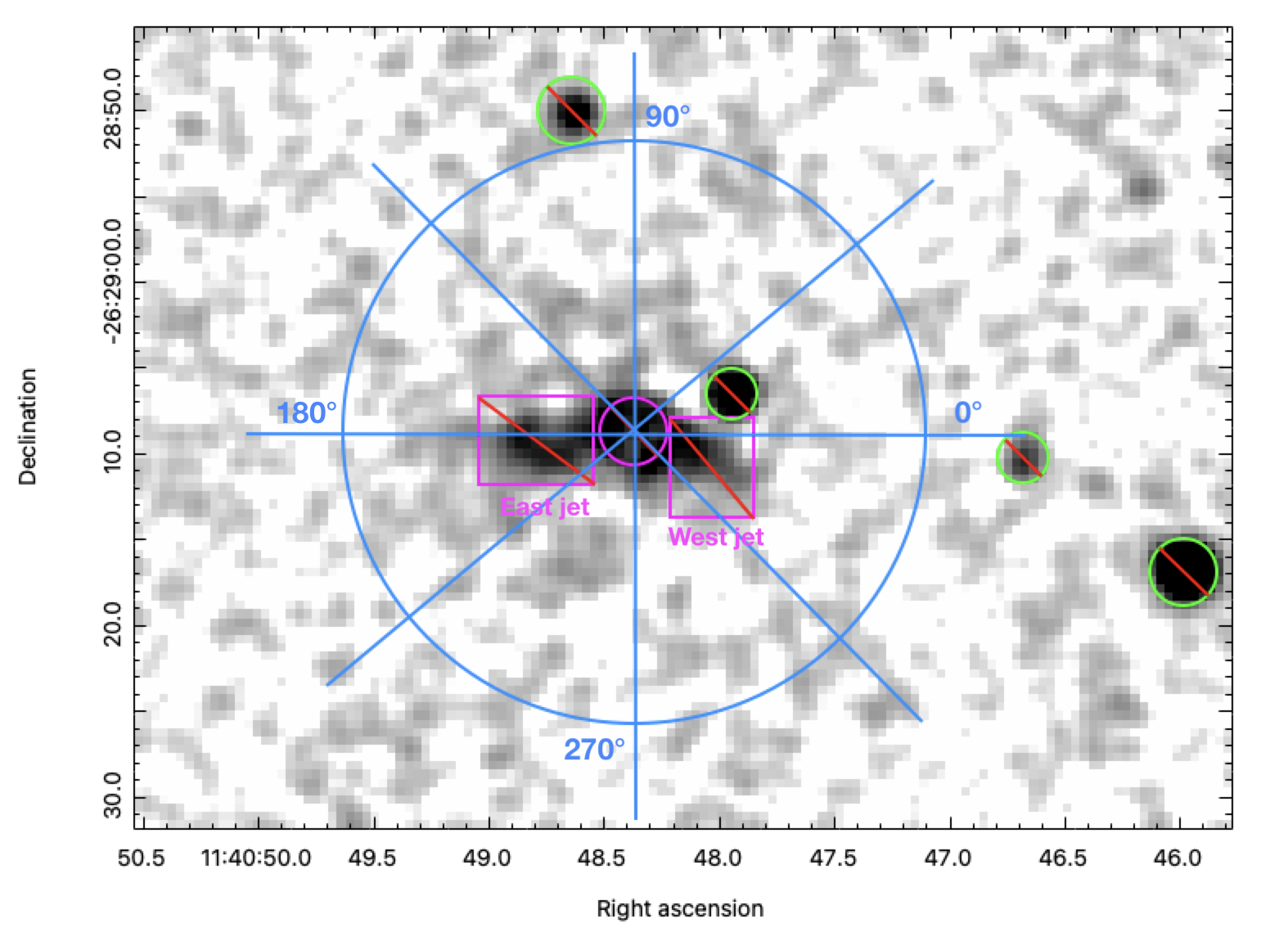
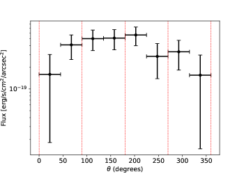
3.2 Azimuthal fluctuations

The previous measurement of the surface brightness distribution relies on two assumptions that are usually reasonable in the context of virialized massive halos: a center that is coincident with the central galaxy and a spherically symmetric distribution. Here, instead, we explore the presence of azimuthal fluctuations. To do so, first we considered eight different wedges with a step of 45 degrees (as shown in the left panel of Figure 2), extending up to a distance of 17 arcsec from the central AGN and excluding the central 2 arcsec and the jet regions. The average surface brightness in each wedge as a function of the position angle is shown in the right panel of Figure 2. We find that the azimuthal fluctuations of the average surface brightness in the wedges are consistent with isotropy. If we fit the points shown in the right panel of Figure 2 with a constant surface brightness as a function of the azimuthal angle, we find a reduced value, $\chi^{2}=1.1,$ with 7 d.o.f. To explore the effect of the wedge width, we repeated the measurement using 12 wedges with a step of 30 degrees. In this case, we obtained a reduced $\chi^{2}=1.18$ for 11 d.o.f. by assuming a constant surface brightness as a function of the azimuthal angle. This slight increase of the reduced $\chi^{2}$ is mostly due to a depression visible at $\sim 250$ degrees. This may point towards an actual decrease in the ICM surface brightness in this sector.

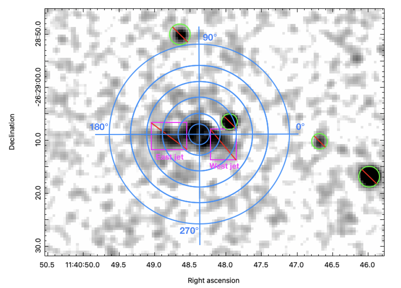
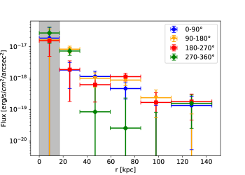
To further investigate the presence of azimuthal changes in the surface brightness distribution, we considered four quadrants (0-90, 90-180. 180-270, 270-360 degrees) and extracted the surface-brightness profile from circular concentric regions at a distance of 2, 4, 7, 10, 13, and 17 arcsec from the central source (see Figure 3, left panel). The four surface brightness profiles obtained are shown in Figure 3 (right panel), where a different color and symbol is associated with a different quadrant. We see a drop in the south-west quadrant in at least two bins, but with a statistical significance lower than 2 $\sigma$.

Overall, we conclude that the morphology of the X-ray emission can be reasonably approximated with a spherically symmetric surface brightness distribution centered on the AGN. Nevertheless, we also find hints of a departure from symmetry in the form of a depression of about an order of magnitude in the same quadrant where we find the western jet. Clearly, it is not possible to associate this depression to the effect of the jet, however, we argue that this feature may be associated with a cavity carved by the jet into the proto-ICM. Alternatively, this can also be a feature associated with the disturbed dynamics of the halo, or with the chaotic turbulent eddies which generate both compressions and depressions in the ICM (see X-ray maps in Gaspari et al., 2017). To further test these results, we explore the morphology of the SZ signal in the next section.

Figure 3: AGN-subtracted soft band image of the Spiderweb protocluster (left). The blue concentric circles, which correspond to 2, 4, 7, 10, 13, and 17 arcsec, and the blue lines separate the quadrants within which we derived the surface brightness as a function of the angle. Magenta squares represent the eastern and western jet excluded regions, while the green circles represent the excluded unresolved sources in the field of view. Surface-brightness profiles as a function of the distance from the central radio source (right). The grey-shaded area represents the surface brightness values parametrized with $n_{d}$.

4 SZ and X-ray combined analysis of the proto-ICM distribution

In the sections above, we describe how the X-ray surface brightness distribution of the proto-ICM in the Spiderweb protocluster reveals a depression in the south-west quadrant. Therefore, we would expect to find that the centroid of the X-ray emission is not centered on the radio galaxy, but is shifted towards the east. To quantify this shift, we analyzed the Chandra X-ray images with the Sherpa software in ciao.

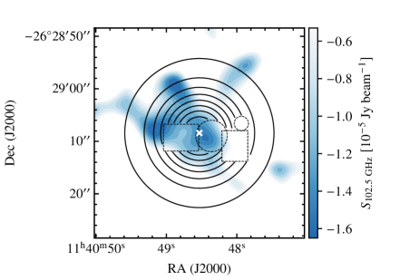
We considered the AGN-subtracted Chandra X-ray image in the soft band. However, here we mask a larger portion of the central region, removing a circle of 3 arcsec centered on the AGN. In this way, we removed the spike in the surface brightness distribution that we tentatively identified as a cool core (see Molendi & Pizzolato, 2001), which is further analyzed in the sections below. Then, we fit the surface brightness distribution with a single two-dimensional (2D) beta model plus background in order to find the X-ray centroid of the emission. As we can see from Figure 4, the X-ray emission centroid (white cross) is shifted towards the east by $\sim 2.3$ arcsec ($\sim 20$ kpc) with an uncertainty of $\sim 0.6$ arcsec.

Consistently with the findings of Di Mascolo et al. (2023), the pressure distribution of the proto-ICM electrons was instead reconstructed by means of a Bayesian forward modeling of the raw $uv$-plane interferometric data from Band 3 and 4 ALMA+ACA observations (Section 2.2). Briefly, the SZ distribution is obtained as the line-of-sight integral of a generalized Navarro-Frenk-White (NFW, Nagai et al., 2007) pressure distribution, with scaling parameters and radial slopes fixed to match specific formulations from the literature. In particular, we considered the full set of pressure models employed in Di Mascolo et al. (2023). An overview of the pressure model details can be found in Appendix A. For consistency with the X-ray analysis discussed above, we did, however, fix the centroid position of the SZ model component to match the one derived by modeling the soft-band X-ray surface brightness distribution. To fully account for the cross-contamination between the SZ signal and the extended emission from the Spiderweb radio galaxy, we inferred the SZ component jointly with the radio galaxy model, defined by the optimal, ordered set of point-like components, as in Di Mascolo et al. (2023). We also consistently imposed an upper threshold of $65\leavevmode\nobreak\ \mathrm{k\lambda}$ to the analysed visibilities to make the extended radio galaxy unresolved in the direction orthogonal to the jet axis. The posterior exploration was performed using the nested sampling algorithm (Skilling, 2004; Ashton et al., 2022), as implemented in the dynesty package (Speagle, 2020; Koposov et al., 2022).

Figure 4: Adapted from Di Mascolo et al. (2023): Contours from the SZ surface brightness map from a combined ALMA+ACA image (blue). The contours are set arbitrarily to optimally emphasise the bulk SZ signal. The black solid contours represent the model obtained with the single two-dimensional beta model fitting on Chandra AGN-subtracted X-ray image in the soft band, while the dotted circles and dotted squares represent the regions excluded in the analysis, namely, the eastern and western jets, central AGN, and an unresolved source. The white cross represents the X-ray emission centroid.

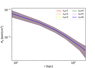
Despite the centroid assumption introduced above, the parameters for each of the reconstructed models are found to be statistically consistent with the ones reported in Di Mascolo et al. (2023), whereby the SZ shift with respect to the central AGN is 6.2 $\pm$ 1.3 arcsec. In this regard, we note that we observe a systematic reduction of the mass estimates, but they fall well within the respective statistical uncertainties, providing support to the robustness of the derived mass parameters (for details on the inferred models we refer to Appendix A, the corresponding Table 6 and also to Di Mascolo et al., 2023). In Figure 5 we show the pressure model obtained by means of Bayesian Model Averaging (BMA; Hoeting et al. 1999, Fragoso et al. 2018) applied to the different flavours of pressure profiles inferred with our analysis. Hereafter, we refer to the BMA model as the reference profile for the present study and we propagate the variance between the various pressure models in the marginalized posterior distribution.

Figure 5: Best-fit pressure profile obtained from SZ signal by marginalizing over the different gNFW models using a BMA technique. The solid lines denotes the median pressure profile, while the shaded regions mark the 68% credible interval on the posterior BMA model. We use different colors for different $n_{d}$, but we can see the pressure profile is not affected by this parametrization.

The low significance of both the SZ signal and the X-ray emission from the proto-ICM inevitably limits the possibility of performing a detailed morphological comparison. However, as already hinted at in Di Mascolo et al. (2023), we observe a marginal agreement between the bulk distribution of the proto-ICM inferred from the SZ signal and from the X-ray diffuse emission beyond 3 arcsec from the AGN (see Figure 4). This result provides a robust and straightforward confirmation of the global morphological picture obtained in both observational windows, confirming a substantial asymmetry consisting in a shift of the bulk of the ICM toward the east with respect to the Spiderweb galaxy. Alternatively, we may have identified a depression (tentatively a cavity, given the directional correspondence with the western radio jet) in the south-west quadrant. Unfortunately, we are not able to provide further constraints on the nature of the asymmetry in the proto-ICM with current data. As previously mentioned, we may interpret our result on the off-centered distribution of the ICM as a sign of the dynamical state remaining far from equilibrium or, alternatively, of ongoing radio-mode feedback. Both scenarios are further discussed in Section 6. Henceforth, we focus on the spherical approximation, to derive physical properties of the proto-ICM.

5 Thermodynamic properties

In this section, we analyze the thermodynamic properties of the proto-ICM in the halo of the Spiderweb Galaxy.

Table 1: Parameters and derived quantities of the beta model fit.

$n_{d}$	$r_{c}$	$S_{0}$	$n_{e0}$
	[arcsec]	[$10^{-17}$$erg/s/cm^{2}/arcsec^{2}]$	[$cm^{-3}]$
1	2.75$\pm$0.18	1.33$\pm$0.19	0.132$\pm$0.011
2	2.58$\pm$0.16	1.55$\pm$0.21	0.143$\pm$0.011
3	2.42$\pm$0.14	1.81$\pm$0.24	0.156$\pm$0.012
4	2.25$\pm$0.13	2.16$\pm$0.28	0.172$\pm$0.012
5	2.09$\pm$0.11	2.57$\pm$0.32	0.189$\pm$0.013
6	1.92$\pm$0.10	3.19$\pm$0.40	0.213$\pm$0.015

5.1 ICM density profile

According to the standard $\beta$-model (King, 1966; Cavaliere & Fusco-Femiano, 1976) the ICM is assumed to be an isothermal plasma in equilibrium with the galaxies in the same potential. Assuming that the galaxy distribution can be approximated as $\rho_{gal}(r)=\rho_{gal0}[1+(r/r_{c})^{2}]^{-3/2}$ (Cavaliere & Fusco-Femiano, 1978), the gas density, $n_{gas}$, can be written as:

$$n_{gas}(r)=n_{gas0}\biggr{[}1+\biggr{(}\frac{r}{r_{c}}\biggr{)}^{2}\biggr{]}^{-3\beta/2}\,,$$ (2)

where $r_{c}$ is the core radius and $\beta=\mu m_{p}\sigma_{r}^{2}/kT_{g}$ (with $\mu$-mean molecular weight, $m_{p}$-proton mass, $T_{g}$-gas temperature and $\sigma_{r}$-one-dimensional velocity dispersion). Consistently with Equation 2, the X-ray surface brightness profile at a projected core radius, $r,$ is expressed as:

$$S(r)=S_{0}\biggr{[}1+\biggr{(}\frac{r}{r_{c}}\biggr{)}^{2}\biggr{]}^{-3\beta+1/2}\,.$$ (3)

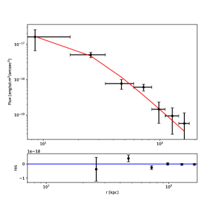
Typically, a value of $\beta\sim 0.66$ is a good, physically motivated approximation to describe the X-ray surface brightness and density profile in galaxy clusters (Cavaliere & Fusco-Femiano, 1976, 1978). The $\beta$ model is characterized by three parameters (normalization, core radius, and external slope). Measurements of the three offer a complete meaningful description of a spherically symmetric, self-gravitating halo. However, due to the well known degeneracy between $r_{c}$ and $\beta$, these two parameters may be simultaneously constrained only when the surface brightness can be probed over a broad range of radii from $r<<r_{c}$ to $r>>r_{c}$. In our case, given the low signal from the proto-ICM in the Spiderweb protocluster, we are limited only to the central regions, at the point where we can approximate the proto-ICM distribution with a constant density, as we did in Tozzi et al. (2022a). For the purpose of the analysis in this paper, to characterize the Spiderweb proto-ICM we fix $\beta=2/3$. The center of the $\beta$ model is fixed to the AGN coordinates and, therefore, it does not imply any additional free parameters. First, we fit the surface brightness profile, obtaining the values of $S_{0}$ and $r_{c}$ for different $n_{d}$ values reported in Table 1. The best-fit model for $n_{d}=4$ is shown in Figure 6. Error bars (at 1$\sigma$ confidence level) on the best-fit parameters were obtained by fixing alternatively the $r_{c}$ and $S_{0}$ parameters to their best-fit values. This was repeated for different values of $n_{d}$.

Figure 6: Best-fit of the surface brightness profile in the soft band for $n_{d}$=4 as a function of the distance from the AGN, shown as the red solid line, considering the extraction from the annular regions in Figure 1 (top panel). The X-ray surface brightness is shown with solid dots and associated error bars. Data points are the same as in Figure 1. Fit residuals are given in the bottom panel.

Then, in order to obtain the 3D electron density profile, we calculated the values of $n_{e0}$ deprojecting the $\beta$-model, using Equations 3 and 2 and using the relation between the normalization of the global X-ray spectrum measured in Tozzi et al. (2022a) and the electron density profile $n_{e}(r)$:

$$norm=\frac{10^{-14}}{4\pi[D_{A}(1+z)]^{2}}\int n_{e}(r)n_{H}(r)dV,$$ (4)

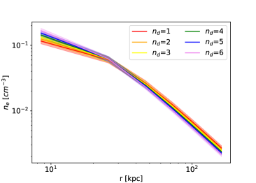
where $D_{A}$ is the angular diameter distance, while $n_{e}$ and $n_{H}$ are the 3D density profiles of electrons and hydrogen atoms, respectively. For simplicity, the volume $dV$ is simply the spherical volume included in the spectral extraction region of 12 arcsec. This implies that we ignore the contribution beyond this radius, which is, in fact, negligible (as shown in Figure 1) and has a minor impact on the normalization. The values of $n_{e0}$ are reported in Table 1. The deprojected electron density profile is shown in the left panel of Figure 7. As expected, the profile does not show features associated with spatial scales and it is similar to a power law. The central value is parametrized by the quantity $n_{d}$, while the best-fit profiles are affected overall by $n_{d}$ at a level lower than $5$%. Despite the fact that the central value ($r<2$ arcsec) is not constrained, the density profile does not show the inner flattening of a regular core; instead, it is growing roughly as a power law with slope $\sim 1.7$ towards low radii, as expected when a cool core is present.

Figure 7: Electron density as a function of the radius for different $n_{d}$ values (left). As we can see, the profiles differ significantly only in the central $\sim 2$ arcsec in which we apply the parametrization with $n_{d}$. Temperature profile as a function of the distance from the central radio source for different $n_{d}$ values (right). The solid black line represent the constant temperature value of the ICM found by Tozzi et al. (2022a), assuming an isothermal profile, while the shaded region mark the 1$\sigma$ errors associated with the temperature.

5.2 Pressure and temperature profiles

The inherent sensitivity limitation of the available X-ray data makes the measurement of a spatially resolved temperature profile almost impossible. An attempt to derive global temperature values from an X-ray spectral analysis in the annuli with radii of $2<r<7$ arcsec and $7<r<17$ arcsec has provided no indication of a difference in temperature in the two regions, with very loose contraints on both values. Therefore, the only reliable indication of the global (emission-weighted) temperature of the proto-ICM is that obtained in Tozzi et al. (2022a) from the X-ray spectrum, where we found $kT=2.0^{+0.7}_{-0.4}$ keV.

However, we can also constrain the temperature distribution in the Spiderweb proto-ICM by combining the SZ pressure profile with the X-ray surface brightness distribution. We remark that these two observables are completely independent and we do not make use of the information provided by the X-ray spectral analysis. In addition, despite the fact that the thermal SZ spectral distortion is potentially affected by the temperature through relativistic corrections, the impact with respect to ALMA Bands 3 and 4 is expected to result in a systematic shift of the order of $\lesssim 1.5\%$ of the total SZ signal (Mroczkowski et al., 2019), making this negligible compared to the intrinsic modeling and observational uncertainties (see Di Mascolo et al., 2023). Similarly, the deprojection of the surface brightness from soft-band X-ray data is only mildly affected by the assumed value of the proto-ICM temperature. On the other hand, the normalization of the SZ signal may be still affected by some systematics associated to the complex subtraction of the radio galaxy and the normalization of the surface brightness has some dependence on the unknown metallicity of the ICM. Both of these aspects should be taken into account when discussing our results.

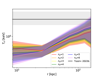
The radial profile of the temperature is directly obtained as the ratio of the pressure and electron density. In detail, the analytic estimate of the pressure distribution is obtained from the forward modeling of the ALMA data, while the binned density profile $n_{e}(r)$ is reconstructed from the soft-band X-ray surface brightness analysis (Section 5.1). Since the radial annuli are determined by the X-ray data, for consistency we post-processed the pressure profiles to estimate the $P_{e}(r)$ by marginalizing the values of the analytic realizations within each annulus (the resulting binned profiles are shown in Figure 5). Also in this case the profile can be roughly approximated with a power law, but with an average slope of $\sim 1,$ which is significantly flatter than the density profile. This directly implies a temperature gradient.

When simply assuming the ideal gas law, the average electron temperature within a given annulus is finally computed as the ratio $k_{B}T_{e}(r)=P_{e}(r)/n_{e}(r)$, as shown in the right panel of Figure 7. First, we notice a clear temperature gradient with value increasing from $\sim 0.6$ keV at $\sim 15$ kpc up to $\sim 1.8$ keV beyond 100 kpc. This result is interpreted as a very prominent cool core, showing the typical decrease by a factor of $\sim 3$ from the virial temperature reached at large radii and the emission-weighted temperature at the center. However, we do not see evidence for the expected flattening of the temperature profile with radius, probably because the X-ray signal disappear rapidly beyond 100 kpc (a distance still below the $r_{500}$ value of $(220\pm 30)$ kpc, as estimated in Tozzi et al. 2022a).

We note that the density-weighted temperature that we recovered from this profile, at radii larger than 2 arcsec, is $kT_{SZ,EW}=(0.7\pm 0.3)$ keV; this value is lower by a factor of $\sim 3$ with respect to that obtained in Tozzi et al. (2022a) with the X-ray spectral analysis ($kT=2.0^{+0.7}_{-0.4}$ keV, see the shaded area in Figure 7, right panel). A reason for this mismatch may be due to a residual contamination from non-thermal, diffuse emission in the region used to extract the X-ray spectrum of the ICM. Indeed, a small non-thermal contamination may result in a higher spectral temperature, while leaving the surface brightness practically unaffected. In addition, we also note that the ICM metallicity is practically unconstrained. The formal best-fit value is $\sim 0.25\,Z_{\odot}$ (in term of Anders & Grevesse, 1989), but this may be much lower than the actual value, considering that the bulk of the emission is coming from the core that is expected to be highly enriched by the ongoing SF. Assuming a value of $\sim 1\,Z_{\odot}$ ($\sim 2\,Z_{\odot}$) would reduce the spectral temperature by 3% (6%) and the normalization of the density profile by 15% (30%), corresponding to an increase of the density-weighted temperature by the same amount. This discussion suggests that the tension between the normalization of our temperature profile and the spectral value is significantly alleviated.

On the other hand, the normalization of the SZ signal may be underestimated compared to the actual pressure distribution due to the impact of the large-scale interferometric filtering. The overall sensitivity from the available ACA+ALMA observations is, in fact, driven by the ALMA compact configuration measurements, with a maximum recoverable scale of $\sim 26\leavevmode\nobreak\ \mathrm{arcsec}$ (corresponding to $216\leavevmode\nobreak\ \mathrm{kpc}$ at the protocluster redshift). This implies that any diffuse SZ component (generally expected in the case of morphologically disturbed and forming structures) will be inherently suppressed, thereby resulting in a systematic reduction of the amplitude of the inferred pressure model. Similarly, non-thermal contributions to the overall pressure budget due to merger-induced turbulent motion of the forming ICM, for instant, would cause the SZ signal to deviate from the hydrostatic equilibrium expectation (Bennett & Sijacki, 2022). Finally, as already mentioned in Di Mascolo et al. (2023), the complex dynamical state of the Spiderweb protocluster might introduce a significant kinematic component to the total SZ effect observed in the direction of the system. The limited spectral coverage at millimetre bands, however, does not allow for the different SZ contributions to be cleanly disentangled, resulting in a potential cross-contamination. In conclusion, the relatively low normalization of the temperature profile inferred from the SZ signal may be associated to a systematic effect in the ACA+ALMA data analysis.

To summarize, our results have revealed, for the first time, a clear temperature gradient associated with a cool core in a halo at $z>2$, showing that such structures form very rapidly as soon as the first cluster-sized halos start to collapse and virialize, around $z\sim 2.5$. The implication of these results will be discussed in the next sections.

5.3 Entropy and cooling time profile

In this section, we focus on the entropy and the cooling time profiles. If we assume the perfect gas law and consider a monatomic gas, the specific pseudo-entropy is given by:

$$K(r)\equiv kT(r)/n_{e}^{2/3}(r)=P_{e}(r)/n_{e}^{5/3}(r)\,,$$ (5)

where we combine the two independent measurements of $P_{e}(r)$ and $n_{e}(r)$.

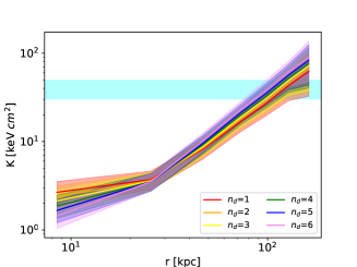
In virialized clusters, the entropy of the ICM is observed to follow a self-similar radial distribution with some deviation at the center, where it flattens (Ponman et al., 1999). However, cooling may re-establish a power law behavior in this region (see Voit & Bryan, 2001). Outside the core, the entropy profile shows the typical power law generated by gravitational processes (shocks and adiabatic compression, Tozzi & Norman, 2001) as also found in hydrodynamical simulations. For this reason, the entropy profile can be considered as the stratified thermal history of the ICM (Voit, 2005). The entropy profile obtained from the temperature and density profile according to Equation 5 is shown in the left panel of Figure 8. Apart from the poorly constrained first bin, which nevertheless always shows a slight flattening for any reasonable value of $n_{d}$, the entropy profile follows a power law with a slope of $\sim 1.1$, as expected for cool core clusters. If we consider the threshold between cool-core and non cool-core clusters, found to be between 30 and 50 keV cm² by Cavagnolo et al. (2009), the Spiderweb is classified as a strong cool-core cluster.

A very similar quantity is the cooling time, defined as the timescale in which the ICM entirely looses its internal energy through bremsstrahlung radiation. If we consider the ICM as a ionized gas in equilibrium, its internal energy is simply $(3/2)nkT$ and, therefore, the cooling time reads:

$$t_{\rm cool}\sim\frac{3}{2}\frac{nkT}{n_{e}n_{i}\Lambda(Z,T,n)}\,,$$ (6)

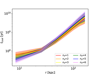
where $n_{e}$ and $n_{i}$ are the electron number density and the ion number density respectively, while $\Lambda(Z,T,n)$ is the cooling function which depends on the metallicity, $Z$, temperature, $T,$ and the number density (see, e.g., Donahue & Voit, 2022). At high temperatures, the cooling function is dominated by bremsstrahlung emission, while at low temperatures ($kT\leq 2$ keV), the cooling function is significantly affected by line emission from heavy ions. Again, we used the relation $kT(r)=P_{e}(r)/n_{e}(r)$ in Equation 6. The cooling time profile is shown in the right panel of Figure 8. We assumed the cooling function of Sutherland & Dopita (1993), with a metallicity of $Z=0.3\,Z_{\odot}$ in units of Anders & Grevesse (1989). However, we note that (as expected) the uncertainty in the ICM metallicity is only mildly affecting the cooling time since it is degenerate with the emission measure $\propto n_{e}^{2}$, as discussed in Section 5.2. We find that the average cooling time is lower than one Gyr within 70 kpc. Usually, one Gyr is a reference value used to define a cool core at $z\sim 0$ (see Hudson et al., 2010), and it should be significantly shorter at $z\sim 2.2$ when the age of the universe is 3 Gyr. More physically motivated definitions of core radii have been recently proposed (Wang et al., 2023). According to our results, the cooling time in the center can reach values below 0.1 Gyr, implying an unstable region where cooling can rapidly occur via multiphase gas condensation and a CCA mechanism, possibly triggered by mechanical feedback. In terms of CCA, we actually expect a higher frequency of triggering events at high-z, since diffuse baryons in the early universe are more often present in a multiphase stage and are more disturbed, even without in situ condensation and SMBH feedback (see Gaspari et al., 2012, 2013).

Figure 8: Entropy as a function of the distance from the central radio source for different values of $n_{d}$ (left). The cyan shaded area represents the threshold between cool core and non cool-core clusters found by Cavagnolo et al. (2009). According to this threshold, at radii $r<70$ kpc the Spiderweb can be classified as a strong cool-core cluster. Cooling time as a function of the distance from the central radio source for different values of $n_{d}$, assuming an ICM metallicity $Z=0.3\rm Z_{\odot}$ (right).

5.4 Total and ICM mass profile

Another quantity that we can immediately derive from the electron density and temperature profiles of the ICM is the total mass profile under the assumption of hydrostatic equilibrium, which is simply expressed as:

$$M_{\rm tot}(<r)=-r\frac{kT(r)}{\mu m_{p}G}\biggr{(}\frac{dlog(\rho_{g})}{dlog(r)}+\frac{dlog(kT)}{dlog(r)}\biggr{)},$$ (7)

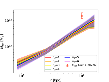
where $kT(r)$ is the temperature profile obtained in Section 5.2, $\rho_{g}$ is the gas density, $\mu$ is the mean molecular weight of the ICM, which is set to 0.6, and $m_{p}$ is the proton mass. The cumulative mass profile is shown in Figure 9 (left panel). The total mass computed at $r\sim 100$ kpc ($M_{\rm tot}=(0.60\pm 0.15)\times 10^{13}\,\rm M_{\odot}$) is lower than the value $M_{\rm tot}=(1.4\pm 0.3)\times 10^{13}\,\rm M_{\odot}$ obtained in Tozzi et al. (2022a), assuming a flat temperature profile. This discrepancy is entirely due to the difference between the X-ray spectral temperature derived in Tozzi et al. (2022a) and the temperature measured in this work.

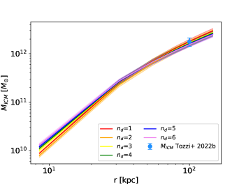
From the gas density $\rho_{g}(r)=n_{e}m_{p}A/Z$, where A and Z are the average nuclear charge and mass for the proto-ICM, we obtained the ICM cumulative mass profile, integrating over the volume:

$$M_{\textsc{icm}}=\int_{0}^{r}\rho_{g}(r)dV\,.$$ (8)

The cumulative ICM mass profile is shown in Figure 9 (right panel). We find that $M_{\textsc{icm}}=(1.64\pm 0.19)\times 10^{12}M_{\odot}$ within 100 kpc, in agreement with the average value of $(1.76\pm 0.30\pm 0.17)\times 10^{12}M_{\odot}$ (effectively an upper limit) found by Tozzi et al. (2022a), assuming a constant electron density distribution.

Figure 9: Total mass as a function of the radius for different $n_{d}$ values (left). The profiles differ mostly in the central $\sim 2$ arcsec. The red dot with errorbars represent the value of total mass at $r=100$ kpc based on the X-ray spectral temperature found by Tozzi et al. (2022a). ICM total mass as a function of the radius for different $n_{d}$ values (right). The blue dot with errorbars represents the value of ICM total mass at $r=100$ kpc found by Tozzi et al. (2022a).

6 Discussion

The analysis presented in this paper provides solid evidence for the presence of a cool core in the proto-ICM in the halo of the Spiderweb Galaxy and, at the same time, it offers some evidence to support a depression in the ICM distribution in the quadrant corresponding to the west radio jet. On the basis of the current data, we are not able to further constrain the properties of the proto-ICM, such as the actual MDR onto the BCG, or the energy budget of the feedback event – or even, alternatively, the dynamical state that may also be responsible for the asymmetry in the surface brightness distribution. We explore the possible implications of our findings below.

6.1 Estimate of the feedback energy budget

One of the results of this work is the presence of a possible depression in the X-ray surface brightness in the direction of the western jet, suggesting that the mechanical power of the central AGN may inflate a bubble of relativistic plasma in the ICM. For Fanaroff-Riley (FR) I radio sources in the Local Universe, the buoyancy arguments are often used to estimate the power that drives the expansion of the bubble (Gull & Northover 1973, Churazov et al. 2000; see also Fabian 2012 and Hlavacek-Larrondo et al. 2022 for reviews). Such estimates assume that during the subsonic expansion of the bubbles, buoyancy will eventually take over and drive the bubble up faster. For the subsonic expansion, most of the mechanical power of the outflow, $L_{m}$, goes into the enthalpy of the expanding bubble, according to the relation

$$L_{m}\times t\approx\frac{\gamma}{\gamma-1}PV=\frac{\gamma}{\gamma-1}P\frac{4}{3}\pi r_{b}^{3},$$ (9)

where $t$ is the age of the bubble, $P$ is the ICM pressure, $V$ is the volume of a spherical bubble with radius, $r_{b}$, and $\gamma$ is the adiabatic index of the gas inside the bubble ($\gamma=4/3$ for relativistic plasma). The corresponding expansion velocity of the bubble can be approximated as:

$$v_{\rm exp}=\frac{dr_{b}}{dt}\sim\frac{1}{3}\frac{r_{b}}{t}.$$ (10)

On the other hand, the terminal velocity of a steadily rising low-density bubble is set by the balance of the buoyancy force, $F_{b}=\frac{4}{3}\pi r_{b}^{3}\rho g$, and the drag force from the ICM acting on the bubble, $F_{d}=C_{d}\frac{1}{2}\pi\rho r_{b}^{2}v_{\rm rise}^{2}$. Here, $\rho$ is the mass density of the ICM, $g$ is the gravitational acceleration in the cluster potential well, and $C_{d}$ is the drag coefficient. For a subsonic spherical bubble in an incompressible fluid with a large Reynolds number, $C_{d}\sim 0.5$; while for flattened structures, it can be even greater (e.g., Zhang et al., 2018). Thus, the balance $F_{b}=F_{d}$ implies

$$v_{\rm rise}=\left(\frac{1}{C_{d}}\frac{8}{3}r_{b}g\right)^{1/2}=\left(\frac{1}{C_{d}}\frac{8}{3}\frac{r_{b}}{R}\right)^{1/2}v_{c},$$ (11)

where we express the gravitational acceleration at distance, $R,$ from the center of the cluster in terms of the circular velocity as $g=v_{c}^{2}/R$. Formally, this expression is valid as long as $r_{b}$ is much lower than the pressure scale height of the atmosphere. Once $v_{\rm rise}$ is larger than $v_{\rm exp}$, the buoyancy force deforms the bubble and moves it up in the cluster atmosphere. Requiring $v_{\rm rise}\approx v_{\rm exp}$ and solving for $t$ yields a lower limit on the mechanical power

$$L_{m}\gtrsim 3\frac{\gamma}{\gamma-1}P\frac{4}{3}\pi r_{b}^{2}\left(\frac{1}{C_{d}}\frac{8}{3}\frac{r_{b}}{R}\right)^{1/2}v_{c}.$$ (12)

This corresponds to the approach used in Churazov et al. (2000) for the Perseus cluster. There, an additional explicit assumption was made that for Perseus (and many other FR I sources) $r_{b}\sim R$ and, therefore, the term $\left(r_{b}/R\right)^{1/2}$ can be omitted. Here, we relax this assumption and use the values for R and $r_{b}$ that we derived from our data. Adopting $R=60\,{\rm kpc}$, $r_{b}=11\,{\rm kpc}$, $P(R)=5\times 10^{-11}\,{\rm erg\,cm^{-3}}$, $\gamma=4/3$, $C_{d}=0.75$, and $v_{c}=700\,{\rm km\,s^{-1}}$ we obtained the estimate:

$$L_{m}\gtrsim 10^{44}\,{\rm erg\,s^{-1}}.$$ (13)

Various other variants of the mechanical power estimate used in the literature are compiled in Bîrzan et al. (2004). They are also based on Eq. (9), namely, $L_{m}=\frac{\gamma}{\gamma-1}PV/t$, where for the value of $t$, the following alternatives are considered:

(i) the sound crossing time from the cluster core to the bubble

$$t_{cs}=\frac{R}{c_{s}},$$ (14)

where $c_{s}=\sqrt{\gamma_{g}\frac{kT}{\mu m_{p}}}$ is the sound speed in the thermal gas (ICM), $\gamma_{g}=5/3$, $kT=2\,{\rm keV}$, and $\mu=0.6$.

(ii) The buoyant rise time to the current position of the bubble with the terminal velocity

$$t_{\rm buoy}=\frac{R}{v_{\rm rise}},$$ (15)

which is similar to what we previously estimated (see Eqs.  10 and 11), but with a different normalization, and with $R$ replaced with $r_{b}$.

(iii) The refill time is:

$$t_{\rm refill}=2\sqrt{\frac{r}{g}}=2\frac{\sqrt{rR}}{v_{c}},$$ (16)

corresponding to the time required by a fluid element to cross the bubble’s diameter starting with zero velocity and constant acceleration, $g$.

Using the parameters we measured for the halo of the Spiderweb Galaxy, we obtained timescales of 80, 100, and 70 Myr for Eqs. 14, 15, and 16, respectively. This corresponds to a mechanical power of the order of $L_{m}\sim 10^{43}\,{\rm erg\,s^{-1}}$ or larger. Combining this outcome with the result of Eq. 13, we conclude that the AGN mechanical power is in the range of $\sim 10^{43}-10^{44}\,{\rm erg\,s^{-1}}$. This range of values is at the bottom of the distribution found by Hlavacek-Larrondo et al. (2015) in a sample of massive clusters out to $z\sim 0.7$. More precise measurements of cavity power in a sizeable sample of high-z clusters and protoclusters are needed to constrain the evolution of the average feedback power from BCGs. This is a clear science goal for future, high-resolution X-ray missions.

We note that this estimate relies on the assumption that pressure inside the bubbles is comparable to the ICM pressure, so that the expansion of the bubble is subsonic and the contribution of the kinetic energy of the expanding shells around the bubbles can be ignored. In fact, the estimated non-thermal pressure in some regions of the jets is $P_{nt}\sim 10^{-9}\,{\rm dyne\,cm^{-2}}$. This is an order of magnitude larger than the average ICM thermal pressure, estimated as $P_{ICM}\sim 5\times 10^{-11}\,{\rm dyne\,cm^{-2}}$ (Carilli et al., 2022). If $P_{nt}$ is the actual pressure inside the cavities, then the energy deposited in the ICM will be higher than the previous estimates, while the age estimates will be correspondingly lower (see the value $t\sim 3\times 10^{7}\,{\rm yr}$ obtained in Carilli et al. 2022). A much higher angular resolution would be needed to better characterizes the energy injection rate, by resolving the fine structure of the jets. In particular, the heads of the jets can propagate supersonically (e.g., Blandford & Rees, 1974; Begelman et al., 1984) due to the momentum of a collimated flow, differently from the expansion of a cocoon. As noted by Carilli et al. (2022), a part of the problem is that the Spiderweb Galaxy is a hybrid morphology radio source featuring a combination of FR I and FR II properties.

To summarize, despite the large uncertainties, if we interpret the surface brightness depression as a cavity in the ICM carved by the jets, we obtain a result that states that the power of the mechanical feedback from the radio galaxy is comparable or larger than the total rest-frame 0.5-10 keV luminosity of the ICM, observed to be $2\pm 0.5\times 10^{44}\,{\rm erg\,s^{-1}}$ (Tozzi et al., 2022a). This implies that the ongoing feedback is sufficient to compensate for ICM cooling losses. Clearly, since there is no information on the time span over which the feedback is acting, it is not possible to infer whether the cooling is already halted or, instead, whether cooling is steadily occurring while the feedback just kicked in. We note that stopping the cooling is completely extremely difficult, as during the self-regulated cycle, the feeding flow usually occurs perpendicular to the feedback jets (see maps in Gaspari et al., 2012).

6.2 The Spiderweb: A possible cool-core cluster in the making

There are no sources at low redshift that can be directly compared to the central halo of the Spiderweb protocluster. In this work, we find that the electron density shows a very steep profile that may reach $n_{e}\sim 10^{-1}$ $cm^{-3}$ in the central 10 kpc. In addition, we measure a very significant temperature gradient ranging from $kT\sim 0.6$ keV in the central 10 kpc to $\sim 2$ keV, clearly showing the presence of a strong cool core for the first time at $z>2$. These high density and low temperature values combined contribute to an extremely short cooling time in the central regions, possibly lower than $t_{\rm cool}\sim 0.1$ Gyr. The main question here is whether the presence of a strong cool core is the rule for massive virialized halos at $z>2$ or whether it is just a rare occurrence. Another key question is whether such high-redshift cool cores do host cooling flows with significant MDRs, which is at variance with cool cores in clusters at $z<1.5,$ where the cooling flows are generally quenched.

We can address this last point by deriving the MDR in the case of a steady-state, isobaric cooling flow (Fabian, 1994). We recall that this is the so-called ”classical cooling rate,” which is known to overestimate the actual MDR upper limits inferred in massive clusters from X-ray spectral analysis by10 to 100 times. The advantage of assuming the classic isobaric cooling flow model is that the luminosity emitted in any temperature range $dT$ can be immediately written as:

$$dL_{x}=\frac{5}{2}\frac{\dot{M}}{\mu m_{p}}k_{B}dT,$$ (17)

where $\dot{M}$ is the MDR, $\mu$ is the mean atomic mass, $m_{p}$ is the proton mass, and $k_{B}$ is the Boltzmann constant (Sarazin, 1988; Peterson & Fabian, 2006). To obtain the MDR, we calculated the X-ray luminosity in the soft band for the central $\sim 3$ arcsec (in which the cool core resides) as a function of the parameter, $n_{d}$. Accordingly, we get MDR values ranging between $\sim$ 250 $M_{\odot}/yr$ and $\sim$ 1000 $M_{\odot}/yr$, depending on the value of $n_{d}$. For $n_{d}=4$, which is the value that parameterizes the presence of a cool core, we get MDR$\sim 760\,\rm M_{\odot}$/yr. This value is close to the SFR values of $1390\pm 150\,\,\rm M_{\odot}$/yr (Seymour et al., 2012) or $1150^{+1150}_{-580}\,\rm M_{\odot}$/yr (Rawlings et al., 2013) found using IR observations, implying that a substantial fraction of the obscured SF may be sustained by gas cooling directly out of the hot ICM halo. Despite the fact that this is just a consistency argument and there are no additional proofs for the presence of a cooling flow in the ICM, it is worth considering this scenario in view of the potentially very young age of the cool-core/radio galaxy system in the Spiderweb protocluster. According to this scenario, the situation would be drastically different from that in clusters at $z<1.5$, where the secular evolution of the BCG regulates the ICM cooling and the residual SFR values observed in the BCG are typically more than one order of magnitude lower than the upper limits to the MDR measured in cool cores (see Molendi et al., 2016) .

6.3 Considering a possible high baryon fraction

Clusters and protoclusters are the most massive objects for which we can measure the baryonic mass (dominated by the ICM) and the total gravitating mass. Therefore, we can estimate the baryon fraction as the ratio of the ICM mass to the total cluster or protocluster mass. The baryon fraction we measure in this work at $r=100$ kpc is $f_{B}=0.33\pm 0.08$, about twice the value $f_{B}=0.16\pm 0.04$ found in Tozzi et al. (2022a). Therefore, we find a discrepancy at a level that is lower than 2$\sigma$. This is not due to the measured ICM mass, whose values are consistent in Tozzi et al. (2022a) ($M_{ICM}=(1.76\pm 0.3\pm 0.17)\times 10^{12}\,M_{\odot}$) and in this work ($M_{ICM}=(1.64\pm 0.19)\times 10^{12}\,M_{\odot}$). In fact, the largest discrepancy with respect to our previous work is in the temperature and, hence, on the total mass measured at $100$ kpc. The total mass measured in Tozzi et al. (2022a) from X-ray spectroscopy is $M_{tot}=(1.4\pm 0.3)\times 10^{13}M_{\odot}$, while from the ratio of X-ray emission and SZ signal we obtain $M_{tot}=(0.60\pm 0.15)\times 10^{13}M_{\odot}$.

As we discuss in Sec. 5.2, an overestimation of the X-ray spectroscopic temperature may be ascribed to a residual contribution of non-thermal emission overlapped with what we consider thermal ICM emission. This unnoticed contribution may have a significant impact in the spectrum, while having just a minor effect on the surface brightness distribution. We also mentioned in Section 3, the possibility of an isotropic IC emission due to a (unlikely) precession of the radio jets. At the same time, systematics in the derivation of the SZ signal, may be the cause of the low temperature inferred from SZ, providing additional reasons to favor a total mass closer to the value of $M_{tot}=(1.4\pm 0.3)\times 10^{13}M_{\odot}$ measured in Tozzi et al. (2022a).

Nevertheless, we notice that both estimates of the baryon fraction are higher by a factor ranging from 2 to 5, than those measured in local clusters of comparable mass scale (see Gonzalez et al., 2013). Therefore, we argue that the observed proto-ICM may be in an overdense phase and it has not reached virial equilibrium, yet with the underlying dark matter halo. This may be due to an early phase of the gravitational collapse, or an inside-out shock heating of the diffuse baryons. As we know, in the same regions a significant amount of warm and cold baryons have been observed. Clearly, this is a highly speculative scenario, that should be tested by observing other proto-ICM cores and with deeper X-ray data, a task that became almost impossible due to the dramatic loss of sensitivity of Chandra. Given the uncertain significance of this tension, we did not further explore this aspect within our data set.

6.4 Weighing the potential commonality of the Spiderweb protocluster

If we focus on the association of an extreme starburst BCG with a cool core, the Spiderweb Galaxy has very few comparable sources in the $0<z<1.5$ range. So far, we know that in this redshift range, almost all the relaxed and virialized clusters have a cool core but no (or residual) cooling flows, as a result of the secular evolution of the nuclear activity in BCGs, and of the high duty cycle of radio AGN in cluster cores. Nevertheless, we know a few exceptions to this scenario, the most relevant case being the Phoenix cluster at z$\sim$0.6, that is classified as a rapidly evolving cool core cluster (McDonald et al., 2013; Tozzi et al., 2015; McDonald et al., 2019; Kitayama et al., 2020). The Phoenix cluster has a much higher mass scale with respect to the Spiderweb protocluster, and, most importantly, it is observed at a cosmic epoch 5 Gyr after the Spiderweb. As such, the Phoenix must have experienced several feedback events that should have quenched the potentially massive cooling flows. However, current estimates of the MDR in the Phoenix amount to $350^{+250}_{-200}\,\rm M_{\odot}$/yr below 2 keV (Pinto et al., 2018), comparable to the SFR in the BCG. In the case of the Phoenix, the AGN activity may be overcome by a high accretion rate due to the large halo mass and an undisturbed dynamical evolution, leading to a cool core stronger than usual. An alternative explanation is provided by a young stage of the feedback process, a situation that is clearly preferred in the Spiderweb, due to the much younger cosmic epoch. A possible way out is to reconstruct the feedback history as recorded in the ICM, by identifying old cavities still buoyantly raising in the outskirts, where the surface brightness of the ICM is much lower and the surface brightness contrast of a cavity well below the sensitivity of current facilities. Another strategy to approach this issue is the statistical study of the halo population, searching for unbalanced cool cores at different cosmic epochs.

While the occurrence of strong cool cores in halos at $z>2$ is unknown and it will be explored only with future X-ray and optical/IR/radio telescopes, we may argue that any massive cluster at $z<1$ comparable to the Phoenix should be easily identified and characterized by current X-ray facilities. While awaiting the results from the eROSITA survey, we may mention only three other cool core clusters at $z<1$ that may be compared to the Phoenix: ZwCl235 (z$\sim$0.08, Ubertosi et al., 2023, which also has a pair of cavities excavated by the central galaxy), RXC J2014.8-2430 (z=0.15, Mroczkowski et al., 2022), and RX J1720.1+2638 (z=0.16, Perrott et al., 2023). At $z>1$, we may include two dynamically relaxed cool core clusters: SPT-CL J0607-4448 ($z=1.4$, Masterson et al., 2023) and SPT-CL J2215-3537 ($z=1.16$, Calzadilla et al., 2023). We argue that pushing the X-ray spectral analysis to the limits of current facilities in the Phoenix analogs at $z<1.5$ may shed light on the mechanism regulating the quenching and onset of cooling flows in cool cores, to be compared to what happens in younger halos at $z>2$.

Very little is known of the behavior of diffuse baryons in protoclusters. Both the presence of proto-ICM and the occurrence of significant cooling events from the hot component is clearly expected to be limited to the most massive halos within the protoclusters themselves that, by definition, have an average overdensity about one order of magnitude lower than in virialized halos. Still, cooling flows may form at any time, due to the short time scales that may prevent feedback and the larger disturbances, as compared with the low-z counterparts. We suggest, therefore, that the phase observed in the Spiderweb protocluster may not be an evolved cool core like the one observed in virialized clusters but, rather, a precursor phase associated with the presence of the radio galaxy.

So far, the characterization of proto-ICM at $z>2$ has been extremely challenging, despite the fact that most of the protocluster have been identified thanks to the presence of a high redshift radio galaxy placed within an overdensity of galaxies. Venemans et al. (2007) found that $\sim$ 75$\%$ of radio galaxies are located within protoclusters traced by Ly$\alpha$ emitters (LAEs), considering a sample of nine radio galaxies (see also Matsuda et al., 2009; Galametz et al., 2012; Wylezalek et al., 2013). Nevertheless, due to the extreme faintness of the expected diffuse X-ray emission, a deep and systematic X-ray surveys of such galaxies has never been attempted. A first step may be obtained by the X-ray follow-up of high-z radio galaxies with the most peculiar radio morphologies, such as the presence of a simultaneous FRI and FRII jets type (Carilli et al., 2022). The first discoveries of these hybrid morphology radio sources date back to the work of Gopal-Krishna & Wiita (2000), up to the most recent work of Gopal-Krishna et al. (2023), with the discovery of radio galaxies 4C+63.07 at z$\sim$ 0.3 and J1136-0328 at z$\sim$0.8. At higher redshift, instead, we mention the radio source 4C65.15 at $z=1.63$ (Miller & Brandt, 2009), J1154+513 at $z=1.34$ and J1206+503 at $z=1.45$ (Stroe et al., 2022).

Alternatively, the presence of a protocluster may be obtained by the detection of LAE overdensity. Among the most promising sources, we take note of MRC 2104-242, which is a HzRG (z=2.49, Overzier et al., 2001) located within an overdensity of galaxies (about eight times the average field, Cooke et al., 2014) with typical SFR of $\sim 10-100\,\rm M_{\odot}/yr$ and masses in the range of $\sim 10^{10}-10^{11}\,\rm M_{\odot}$. In addition, it is embedded within a Ly$\alpha$ emitting halo that extends for $\sim$ 136 kpc, showing two large clumps and a very large velocity distribution ($\sim 1000-5000$ km/s, Overzier et al., 2001). We also mention the radio galaxy 4C-00.62 (Kajisawa et al., 2006) which is located at $z=2.53$ within the USS 1558-003 protocluster, with a LAE overdensity showing three prominent structures (Shimakawa et al., 2018).

At lower redshift, 7C 1756+6520 ($z=1.42$, Galametz et al., 2009, 2010) inhabits an environment very similar to the Spiderweb, with a prominent galaxy overdensity (among which 21 spectroscopically confirmed) with several AGN candidates. The protocluster found in the field of a quasar at z$\sim$6, SDSS J1030+0524 Gilli et al. (2019) hosts a radio galaxy surrounded by an overdensity of galaxies (11 spectroscopic members in a distance of $\sim$ 1.15 Mpc; D’Amato et al., 2020) with $SFR\sim 8-600\,\rm M_{\odot}/yr$. This structure seems far from being virialized but shows diffuse X-ray emission that can be at least partially associated with an expanding bubble of gas at temperature T$\sim$ 5 keV (Gilli et al., 2019). In this framework, the presence of promising targets coupled to the lack of a systematic approach and of a high-resolution, wide-angle X-ray survey, force us to conclude that the best effort at the moment is to develop a systematic approach with SZ observations and to exploit, at the same time, current X-ray facilities to push as deeply as possible on the best-candidate protoclusters identified so far.

7 Future perspectives

Our results demonstrate the central role of a sharp Chandra-like PSF for detailed analyses of the ICM properties of high-z protoclusters. The role of X-ray data with high-angular resolution will be key for the extension of this approach to a large sample of protoclusters. Currently, Chandra is the only facility that can provide data of the required quality. As a complementary tool, XMM-Newton can contribute with the characterization of the X-ray properties of high-z radio galaxies, but with a loose grasp on possible extended thermal emission on scales of $\sim 10$ arcsec. Therefore, the future of this science case heavily depends on the future of high-resolution X-ray astronomy, carried out with the advent of the next generation of X-ray satellites, such as AXIS (Mushotzky et al., 2019; Marchesi et al., 2020), the survey and time domain mission STAR-X (Zhang et al., 2022), Lynx (The Lynx Team, 2018), and Line Emission Mapper (LEM; Kraft et al., 2023). Thanks to a large field of view to increase the discovery space, a high resolution (in the range 0.5-3 arcsec) and a high effective area, particularly in the soft band, it will be possible to characterize the emission of the ICM at $z\sim 3$ and untangle this emission from the AGNs emission, to map density, temperature, and also non-thermal emission at physical scales below 5 kpc.

As already discussed in Section 1, the complementary and alternative way to study protoclusters and the formation, evolution and structure of the ICM, is provided by interferometers and single dish instruments from the ground. In the last decade, interferometers like ALMA and ACA have been able to observe the diffuse gas and confirm the membership in protoclusters at $z>2$ using molecular gas emission line such as CO lines. Unfortunately, current (sub-) millimeters interferometers do not allow us to explore significantly larger areas without being exceedingly time-consuming due to a small field of view. Also, they are only sensitive to emissions on scales inversely proportional to their baseline separations, making them insensitive to large-scale emission (the so-called “missing flux” problem). For these reasons they have extreme limitations for mapping the tenuous gas in protoclusters and the SZ effect on larger scales with a high angular resolution.

Recently, a promising improvement that has been made on ALMA is the introduction of Band 1 (35-50 GHz), which allows us to increase the maximum recoverable scale, making it easier to study the SZ signal from diffuse gas on larger scales. This will also allow us to provide unprecedented detailed analysis of the ICM and its thermodynamics and to detect substructures in protoclusters. Unfortunately, at this point interferometers are and will be mainly useful to focus on known targets for detailed follow-up studies, with very little room for the discovery of new targets. This situation leads to the problem of ”source starvation.”

Single-dish facilities, on the other hand, should allow us to map this emission with greater resolution and at higher sensitivities. One possible future single dish that would combine dish diameters and with a large field of view is AtLAST (Klaassen et al., 2020; Ramasawmy et al., 2022). Indeed, AtLAST’s key parameters include a 50 m aperture and a 2 deg field of view. It will be built in a location with excellent atmospheric transmission at millimeter/submillimeter wavelengths. Thus, the combination of arcsec-scale angular resolution with broad frequency coverage ($\approx$30-950 GHz) and multiple bands sampling the SZ effect spectrum, will allow us to study the hot ICM on larger scales, sample the resolved SZ effect across a wide range of redshifts and in different environments (from groups to clusters and protoclusters), detect dynamical effects on diffuse gas and explore variations in pressure and temperature profiles. Considering that both AtLAST and STAR-X may be operating in 2030, the perspective of having a systematic and statistically significant investigation of the proto-ICM in the range $2<z<3$ may become reality in less than ten years.

8 Conclusions

In this paper, we present a detailed analysis of the thermal diffuse emission of the proto-ICM detected in the halo of the Spiderweb Galaxy at $z=2.16$ within a radius of $\sim 150$ kpc. We simultaneously analyzed the deep X-ray data from Chandra and the SZ signal obtained with ALMA sub-millimeter data. Our results can be summarized as follows:

• Thanks to the Chandra X-ray data we find that the azimuthally averaged surface brightness is well characterized in the soft band, while the photometry in the hard band is consistent with no detectable signal. This confirms that the diffuse emission is consistent with being bremsstrahlung emission at $\sim 2$ keV or lower.

• We also find a mild evidence of asymmetry in the X-ray surface brightness, in the form of a depression in the sector corresponding to the direction of the western jet. This feature may be tentatively associated with a X-ray cavity carved into the hot baryons and filled with low-density relativistic plasma, which originated as a displacement of gas due to the radio jets. In this case, the estimated energy power of the associated feedback events is in the range $10^{43}-10^{44}$ erg/s, depending on the method used to estimate the mechanical power. Alternatively, the asymmetry may be due to the young dynamical status of the halo.

• From the 2D analysis of the X-ray data, we find that the bulk of the X-ray emission (excluding the central core within a radius of 3 arcsec) has the centroid located at a distance of $\sim 2.3$ arcsec from the AGN. This shift is along the same direction of the SZ effect offset (6.2 $\pm$ 1.3 arcsec) measured with ALMA.

• We combine the electron density profile from X-ray data and the pressure profile from the SZ effect to derive for the first time the temperature profile of the proto-ICM. We find a strong temperature gradient, corresponding to the increasing electron density profile towards the central AGN, revealing the presence of a strong cool core. This result is robust despite the $2\sigma$ disagreement at face value between the normalization of the temperature profile and the X-ray spectral, single temperature obtained in Tozzi et al. (2022a).

• From the temperature and electron density profiles, we obtain the total mass profile assuming hydrostatic equilibrium, as well as the ICM mass profile. We find a total mass value of $M_{\rm tot}(100kpc)=(0.60\pm 0.15)\times 10^{13}$$M_{\odot}$, a factor of 2 lower than the value measured in Tozzi et al. (2022a) assuming an isothermal ICM of $\sim 2$ keV. The ICM mass is measured to be $M_{\textsc{icm}}=(1.64\pm 0.19)\times 10^{12}\,\rm M_{\odot}$, in agreement with the upper limit of $(1.76\pm 0.30\pm 0.17)\times 10^{12}\,\rm M_{\odot}$ found by Tozzi et al. (2022a) using a constant density profile.

• Using the temperature and electron density profile, we obtain the entropy profile, that follows a power law as expected in cool cores. Correspondingly, the cooling time profile shows values lower than 1 Gyr below 70 kpc from the central AGN, possibly reaching values as low as 0.1 Gyr in the innermost 20 kpc, suggesting that the cooling may occur on a time scale shorter than the AGN duty cycle.

• We argue that, if the feedback is not effective yet in reheating the cooling ICM, a cooling flow may develop, with a MDR in the range 250-1000 $M_{\odot}/yr$, consistent with the SFR values found using IR observations, implying that a substantial fraction of the obscured SF may be sustained by gas cooling directly out of the hot ICM halo.

To summarize, for the first time we constrain the thermodynamic properties and the hot baryon circulation in the core of a protocluster at $z>2$, thanks to an unprecedented combination of deep, high-resolution Chandra X-ray data and SZ ALMA data. As expected, the first stages of formation of protoclusters are characterized by an extreme environment with energetic feedback events that may coexist for a relatively short time with massive cooling flows episodes. The systematic studies of proto-ICM halos in protoclusters may reveal a new, short and intense phase of heating and cooling, just before the BCG, its AGN activity and the ICM are driven into the secular evolution achieved when the feedback efficiently quench cooling flows, as commonly observed at $z<1.5$.

Appendix A Pressure models

To date, we continue to lack an exhaustive theoretical description of the expected distribution of the thermodynamic properties of the ICM forming within protocluster structures. To fully account for potential biases and variance introduced when forward modeling the proto-ICM thermodynamic profiles by means of models calibrated on low-redshift cluster samples, Di Mascolo et al. (2023) performed a comparative analysis of the SZ signal in the direction of the Spiderweb protocluster by means of different gNFW models from the literature, namely: the pressure profile derived by Arnaud et al. (2010), using both its universal formulation (A10 UP) and the one constrained on the subset of morphologically disturbed (A10 MD) clusters; the universal (M14 UP) and non-cool-core (M14 NCC) pressure profiles by McDonald et al. (2014); the median profiles derived from the simulated cluster set in Le Brun et al. (2015) and under different assumptions for the AGN contributions (L15 REF, L15 8.0, L15 8.5; we refer to Le Brun et al. 2014, 2015 for details on the physical prescriptions for the AGN-driven heating); the self-similar extended pressure model by Gupta et al. (2017).

In this work, we repeat the same analysis but fixing the coordinates of the SZ centroid to the one inferred from the X-ray analysis in Section 4. In such a way, the parameter set for each parameter reduces to the mass term only. A summary of the best-fit values of the virial mass $M_{500}$ for each pressure model is reported in Table 6.

Table 2: Comparison of the best-fit parameters for the different SZ models employed in the analysis.

	$M_{500}$	ref.
	[$10^{13}\leavevmode\nobreak\ \mathrm{M_{\odot}}$]
A10 UP	$2.47\begin{subarray}{c}+0.44\\ -0.54\end{subarray}$	Arnaud et al. 2010
A10 MD	$2.01\begin{subarray}{c}+0.39\\ -0.49\end{subarray}$	Arnaud et al. 2010
M14 UP	$2.82\begin{subarray}{c}+0.53\\ -0.65\end{subarray}$	McDonald et al. 2014
M14 NCC	$2.84\begin{subarray}{c}+0.53\\ -0.66\end{subarray}$	McDonald et al. 2014
L15 REF	$2.59\begin{subarray}{c}+0.42\\ -0.48\end{subarray}$	Le Brun et al. 2015
L15 8.0	$4.30\begin{subarray}{c}+0.55\\ -0.68\end{subarray}$	Le Brun et al. 2015
L15 8.5	$6.54\begin{subarray}{c}+0.78\\ -0.95\end{subarray}$	Le Brun et al. 2015
G17 EXT	$2.20\begin{subarray}{c}+0.39\\ -0.55\end{subarray}$	Gupta et al. 2017