Images of the Ultra-High Energy Cosmic Rays from Point Sources

Abstract

Our latest paper [1] investigates the effects of UHECR propagation in a turbulent intergalactic magnetic field in the small-angle scattering regime, specifically focusing on the non-trivial caustic-like pattern that arises with strong deviation from isotropy. In this paper, we explore the effect of the observer’s position on the measurement of source flux at a given distance. We examine three types of source locations, characterized by the density of cosmic rays from a given source at the observation point, which we call knots, filaments and voids. We also investigate the energy spectrum in these different cases and present simulated images of the source as it appears on the observer’s telescope after propagation in the combination of intergalactic and Galactic magnetic fields. We show that hot spots in the UHECR data can arrive due to combined distortions of source images on the intergalactic and Galactic magnetic fields. Also the fact that flux of most nearby sources is diluted in the voids affects source population studies.

I Introduction

Contrary to photons and neutrinos, Ultra-High Energy Cosmic Rays (UHECR) are charged particles and they are unavoidably deflected in the Galactic and intergalactic magnetic fields. Expected large number of UHECR sources in the Universe together with large deflections of UHECR from source positions prevents to do astronomy except for the highest energies $E>6\cdot 10^{19}$ eV, where the spectrum has cutoff due to interactions with Cosmic Microwave Background (CMB). This so called GZK cutoff was predicted by Greizen, Zatsepin and Kuzmin in 1966 [2, 3] and was observed 40 years later by HiRes experiment in 2007 [4] and later confirmed with large statistics by modern experiments Pierre Auger Observatory (Auger) [5] and Telescope Array (TA) [6]. Existence of GZK cutoff guarantees that UHECR with energies $E>6\cdot 10^{19}$ eV come from local Universe with significant contribution of sources located in nearby Large Scale Structures (LSS) with distance to our Milky Way galaxy $R<200$ Mpc. Since LSS at those distances is significantly non-uniform, this gives a hope to see individual UHECR sources. Astronomy with UHECR at the highest energies $E>6\cdot 10^{19}$ eV was one of the main motivations for the construction of Auger and TA experiments.

For cosmic ray protons deflection in the $B_{\mathrm{Gal}}\sim\mu$G Galactic magnetic field is only few degrees for $E>6\cdot 10^{19}$ eV depending on direction. Intergalactic magnetic fields order of $B_{\mathrm{IGMF}}\leq n$G are again not efficient to disturb UHECR proton directions from point sources. Thus one expect to see point or slightly extended sources of protons $E>6\cdot 10^{19}$ eV in UHECR data. However, even with large exposure Auger and TA have not found any signature of point sources. This observation is consistent with statement made by Auger that most of UHECR with $E>6\cdot 10^{19}$ eV are intermediate and heavy nuclei. In the case of heavy nuclei, the Galactic magnetic field disturbs and even washes out images of UHECR sources [7, 8].

After years of observation, Auger and TA see several anomalies in the sky that look like hot spots with a radius of 10-20 degrees. These hot spots can be images of nearby point sources, disturbed both in Galactic and extragalactic magnetic fields.

Previous studies have explored the effects of intergalactic magnetic fields on the trajectories of UHECRs. One such study, [9], investigated the Centaurus A UHECR excess and its potential connection to the local extragalactic magnetic field. This study shows that, assuming a proton composition, the strength of the extragalactic magnetic field should be at least 20 nG. The latter value is in conflict with existing observational constraints [10, 11, 12]. In present work we assume a high but realistic magnetic field strength.

Main goal of the present study is to show that the observed 10-20 degree radius hot spots in UHECR data can be signals from nearby point sources, disturbed both in Galactic and intergalactic magnetic field. In particular, we show examples of sources, which can explain TA hot spot. We show that caustic-like pattern of intergalactic magnetic field amplify small number of sources in filaments and knots and at the same time reduce contribution of most of nearby sources.

II Simulation

To obtain images and spectra of UHECR sources, we rely on numerical simulations of UHECR propagation. Our simulation procedure generally consists of two steps. In the first step, we propagate UHECRs in turbulent intergalactic magnetic fields, tracing their paths until they reach the edge of our galaxy. In the second step, we consider the effect of the galactic magnetic field and construct images at the Earth’s position.

For intergalactic propagation we use 3D Monte Carlo code CRbeam[14] which allows to take into account UHECR deflections in magnetic fields and interactions with CMB and EBL. The general setup of the these simulations is the same as in our previous paper [1]. The main difference is the possibility of emitting particles in the form of a jet with a given opening angle and axis direction (isotropic source is thus a special case with opening angle equals $\pi$). In all simulations we keep flat profile of the jet. Another important modification is that we catch particles when they hit a small spherical observer which represents our galaxy. The radius of observer was chosen to be 100, 200 or 1000 kpc, the last one for void cases. Once the particle hits the observer, we record its energy, momentum, and position on the sphere. We subsequently use this information to reconstruct the source image.

CRbeam represents turbulent magnetic field with Kolmogorov’s spectrum as a sum of plain waves with random directions and phases, following the method of [15]. The number density of waves is uniform in logarithmic scale by wavenumber. We fix the number of waves to be 463 with the largest eddy being 100 larger than the smallest. A smaller number of waves may lead to an unwanted effect when a wave with the longest wavelength dominates UHECR deflection. On the over hand, bigger number of waves increase calculation time. In our previous study [1], we carefully verified that existence of the caustic-like patterns in UHECR spacial distribution does not depend on either the method of generating the turbulent magnetic field or its spectrum. Therefore, we believe that our result are stable with respect to the technical parameters of the magnetic field generators such as number of modes and maximum and minimum scales of the spectrum. We keep the same random seed for magnetic field generation in all simulations within the paper and use OpenMP for multiprocessing acceleration.

The magnetic field strength was set to $B=1$ nG and correlation length $\lambda_{\mathrm{c}}=1$ Mpc. In most simulations, we propagate protons with an energy of $E=10$ EeV, but our results remain unchanged if one proportionally rescales the particle’s charge and energy.

The typical scale of distances we consider here is about tens of Mpc. Given the fact that the size of the observer is tens of kpc and protons have nonnegligible deflections in IGMF with $B\propto 1$ nG the problem of aiming at the observer arises. This is due to both a decrease in the angular size of the observer with distance and to the fact that statistically more often the observer finds himself in the region of space where the cosmic ray flux from point source is even lower than expected from standard inverse-square law [1]. This prompts the need of targeting algorithm.

Optimization of the targeting mechanism was studied earlier, for example in [16]. The authors used von Mises–Fisher distribution instead of simple cone jet and solve task for only one distance and energy. We reproduced this approach and modified it for our case to optimize the performace for our case.

Since we are examining the source images and flux excess/deficit at different distances or energies, we apply the following procedure for optimization of calculation time. First, we aim to observer from small distance $D_{\mathrm{1}}$ where deflection by magnetic field is negligible. After that we use the directions found on the preceding step at distance $D_{\mathrm{i}}$ for aiming on distance $D_{\mathrm{i+1}}>D_{\mathrm{i}}$ ($D_{\mathrm{i+1}}-D_{\mathrm{i}}\sim 0.5-2$ Mpc $\lesssim r_{\mathrm{g}}$ in our cases where $r_{\mathrm{g}}$ is gyroradius given by $r_{\mathrm{g}}=\frac{E}{\mid q\mid B}$).

Another simulation parameter – jet angle $\theta$ is chosen as previous minimal necessary jet angle multiplied by a constant factor. We have empirically seen that a value of $\sim 3$ for this factor allows to ensure that the most of the flux have not been missed. We obtain minimal necessary jet angle from the analysis of particle directions in CRbeam output files. For the first run we choose $\theta_{1}\sim\frac{\pi}{2}$ or $\theta_{1}\gtrsim\arctan(\frac{R_{\mathrm{obs}}}{D})$. If simulation has strong flux deficit, it is restarted with the wide angle of the jet $\theta\propto\sqrt{D\lambda_{\mathrm{c}}}/E$ (see [1]) to ensure that all particles which may reach the observed are included into emitted jet.

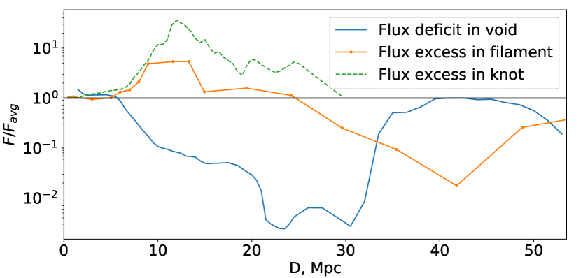
To estimate the simulation acceleration factor, let’s consider the Fig. 2. The flux can decrease by more than $\sim$100 times compared to the average at a distance of $\sim$20 Mpc, at this distance the observer occupies no more than $10^{-3}$ of the entire manifold of end particles coordinates. So, the probability of hitting an isotropically emitted particle is less than $10^{-5}$. Therefore, obtaining sufficient statistics would take a long time. Using the procedure explained above allows to direct particles into a cone with an angle of $\theta\sim 0.2$ radians and the geometric probability of hitting increases by about $2/(1-\cos(\theta))\sim 100$ times. So, the Fig. 4 have been simulated about 100 times faster than if the source was considered isotropic.

Finally we take into account deflections in galactic magnetic field and obtain images of the sources as seen by observer at Earth’s position inside the galaxy. We use galactic magnetic lenses provided by CRPropa3 [17, 18], which enables efficient utilization of backtracking simulations to consider galactic deflections in forward simulations of UHECRs. We adopt the JF12 model of galactic magnetic field with both coherent and turbulent components turned on [19, 20].

III Results

III.1 Observed fluxes

Figure 1: Probability of observer to be located in the region with flux higher or smaller compared to an avarage one as function of the distance to the source for protons with energy $E=10$ EeV.

Figure 2: Example of the relative flux excess and deficit as function of the distance to the source for protons with energy $E=10$ EeV.

Figure 3: Energy spectrum of the source seen by an observer located in the knot at the distance $D=20$ Mpc and in the void at $D=30$ Mpc. Each spectral bin is normalized to the average flux at the same energy.

In our previous paper [1] we have shown that in the regime of small angle scattering UHECR from point source form a caustic pattern at distance equal to tens of coherent length from the source. This pattern consist of regions with density of UHECRs larger or smaller compared to isotropic averaged. By shape of those regions on sphere around source we called them knots, filaments and voids. Typical flux in knots is 10 times larger compared to average, in filaments at least 2 times larger and in voids at least two times smaller. By average, we mean the expected flux from the source, assuming that it follows the inverse-square law.

We studied propagation of UHECR protons with energies $E>10^{19}$ eV in the turbulent inter-galactic magnetic field with strength $B=1$ nG and coherent length $\lambda_{\mathrm{c}}=1$ Mpc. For such parameters of magnetic field non-trivial UHECR pattern exist at all distances in nearby LSS up to 100 Mpc, from which most of UHECR at highest energies arrive in the Earth detectors.

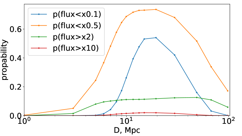
First, we examine the properties of the observed signal as a function of UHECR energy and a distance to the source. In Fig. 1 we show probability that at a given distance from the source UHECR flux differs from an average one in 2 or 10 times. One can see, that most probably the flux from the given source will be lower compared to the average one. For 10 % of sources it is at least two times higher while in up to 75% of cases it is 2 times smaller. Only in a few percent of cases (in knots) flux can be enhanced 10 times and more $F/F_{\mathrm{av}}>10$. On the other hand in up to 55 % of cases flux can be reduced in 10 times $F/F_{\mathrm{av}}<10$ in voids. This mean that for most of sources UHECR flux will stay same or will be reduced, while only for small fraction of sources it will be significantly increased, giving possibility to observe ’hot spot’ in the UHECR spectrum.

In Fig. 2 we show example of $E=10$ EeV proton fluxes relative to average one in the directions to knot, void and filament as function of the distance from the source. The black solid line marks an average flux $F=F_{\mathrm{av}}$. One can see that in example of Fig. 2 filament at knot have maximal flux at 12 Mpc from source and disappeared at 25-30 Mpc distance. Moreover, filament transforms to void between 30 Mpc and 50 Mpc from source.

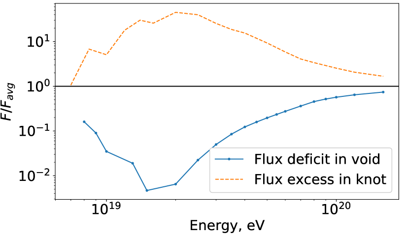
Finally we constructed the energy spectrum of the source for an observer located in the knot and in the filament, see Fig. 3. One can see that the observed flux deviates significantly from the average one at the energies around 10-30 EeV. These deviations disappear both at low and high energies. At the highest energies $\sim$ 100 EeV the deflections become too small to produce strong enough flux variations. On the other hand at low energy end of the spectrum UHECR propagation becomes diffusive which is also washing out the filamentary pattern.

III.2 Source images

The observer may have a sufficiently large radius compared to the distance to it, which introduces some distortions in the apparent size of the source when naively constructing a HealPy[22] map from the momentum of trapped particles. We remove this distortion by taking the projection of the particle’s momentum on the Oz axis of our basis, which is parallels to the direction to the source. The second vector of the basis is chosen manually. We complete the basis by taking the cross product of first and second vectors.

Figure 4: Source images seen by the observer located at knot and filament calculated at the edge of the Galaxy and after propagation through the GMF. Color encodes the number of hits to a given pixel. In both cases the intrinsic source luminosity is adjusted so that total number of events from the source observed at Earth matches with the cumulative number of TA events falling inside the hot spot circle of $25^{\circ}$ (44 events for the 15-year TA SD data). The blue color corresponds to the background level which is shown as uniform for clarity.

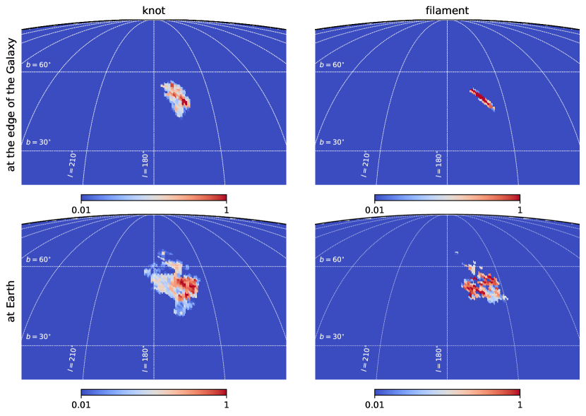
We have studied two cases of observer location 4: observer in a filament and observer in knot. We didn’t consider the most likely case of the void (it is about $\sim 70\%$, see Fig.1) as in this case the flux is extremely small and hard for detection. Knot case produces a bright smudged spot but this case is the most unlikely. Thus, if we have many sources of UHECR around us at a distance of tens Mpc, we see only a few of them. With respect to most sources, we will be in the voids. Sources at greater distances (more 100 Mpc) give an isotropic contribution, which decreases with distance and creates a uniform background.

On top right panel of Fig.4 you can see an image of the source when observer is located in a filament before propagation through the galactic magnetic field. in Ihis case the source has enough for detection flux and probability and an image which is very stretched. The elongation of the image is perpendicular to the spacial UHECR density filament and disappears when the energy is doubled. After passing the galactic magnetic field, a smeared spot could be formed as in bottom right panel Fig.4. The positions of the sources in the sky were chosen in a way to correspond to TA hotspot direction before GMF lensing. The final spots after GMF lensing have a size of about 20 degrees as known hotspots.

We performed analysis for 10-20 EeV protons here. Since UHECR at highest energies can be dominated by intermediate nuclei according to Auger data, propagation of protons at those energies would correspond to propagation of nuclei with Z times larger energies in the same magnetic fields, in particular UHECR with $E>57$ EeV would correspond to CNO nuclei.

As was shown for example in [23], CNO nuclei of required energies can reach us from up to 70 Mpc distance.

IV Conclusions

In this paper we studied influence of the intergalactic and Galactic magnetic fields on the images of nearby sources in the UHECR data. In particular we studied possibility to explain hot spots in UHECR data by contribution of nearby sources. In our previous paper [1] we have shown that the effects of UHECR propagation in a turbulent intergalactic magnetic field in the small-angle scattering regime produce non-trivial caustic-like pattern in the density of cosmic rays, with knots, filaments and voids in the density profile at given distance from source. Here we studied dependence of density profile from distance from source and from energy for fixed properties of magnetic field with strength 1 nG and coherence length 1 Mpc. We found that for large range of distances and energies of UHECR caustic-like pattern stays similar in the sky. This means that for given position of Milky Way galaxy in this pattern we have get (de-)amplification of original flux of source.

Final source images after propagation in the Galactic magnetic field are shown in Fig. 4. One can see that both knot and filament structures can provide final hot spots in the UHECR image, while location in the void significantly reduce contribution of given source in the observed UHECR flux.

For given class of UHECR sources we expect that most of nearby sources are located in the voids and we see only few of sources, which are located in the filaments. With small probability one can see even brighter amplification of sources flux in the knot.

Thus, in this work we show how hot spots in UHECR data can form. In Fig.4 we have shown examples of source image in the direction of TA hot spot. We show that after propagation in Galactic and inter-galactic magnetic fields source image can look like one observed in UHECR data. We performed analysis for 10 EeV protons, which would corresponds to CNO nuclei for energies of hot sport in TA and Auger data $E>57$ EeV. Source location at several tens of Mpc is still for CNO nuclei of those energies.

Acknowledgements.

Modeling of propagation of high-energy radiation in the Universe has been supported by the Russian Science Foundation grant 22-12-00253 (K.D. and G.R.). The work of K.D. has been supported by the fellowship of Basis Foundation (grant No. 22-1-5-92-1). The work of A.K. has been supported by the IISN project No. 4.4501.18. Some of the results in this paper have been derived using the healpy and HEALPix packages.

References

- Dolgikh et al. [2023] K. Dolgikh, A. Korochkin, G. Rubtsov, D. Semikoz, and I. Tkachev, J. Exp. Theor. Phys. 136, 704 (2023), arXiv:2212.01494 [astro-ph.HE] .
- Greisen [1966] K. Greisen, Phys. Rev. Lett. 16, 748 (1966).
- Zatsepin and Kuzmin [1966] G. T. Zatsepin and V. A. Kuzmin, JETP Lett. 4, 78 (1966), [Pisma Zh. Eksp. Teor. Fiz.4,114(1966)].
- Abbasi et al. [2008] R. U. Abbasi et al. (HiRes), Phys. Rev. Lett. 100, 101101 (2008), arXiv:astro-ph/0703099 .
- Abraham et al. [2008] J. Abraham et al. (Pierre Auger), Phys. Rev. Lett. 101, 061101 (2008), arXiv:0806.4302 [astro-ph] .
- Abu-Zayyad et al. [2013] T. Abu-Zayyad et al. (Telescope Array), Astrophys. J. Lett. 768, L1 (2013), arXiv:1205.5067 [astro-ph.HE] .
- Giacinti et al. [2010] G. Giacinti, M. Kachelriess, D. V. Semikoz, and G. Sigl, JCAP 08, 036 (2010), arXiv:1006.5416 [astro-ph.HE] .
- Giacinti et al. [2011] G. Giacinti, M. Kachelriess, D. V. Semikoz, and G. Sigl, Astropart. Phys. 35, 192 (2011), arXiv:1104.1141 [astro-ph.HE] .
- Yüksel et al. [2012] H. Yüksel, T. Stanev, M. D. Kistler, and P. P. Kronberg, Astrophys. J. 758, 16 (2012).
- Pshirkov et al. [2016] M. S. Pshirkov, P. G. Tinyakov, and F. R. Urban, Phys. Rev. Lett. 116, 191302 (2016), arXiv:1504.06546 [astro-ph.CO] .
- Katz et al. [2021] H. Katz et al., Mon. Not. Roy. Astron. Soc. 507, 1254 (2021), arXiv:2101.11624 [astro-ph.CO] .
- Jedamzik and Saveliev [2019] K. Jedamzik and A. Saveliev, Phys. Rev. Lett. 123, 021301 (2019), arXiv:1804.06115 [astro-ph.CO] .
- Note [1] https://github.com/okolo/mcray.
- Kalashev et al. [2023] O. Kalashev, A. Korochkin, A. Neronov, and D. Semikoz, Astron. Astrophys. 675, A132 (2023), arXiv:2201.03996 [astro-ph.HE] .
- Giacalone and Jokipii [1999] J. Giacalone and J. R. Jokipii, Astrophys. J. 520, 204 (1999).
- Jasche et al. [2020] J. Jasche, A. van Vliet, and J. P. Rachen, PoS ICRC2019, 447 (2020), arXiv:1911.05048 [astro-ph.HE] .
- Alves Batista et al. [2016] R. Alves Batista, A. Dundovic, M. Erdmann, K.-H. Kampert, D. Kuempel, G. Müller, G. Sigl, A. van Vliet, D. Walz, and T. Winchen, JCAP 05, 038 (2016), arXiv:1603.07142 [astro-ph.IM] .
- Alves Batista et al. [2022] R. Alves Batista et al., JCAP 09, 035 (2022), arXiv:2208.00107 [astro-ph.HE] .
- Jansson and Farrar [2012] R. Jansson and G. R. Farrar, Astrophys. J. 757, 14 (2012), arXiv:1204.3662 [astro-ph.GA] .
- Jansson and Farrar [2012] R. Jansson and G. R. Farrar, Astrophys. J. Lett. 761, L11 (2012), arXiv:1210.7820 [astro-ph.GA] .
- Note [2] Http://healpix.sf.net.
- Górski et al. [2005] K. M. Górski, E. Hivon, A. J. Banday, B. D. Wandelt, F. K. Hansen, M. Reinecke, and M. Bartelmann, Astrophys. J. 622, 759 (2005), arXiv:astro-ph/0409513 .
- Neronov et al. [2023] A. Neronov, D. Semikoz, and O. Kalashev, Phys. Rev. D 108, 103008 (2023), arXiv:2112.08202 [astro-ph.HE] .