UIEDP: Underwater Image Enhancement with Diffusion Prior

Abstract

Underwater image enhancement (UIE) aims to generate clear images from low-quality underwater images. Due to the unavailability of clear reference images, researchers often synthesize them to construct paired datasets for training deep models. However, these synthesized images may sometimes lack quality, adversely affecting training outcomes. To address this issue, we propose UIE with Diffusion Prior (UIEDP), a novel framework treating UIE as a posterior distribution sampling process of clear images conditioned on degraded underwater inputs. Specifically, UIEDP combines a pre-trained diffusion model capturing natural image priors with any existing UIE algorithm, leveraging the latter to guide conditional generation. The diffusion prior mitigates the drawbacks of inferior synthetic images, resulting in higher-quality image generation. Extensive experiments have demonstrated that our UIEDP yields significant improvements across various metrics, especially no-reference image quality assessment. And the generated enhanced images also exhibit a more natural appearance.

1 Introduction

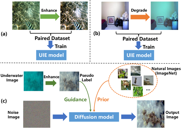
Figure 1: (a) Enhance real underwater images to obtain synthesized reference images, and construct paired samples for training UIE models. (b) Degrade natural images to obtain synthesized underwater images, and construct paired samples for training UIE models. (c) A diffusion model trained on ImageNet has natural image priors. To make full use of it, we guide the sampling process of the diffusion model with pseudo-labels generated by any UIE algorithm.

With the rise of marine ecological research and underwater archaeology, processing and understanding underwater images have attracted increasing attention. Due to the harsh underwater imaging conditions, underwater images usually suffer from various visual degradations, such as color casts, low contrast, and blurriness Ancuti et al. (2012); Ghani and Isa (2015). To enable advanced visual tasks like segmentation and detection of underwater images, underwater image enhancement (UIE) usually serves as a crucial preprocessing step Islam et al. (2020).

In recent years, deep learning-based methods have gradually outperformed traditional techniques in UIE. While many deep learning-based UIE models have been proposed Li et al. (2021); Guo et al. (2023); Jiang et al. (2023), they heavily rely on paired datasets for training. Due to the unavailability of clean reference images (also known as labels) for real underwater scenes, researchers have employed various approaches to synthesize paired datasets. One approach involves employing multiple UIE algorithms to enhance each underwater image and manually selecting the visually optimal result as the reference image Li et al. (2019a); Peng et al. (2023), as shown in Figure 1 (a). However, the upper limit of the reference image quality is limited by the chosen UIE algorithm. The alternative approach utilizes in-air images and corresponding depth maps to generate underwater-style images Wang et al. (2019); Li et al. (2020), as shown in Figure 1 (b). Nevertheless, the synthesized underwater-style images are unreal since the exact degradation model is unknown. To address these issues, some studies have explored domain adaptation to bridge the domain gap between synthetic and real images Chen and Pei (2022); Wang et al. (2023). However, such methods often introduce additional discriminators for adversarial training, potentially leading to training instability and mode collapse. Additionally, there are unsupervised Fu et al. (2022) and semi-supervised Huang et al. (2023) approaches that either forgo the use of paired datasets or rely on limited paired samples. However, their performance currently falls short of the state-of-the-art fully supervised methods.

Building upon the success of the diffusion model in various low-level visual tasks Kawar et al. (2022); Fei et al. (2023), we approach UIE as a conditional generation problem. Our objective is to model and sample the posterior probability density of the enhanced image given an underwater image. To achieve this, we propose UIEDP, a novel framework outlined in Figure 1 (c). Initially, we employ a diffusion model pre-trained on ImageNet Deng et al. (2009) as our generative model, which can capture the prior probability distribution of natural images. The denoising process of the diffusion model naturally generates realistic images. Subsequently, we utilize the output of any UIE algorithm as a pseudo-label image to guide the conditional generation, and sample from the posterior probability distribution of the enhanced image. If the UIE algorithm of generating pseudo labels is trained on synthetic paired datasets, the introduced diffusion prior can effectively counteract the adverse impact of unreal synthetic images. Furthermore, if the UIE algorithm does not require synthetic paired datasets training, the corresponding UIEDP is considered unsupervised. Experiments demonstrate that benefiting from the diffusion prior, the generated images consistently outperform both pseudo-label images and those produced by other UIE methods across various quality metrics.

In summary, our main contributions are twofold: (1) We design UIEDP, a novel diffusion-based framework for UIE from the perspective of conditional generation. UIEDP can make full use of the generative prior of the pre-trained diffusion model to generate higher-quality enhanced images. Notably, UIEDP is adaptable to both supervised and unsupervised settings, showcasing its versatility. (2) Extensive experiments and ablation studies demonstrate the effectiveness of our framework and illustrate the impact of each component.

2 Related Work

Underwater Image Enhancement.

Existing UIE methods can be divided into three categories: physical model-based, physical model-free, and data-driven methods. Physical model-based methods estimate the parameters of the underwater image formation model to invert the degradation process. For example, UDCP Drews et al. (2013) proposes a variant of DCP He et al. (2010) that estimates the transmission map through the blue and green color channels, while Galdran et al. Galdran et al. (2015) proposed a red channel method to recover colors associated to short wavelengths. Sea-thru Akkaynak and Treibitz (2019) replaces the atmospheric image formation model with a physically accurate model and restores color based on RGBD images. However, these methods are sensitive to the assumptions made in estimating the model parameters and thus have few applicable scenes and poor robustness. To improve the visual quality, physical model-free methods directly adjust image pixel values by histogram equalization Hitam et al. (2013), color balance Zhang et al. (2022); Ancuti et al. (2017), and contrast correlation Ghani and Isa (2015). Fusion Ancuti et al. (2012) is one typical method of these, which produces a more pleasing image by blending color-corrected and contrast-enhanced versions of the original underwater image. However, these methods often suffer from over-enhancement, color distortions, and artifacts when encountered with sophisticated illumination conditions Zhuang et al. (2022).

Recently, many works have focused on using deep learning techniques in UIE. However, obtaining reference images for underwater scenes is challenging, leading researchers to employ various methods to synthesize paired datasets. Li et al. Li et al. (2020) synthesized paired data based on underwater scene priors. Additionally, several GAN-based methods Fabbri et al. (2018); Islam et al. (2020) have been trained adversarially by the generated paired datasets. Li et al. Li et al. (2019a) constructed a paired dataset UIEB by using the best result of several enhancement algorithms to obtain a reference image. Peng et al. Peng et al. (2023) collected a larger dataset LSUI and used it to train a Transformer-based model. These paired datasets have facilitated the development of many UIE models. Some models have incorporated physical priors, such as multi-color space inputs Li et al. (2021); Wang et al. (2021) and depth maps Cong et al. (2023), to generate visually appealing images. To enhance the efficiency of UIE, Jiang et al. Jiang et al. (2023) proposed a highly efficient and lightweight real-time UIE network with only 9k parameters. In addition to these fully supervised methods, there are also unsupervised Fu et al. (2022) and semi-supervised Huang et al. (2023) methods.

Diffusion Models.

Denoising diffusion probabilistic model (DDPM) Ho et al. (2020) is a new generative framework that is utilized to model complex data distributions and generate high-quality images. Based on DDPM, the denoising diffusion implicit model (DDIM) Song et al. (2020) introduces a class of non-Markovian diffusion processes to accelerate the sampling process. In order to achieve conditional generation, Dhariwal et al. Dhariwal and Nichol (2021) have conditioned the pre-trained diffusion model during sampling with the gradients of a classifier. An alternative way is to explicitly introduce the conditional information as input to the diffusion models Saharia et al. (2022). Benefiting from conditional generation, the diffusion models have also been successfully applied to various image restoration tasks Fei et al. (2023), including denoising, deblurring, and inpainting Zhu et al. (2023); Lugmayr et al. (2022); Kawar et al. (2022). However, to our best knowledge, only Tang et al. Tang et al. (2023) have applied a lightweight diffusion model to underwater image enhancement in a supervised manner. In contrast, our approach does not train the diffusion model from scratch but rather makes full use of the natural image priors that are inherent in the pre-trained diffusion model. Furthermore, our method is also applicable to unsupervised scenarios.

3 Methodology

3.1 Preliminary of Diffusion Models

Denoising diffusion probabilistic model Sohl-Dickstein et al. (2015); Ho et al. (2020) is a type of generative model that converts the isotropic Gaussian distribution into a data distribution. It mainly consists of the diffusion process and the reverse process. The diffusion process is a Markov chain that gradually adds noise to data $x_{0}$ at $T$ time steps. Each step of the diffusion process can be written as:

$$q(x_{t}|x_{t-1})=\mathcal{N}(x_{t};\sqrt{1-\beta_{t}}x_{t-1},\beta_{t}\mathbf{I}),$$ (1)

where $\beta_{1},...,\beta_{T}$ is a fixed variance schedule. Using the notation $\alpha_{t}=1-\beta_{t}$ and $\overline{\alpha}_{t}=\prod_{s=1}^{t}\alpha_{s}$, we can sample $x_{t}$ at an arbitrary timestep according to a closed form:

$$x_{t}=\sqrt[]{\overline{\alpha}_{t}}x_{0}+\sqrt[]{1-\overline{\alpha}_{t}}\epsilon,$$ (2)

where $\epsilon$ is Gaussian noise.

To recover the data from the noise, each step of the reverse process can be defined as:

$$p_{\theta}(x_{t-1}|x_{t})=\mathcal{N}(x_{t-1};\mu_{\theta}(x_{t},t),{\Sigma}_{\theta}\mathbf{I}),$$ (3)

where $\mu_{\theta}(x_{t},t)$ is the mean, and variance ${\Sigma}_{\theta}$ can be set as learnable parameters Nichol and Dhariwal (2021) or constants Ho et al. (2020). By using reparameterization techniques, the mean can be transformed into:

$$\mu_{\theta}\left(x_{t},t\right)=\frac{1}{\sqrt{\alpha_{t}}}\left(x_{t}-\frac{\beta_{t}}{\sqrt{1-\bar{\alpha}_{t}}}\epsilon_{\theta}\left(x_{t},t\right)\right),$$ (4)

where $\epsilon_{\theta}$ is a function approximator intended to predict the noise $\epsilon$ in Equation 2 from $x_{t}$. By substituting the predicted noise $\epsilon_{\theta}\left(x_{t},t\right)$ into Equation 2, we can predict the data $\tilde{x}_{0}$ from $x_{t}$:

$$\tilde{x}_{0}=\frac{1}{\sqrt{\bar{\alpha}_{t}}}x_{t}-\frac{\sqrt{1-\bar{\alpha}_{t}}}{\sqrt{\bar{\alpha}_{t}}}\epsilon_{\theta}\left(x_{t},t\right).$$ (5)

To perform conditional generation, Dhariwal et al. Dhariwal and Nichol (2021) introduced a classifier $p_{\phi}(y|x_{t})$, and each step of the reverse process conditioned on $y$ can be rewritten as:

$$\begin{split}\log p_{\theta}\left(x_{t-1}|x_{t},y\right)&=\log\left(p_{\theta}\left(x_{t-1}|x_{t}\right)p_{\phi}\left(y|x_{t}\right)\right)+C_{1}\\ &\approx\log p(z)+C_{2},\end{split}$$ (6)

where $z\sim\mathcal{N}\left(\mu+\Sigma g,\Sigma\right)$, $\mu$ and $\Sigma$ are the mean and variance of the distribution $p_{\theta}\left(x_{t-1}|x_{t}\right)$ respectively. $C_{1}$ and $C_{2}$ are constants. $g$ is the gradient of the classifier:

$$g=\nabla_{x_{t}}\log p_{\phi}\left(y\mid x_{t}\right)|_{x_{t}=\mu}.$$ (7)

Therefore, the conditional transition operator can be approximated by shifting the mean at each time step by $\Sigma g$.

3.2 Proposed UIEDP

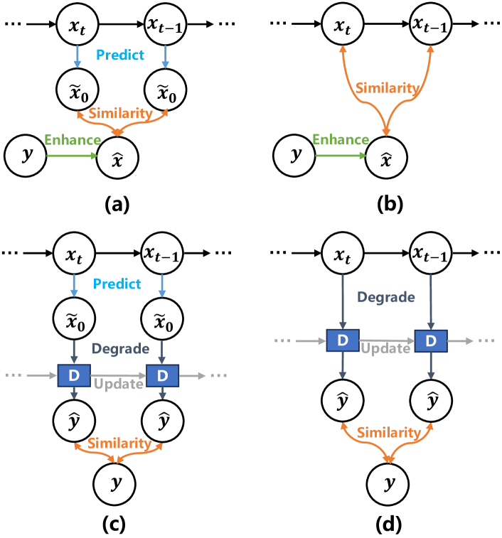
Figure 2: Four different guidance methods: guidance on (a) $\tilde{x}_{0}$ and natural image domain, (b) $x_{t}$ and natural image domain, (c) $\tilde{x}_{0}$ and underwater image domain, (d) $x_{t}$ and underwater image domain. The blue block D represents the underwater imaging model.

Given an underwater image $y$, the objective of UIE is to generate the enhanced image $x_{0}$ by searching within the domain of natural images $\mathcal{D}$ to discover a natural image $x_{0}$ that best matches $y$. Therefore, UIE can be conceptualized as sampling from the posterior probability, $p(x_{0}|y)$, conditioned on $y$. Due to the stronger generative capabilities demonstrated by diffusion models over other generative models, we utilize a DDPM pre-trained on ImageNet Deng et al. (2009) to establish the prior probability, $p(x_{0})$, within the natural image domain. Following Dhariwal et al. Dhariwal and Nichol (2021) and Equation 6, we can formulate each step in the reverse process (conditional sampling) as:

$$p_{\theta}\left(x_{t-1}|x_{t},y\right)=C_{3}p_{\theta}\left(x_{t-1}|x_{t}\right)p\left(y|x_{t}\right),$$ (8)

where $C_{3}$ is a constant. The former item $p_{\theta}\left(x_{t-1}|x_{t}\right)$ can be derived from the pre-trained diffusion model, capturing the transition probability from $x_{t}$ to $x_{t-1}$. $p_{\theta}\left(x_{t-1}|x_{t}\right)$ is a Gaussian distribution, and we use $\mu$ and $\Sigma$ to denote its mean and variance. Meanwhile, the latter item $p(y|x_{t})$ represents the guided item, which can be modeled by a classifier when $y$ corresponds to a specific category. However, in the context of UIE, the role of $p(y|x_{t})$ differs. Instead of categorization, we expect $p(y|x_{t})$ to quantify the degree of matching between the observed underwater image $y$ and the sampled image $x_{t}$. Following Avrahami et al. Avrahami et al. (2022), we directly model the negative logarithm of $p(y|x_{t})$ using a matching function $\mathcal{L}_{match}(y,x_{t})$:

$$-\log p(y|x_{t})=\mathcal{L}_{match}(y,x_{t}),$$ (9)

where the specific implementation of $\mathcal{L}_{match}(y,x_{t})$ is left to the following text. Substituting $\mathcal{L}_{match}(y,x_{t})$ into Equation 7, the new gradient of $p(y|x_{t})$ is:

$$g=-\nabla_{x}\mathcal{L}_{match}(y,x_{t})|_{x_{t}=\mu}.$$ (10)

Therefore, we can shift the mean $\mu$ by $\Sigma g$ during sampling to guide the generation. Next, we explore the design of the matching function $\mathcal{L}_{match}(y,x_{t})$, which determines the way guidance is applied.

Guidance on $\mathbf{x_{t}}$ or $\mathbf{\tilde{x}_{0}}$.

At each sampling step, in addition to the image $x_{t}$ sampled from the diffusion model, we also have $\tilde{x}_{0}$ which can be predicted from $x_{t}$. According to Equation 5, $\tilde{x}_{0}$ is known when $x_{t}$ is given. Therefore, $p(y|x_{t})=p(y|\tilde{x}_{0})$. Similarly, we can use the matching function $\mathcal{L}_{match}(y,\tilde{x}_{0})$ to model the negative logarithm of $p(y|\tilde{x}_{0})$, and the gradient $g$ can be calculated by $g=-\nabla_{\tilde{x}_{0}}\mathcal{L}_{match}(y,\tilde{x}_{0})$. Therefore, we have two different guidance methods: guidance on $x_{t}$ (Figure 2 (b) (d)) and guidance on $\tilde{x}_{0}$ (Figure 2 (a) (c)).

Whether the guidance is on $x_{t}$ ($x=x_{t}$) or $\tilde{x}_{0}$ ($x=\tilde{x}_{0}$), $x$ belongs to the natural image domain, whereas $y$ belongs to the underwater image domain. Hence, we need to transform $x$ and $y$ into the same domain before measuring the degree of matching $\mathcal{L}_{match}(y,x)$. Similar to Figure 1, there are two implementation approaches.

Guidance on Natural Image Domain.

We can transform $y$ into the natural image domain to align with $x$. As shown in Figure 2 (a) (b), we use any other UIE algorithm to enhance $y$ to generate the pseudo-label image $\hat{x}$. Then, we calculate the similarity $\mathcal{L}_{sim}(\hat{x},x)$ between the generated image and the pseudo-label image as the matching function $\mathcal{L}_{match}(y,x)$. It is worth noting that if the UIE algorithm used to generate the pseudo-label image $\hat{x}$ does not require supervised training, the corresponding UIEDP is also considered unsupervised.

Guidance on Underwater Image Domain.

We can also transform $x$ into the underwater image domain. Referring to the modified Koschmieder’s light scattering model Fu et al. (2022), the degradation of underwater images can be formulated as:

$$\hat{y}=x*T+(1-T)*A,$$ (11)

where $A$ is the global background light and $T$ is the medium transmission map representing the percentage of scene radiance reaching the camera after underwater reflection. For each underwater image, we estimate its $A$ by Gaussian blur Fu et al. (2022) and $T$ by GDCP Peng et al. (2018). However, the estimated transmission map may be inaccurate, resulting in an unrealistic underwater image $\hat{y}$. Inspired by Fei et al. Fei et al. (2023), we continually update $T$ by gradient descent at each sampling step. After obtaining $\hat{y}$, we calculate the similarity $\mathcal{L}_{sim}(y,\hat{y})$ between the real underwater image and the synthesized version as the matching function $\mathcal{L}_{match}(y,x)$, as shown in Figure 2 (c) (d). As no additional UIE algorithm is required, UIEDP which applies guidance on the underwater image domain is unsupervised.

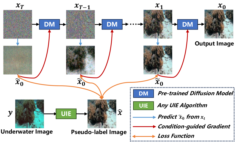
Figure 3: The overall framework of UIEDP. Guided by pseudo-labeled images generated from underwater imagery, a pre-trained diffusion model progressively denoises Gaussian noise images, yielding the corresponding enhanced images.

By selecting the variables ($x_{t}$ or $\tilde{x}_{0}$) and domains (natural or underwater) of the guidance, we have four different ways to implement the matching function $\mathcal{L}_{match}(y,x)$, as shown in Figure 2. We have conducted a comprehensive comparison and found that applying guidance on $\tilde{x}_{0}$ and natural image domain (Figure 2 (a)) is the best choice, as detailed in Section 4.4. Therefore, we implement UIEDP based on this guidance method.

Algorithm 1 UIEDP algorithm

0:  Underwater image $y$, any other UIE algorithm $\textup{Enhance}(\cdot)$, pre-trained diffusion model ($\mu_{\theta}(x_{t}),\Sigma_{\theta}(x_{t}),\epsilon_{\theta}(x_{t},t)$), loss function $\mathcal{L}$, and gradient scale $s$

0:  Enhanced image $x_{0}$

1:  $\hat{x}\leftarrow\textup{Enhance}(y)$

2:  Sample $x_{T}\sim\mathcal{N}(0,\mathbf{I})$

3:  for $t=T,...,1$ do

4:     $\mu,\Sigma\leftarrow\mu_{\theta}(x_{t}),\Sigma_{\theta}(x_{t})$

5:     $\tilde{x}_{0}\leftarrow\frac{1}{\sqrt{\bar{\alpha}_{t}}}x_{t}-\frac{\sqrt{1-\bar{\alpha}_{t}}}{\sqrt{\bar{\alpha}_{t}}}\epsilon_{\theta}\left(x_{t},t\right)$

6:     $g\leftarrow-\nabla_{\tilde{x}_{0}}\mathcal{L}(\hat{x},\tilde{x}_{0})$

7:     Sample $x_{t-1}\sim\mathcal{N}(\mu+sg,\Sigma)$

8:  end for

9:  return  $x_{0}$

As shown in Figure 3, we first utilize any other UIE algorithm to transform the underwater image $y$ into the natural image domain, getting the pseudo-label image $\hat{x}$. Then we predict the mean $\mu$ and $\tilde{x}_{0}$ from the sampled image $x_{t}$ at each sampling step. To improve the quality of the enhanced image, we add the image quality function of $\tilde{x}_{0}$ to the similarity function $\mathcal{L}_{sim}(\hat{x},\tilde{x}_{0})$ between $\hat{x}$ and $\tilde{x}_{0}$, obtaining the overall loss function $\mathcal{L}(\hat{x},\tilde{x}_{0})$. The gradient of the loss function $g=-\nabla_{\tilde{x}_{0}}\mathcal{L}(\hat{x},\tilde{x}_{0})$ is used to guide the conditional generation. Besides, we find that the variance $\Sigma$ negatively influences the generated image Fei et al. (2023). Therefore, we shift the mean $\mu$ by $sg$ instead of $s\Sigma g$, where $s$ is the gradient scale. Algorithm 1 summarizes the steps of our UIEDP algorithm, and algorithms about other three guidance methods (Figure 2 (b) (c) (d)) can be found in the appendix.

3.3 Loss Function

The loss function $\mathcal{L}(\hat{x},\tilde{x}_{0})$ is a key factor in guiding conditional generation, mainly composed of two parts: the similarity $\mathcal{L}_{sim}(\hat{x},\tilde{x}_{0})$ between $\hat{x}$ and $\tilde{x}_{0}$, and the quality of $\tilde{x}_{0}$.

Similarity between $\mathbf{\hat{x}}$ and $\mathbf{\tilde{x}_{0}}$.

In addition to the MAE loss $\mathcal{L}_{MAE}(\hat{x},\tilde{x}_{0})$, the similarity measure also incorporates the multiscale SSIM loss $\mathcal{L}_{MSSSIM}(\hat{x},\tilde{x}_{0})$ Wang et al. (2003) and the perceptual loss $\mathcal{L}_{Perceptual}(\hat{x},\tilde{x}_{0})$ Johnson et al. (2016). The multiscale SSIM loss mimics the human visual system to measure the multi-scale structural similarity of two images, while the perceptual loss measures the semantic content similarity at the feature level.

	T90					C60					U45
Methods	PSNR$\uparrow$	SSIM$\uparrow$	UCIQE$\uparrow$	UIQM$\uparrow$	NIQE$\downarrow$	URanker$\uparrow$	MUSIQ$\uparrow$	UCIQE$\uparrow$	UIQM$\uparrow$	NIQE$\downarrow$	URanker$\uparrow$	MUSIQ$\uparrow$	UCIQE$\uparrow$	UIQM$\uparrow$	NIQE$\downarrow$
GDCP	13.89	0.75	0.60	2.54	4.93	0.45	46.19	0.57	2.25	6.27	0.54	47.95	0.59	2.25	4.14
Fusion	23.14	0.89	0.63	2.86	4.98	1.43	44.74	0.61	2.61	5.91	1.68	47.62	0.64	2.97	8.02
UWCNN	19.02	0.82	0.55	2.79	4.72	0.56	42.13	0.51	2.52	5.94	0.36	46.96	0.48	3.04	4.09
UGAN	17.42	0.76	0.58	3.10	5.81	0.68	41.12	0.55	2.86	6.90	0.89	43.96	0.57	3.10	5.79
FUnIEGAN	16.97	0.73	0.57	3.06	4.92	0.42	41.55	0.55	2.87	6.06	0.80	45.68	0.56	2.92	4.45
MLLE	19.48	0.84	0.60	2.45	4.87	1.89	47.97	0.57	2.21	5.85	2.68	51.67	0.59	2.48	4.83
UShape	20.24	0.81	0.59	3.06	4.67	1.11	37.67	0.56	2.73	5.60	1.57	41.10	0.57	3.19	4.20
Ucolor	20.86	0.88	0.58	3.01	4.75	0.92	45.33	0.55	2.62	6.14	1.60	47.28	0.58	3.20	4.71
UIEC2Net	23.26	0.91	0.62	3.06	4.71	1.58	43.07	0.59	2.78	5.39	1.93	48.82	0.61	3.26	3.91
NU2Net	22.93	0.90	0.61	2.98	4.81	1.55	42.32	0.58	2.63	5.64	1.86	48.90	0.59	3.23	4.06
FA+Net	20.98	0.88	0.59	2.92	4.83	1.26	42.41	0.57	2.52	5.70	1.59	47.50	0.58	3.21	4.02
UIEDP	23.44	0.91	0.63	3.13	4.54	2.16	51.63	0.59	2.87	5.21	3.58	57.17	0.61	3.27	3.79

Table 1: Comparison with the state-of-the-art results on T90, C60, and U45. Bold and underlined denote the best and second-best results in each column, respectively. $\uparrow$ represents the higher is the better as well as $\downarrow$ represents the lower is the better.

Quality of $\mathbf{\tilde{x}_{0}}$.

URanker Guo et al. (2023) is a transformer trained on an underwater image quality ranking dataset, capable of producing quality scores for underwater images. MUSIQ Ke et al. (2021) is a popular Transformer-based natural image quality assessment (IQA) that has been proven to perform better than other traditional IQA metrics Huang et al. (2023). Therefore, we introduce these two differentiable losses: $\mathcal{L}_{URanker}(\tilde{x}_{0})$ and $\mathcal{L}_{MUSIQ}(\tilde{x}_{0})$.

The overall loss function $\mathcal{L}(\hat{x},\tilde{x}_{0})$ during sampling is a weighted sum of the above five losses:

$$\begin{split}\mathcal{L}(\hat{x},\tilde{x}_{0})&=\mathcal{L}_{MAE}(\hat{x},\tilde{x}_{0})-\lambda_{1}\mathcal{L}_{MSSSIM}(\hat{x},\tilde{x}_{0})\\ &+\lambda_{2}\mathcal{L}_{Perceptual}(\hat{x},\tilde{x}_{0})-\lambda_{3}\mathcal{L}_{URanker}(\tilde{x}_{0})\\ &-\lambda_{4}\mathcal{L}_{MUSIQ}(\tilde{x}_{0}),\end{split}$$ (12)

where $\lambda_{1}$, $\lambda_{2}$, $\lambda_{3}$ and $\lambda_{4}$ are hyper-parameters to balance the contribution of each loss.

4 Experiments

4.1 Datasets and Evaluation Metrics

We empirically evaluate the performance of UIEDP on two public datasets: UIEB Li et al. (2019a) and U45 Li et al. (2019b). The UIEB dataset consists of 890 raw underwater images and corresponding high-quality reference images. Following FA⁺Net Jiang et al. (2023), we use 800 pairs of these images as the training set, and the remaining 90 pairs of images as the test set, named T90. In addition, the UIEB dataset also includes a set of 60 challenge images (C60) that do not have corresponding reference images. The U45 dataset contains 45 carefully selected underwater images, serving as an important benchmark for UIE. For all the supervised methods, we train the models on the training set of UIEB and test them on the T90, C60, and U45 datasets.

In the above three test sets, each underwater image in T90 is paired with a corresponding reference image, while C60 and U45 only contain underwater images. Therefore, we evaluate the performance of UIE using two full-reference image quality evaluation metrics and five non-reference image quality assessment (NR-IQA) metrics. PSNR and SSIM are commonly used full-reference metrics for evaluating generation tasks, measuring the similarity between the enhanced images and the reference images. For non-reference metrics, we have adopted three metrics specifically designed for UIE tasks: UIQM Panetta et al. (2015), UCIQE Yang and Sowmya (2015), and URanker Guo et al. (2023), along with two natural image quality assessment metrics: NIQE Mittal et al. (2012) and MUSIQ Ke et al. (2021). UIQM considers contrast, sharpness, and colorfulness of the image, while UCIQE considers brightness instead of sharpness. NIQE analyzes the statistical properties of the image to measure the level of noise and distortion.

4.2 Implementation Details

We replicated all the compared methods based on their official codes and hyperparameters. For models requiring supervised training, we trained them for 100 epochs with a batch size of 32, using the ADAM optimizer Kingma and Ba (2014) with a learning rate 0.001. Data augmentation techniques such as horizontal flipping and rotation were employed during training. To ensure a fair comparison, all images were resized to 256$\times$256 during both training and testing. Our UIEDP loaded weights of the unconditional diffusion model pre-trained on the ImageNet dataset (at a resolution of 256$\times$256) provided by Dhariwal et al. Dhariwal and Nichol (2021). In all experiments, the weights $\lambda_{1}=1$, $\lambda_{2}=0.005$, $\lambda_{4}=0.00001$ in Equation 12. The gradient scale $s$ is set to 12000 on T90 and 4000 on the other two datasets. $\lambda_{3}$ is set to 0.002 on U45 and 0.001 on the other two datasets.

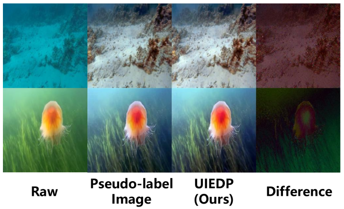
Figure 4: Comparison between the pseudo-labeled images and the images generated by UIEDP. The last column denotes their difference images.

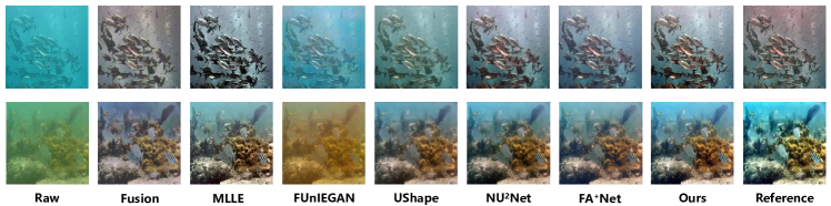
Figure 5: Visual comparison of different UIE methods on T90.

4.3 Comparison with the State-of-the-art

We compare our method UIEDP with several state-of-the-art approaches, including one physical model-based method (GDCP Peng et al. (2018)), two physical model-free methods (Fusion Ancuti et al. (2012), MLLE Zhang et al. (2022)), and eight data-driven methods (UWCNN Li et al. (2020), UGAN Fabbri et al. (2018), FUnIEGAN Islam et al. (2020), UShape Peng et al. (2023), UIEC²Net Wang et al. (2021), NU²Net Guo et al. (2023), FA⁺Net Jiang et al. (2023)). For our UIEDP, we employ UIEC²Net trained on the training set to generate pseudo-labeled images.

Results for three datasets are presented in Table 1. Experimental results demonstrate that compared to other methods, we achieve improvements in nearly all metrics across three datasets, particularly in NR-IQA metrics. It’s noteworthy that despite employing pseudo-labeled images generated by UIEC²Net for guiding conditional generation, UIEDP outperforms UIEC²Net across all metrics. This phenomenon can be attributed to UIEDP effectively harnessing the natural image priors inherent in the pre-trained diffusion model. Equation 8 indicates that conditional generation is jointly determined by priors and conditional guidance, thereby the introduction of diffusion prior enhances generation quality. Figure 4 visually illustrates the difference between output images of UIEDP and pseudo-labeled images. In the first example, the difference lies in the background lighting, with the image generated by UIEDP appearing brighter. In the second example, the difference lies in the jellyfish, where the image generated by UIEDP exhibits enhanced visual appeal.

Method	URanker$\uparrow$	MUSIQ$\uparrow$	UCIQE$\uparrow$	UIQM$\uparrow$	NIQE$\downarrow$
USUIR	1.20	42.85	0.57	2.65	5.89
Fusion	1.43	44.74	0.61	2.61	5.91
UIEDP (Fusion)	2.14	52.69	0.61	2.75	5.80

Table 2: Comparison with two unsupervised methods on C60.

Additionally, we present an intuitive comparison with other UIE methods in terms of visual effects. As shown in Figure 5, Fusion slightly distorts image colors and blurs image details; FUnIEGAN exhibits severe color distortion; MLLE renders images overly sharp, presenting a black-and-white tone; Ushape generates images with slightly dimmed background light; NU²Net and FA⁺Net fail to accommodate all underwater scenarios. For example, FA⁺Net performs well on the first example but poorly on the second. In contrast, the images generated by our UIEDP even appear better than the reference images, correcting the biased red or blue background light. This is attributed to the diffusion prior that is introduced by UIEDP. More visual comparisons are available in the appendix.

Fusion Ancuti et al. (2012) enhances underwater images by adjusting color and contrast without the need for supervised training. Therefore, if we employ Fusion to generate pseudo-labeled images in UIEDP, UIEDP (Fusion) is considered unsupervised. We compare UIEDP with Fusion and another deep learning-based unsupervised method, USUIR Fu et al. (2022), and the experimental results are presented in Table 2. We observe that even USUIR falls short compared to Fusion, indicating the considerable challenge of UIE in an unsupervised setting. Moreover, the performance of UIEDP surpasses both of the two other methods.

4.4 Ablation Study

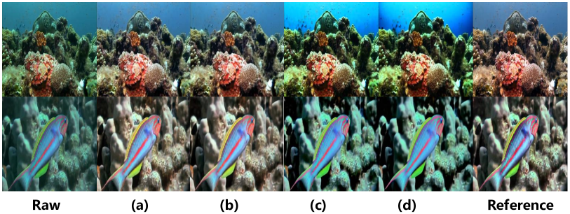
Figure 6: Visual comparison of four different guidance methods in Figure 2 on T90.

Guidance Method	PSNR$\uparrow$	SSIM$\uparrow$	UCIQE$\uparrow$	UIQM$\uparrow$	NIQE$\downarrow$	URanker$\uparrow$	MUSIQ$\uparrow$
Fig 2 (a) (Ours)	23.44	0.91	0.62	3.13	4.58	2.25	47.63
Fig 2 (b)	23.06	0.89	0.62	3.10	4.94	2.29	46.33
Fig 2 (c)	17.50	0.76	0.63	2.55	4.79	1.76	45.58
Fig 2 (d)	16.93	0.73	0.63	2.51	5.53	1.83	43.18

Table 3: Comparison of different guidance methods in Fig 2 on T90.

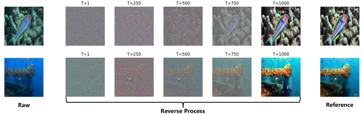
Figure 7: Visualization of the inverse diffusion process of UIEDP. The output images at 1000 steps are the final enhanced images.

Ablations about guidance methods.

In Figure 2, we propose four different guidance methods. Guidance can act on various variables ($x_{t}$ or $\tilde{x}_{0}$) and image domains (natural or underwater). To find the optimal guidance method, we conduct both quantitative and qualitative analyses. For fair comparison, we omit quality assessment losses $\mathcal{L}_{MUSIQ}$ and $\mathcal{L}_{URanker}$ in this ablation experiment. As shown in the last two rows of Table 3 and in Figure 6 (c) (d), guidance in the underwater image domain fails. This is because the degradation model in Equation 11 is a simplified imaging model that cannot precisely model real underwater imaging. And estimated global illumination and transmission maps may also be inaccurate. From Figure 6 (c) (d), the background light of the enhanced images is not normal. Although Figure 6 (a) and (b) looks visually similar, results in the first two rows of Table 3 suggest that guidance on $\tilde{x}_{0}$ yields better results than guidance on $x_{t}$. This is because in the early sampling steps, while $x_{t}$ still appears as a noisy image, $\tilde{x}_{0}$ already resembles the outline of a normal image, as illustrated in Figure 3. From the above analysis, we find that applying guidance on $\tilde{x}_{0}$ and natural image domain (Figure 2 (a)) is the optimal guidance method.

Impact of the loss function.

The loss function $\mathcal{L}(\hat{x},\tilde{x}_{0})$ plays a critical role in the sampling process, guiding conditional generation through its gradients. In UIEDP, we utilize a weighted sum of five losses as the total loss function $\mathcal{L}(\hat{x},\tilde{x}_{0})$. To investigate their contributions, we progressively introduce four additional losses alongside the MAE loss $\mathcal{L}_{MAE}$ for experimental analysis. The comprehensive experimental results are detailed in Table 4. Notably, the inclusion of multiscale SSIM loss $\mathcal{L}_{MSSSIM}$ and perceptual loss $\mathcal{L}_{Perceptual}$ both positively impact the generation process. These losses holistically gauge the similarity between generated images $\tilde{x}_{0}$ and pseudo-labeled images $\hat{x}$ from various perspectives, leading to enhanced generation quality. Furthermore, MUSIQ $\mathcal{L}_{MUSIQ}$ and URanker $\mathcal{L}_{URanker}$ losses significantly elevate the non-reference quality assessment for the generated images. Additionally, despite conditional generation being guided by pseudo-labeled images, UIEDP can produce higher-quality images compared to the provided pseudo-labeled images. This highlights that the pre-trained diffusion model on ImageNet inherently yields high-quality image outputs, which helps enhance low-quality underwater images.

Loss Function	PSNR$\uparrow$	SSIM$\uparrow$	UCIQE$\uparrow$	UIQM$\uparrow$	NIQE$\downarrow$	URanker$\uparrow$	MUSIQ$\uparrow$
Pseudo-label	23.26	0.91	0.62	3.06	4.71	2.20	47.71
$\mathcal{L}_{MAE}$	23.40	0.91	0.62	3.10	4.77	2.27	47.56
+$\mathcal{L}_{MSSSIM}$	23.42	0.91	0.62	3.10	4.72	2.27	47.55
+$\mathcal{L}_{Perceptual}$	23.44	0.91	0.62	3.13	4.58	2.25	47.63
+$\mathcal{L}_{URanker}$	23.43	0.91	0.62	3.12	4.60	2.44	47.77
+$\mathcal{L}_{MUSIQ}$	23.44	0.91	0.63	3.13	4.54	2.43	50.98

Table 4: Impact of the loss function $\mathcal{L}(\hat{x},\tilde{x}_{0})$ on T90. The first row indicates the quality of pseudo-labeled images, and the other rows indicate the quality of enhanced images generated by UIEDP under the guidance of different loss functions.

Method	Total steps	PSNR$\uparrow$	SSIM$\uparrow$	UCIQE$\uparrow$	UIQM$\uparrow$	NIQE$\downarrow$
DDIM	25	21.63	0.85	0.63	2.93	5.65
	50	20.08	0.79	0.64	2.94	5.66
DDPM	50	18.50	0.66	0.61	3.06	4.95
	250	22.40	0.88	0.62	3.12	4.69
	1000 (Ours)	23.44	0.91	0.63	3.13	4.54

Table 5: Effect of sampling strategies and steps on T90.

Effect of sampling strategies and steps.

DDIM Song et al. (2020) improves the sampling process over DDPM, allowing the generation of images of comparable quality with fewer steps. To explore the effect of sampling strategies, we replace the sampling process of UIEDP with DDIM. Experimental results in Table 5 indicate that images sampled via DDIM demonstrate inferior quality compared to DDPM. Additionally, in an effort to expedite generation speed, we attempt to directly reduce sampling steps. For DDIM, appropriately reducing the sampling steps yields better results. However, reducing the sampling steps for DDPM leads to a decrease in the quality of generated images. In Figure 7, we visualize the images sampled from the intermediate steps when the total number of steps is 1000. Exploring how to enhance sampling efficiency is left for future research.

5 Conclusion

We propose a novel framework UIEDP for underwater image enhancement, which combines the pre-train diffusion model and any UIE algorithm to conduct conditional generation. The pre-trained diffusion model introduces the natural image prior, ensuring the capability to generate high-quality images. Simultaneously, any UIE algorithm provides pseudo-label images to guide conditional sampling, facilitating the generation of enhanced versions corresponding to underwater images. Additionally, UIEDP can work in either a supervised or unsupervised manner, depending on whether the UIE algorithm generating pseudo-labeled images requires paired samples for training. Extensive experiments show that UIEDP not only generates enhanced images of superior quality beyond the pseudo-labeled images but also surpasses other advanced UIE methods.

Appendix A Limitations and Future Work

Like other diffusion-based methods, the primary drawback of UIEDP is the requirement for many sampling steps, hindering its application in scenarios that demand real-time enhancement. Hence, future research will focus on enhancing the generation efficiency of UIEDP. In the realm of diffusion models, several works have tried to generate high-quality images with fewer sampling steps. Exploring the application of acceleration techniques employed in these studies to enhance the efficiency of UIEDP stands as a promising avenue for exploration.

Appendix B More Algorithms

In this section, we elaborate on the implementation of three other guidance methods mentioned in Figure 2 of the main paper, along with the integration of DDIM within UIEDP. Algorithms 2, 3, 4 correspond to the three guidance methods depicted in Figure 2 (b) (c) (d), respectively. Algorithm 5 delineates the steps involved in utilizing DDIM for sampling within UIEDP.

Algorithm 2 Guidance on $x_{t}$ and natural image domain

0:  Underwater image $y$, any other UIE algorithm $\textup{Enhance}(\cdot)$, pre-trained diffusion model ($\mu_{\theta}(x_{t}),\Sigma_{\theta}(x_{t})$), loss function $\mathcal{L}$, and gradient scale $s$

0:  Enhanced image $x_{0}$

1:  $\hat{x}\leftarrow\textup{Enhance}(y)$

2:  Sample $x_{T}\sim\mathcal{N}(0,\mathbf{I})$

3:  for $t=T,...,1$ do

4:     $\mu,\Sigma\leftarrow\mu_{\theta}(x_{t}),\Sigma_{\theta}(x_{t})$

5:     $g\leftarrow-\nabla_{x_{t}}\mathcal{L}(\hat{x},x_{t})$

6:     Sample $x_{t-1}\sim\mathcal{N}(\mu+sg,\Sigma)$

7:  end for

8:  return  $x_{0}$

Algorithm 3 Guidance on $\tilde{x}_{0}$ and underwater image domain

0:  Underwater image $y$, global background light $A$, transmission map $T$, learning rate $l$ for optimizing $T$, pre-trained diffusion model ($\mu_{\theta}(x_{t}),\Sigma_{\theta}(x_{t}),\epsilon_{\theta}(x_{t},t)$), loss function $\mathcal{L}$, and gradient scale $s$

0:  Enhanced image $x_{0}$

1:  Sample $x_{T}\sim\mathcal{N}(0,\mathbf{I})$

2:  for $t=T,...,1$ do

3:     $\mu,\Sigma\leftarrow\mu_{\theta}(x_{t}),\Sigma_{\theta}(x_{t})$

4:     $\tilde{x}_{0}\leftarrow\frac{1}{\sqrt{\bar{\alpha}_{t}}}x_{t}-\frac{\sqrt{1-\bar{\alpha}_{t}}}{\sqrt{\bar{\alpha}_{t}}}\epsilon_{\theta}\left(x_{t},t\right)$

5:     $\hat{y}\leftarrow\tilde{x}_{0}*T+(1-T)*A$

6:     $T\leftarrow T-l\nabla_{T}\mathcal{L}(y,\hat{y})$

7:     $g\leftarrow-\nabla_{\tilde{x}_{0}}\mathcal{L}(y,\hat{y})$

8:     Sample $x_{t-1}\sim\mathcal{N}(\mu+sg,\Sigma)$

9:  end for

10:  return  $x_{0}$

Algorithm 4 Guidance on $x_{t}$ and underwater image domain

0:  Underwater image $y$, global background light $A$, transmission map $T$, learning rate $l$ for optimizing $T$, pre-trained diffusion model ($\mu_{\theta}(x_{t}),\Sigma_{\theta}(x_{t})$), loss function $\mathcal{L}$, and gradient scale $s$

0:  Enhanced image $x_{0}$

1:  $\hat{x}\leftarrow\textup{Enhance}(y)$

2:  Sample $x_{T}\sim\mathcal{N}(0,\mathbf{I})$

3:  for $t=T,...,1$ do

4:     $\mu,\Sigma\leftarrow\mu_{\theta}(x_{t}),\Sigma_{\theta}(x_{t})$

5:     $\hat{y}\leftarrow x_{t}*T+(1-T)*A$

6:     $T\leftarrow T-l\nabla_{T}\mathcal{L}(y,\hat{y})$

7:     $g\leftarrow-\nabla_{x_{t}}\mathcal{L}(y,\hat{y})$

8:     Sample $x_{t-1}\sim\mathcal{N}(\mu+sg,\Sigma)$

9:  end for

10:  return  $x_{0}$

Algorithm 5 UIEDP algorithm with DDIM sampling strategy

0:  Underwater image $y$, any other UIE algorithm $\textup{Enhance}(\cdot)$, pre-trained diffusion model $\epsilon_{\theta}(x_{t},t)$, loss function $\mathcal{L}$, and gradient scale $s$

0:  Enhanced image $x_{0}$

1:  $\hat{x}\leftarrow\textup{Enhance}(y)$

2:  Sample $x_{T}\sim\mathcal{N}(0,\mathbf{I})$

3:  for $t=T,...,1$ do

4:     $\tilde{x}_{0}\leftarrow\frac{1}{\sqrt{\bar{\alpha}_{t}}}x_{t}-\frac{\sqrt{1-\bar{\alpha}_{t}}}{\sqrt{\bar{\alpha}_{t}}}\epsilon_{\theta}\left(x_{t},t\right)$

5:     $g\leftarrow-\nabla_{\tilde{x}_{0}}\mathcal{L}(\hat{x},\tilde{x}_{0})$

6:     $\hat{\epsilon}\leftarrow\epsilon_{\theta}(x_{t},t)-\sqrt{1-\bar{\alpha}_{t}}sg$

7:     $x_{t-1}\leftarrow\sqrt{\bar{\alpha}_{t-1}}(\frac{x_{t}-\sqrt{1-\bar{\alpha}_{t}}\hat{\epsilon}}{\sqrt{\bar{\alpha}_{t}}})+\sqrt{1-\bar{\alpha}_{t-1}}\hat{\epsilon}$

8:  end for

9:  return  $x_{0}$

Appendix C More ablations

In this section, we conducted more ablations to further validate the effectiveness of UIEDP.

Ablations about other UIE algorithms.

In the main paper, we utilize UIEC²Net and Fusion as the algorithms responsible for generating pseudo-labeled images in UIEDP. We observe consistent improvements in image quality generated by UIEDP compared to the pseudo-labeled images. Consequently, we replace the algorithms generating pseudo-labeled images with MLLE and FA⁺Net to ascertain if this improvement persisted. The experimental results are presented in Table 6. Our findings indicate that irrespective of the UIE algorithm integrated into UIEDP, it consistently generates superior enhanced images, which further emphasizes the effectiveness of the diffusion prior.

Ablations about the variance $\Sigma$.

During the conditional sampling process, we omitted one coefficient of gradient, i.e., the distribution variance $\Sigma$ predicted by the diffusion model. According to the experimental results in Table 7, we find that the variance $\Sigma$ negatively influences the generated images. Hence, we shift the mean by $sg$ instead of $s\Sigma g$.

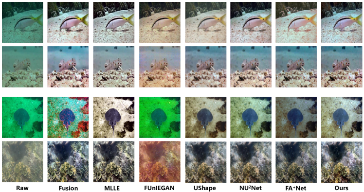
Figure 8: Visual comparison of different UIE methods on C60 and U45.

	PSNR$\uparrow$	SSIM$\uparrow$	UCIQE$\uparrow$	UIQM$\uparrow$	NIQE$\downarrow$
MLLE	19.48	0.84	0.60	2.45	4.87
UIEDP (MLLE)	19.91	0.85	0.60	2.53	4.65
FA+Net	20.98	0.88	0.59	2.92	4.83
UIEDP (FA+Net)	21.05	0.88	0.60	3.05	4.64

Table 6: Ablations about other UIE algorithms on T90.

	PSNR$\uparrow$	SSIM$\uparrow$	UCIQE$\uparrow$	UIQM$\uparrow$	NIQE$\downarrow$
with $\Sigma$	22.98	0.90	0.62	3.03	4.60
without $\Sigma$	23.44	0.91	0.63	3.13	4.54

Table 7: Ablations about the variance $\Sigma$ on T90.

Appendix D More Visual Results

As shown in Figure 8, we present an intuitive comparison with other UIE methods in terms of visual effects. The first two rows are samples from C60, and the last two rows are samples from U45.

References

- Akkaynak and Treibitz [2019] Derya Akkaynak and Tali Treibitz. Sea-thru: A method for removing water from underwater images. In Proceedings of the IEEE/CVF conference on computer vision and pattern recognition, pages 1682–1691, 2019.
- Ancuti et al. [2012] Cosmin Ancuti, Codruta Orniana Ancuti, Tom Haber, and Philippe Bekaert. Enhancing underwater images and videos by fusion. In 2012 IEEE conference on computer vision and pattern recognition, pages 81–88. IEEE, 2012.
- Ancuti et al. [2017] Codruta O Ancuti, Cosmin Ancuti, Christophe De Vleeschouwer, and Philippe Bekaert. Color balance and fusion for underwater image enhancement. IEEE Transactions on image processing, 27(1):379–393, 2017.
- Avrahami et al. [2022] Omri Avrahami, Dani Lischinski, and Ohad Fried. Blended diffusion for text-driven editing of natural images. In Proceedings of the IEEE/CVF Conference on Computer Vision and Pattern Recognition (CVPR), pages 18208–18218, June 2022.
- Chen and Pei [2022] Yu-Wei Chen and Soo-Chang Pei. Domain adaptation for underwater image enhancement via content and style separation. IEEE Access, 10:90523–90534, 2022.
- Cong et al. [2023] Runmin Cong, Wenyu Yang, Wei Zhang, Chongyi Li, Chun-Le Guo, Qingming Huang, and Sam Kwong. Pugan: Physical model-guided underwater image enhancement using gan with dual-discriminators. IEEE Transactions on Image Processing, 2023.
- Deng et al. [2009] Jia Deng, Wei Dong, Richard Socher, Li-Jia Li, Kai Li, and Li Fei-Fei. Imagenet: A large-scale hierarchical image database. In 2009 IEEE conference on computer vision and pattern recognition, pages 248–255. Ieee, 2009.
- Dhariwal and Nichol [2021] Prafulla Dhariwal and Alexander Nichol. Diffusion models beat gans on image synthesis. Advances in neural information processing systems, 34:8780–8794, 2021.
- Drews et al. [2013] Paul Drews, Erickson Nascimento, Filipe Moraes, Silvia Botelho, and Mario Campos. Transmission estimation in underwater single images. In Proceedings of the IEEE international conference on computer vision workshops, pages 825–830, 2013.
- Fabbri et al. [2018] Cameron Fabbri, Md Jahidul Islam, and Junaed Sattar. Enhancing underwater imagery using generative adversarial networks. In 2018 IEEE international conference on robotics and automation (ICRA), pages 7159–7165. IEEE, 2018.
- Fei et al. [2023] Ben Fei, Zhaoyang Lyu, Liang Pan, Junzhe Zhang, Weidong Yang, Tianyue Luo, Bo Zhang, and Bo Dai. Generative diffusion prior for unified image restoration and enhancement. In Proceedings of the IEEE/CVF Conference on Computer Vision and Pattern Recognition, pages 9935–9946, 2023.
- Fu et al. [2022] Zhenqi Fu, Huangxing Lin, Yan Yang, Shu Chai, Liyan Sun, Yue Huang, and Xinghao Ding. Unsupervised underwater image restoration: From a homology perspective. In Proceedings of the AAAI Conference on Artificial Intelligence, volume 36, pages 643–651, 2022.
- Galdran et al. [2015] Adrian Galdran, David Pardo, Artzai Picón, and Aitor Alvarez-Gila. Automatic red-channel underwater image restoration. Journal of Visual Communication and Image Representation, 26:132–145, 2015.
- Ghani and Isa [2015] Ahmad Shahrizan Abdul Ghani and Nor Ashidi Mat Isa. Enhancement of low quality underwater image through integrated global and local contrast correction. Applied Soft Computing, 37:332–344, 2015.
- Guo et al. [2023] Chunle Guo, Ruiqi Wu, Xin Jin, Linghao Han, Weidong Zhang, Zhi Chai, and Chongyi Li. Underwater ranker: Learn which is better and how to be better. In Proceedings of the AAAI conference on artificial intelligence, volume 37, pages 702–709, 2023.
- He et al. [2010] Kaiming He, Jian Sun, and Xiaoou Tang. Single image haze removal using dark channel prior. IEEE transactions on pattern analysis and machine intelligence, 33(12):2341–2353, 2010.
- Hitam et al. [2013] Muhammad Suzuri Hitam, Ezmahamrul Afreen Awalludin, Wan Nural Jawahir Hj Wan Yussof, and Zainuddin Bachok. Mixture contrast limited adaptive histogram equalization for underwater image enhancement. In 2013 International conference on computer applications technology (ICCAT), pages 1–5. IEEE, 2013.
- Ho et al. [2020] Jonathan Ho, Ajay Jain, and Pieter Abbeel. Denoising diffusion probabilistic models. Advances in neural information processing systems, 33:6840–6851, 2020.
- Huang et al. [2023] Shirui Huang, Keyan Wang, Huan Liu, Jun Chen, and Yunsong Li. Contrastive semi-supervised learning for underwater image restoration via reliable bank. In Proceedings of the IEEE/CVF Conference on Computer Vision and Pattern Recognition, pages 18145–18155, 2023.
- Islam et al. [2020] Md Jahidul Islam, Youya Xia, and Junaed Sattar. Fast underwater image enhancement for improved visual perception. IEEE Robotics and Automation Letters, 5(2):3227–3234, 2020.
- Jiang et al. [2023] Jingxia Jiang, Tian Ye, Jinbin Bai, Sixiang Chen, Wenhao Chai, Shi Jun, Yun Liu, and Erkang Chen. Five a+ network: You only need 9k parameters for underwater image enhancement. arXiv preprint arXiv:2305.08824, 2023.
- Johnson et al. [2016] Justin Johnson, Alexandre Alahi, and Li Fei-Fei. Perceptual losses for real-time style transfer and super-resolution. In Computer Vision–ECCV 2016: 14th European Conference, Amsterdam, The Netherlands, October 11-14, 2016, Proceedings, Part II 14, pages 694–711. Springer, 2016.
- Kawar et al. [2022] Bahjat Kawar, Michael Elad, Stefano Ermon, and Jiaming Song. Denoising diffusion restoration models. Advances in Neural Information Processing Systems, 35:23593–23606, 2022.
- Ke et al. [2021] Junjie Ke, Qifei Wang, Yilin Wang, Peyman Milanfar, and Feng Yang. Musiq: Multi-scale image quality transformer. In Proceedings of the IEEE/CVF International Conference on Computer Vision, pages 5148–5157, 2021.
- Kingma and Ba [2014] Diederik P Kingma and Jimmy Ba. Adam: A method for stochastic optimization. In International Conference on Learning Representations, 2014.
- Li et al. [2019a] Chongyi Li, Chunle Guo, Wenqi Ren, Runmin Cong, Junhui Hou, Sam Kwong, and Dacheng Tao. An underwater image enhancement benchmark dataset and beyond. IEEE Transactions on Image Processing, 29:4376–4389, 2019.
- Li et al. [2019b] Hanyu Li, Jingjing Li, and Wei Wang. A fusion adversarial underwater image enhancement network with a public test dataset. arXiv preprint arXiv:1906.06819, 2019.
- Li et al. [2020] Chongyi Li, Saeed Anwar, and Fatih Porikli. Underwater scene prior inspired deep underwater image and video enhancement. Pattern Recognition, 98:107038, 2020.
- Li et al. [2021] Chongyi Li, Saeed Anwar, Junhui Hou, Runmin Cong, Chunle Guo, and Wenqi Ren. Underwater image enhancement via medium transmission-guided multi-color space embedding. IEEE Transactions on Image Processing, 30:4985–5000, 2021.
- Lugmayr et al. [2022] Andreas Lugmayr, Martin Danelljan, Andres Romero, Fisher Yu, Radu Timofte, and Luc Van Gool. Repaint: Inpainting using denoising diffusion probabilistic models. In Proceedings of the IEEE/CVF Conference on Computer Vision and Pattern Recognition, pages 11461–11471, 2022.
- Mittal et al. [2012] Anish Mittal, Rajiv Soundararajan, and Alan C Bovik. Making a “completely blind” image quality analyzer. IEEE Signal processing letters, 20(3):209–212, 2012.
- Nichol and Dhariwal [2021] Alexander Quinn Nichol and Prafulla Dhariwal. Improved denoising diffusion probabilistic models. In International Conference on Machine Learning, pages 8162–8171. PMLR, 2021.
- Panetta et al. [2015] Karen Panetta, Chen Gao, and Sos Agaian. Human-visual-system-inspired underwater image quality measures. IEEE Journal of Oceanic Engineering, 41(3):541–551, 2015.
- Peng et al. [2018] Yan-Tsung Peng, Keming Cao, and Pamela C Cosman. Generalization of the dark channel prior for single image restoration. IEEE Transactions on Image Processing, 27(6):2856–2868, 2018.
- Peng et al. [2023] Lintao Peng, Chunli Zhu, and Liheng Bian. U-shape transformer for underwater image enhancement. IEEE Transactions on Image Processing, 2023.
- Saharia et al. [2022] Chitwan Saharia, Jonathan Ho, William Chan, Tim Salimans, David J Fleet, and Mohammad Norouzi. Image super-resolution via iterative refinement. IEEE Transactions on Pattern Analysis and Machine Intelligence, 45(4):4713–4726, 2022.
- Sohl-Dickstein et al. [2015] Jascha Sohl-Dickstein, Eric Weiss, Niru Maheswaranathan, and Surya Ganguli. Deep unsupervised learning using nonequilibrium thermodynamics. In International conference on machine learning, pages 2256–2265. PMLR, 2015.
- Song et al. [2020] Jiaming Song, Chenlin Meng, and Stefano Ermon. Denoising diffusion implicit models. arXiv preprint arXiv:2010.02502, 2020.
- Tang et al. [2023] Yi Tang, Hiroshi Kawasaki, and Takafumi Iwaguchi. Underwater image enhancement by transformer-based diffusion model with non-uniform sampling for skip strategy. In Proceedings of the 31st ACM International Conference on Multimedia, pages 5419–5427, 2023.
- Wang et al. [2003] Zhou Wang, Eero P Simoncelli, and Alan C Bovik. Multiscale structural similarity for image quality assessment. In The Thrity-Seventh Asilomar Conference on Signals, Systems & Computers, 2003, volume 2, pages 1398–1402. Ieee, 2003.
- Wang et al. [2019] Nan Wang, Yabin Zhou, Fenglei Han, Haitao Zhu, and Jingzheng Yao. Uwgan: underwater gan for real-world underwater color restoration and dehazing. arXiv preprint arXiv:1912.10269, 2019.
- Wang et al. [2021] Yudong Wang, Jichang Guo, Huan Gao, and Huihui Yue. Uiec2-net: Cnn-based underwater image enhancement using two color space. Signal Processing: Image Communication, 96:116250, 2021.
- Wang et al. [2023] Zhengyong Wang, Liquan Shen, Mai Xu, Mei Yu, Kun Wang, and Yufei Lin. Domain adaptation for underwater image enhancement. IEEE Transactions on Image Processing, 32:1442–1457, 2023.
- Yang and Sowmya [2015] Miao Yang and Arcot Sowmya. An underwater color image quality evaluation metric. IEEE Transactions on Image Processing, 24(12):6062–6071, 2015.
- Zhang et al. [2022] Weidong Zhang, Peixian Zhuang, Hai-Han Sun, Guohou Li, Sam Kwong, and Chongyi Li. Underwater image enhancement via minimal color loss and locally adaptive contrast enhancement. IEEE Transactions on Image Processing, 31:3997–4010, 2022.
- Zhu et al. [2023] Yuanzhi Zhu, Kai Zhang, Jingyun Liang, Jiezhang Cao, Bihan Wen, Radu Timofte, and Luc Van Gool. Denoising diffusion models for plug-and-play image restoration. In Proceedings of the IEEE/CVF Conference on Computer Vision and Pattern Recognition, pages 1219–1229, 2023.
- Zhuang et al. [2022] Peixian Zhuang, Jiamin Wu, Fatih Murat Porikli, and Chongyi Li. Underwater image enhancement with hyper-laplacian reflectance priors. IEEE Transactions on Image Processing, 31:5442–5455, 2022.