CSST Strong Lensing Preparation: Forecast the galaxy-galaxy strong lensing population for the China Space Station Telescope

Abstract

Galaxy-galaxy strong gravitational lens (GGSL) is a powerful probe for the formation and evolution of galaxies and cosmology, while the sample size of GGSLs leads to considerable uncertainties and potential bias. The China Space Station Telescope (CSST, planned to be launched in 2025) will conduct observations across 17,500 square degrees of the sky, capturing images in the $ugriz$ bands with a spatial resolution comparable to that of the Hubble Space Telescope (HST). We ran a set of Monte Carlo simulations to predict that the CSST’s wide-field survey will observe $\sim$160,000 galaxy-galaxy strong lenses over the lifespan, expanding the number of existing galaxy-galaxy lens samples by three orders of magnitude, which is comparable to the Euclid telescope launched during the same period but with additional color information. Specifically, the CSST can detect strong lenses with Einstein radii above $0.64\pm 0.42\arcsec$, corresponding to the velocity dispersions of $217.19\pm 50.55\,\text{km/s}$. These lenses exhibit a median magnification of $\sim$5. The apparent magnitude of the unlensed source in the g-band is $25.87\pm 1.19$. The signal-to-noise ratio of the lensed images covers a range of $\sim 20$ to $\sim 1000$, allowing us to determine the Einstein radius with an accuracy ranging from $\sim 1\%$ to $\sim 0.1\%$, ignoring various modeling systematics. Besides, our estimations show that CSST can observe uncommon systems, such as double source-plane and spiral galaxy lenses. The above selection functions of the CSST strong lensing observation help optimize the strategy of finding and modeling GGSLs.

1 Introduction

Galaxy-galaxy strong gravitational lensing is a phenomenon in which the gravitational field of a foreground lens galaxy significantly distorts the light emitted from a background source galaxy, leading to the formation of multiple images or extended arc structures. Lens modeling enables the reconstruction of both the mass distribution of the lens and the intrinsic brightness distribution of the source based on the observed multiple images. Furthermore, the time delay between different lensed images depends on the spacetime background of the universe, allowing us to utilize this information for inferring the cosmological parameters. Over the past few decades, strong lensing has emerged as a potent tool for astronomers, serving as a "cosmic telescope" to observe magnified high-redshift sources (Newton et al., 2011; Shu et al., 2016; Cornachione et al., 2018; Blecher et al., 2019; Ritondale et al., 2019a; Rizzo et al., 2020; Cheng et al., 2020; Marques-Chaves et al., 2020; Yang et al., 2021; Chakraborty & Roy, 2023), probing the mass (sub)structure of the lens galaxy (Treu et al., 2006; Koopmans et al., 2006; Gavazzi et al., 2007; Bolton et al., 2008; Vegetti & Koopmans, 2009; Auger et al., 2010; Bolton et al., 2012; He et al., 2018; Nightingale et al., 2019; Chen et al., 2019; He et al., 2020b; Du et al., 2020; Nightingale et al., 2022), providing constraints on the nature of dark matter (Mao & Schneider, 1998; Vegetti et al., 2012, 2014; Li et al., 2016, 2017; Ritondale et al., 2019b; Gilman et al., 2019, 2020; He et al., 2020a; Enzi et al., 2020; Bayer et al., 2023; Vegetti et al., 2023), and testing the theory of General Relativity on galactic scale (Bolton et al., 2006; Cao et al., 2017; Collett et al., 2018; Yang et al., 2020). It also acts as an alternative cosmography tool, facilitating measurements of the Hubble constant, matter density parameters, and exploration of various dark energy models (Suyu et al., 2013; Birrer et al., 2020; Wong et al., 2020; Millon et al., 2020).

The number of strong lens candidates is relatively small, totaling a few thousand, of which only several hundred have been spectroscopically confirmed. Consequently, several areas of strong lens research suffer from insufficient sample sizes to achieve the desired level of statistical significance. For instance, the joint analysis of lensing and stellar dynamics allows us to infer the inner density slope of galaxies, and investigating its redshift evolution trend can provide valuable constraints on galaxy formation and evolution theories (Wang et al., 2019). Nevertheless, due to the limited sample size, there is still no consensus among different studies (Koopmans et al., 2006; Bolton et al., 2012; Chen et al., 2019) regarding the evolution of mass slopes in lens galaxies. A similar issue arises in nearly every application of strong lensing, including the determination of the initial mass function (IMF) of early-type galaxies (Collett et al., 2023), the constraints on the nature of dark matter (Li et al., 2016), and time-delay cosmography (Yıldırım et al., 2020; Treu et al., 2022). In the future, research on strong lenses will greatly benefit from the utilization of larger sample sizes.

In addition to enlarging the sample size, future surveys possess the potential to enhance sample completeness, specifically to identify lenses that are either rare or undetected within the existing sample. These include lower-mass lenses (Shu et al., 2017), higher-redshift lenses (Jacobs et al., 2019), and additionally, more exotic systems, such as double-source plane lenses (Collett & Auger, 2014), and strongly lensed supernovae (Suyu et al., 2023; Magee et al., 2023; Sheu et al., 2023). The statistics of strong lensing will undoubtedly reach unprecedented levels with the enhancement of sample completeness (Sonnenfeld & Cautun, 2021; Sonnenfeld, 2021, 2022).

In recent years, researchers have expanded the number of galaxy-galaxy strong lenses to several thousand by mining the massive data from current ground-based image surveys, such as KIDS (de Jong et al., 2013), DESI (Dey et al., 2019), and HSC (Aihara et al., 2018), with the assistance of automated image recognition powered by machine learning techniques (Napolitano et al., 2016; Petrillo et al., 2019; Li et al., 2021; Huang et al., 2021; Storfer et al., 2022; He et al., 2023b; Sonnenfeld et al., 2018; Chan et al., 2020; Cañameras et al., 2021; Shu et al., 2022). Nonetheless, ground-based telescopes face difficulties in detecting lenses with small Einstein radii (or small masses) due to atmospheric seeing, thus their image data may not permit high-precision lensing models. The Euclid survey (Euclid Collaboration et al., 2022), scheduled to begin operations in 2023, aims to image approximately 15,000 square degrees of the sky using VIS/NISP cameras. It is anticipated to detect around 15,000 galaxy-galaxy strong lenses (Collett, 2015). The survey’s spatial resolution (PSF FWHM, approximately 0.18 arcsec) provides a natural advantage over ground-based surveys and holds scientific potential for advancing large lens sample research. Because Euclid does not offer color information in the optical band, it becomes challenging to carry out robust photometric redshift measurements for determining the redshift of the lens/source. Instead, spectroscopy follow-up is necessary (which can be costly for many lenses) to ensure that the “angular quantities” measured from the lensing image can be accurately interpreted as physical quantities. Additionally, the absence of color information hinders Stellar Population Synthesis (SPS) analysis, impeding the decomposition of different mass components (stellar and dark matter) in lens galaxies (Auger et al., 2009).

The China Space Station Telescope (CSST, Zhan, 2021), a 2-meter survey telescope, is scheduled to launch in 2025. It will offer image resolution comparable to the Hubble Space Telescope (PSF FWHM, approximately $0.07\arcsec$) in seven bands, including $u$, $g$, $r$, $i$, $z$, $y$, and $NUV$. Over a 10-year lifespan, CSST will survey approximately 17,500 square degrees of the sky, making it a valuable resource for large lens sample studies. This work aims to comprehensively understand the population characteristics and selection function for strong lensing observations conducted by CSST. To achieve this, a suite of Monte Carlo simulations is employed, considering a range of observational effects caused by the CSST instrument. This study will lay the foundation for future strong lensing research using CSST.

This paper is organized as follows. We present the method to simulate the CSST strong lens sample in Section 2 and the corresponding results in Section 3. We discuss the application of CSST strong lens samples in Section 4. A brief summary is given in Section 5. The Planck cosmology (Planck Collaboration et al., 2016) is assumed throughout this work, with the cosmological parameters of $\rm\Omega_{m}=0.307$, $\rm\Omega_{\Lambda}=0.693$, and $\rm H_{0}=67.7\;km\,s^{-1}\,Mpc^{-1}$.

2 Methodology

To predict the properties of Galaxy-galaxy strong gravitational lenses (GGSLs) observed in a specific image survey, understanding the population characteristics of the foreground and background galaxies is essential. When the background galaxy resides within the “Einstein light cone” of the foreground galaxy, a strong lens system is formed, with the background galaxy serving as the source and the foreground galaxy as the deflector. The “Einstein light cone” refers to the region behind the foreground galaxy where the source is strongly lensed. Moreover, it is crucial to account for the transfer function (Chang et al., 2015) of the CSST GGSL observations. This transfer function describes the mapping from all strong lenses distributed across the entire sky (i.e., the ideal GGSLs) to the ones that are detectable in the actual survey. The method taken in this work incorporates the population model of foreground and background galaxies utilized in Collett (2015). This model has been thoroughly validated and demonstrated its reliability by accurately predicting the lens sample for the SL2S survey, as depicted in Figure 3 of their paper. A brief review of the population model used in this work is presented in Section 2.1. Section 2.2 outlines the methodology for simulating the ideal GGSLs across the entire sky. Section 2.3 introduces the two key factors that significantly influence the transfer function: the instrument qualification of CSST and the choice of the lens finder. The code supporting this work is publicly accessible at https://github.com/caoxiaoyue/sim_csst_lens.

2.1 The Lens population

Although we adopt the empirical relations from Collett (2015) without any modifications , we provide a concise summary for the sake of self-consistency. For more comprehensive information, we refer readers to Collett (2015) and the references therein.

2.1.1 Foreground galaxy population

We assume that the population of foreground galaxies consists solely of Early-Type Galaxies (ETGs), thereby excluding lensing systems in which the deflectors are non-ETGs (such as spiral and irregular galaxies). Given that the lensing cross section of massive ETGs is typically higher than others, we expect that this selection does not substantially underestimate the number of observable lenses (Möller et al., 2007). The mass distribution of ETGs can be represented by the Singular Isothermal Ellipsoid model (SIE) (Kormann et al., 1994). The SIE model is characterized by five parameters: the Einstein radius ($\theta_{\rm E}$), the axial ratio ($q_{f}^{m}$), the position angle ($\phi_{f}^{m}$), and the center ($x_{f}^{m}$, $y_{f}^{m}$), where the superscript and subscript denote the “mass” distribution and the “foreground” nature of the galaxy, respectively. The Einstein radius ($\theta_{\rm E}$) is directly related to the velocity dispersion ($\sigma_{V}$) via,

$$\theta_{\mathrm{E}}^{\mathrm{SIS}}=4\pi\frac{\sigma_{V}^{2}}{c^{2}}\frac{D_{\mathrm{ls}}}{D_{\mathrm{s}}}.$$ (1)

where $D_{\rm ls}$ and $D_{s}$ represent the angular distance from the lens and the observer to the source, respectively; $c$ is the speed of light. and $\sigma_{V}$ obeys the following velocity dispersion function (Choi et al., 2007)

$$dn=\phi_{*}\left(\frac{\sigma}{\sigma_{*}}\right)^{\alpha}\exp\left[-\left(\frac{\sigma}{\sigma_{*}}\right)^{\beta}\right]\frac{\beta}{\Gamma(\alpha/\beta)}\frac{d\sigma}{\sigma},$$ (2)

where $\phi_{*}=8.0\times 10^{-3}h^{3}\mathrm{Mpc}^{-3}$, $\sigma_{*}=161\mathrm{~{}km}\mathrm{~{}s}^{-1}$, $\alpha=2.32$, $\beta=2.67$, are best-fitting values derived from the analysis of local early-type galaxies’ data in SDSS DR5; and $dn$ represents the number density (in terms of the comoving volume) of ETGs per velocity interval. We assume that the velocity dispersion function remains constant with redshift, consistent with the observational findings presented by Bezanson et al. (2011); Oguri et al. (2012); Geng et al. (2021); Taylor et al. (2022), and is truncated at $\rm 50\,\text{km/s}$. The axis-ratio $q_{f}^{m}$ can also be randomly drawn from the Rayleigh distribution if the $\rm\sigma_{V}$ is known, i.e.

$$P\left(1-q\mid s=\left(A+B\sigma_{V}\right)\right)=\frac{1-q}{s^{2}}\exp\left(\frac{-(1-q)^{2}}{2s^{2}}\right),$$ (3)

where the values of $A=0.38$ and $B=5.7\times 10^{-4}$ are obtained through fitting the SDSS data (Collett, 2015). Equation (3) indicates that a galaxy with a higher velocity dispersion (mass) tends to have a more circular shape. The translational and rotational symmetry of space enables us to position the foreground galaxy at the center of the image ($x_{f}^{m}=0$, $y_{f}^{m}=0$) and align the major axis of the SIE with the x-axis of the image ($\phi_{f}^{m}=0$).

The light distribution of the foreground galaxy is modeled using the de Vaucouleurs model, which incorporates six parameters: the central position ($x_{f}^{l}$ and $y_{f}^{l}$), the position angle ($\phi_{f}^{l}$), the axis ratio ($q_{f}^{l}$), the half-light radius ($R_{\rm e}^{l}$), and the absolute magnitude ($\rm M_{f}$). The superscript $l$ denotes the “light” distribution of the galaxy. The morphological parameters, namely $x_{f}^{l}$, $y_{f}^{l}$, $\phi_{f}^{l}$, $q_{f}^{l}$, and $R_{\rm e}^{l}$, are assumed to be consistent across all bands, except for the absolute magnitude ($\rm M_{f}^{X}$), which varies depending on the band denoted by the superscript $X$. The light trace mass assumption is made, leading to $x_{f}^{l}\equiv x_{f}^{m}=0$, $y_{f}^{l}\equiv y_{f}^{m}=0$, $\phi_{f}^{l}\equiv\phi_{f}^{m}=0$, and $q_{f}^{l}\equiv q_{f}^{m}$. The absolute magnitude in the $r$ band ($\rm M_{f}^{r}$) and the $R_{\rm e}^{l}$ in kilo-parsec unit can be derived from $\rm\sigma_{V}$ using the following equations

$$V=\log_{10}\sigma_{V}$$ (4)

$$M_{f}^{r}=\frac{-0.37+\sqrt{0.37^{2}-(4\times 0.006\times(2.97+V))}}{2\times 0.006}+\mathcal{N}(0.15/2.4)$$

$$R_{\rm e}^{l}=2.46-2.79\times V+0.84\times V^{2}+\mathcal{N}(0.11)$$

where $\mathcal{N}(0.11)$ denotes a Gaussian distribution with a standard deviation of 0.11. Equation (4) utilizes the fundamental plane relation as provided by Hyde & Bernardi (2009). Absolute magnitudes of foreground galaxies in bands other than $r$ (representing the color) can be obtained by extrapolating the template spectra of passive galaxies that underwent a single burst of star formation 10 Gyrs ago.

In summary, the population model of foreground galaxies employed in this work makes the assumption that the properties of ETGs, such as the axis ratio, the Einstein radius, the r-band absolute magnitude, and the half-light radius, are exclusively governed by the velocity dispersion. The velocity dispersion is sampled randomly from the distribution described by Equation (2). The redshift of foreground galaxies is truncated at 2.5, which is sufficiently deep to predict the GGSLs (see Figure 1).

2.1.2 Background galaxy population

We assume that the brightness distribution of background galaxies follows an Elliptical Exponential Disk (EED) model (Pohlen & Trujillo, 2006), which is a reasonable assumption given that high redshift sources are typically star-forming galaxies (Newton et al., 2011). The EED model is characterized by six parameters: the central position ($x_{s}$, $y_{s}$), the axis ratio ($q_{s}$), the position angle ($\phi_{s}$), the half-light radius ($R_{\rm e}^{s}$), and the absolute magnitude at band X ($M_{s}^{X}$). The parameters $x_{s}$, $y_{s}$, and $\phi_{s}$ are assumed to be randomly distributed across the sky. The axis ratio $q_{s}$ follows a Rayleigh distribution with a scale parameter of $s=0.3$ and is truncated at 0.2. For a source with a given magnitude at band $r$ ($M_{s}^{r}$), we randomly draw the corresponding values of $R_{\rm e}^{s}$ using the empirical relation proposed by Mosleh et al. (2012) and Huang et al. (2013).

$$\log_{10}\left(\frac{R_{\rm e}^{s}}{\mathrm{kpc}}\right)=-\frac{M^{r}_{s}+18}{4}+\log_{10}\left(\frac{1+z}{1.6}\right)^{-1.2}+N(0.35),$$ (5)

where $z$ denotes the redshift of the source. Similar to the approach adopted for the foreground galaxies, we assume that the half-light radius remains consistent across all bands, while only the magnitude varies. Thus, the distribution of $M_{s}^{X}$ represents the final component required to describe the morphology of the background sources. Due to the limited depth of current observations, it is difficult to obtain the luminosity function of faint galaxies. Neglecting these faint galaxies would result in a substantial underestimation of the number of observable GGSLs. To overcome this challenge, we utilize the source catalog created by Connolly et al. (2010), which is derived from a semi-analytic model encompassing a redshift range of approximately $z=0.2\sim 5$ (refer to the middle panel in Figure 1). The source catalog provides apparent magnitude information for the $g$, $r$, $i$, and $z$ bands, and is truncated at approximately $27.5$ in the $i$ band, thus yielding sufficient depth for simulating the distribution of GGSLs for the CSST.

2.2 Simulating the ideal lenses

We assume a uniform distribution of foreground ETGs in comoving space, with a velocity dispersion distribution defined by Equation (2). To determine the number of GGSLs in the sky, we need to answer the following question: What is the probability of a given ETG undergoing strong lensing? In other words, what is the likelihood of another background source galaxy coincidentally falling within the "Einstein light cone" of the foreground ETG?

Considering the source catalog used in this study, the number density of sources is approximately 0.06 objects per square arcsecond. This implies that for any ETG selected according to the empirical law described in Section 2.1.1, if we place a square box centered on the ETG’s position with sides of $\sqrt{1/0.06}\approx 4\arcsec$, the box, on average, contains one source galaxy. Suppose the source is randomly distributed within the box, the conditions for an ETG-source pair to form a strong lensing system can be expressed as follows: (i) $z_{s}>z_{f}$(the source is behind the ETG), (ii) $x_{s}^{2}+y_{s}^{2}<\theta_{E}^{2}$(the source galaxy falls inside the "Einstein light cone" of the ETG).

2.3 The transfer function

The ideal GGSLs defined in Section 2.2 may not be identifiable in real imaging surveys. This limitation primarily arises from the finite spatial resolution resulting from the granularity of CCD pixels and the blurring effect of the Point Spread Function (PSF). Moreover, the detectability of GGSLs is also influenced by the limited depth of the survey, which is determined by factors such as instrumental zero-point magnitude, exposure time, sky background level, and readout noise. Lastly, the choice of the lens finder can further impact the identification of these lenses. All the aforementioned factors that influence the observability of GGSLs are encompassed within the "transfer function" that describes the mapping from the ideal GGSL sample to the observable one.

In this work, we simulate realistic lensing images under the CSST survey using the instrumental properties presented in Table 1. We then utilize the lens finder described in Collett (2015) to determine if a lens is detectable. The lens finder we employ adheres to the following criteria: (i) The total magnification $\mu$, defined as the ratio of the total flux between the lensed and unlensed sources, must be greater than 3; (ii) The tangential stretching of the source ($\mu R_{\rm e}^{s}$), must be larger than the FWHM of the PSF $s$; (iii) The multiple images can be spatially resolved, $\theta_{\mathrm{E}}^{2}>(R_{\rm e}^{s})^{2}+(s/2)^{2}$; (iv) The total signal-to-noise ratio (SNR) of the lensed images, denoted as $\mathrm{SNR}_{\text{arc}}$, is determined by calculating the quadrature sum of all pixels in the lensed images with an SNR greater than 1 . A minimum value of 20 for $\mathrm{SNR}_{\text{arc}}$ is required. (v) The Einstein radius is larger than the size of a single pixel, specifically $0.074\arcsec$. The impact of using alternative strong lens finders on the prediction of the CSST GGSL sample is discussed in Section 4.

Table 1: The key properties of the CSST imaging survey include the survey area ($\Omega$), the filters used for lensing simulation, the Full-Width at Half Maximum (FWHM) of the Point Spread Function (PSF), the CCD gain in electrons per ADU, the median sky brightness in magnitude per square arcseconds, the readout noise, the total exposure time in each filter (calculated by multiplying individual exposure time with the number of exposures), the image pixel scale, the instrumental zero-point, and the $5\sigma$ limiting magnitude for a point-like source (within $R_{\mathrm{EE80}}$, the radius of 80% encircled energy). Furthermore, we include the relevant properties of Euclid (Cropper et al., 2016; Euclid Collaboration et al., 2019) for comparison.

	CSST-WF	CSST-DF	CSST-UDF	Euclid
$\Omega$ [deg2]	17500	400	9	15000
Filters	{$g,r,i,z$}	-	-	{$VIS$}
PSF FWHM [arcsec]	{0.051, 0.064, 0.076, 0.089}a	-	-	{0.18}
Gain [$e^{-}$/ADU]	1.5	-	-	3.1
Sky background	{22.57, 22.10, 21.87, 21.86}	-	-	{22.35}
Readout noise [$e^{-1}$]	5	-	-	4.5
Exposure time [s]	[$150\times 2$, $150\times 2$, $150\times 2$, $150\times 2$]	[$250\times 8$, $250\times 8$, $250\times 8$]	[$250\times 60$, $250\times 60$, $250\times 60$]	[$565\times 3$]b
Pixel size [arcsec]	0.074	-	-	0.1
Zero point	{25.79, 25.60, 25.41, 24.83}	-	-	{24}
Limiting magnitude	{26.58, 26.32, 26.03, 25.46}	{27.77, 27.50, 27.20, 26.67}	{28.89, 28.62, 28.32, 27.78}	{27.27}cd

3 Results

We present the population of the ideal lens sample in Section 3.1. Our predictions for the GGSL sample of CSST are presented in Section 3.2. Section 3.3 presents a comparison of the GGSL sample of CSST with other optical image surveys conducted during the same period, such as the Euclid and LSST.

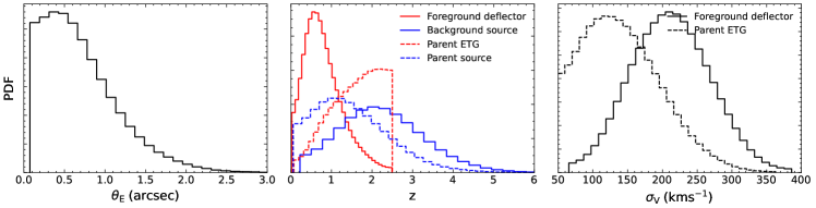
Figure 1: Population statistics of the ideal strong lens sample. Left panel: the probability density distribution of the Einstein radius. Middle panel: the redshift probability distribution. The red and blue histograms represent the redshift distributions of the foreground lens and the background source, respectively; while the red and the blue dashed lines represent the original redshift distributions of the ETGs and the source galaxies used to simulate strong lenses, respectively. Right panel: the velocity dispersion distribution of the lens galaxy.

3.1 Ideal lens sample

Based on the ETG population described in Section 2.1.1, our prediction suggests that the sky harbors approximately 2.1 billion ETGs within the redshift range of 0 to 2.5. Subsequently, with the introduction of the source population discussed in Section 2.1.2, approximately 12 million of these ETGs act as deflectors, exerting a strong lensing effect on the background source. The rate of strong lensing is estimated to be around 0.6%. Figure 1 depicts the population properties of the ideal lens sample. The left panel displays the probability density distribution of the lensing Einstein radius, peaking at approximately 0.5$\arcsec$, with a tail extending to $3.0\arcsec$. In the middle panel, the red solid line signifies the redshift probability density distribution of the lens galaxies, whereas the blue solid line represents the distribution of the source galaxies. The lens galaxies display a median redshift of approximately 0.71. The red and blue dashed lines correspond to the redshift distributions of the original ETGs and sources used for lensing simulation, respectively. In this work, we manually truncate the redshift distribution of the original ETGs at 2.5. Considering the scarcity of lensing objects with redshifts near 2.5 in the ideal lens sample (as evident from the red solid line), this choice does not lead to a significant underestimation of the forecasted number of lens samples, at least concerning the source catalog employed in this study. The solid line in the right panel shows the probability density distribution of the velocity dispersion for the lens galaxy, having a median of $210.53\pm 52.34\,\text{km/s}$; the dashed line shows the parent galaxy sample. It is worth noting that our Figure 1 is in agreement with the results presented in Collett (2015), thereby validating the simulation code utilized in this work.

3.2 CSST lens sample

The CSST survey comprises three operational modes: the “Wide Field” (WF), the “Deep Field” (DF), and the “Ultra Deep Field” (UDF). The WF mode covers a sky area of 17,500 square degrees with a $300\,s$ exposure time. In contrast, the DF mode uses a longer exposure time of $2000\,s$ but covers a smaller survey area of 400 square degrees. Additionally, the UDF mode aims to achieve a similar scientific goal as the well-known Hubble Ultra-Deep Field by targeting a sky area of 9 square degrees with an exposure time of $15000\,s$. Sections 3.2.1, 3.2.2, and 3.2.3 present the GGSLs of CSST under the WF, DF, and UDF surveys, respectively.

3.2.1 Wide-field lens sample

If the condition for identifying a strong lens is to satisfy the "detection requirements" outlined in Section 2.3 in at least one image from the $g$, $r$, $i$, or $z$ bands, we can identify approximately 76,000 strong lenses in CSST WF mode. Among these, approximately 41,000 display extended arc structures. It turns out that the lensed features are most prominently detected in the $g$ band, with approximately 78% of lenses identified through the single-band image exhibiting the highest SNR in the $g$ band. This can be attributed to the fact that high redshift sources often experience star formation and exhibit a bluer color compared to the redder early-type lens galaxies. We refer to this strong lens sample as the "single-band" one. Roughly 96% of the strong lenses in the ideal lens sample did not meet the criteria to be classified as part of the single-band sample due to their failure to satisfy the arc SNR condition outlined in Section 2.3. However, if we sacrifice the color information and stack the images from the $g$, $r$, $i$, and $z$ bands to enhance the arc SNR, the number of detectable strong lenses will increase to approximately 160,000 with around 82,000 having the extended arc structure. This set of lenses is referred to as the "stacked" sample. Our lensing simulation shows that the SNR of the lensed images varies between approximately 20 and 1000 in the stacked sample (refer to the left panel of Figure 3). Among these lenses, approximately 4,000 exhibit bright lensed images with $\rm SNR_{\rm arc}>100$, making them of particular interest as they provide better constraints on the lens’s mass (see Section 4), thus forming the "golden sample." To provide an intuitive demonstration, Figure 2 shows three example lenses from the stacked sample that possess relatively faint lensed images (top row, $\rm SNR_{\rm arc}\approx 20$), bright lensed images (middle row, $\rm SNR_{\rm arc}\approx 100$), and small Einstein radius (bottom row, $\rm\theta_{\rm E}\approx 0.08$), respectively.

Figure 4 presents the population properties of the strong lens sample under the CSST WF mode, employing both the "stacked" (solid lines) and "single band" (dashed lines) detection criteria. In the top left panel, the blue and red lines show how the number of strong lenses varies with the lens and source redshift, respectively. The vertical dotted line indicates the redshift of 1. In the top right, bottom left, and bottom right panels: histograms show the distribution of the Einstein mass, total magnification, and intrinsic (unlensed) source magnitude. The Einstein mass of deflectors spans from $1.47\times 10^{9}M_{\odot}$ to $1.97\times 10^{12}M_{\odot}$, with a median value of approximately $1.36\times 10^{11}M_{\odot}$. Around $40\%$ of the CSST WF samples have an Einstein mass smaller than $10^{11}M_{\odot}$, as indicated by the vertical dotted line in the top-right panel. This significantly enhances the completeness of the sample for strong lenses in the low-mass range. The total magnification has a median value around $\sim 5$ and exhibits a high-magnification long tail extending to values around 100. Moreover, the intrinsic (or unlensed) g-band apparent magnitude of the source exhibits median values of approximately 25.40 and 25.87 for the “stacked” and “single-band” samples, respectively, as illustrated by the vertical lines in the bottom-right panel.

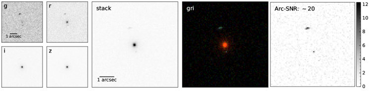
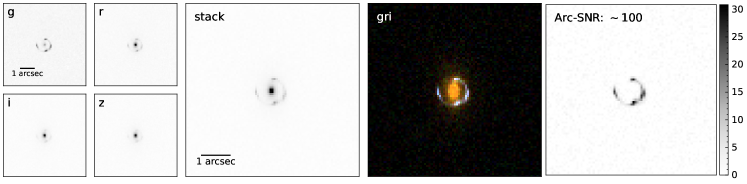
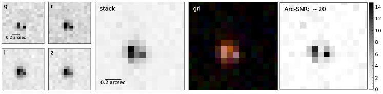
Figure 2: Three lens systems with relatively faint ($\rm SNR_{\rm arc}\approx 20$) lensed images, bright ($\rm SNR_{\rm arc}\approx 100$) lensed images, and small Einstein radius ($\theta_{\rm E}\approx 0.08$) are shown at the top, middle, and bottom rows, respectively. In each row, the left panels show separate images in the $g$, $r$, $i$, and $z$ bands. The middle-left panel displays the stacked image that combines the $g$, $r$, $i$, and $z$ bands. The middle-right panel presents the composite color image. The right panel exhibits the SNR map of the lensed arc for the stacked image.

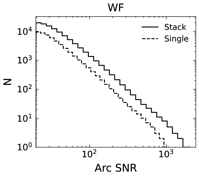
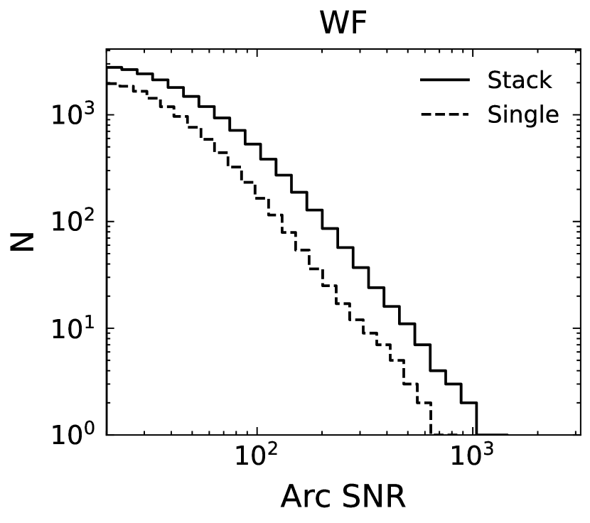
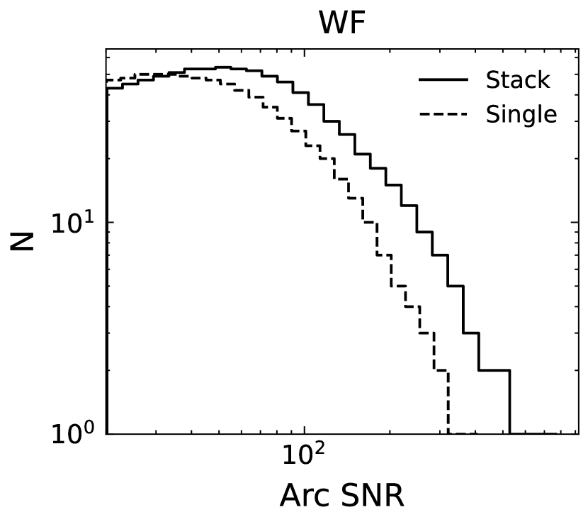
Figure 3: The histograms show the distribution of arc SNR for the wide field (left panel), deep field (middle panel), and ultra-deep field (right panel) surveys. Arc SNR measurements come from either the stacked image (solid lines) or the single-band image with the highest arc SNR (dashed lines).

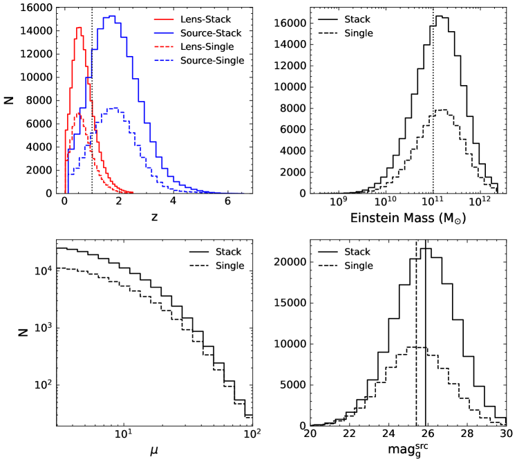
Figure 4: Population statistics of the CSST strong lens sample. Top left panel: The red line shows the number of lens galaxies, and the blue line shows the number of sources as a function of redshift. Solid lines represent the lens samples detected via the stacked image, while the dashed lines correspond to those detected using the single-band image with the highest arc signal-to-noise ratio (SNR). Top right, bottom left, and bottom right panels: The histograms show the distribution of the Einstein mass, total magnification, and intrinsic (unlensed) source magnitude at the g band for both the "stacked" (solid lines) and "single band" (dashed lines) samples.

3.2.2 Deep-field lens sample

Under the "single-band" detection criteria, a search in the CSST DF mode image data yields around $\sim 12,000$ lenses, of which approximately $\sim 5000$ exhibit extended arc structures. Employing the "stacked" detection scheme results in an increase to approximately $\sim 17,900$ and $\sim 7300$ for these two respective numbers. The middle panel of Figure 3 shows the number distribution of lenses with respect to the arc SNR. Other lensing properties (redshift, Einstein radius, magnification, etc) of the lens sample under the CSST DF mode are not significantly different from those of the WF mode. However, the median intrinsic $g$-band source magnitude is approximately $0.98$ magnitude deeper in the DF mode, attributable to the longer exposure time.

3.2.3 Ultra-Deep-Field lens sample

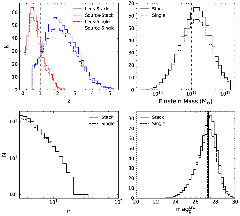
Figure 11: Similar to Figure 4, but for the CSST ultra-deep field surveys.

The CSST UDF survey has the capability to identify $\sim 730$ strong lenses employing the "single band" detection approach and $\sim 840$ lenses using the "stacked" detection scheme. Within this set, $\sim 280$ lenses showcase an extended arc structure under the "single band" criterion, whereas $\sim 320$ lenses exhibit this feature through the "stacked" approach. The distribution of arc SNR is illustrated in the right panel of Figure 3, while various lensing properties are shown in Figure 11. Particularly noteworthy, the median $g$-band magnitude of the source in the UDF mode is approximately $0.44$ magnitude deeper compared to the DF mode.

3.3 Comparing lens samples from different surveys

In the upcoming decade, the landscape of optical-band image surveys will be shaped by prominent projects such as CSST, Euclid, and LSST. Both CSST and Euclid are space telescopes, offering a distinct advantage in spatial resolution compared to their ground-based counterparts like LSST. Conversely, the LSST holds considerable promise for facilitating time-domain studies. To enable a comprehensive comparative analysis of lens samples across these three image surveys, we acquire the lensing sample predictions for LSST directly from Collett (2015). Subsequently, we conduct a new lensing simulation tailored to the Euclid survey, employing the latest instrument settings outlined in Table 1. The resulting comparison is visually depicted in Figure 5, illustrating the distribution of lenses relative to both the Einstein radius (left panel) and velocity dispersion (right panel). The black histogram represents the results from the CSST WF mode, using the “stacked” detection scheme. The red histogram represents the one from the Euclid survey by searching strong lenses in the $VIS$ band image. The blue histogram shows the lens sample distribution from the LSST survey, using the “optimal stacked” scheme for lens searching Collett (2015). CSST, Euclid, and LSST are forecasted to detect approximately 160000, 132000, and 129000 lenses, respectively. The velocity dispersion of the CSST lens sample is $217.19\pm 50.55\,\text{km/s}$ (median$\pm$standard deviation) similar to that from Euclid’s result, $221.10\pm 48.18\,\text{km/s}$. The lens sample of CSST exhibits Einstein radii of $0.64\pm 0.43\arcsec$, slightly smaller than Euclid’s $0.66\pm 0.40\arcsec$. However, these values remain comparable, suggesting that the two surveys have similar lens populations. LSST lenses show a velocity dispersion of $258.09\pm 41.62\,{km/s}$ and an Einstein radius of $1.14\pm 0.42\arcsec$; thus, its selection function favors more massive lenses.

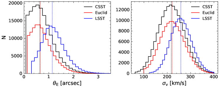
Figure 5: The number distribution of the lens sample as a function of the Einstein radius (left panel) and the velocity dispersion (right panel), for the CSST (black lines), the LSST (blue lines), and the Euclid (red lines) survey. In comparison to the ground-based LSST, CSST and Euclid can detect a larger number of lenses with smaller Einstein radii and lower velocity dispersions, which correspond to ETGs with lower masses. The vertical dotted lines indicate the median values of each distribution.

4 Summary and Discussion

In this paper, we performed a Monte Carlo simulation which adopts a realistic population for the lens and source properties, to predict how many GGSLs would be observed by CSST and explore the population statistics of those CSST lenses. our simulations consider various selection functions, including the telescope PSF, the survey depth, and the lensing magnification bias (Kochanek, 2004).

We find that the CSST has the potential to discover approximately 160,000 GGSLs through the wide-field survey using the "stacked image", assuming a Poisson-limited lens light subtraction. The number of lenses reduces to approximately 17,900 and 840 for the CSST deep-field and ultra-deep-field surveys, respectively. By imposing the condition that the lensing feature must be detected in at least one of the individual $g$, $r$, $i$, and $z$ bands, the CSST wide-field, deep-field, and ultra-deep-field surveys would detect approximately 76,400, 12,000, and 730 GGSLs, respectively. To facilitate the reader’s accessibility, we compile the information on the number of detectable lenses for CSST in Table 2.

Figure 6: Lens modeling accuracy with respect to the Einstein radius in relation to the total SNR of the lensed arc is explored. The SNR range, spanning from 20 to 1000, is divided into six equally spaced logarithmic bins, each containing 30 lenses with diverse lensing configurations. The median modeling accuracy is indicated by black dots within each SNR bin. This accuracy accounts for both biases and statistical uncertainties. Notably, the modeling accuracy in the highest SNR bins shows a slight degradation, attributed to the more pronounced adverse impact of the imperfect PSF for the stacked image.

For gravitational lenses identified through the CSST wide-field survey using stacked images, the SNR of the lensed arcs varies from $\sim 20$ to $\sim 1000$. To assess the precision with which the lensed arc can constrain the lens mass model, we model the lensed arc images generated by our lensing simulation with an SIE lens plus Sersic source model, assuming the lens light has been subtracted to the noise level. We find the Einstein radius can be pinned down to $\sim 1\%$ and $\sim 0.1\%$ levels (see Figure 6), depending on the SNR of the lensed arc. There is a counter-intuitive trend where the modeling accuracy deteriorates for the highest SNR bin. We attribute this to the presence of an imperfect PSF in the stacked image, as the PSF size is oversimplified by taking the mean FWHM across the $g$, $r$, $i$, and $z$ bands. Future analyses can circumvent this issue by directly performing multi-band lens modeling instead of working on the stacked image. This will mitigate the impact of an imperfect PSF while preserving the SNR enhancement provided by multi-band data. It is important to note that the reported precisions here do not account for various systematic effects that can affect the accuracy of lens modeling, such as missing complexities in the mass model (Cao et al., 2022; He et al., 2023a; Van de Vyvere et al., 2022a, b; Etherington et al., 2023; O’Riordan & Vegetti, 2023; Du et al., 2023), inaccurate PSF (Shajib et al., 2022), imperfect subtraction of the lens light (Nightingale et al., 2022), and correlated CCD noise when working with real lens data. Nevertheless, these values provide insights into the statistical ability of lensed arcs to constrain the mass of the lens.

Among those $\sim$160,000 CSST lenses, some systems that are either rare or undetected in previous lens samples, such as high-redshift ($z_{l}>1$) or low-mass ($M_{ein}<10^{11}M_{\odot}$), draw particular interest since they represent “place in parameter space” that are uncovered by the current sample. Our simulations predict the CSST could find $\sim$31000 high-redshift and $\sim$62000 low-mass lenses, significantly increasing the completeness of the GGSL sample. Furthermore, CSST has the potential to detect unusual systems such as spiral galaxy lenses and double source-plane lenses. Regarding spiral galaxy lenses, estimating them accurately is a complex task that requires the development of a dedicated population model specific to spiral galaxies. Although constructing such a model exceeds the scope of this study, it is possible to provide a rough estimate of the number of spiral galaxy lenses by considering the proportion of existing spiral galaxy lenses. For instance, the SLACS project identified approximately $\sim 10\%$ (10 out of 85) of GGSLs as spiral galaxy lenses. By extrapolating this ratio, it is plausible to suggest that the CSST could potentially detect around $\sim 15,000$ spiral galaxy lenses. In the case of double source-plane lenses, where two sources located at different redshifts generate distinct images, these systems play a crucial role in mitigating the mass-sheet degeneracy that complicates lens modeling and provides valuable constraints on cosmological parameters. Sharma et al. (2023) predicts that the Euclid survey could discover around 1700 double source-plane lenses. Given the similar depth and spatial resolution between the CSST and Euclid, we anticipate that the CSST wide-field survey could identify around 1,500 such instances.

Table 2: We present the number of detectable lenses using various detection schemes. These schemes utilize single-band images (referred to as "single"), stacked images (referred to as "stack"), or a combination of both (referred to as "combine"), and are categorized under various CSST survey modes (WF, DF, and UDF). Additionally, we provide the number of lenses that exhibit bright lensed images (with $\rm SNR_{\rm arc}>100$), have a redshift exceeding 1, and possess an Einstein mass lower than $10^{11}M_{\odot}$.

	WF	DF	UDF
stack	161548	17877	836
single	76396	11951	728
combine	162584	18183	847
$\rm SNR_{\rm arc}>100$	4079	1019	201
$z_{l}>1$	30695	4242	208
$M_{ein}<10^{11}M_{\odot}$	61591	6936	312

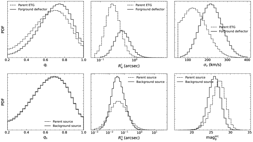
Figure 7: This figure illustrates the lensing selection effect through a comparative analysis of the properties of the lens sample and its parent population. The top panels, from left to right, show solid lines representing the probability density functions (PDFs) of the lens galaxy’s axis ratio, effective radius, and velocity dispersion, while the corresponding parent population PDFs are shown by the dashed lines. Moving to the bottom panels, from left to right, we compare differences in the PDFs between the lens and parent populations for the source’s axis ratio, effective radius, and g-band magnitude.

While the number of CSST lenses is of interest, understanding the selection effects inherent to CSST GGSL observations is also crucial. Figure 7 presents the probability density distribution of various lensing properties, for both lens (solid lines) and parent population (dashed lines). The top panels reveal that ETGs acting as lenses is typically larger, both in terms of mass (evidenced by velocity dispersion) and observable size (manifested by effective radius). Additionally, lens ETGs tend to be rounder, consistent with findings from other lensing works. The lower panels highlight that lensed sources tend to exhibit higher luminosity compared to the parent sample, attributable to the depth limitations of CSST. Unlike the lens galaxies, the source exhibits no substantial axis-ratio selection effect. The size distribution of lensed sources peaks around $\sim 0.09\arcsec$, displaying fewer instances of both exceptionally small and larger sources in comparison to the parent sample. This outcome emerges from the interplay of two distinct factors. When the source size is exceptionally small, it also typically manifests faintness in line with the applied scaling relation (see equation 5). Consequently, the lensed arc lacks the requisite SNR for successful detection. Conversely, if the source size is markedly large, it fails to meet the criteria for “resolved condition” illustrated in Section 2.3, leading to the incapacity to identify counter images produced by the strong lensing.

The major source of uncertainties that could significantly change the number of GGSLs predicted by our simulation is the choice of lens finder, as demonstrated by Collett (2015). In this work, we have deliberately adopted the same detectability condition as Collett (2015) (thus the same lens finder), for a consistent comparison. These detectability conditions are proved to be reasonably good by visually inspecting the lensing image. Nevertheless, we still try three different choices to tighten the detection criteria for a more thorough investigation. We raise the SNR threshold from 20 to 40, increase the magnification threshold from 3 to 4, and modify the image-resolved threshold from $\theta_{\mathrm{E}}^{2}>(R_{\rm e}^{s})^{2}+(s/2)^{2}$ to $\theta_{\mathrm{E}}^{2}>(R_{\rm e}^{s})^{2}+s^{2}$. We find the number of detectable lens drops by 77%, 26%, and 2%, respectively; While the change in arc SNR is the primary factor that affects the number of detectable lenses. Visually inspecting the lens-light subtracted image shows the lensed features are already evident when the total arc SNR reaches 20.

Our simulations reveal that the population statistics of CSST and Euclid strong lenses are similar, which is expected considering their similar spatial resolution and depth. However, the smaller PSF and pixel sizes of CSST provide it with certain advantages in the detection of small-mass lenses. As both telescopes cover nearly identical sky regions, it is crucial to effectively coordinate the use of GGSLs data from these two surveys. In the future, CSST and Euclid will discover hundreds of thousands of strong lenses, making the acquisition of their spectroscopic redshifts costly. Unlike Euclid, CSST possesses optical color information ($ugriz$), which allows for the calculation of lens/source galaxy photometric redshifts. However, CSST’s lack of infrared photometric information significantly hampers the photometric redshift accuracy of high-redshift source galaxies ($z>1$); Euclid’s NIR infrared band information can mitigate this limitation. Additionally, a joint analysis using CSST and Euclid’s image data can be conducted. This approach is somewhat akin to stacking images from two separate surveys to enhance the signal-to-noise ratio, which in turn leads to more robust constraints on lens models.

Data Availability

The code and data product that supports this work is publicly available from https://github.com/caoxiaoyue/sim_csst_lens.

Appendix A The FWHM of CSST’s PSF

The CSST employs the $R_{\mathrm{EE80}}$ as the primary metric for defining the properties of the PSF, whereas other telescopes like HST and Euclid typically use the FWHM. To enable a direct comparison between different telescopes, we determine the FWHM by fitting a Gaussian model to a set of simulated PSF images captured by the CSST. Figure 8 shows an example of PSF fitting in the $i$ band. Figure 9 presents the distribution of PSF FWHM in the $i$ band, illustrating the slight variation in PSF size across the CCD focal plane. The reported FWHM value of the PSF in Table 1 corresponds to the median.

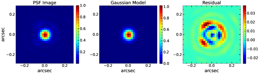
Figure 8: To obtain the FWHM value, a Gaussian model is employed to fit the simulated PSF image of CSST. Panels from left to right display the simulated PSF image, the image obtained through Gaussian model fitting, and the residual image calculated as the difference between the left and middle panels. Images shown here have a 4 by 4 supersampling, resulting in a pixel size of $0.074/4=0.0185\arcsec$.

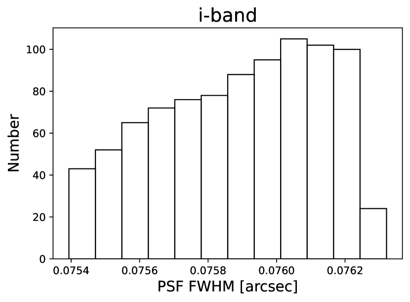
Figure 9: The distribution of FWHM values for the PSF of CSST in the $i$ band. The variation in PSF size is caused by changes in position within the CCD focal plane.

For a comprehensive crosscheck, we also attempted to apply Gaussian model fitting to an HST PSF in the F814W filters. The resulting FWHM value was approximately $0.09\arcsec$, which closely resembles that of the CSST $z$ band ($\sim 0.089\arcsec$). This result aligns with our expectations, as both the HST and CSST are two-meter telescopes, and the F814W filters closely correspond to the CSST $z$ band in terms of wavelength.

Appendix B Other lensing properties

The population statistics of the lens sample for the CSST deep field and ultra-deep field surveys are presented in Figures 10 and  11, respectively.

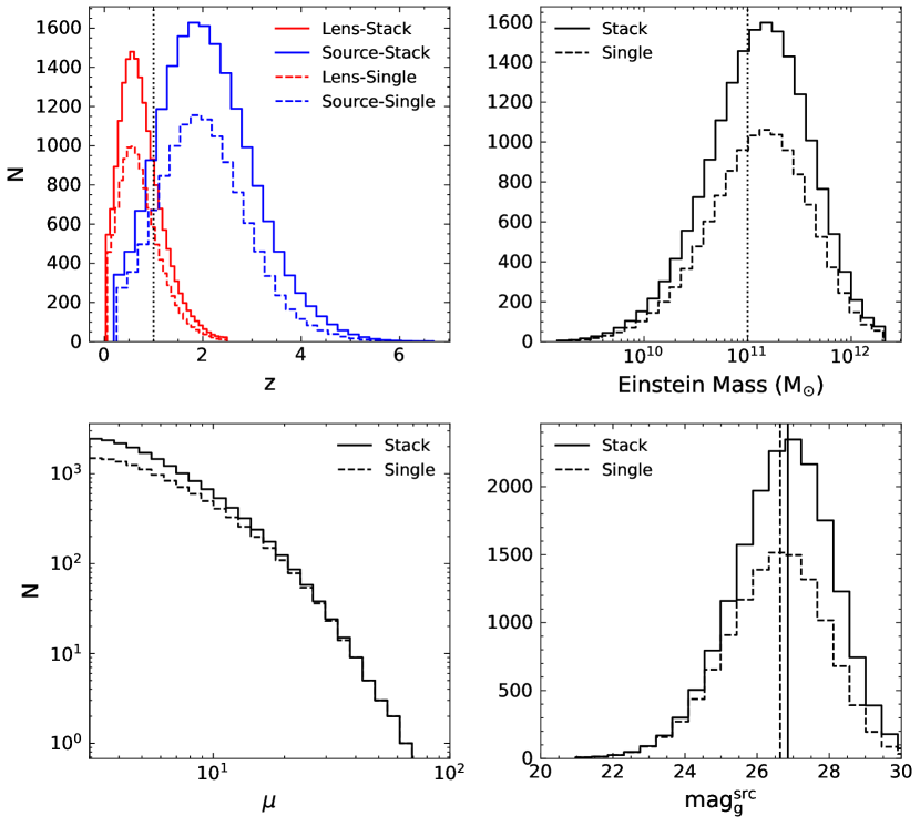
Figure 10: Similar to Figure 4, but for the CSST deep field surveys.

Appendix C Remark on the depth of CSST and Euclid

The CSST boasts a telescope diameter of two meters, giving it a significant advantage in terms of depth when compared to Euclid, which has a smaller one-meter diameter. However, it’s worth noting that Euclid compensates for its smaller size with longer exposure times of $565\times 3$s for its wide field survey, whereas CSST employs shorter exposure times of $150\times 2$s. Moreover, the $VIS$ imager on Euclid is equipped with a broad-band filter that effectively covers the $riz$ bands present in CSST. As a result, making an apple-to-apple comparison between the two telescopes becomes somewhat indirect due to these contrasting factors. We shall consider two examples here to illustrate the depth of CSST and Euclid, in particular for our lensing simulation.

To begin, let’s consider a source exhibiting an apparent magnitude of 25 in the $riz$ bands. According to the approximation outlined in Collett (2015), the magnitude in the $VIS$ band is also 25, as it represents the mean of the $riz$ bands. Consequently, CSST’s 300s exposures will generate 1823 electron count on the CCD, whereas Euclid, with a longer exposure time of 1695s, will generate 2092 electron counts. With a higher number of electron counts, Euclid shows a larger signal-to-noise ratio, taking into account the Poisson noise. Thus, in terms of the $VIS$ band, Euclid’s wide-field survey offers slightly greater depth compared to CSST’s.

Next, let us explore the appearance of observable lenses in our CSST lensing simulation within the context of the Euclid survey. Figure 12 presents a typical example illustrating this comparison. The panels, arranged from top-left to bottom-right, depict the ideal SNR maps of the lensed arc (representing the noise map prior to incorporating a noise realization) for CSST-$g$, CSST-$r$, CSST-$i$, CCSST-$z$, CSST-$stack$, and Euclid $VIS$ bands, respectively. The legend provides the total SNR values corresponding to the lensed arc. Remarkably, our analysis indicates that CSST and Euclid yield similar depths in terms of the detected total SNR of the lensed arc. However, CSST exhibits a slightly higher SNR value, indicating a better depth of observation. This advantage arises from the stacking of images from the $g$, $r$, $i$, and $z$ bands, as well as the smaller PSF of CSST that results in sharper images.

It is important to note that our CSST lensing simulation solely incorporates the $griz$ bands. This limitation arises from the fact that the source catalog we utilized currently lacks data from other bands. However, it is worth considering that by stacking the image data from the $u$ and $NUV$ bands, we may potentially enhance the number of detectable lenses within CSST.

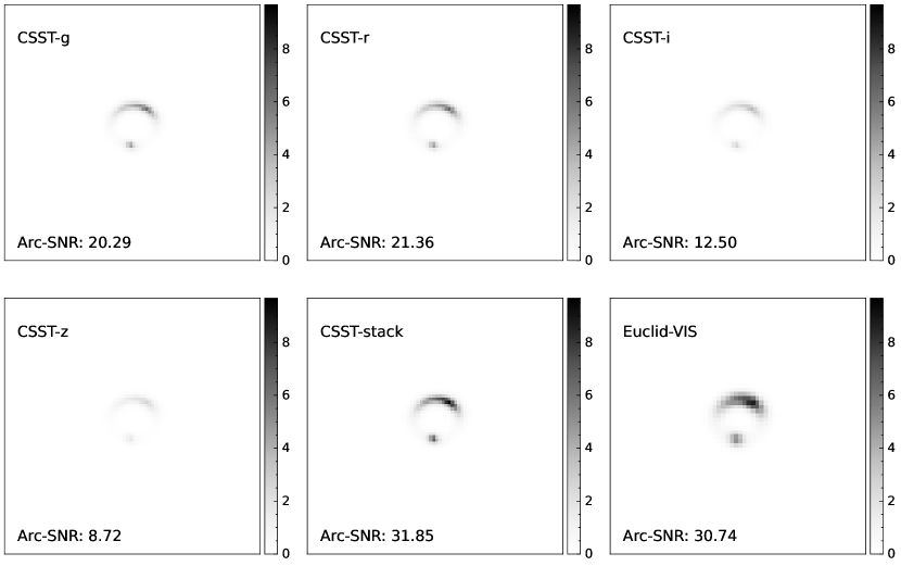
Figure 12: The ideal signal-to-noise ratio (SNR) map of the lensed arc is generated without noise realization. It is computed for the CSST filters $g$, $r$, $i$, $z$, the stack image of $griz$, and the Euclid $VIS$ image. The total SNR of the lensed arc is provided in the legend for each filter.

Appendix D Lens modeling results

The lensed images generated by our lensing simulation, after subtracting the lens light, are modeled using an SIE lens plus a Sersic source model. The modeling results for several example lenses are arranged in rows from top to bottom in Figure 13, based on the SNR of the lensed images. Each row consists of three panels displaying the modeling results of three example lenses. These lenses have similar SNR levels but different lensing geometries, with the data and model images shown on the left and right, respectively.

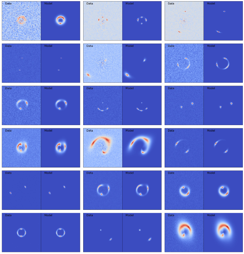
Figure 13: From top to bottom rows, the SNR of the lensed images is at the level of approximately 28, 53, 102, 196, 376, and 722, corresponding to the six equally spaced logarithmic bins employed in Figure 6. Each row contains three panels displaying the lens modeling results of three lenses with distinct lensing geometries. The data and model images are shown on the left and right, respectively.

References

- Aihara et al. (2018) Aihara H., et al., 2018, PASJ, 70, S8
- Auger et al. (2009) Auger M. W., Treu T., Bolton A. S., Gavazzi R., Koopmans L. V. E., Marshall P. J., Bundy K., Moustakas L. A., 2009, ApJ, 705, 1099
- Auger et al. (2010) Auger M. W., Treu T., Bolton A. S., Gavazzi R., Koopmans L. V. E., Marshall P. J., Moustakas L. A., Burles S., 2010, ApJ, 724, 511
- Bayer et al. (2023) Bayer D., Chatterjee S., Koopmans L. V. E., Vegetti S., McKean J. P., Treu T., Fassnacht C. D., Glazebrook K., 2023, MNRAS, 523, 1310
- Bezanson et al. (2011) Bezanson R., et al., 2011, ApJ, 737, L31
- Birrer et al. (2020) Birrer S., et al., 2020, A&A, 643, A165
- Blecher et al. (2019) Blecher T., Deane R., Heywood I., Obreschkow D., 2019, MNRAS, 484, 3681
- Bolton et al. (2006) Bolton A. S., Rappaport S., Burles S., 2006, Phys. Rev. D, 74, 061501
- Bolton et al. (2008) Bolton A. S., Treu T., Koopmans L. V. E., Gavazzi R., Moustakas L. A., Burles S., Schlegel D. J., Wayth R., 2008, ApJ, 684, 248
- Bolton et al. (2012) Bolton A. S., et al., 2012, ApJ, 757, 82
- Cañameras et al. (2021) Cañameras R., et al., 2021, A&A, 653, L6
- Cao et al. (2017) Cao S., Li X., Biesiada M., Xu T., Cai Y., Zhu Z.-H., 2017, ApJ, 835, 92
- Cao et al. (2022) Cao X., et al., 2022, Research in Astronomy and Astrophysics, 22, 025014
- Chakraborty & Roy (2023) Chakraborty A., Roy N., 2023, MNRAS, 519, 4074
- Chan et al. (2020) Chan J. H. H., et al., 2020, A&A, 636, A87
- Chang et al. (2015) Chang C., et al., 2015, ApJ, 801, 73
- Chen et al. (2019) Chen Y., Li R., Shu Y., Cao X., 2019, MNRAS, 488, 3745
- Cheng et al. (2020) Cheng C., et al., 2020, ApJ, 898, 33
- Choi et al. (2007) Choi Y.-Y., Park C., Vogeley M. S., 2007, ApJ, 658, 884
- Collett (2015) Collett T. E., 2015, ApJ, 811, 20
- Collett & Auger (2014) Collett T. E., Auger M. W., 2014, MNRAS, 443, 969
- Collett et al. (2018) Collett T. E., et al., 2018, Science, 360, 1342
- Collett et al. (2023) Collett T. E., et al., 2023, The Messenger, 190, 49
- Connolly et al. (2010) Connolly A. J., et al., 2010, in Angeli G. Z., Dierickx P., eds, Society of Photo-Optical Instrumentation Engineers (SPIE) Conference Series Vol. 7738, Modeling, Systems Engineering, and Project Management for Astronomy IV. p. 77381O, doi:10.1117/12.857819
- Cornachione et al. (2018) Cornachione M. A., et al., 2018, ApJ, 853, 148
- Cropper et al. (2016) Cropper M., et al., 2016, in MacEwen H. A., Fazio G. G., Lystrup M., Batalha N., Siegler N., Tong E. C., eds, Society of Photo-Optical Instrumentation Engineers (SPIE) Conference Series Vol. 9904, Space Telescopes and Instrumentation 2016: Optical, Infrared, and Millimeter Wave. p. 99040Q (arXiv:1608.08603), doi:10.1117/12.2234739
- Dey et al. (2019) Dey A., et al., 2019, AJ, 157, 168
- Du et al. (2020) Du W., Zhao G.-B., Fan Z., Shu Y., Li R., Mao S., 2020, ApJ, 892, 62
- Du et al. (2023) Du W., Fu L., Shu Y., Li R., Fan Z., Shu C., 2023, ApJ, 953, 189
- Enzi et al. (2020) Enzi W., Vegetti S., Despali G., Hsueh J.-W., Metcalf R. B., 2020, MNRAS, 496, 1718
- Etherington et al. (2023) Etherington A., et al., 2023, arXiv e-prints, p. arXiv:2301.05244
- Euclid Collaboration et al. (2019) Euclid Collaboration et al., 2019, A&A, 627, A59
- Euclid Collaboration et al. (2022) Euclid Collaboration et al., 2022, A&A, 662, A112
- Gavazzi et al. (2007) Gavazzi R., Treu T., Rhodes J. D., Koopmans L. V. E., Bolton A. S., Burles S., Massey R. J., Moustakas L. A., 2007, ApJ, 667, 176
- Geng et al. (2021) Geng S., Cao S., Liu Y., Liu T., Biesiada M., Lian Y., 2021, MNRAS, 503, 1319
- Gilman et al. (2019) Gilman D., Birrer S., Treu T., Nierenberg A., Benson A., 2019, MNRAS, 487, 5721
- Gilman et al. (2020) Gilman D., Birrer S., Nierenberg A., Treu T., Du X., Benson A., 2020, MNRAS, 491, 6077
- He et al. (2018) He Q., Li R., Lim S., Frenk C. S., Cole S., Peng E. W., Wang Q., 2018, MNRAS, 480, 5084
- He et al. (2020a) He Q., et al., 2020a, arXiv e-prints, p. arXiv:2010.13221
- He et al. (2020b) He Q., et al., 2020b, MNRAS, 496, 4717
- He et al. (2023a) He Q., et al., 2023a, MNRAS, 518, 220
- He et al. (2023b) He Z., Li N., Cao X., Li R., Zou H., Dye S., 2023b, A&A, 672, A123
- Huang et al. (2021) Huang X., et al., 2021, ApJ, 909, 27
- Hyde & Bernardi (2009) Hyde J. B., Bernardi M., 2009, MNRAS, 396, 1171
- Jacobs et al. (2019) Jacobs C., et al., 2019, MNRAS, 484, 5330
- Kochanek (2004) Kochanek C. S., 2004, arXiv preprint astro-ph/0407232
- Koopmans et al. (2006) Koopmans L. V. E., Treu T., Bolton A. S., Burles S., Moustakas L. A., 2006, ApJ, 649, 599
- Kormann et al. (1994) Kormann R., Schneider P., Bartelmann M., 1994, A&A, 284, 285
- Li et al. (2016) Li R., Frenk C. S., Cole S., Gao L., Bose S., Hellwing W. A., 2016, MNRAS, 460, 363
- Li et al. (2017) Li R., Frenk C. S., Cole S., Wang Q., Gao L., 2017, MNRAS, 468, 1426
- Li et al. (2021) Li R., et al., 2021, ApJ, 923, 16
- Magee et al. (2023) Magee M. R., Sainz de Murieta A., Collett T. E., Enzi W., 2023, arXiv e-prints, p. arXiv:2303.15439
- Mao & Schneider (1998) Mao S., Schneider P., 1998, MNRAS, 295, 587
- Marques-Chaves et al. (2020) Marques-Chaves R., et al., 2020, MNRAS, 499, L105
- Millon et al. (2020) Millon M., et al., 2020, A&A, 639, A101
- Möller et al. (2007) Möller O., Kitzbichler M., Natarajan P., 2007, MNRAS, 379, 1195
- Napolitano et al. (2016) Napolitano N. R., et al., 2016, in Napolitano N. R., Longo G., Marconi M., Paolillo M., Iodice E., eds, Astrophysics and Space Science Proceedings Vol. 42, The Universe of Digital Sky Surveys. p. 129 (arXiv:1507.00733), doi:10.1007/978-3-319-19330-4_20
- Newton et al. (2011) Newton E. R., Marshall P. J., Treu T., Auger M. W., Gavazzi R., Bolton A. S., Koopmans L. V. E., Moustakas L. A., 2011, ApJ, 734, 104
- Nightingale et al. (2019) Nightingale J. W., Massey R. J., Harvey D. R., Cooper A. P., Etherington A., Tam S.-I., Hayes R. G., 2019, MNRAS, 489, 2049
- Nightingale et al. (2022) Nightingale J. W., et al., 2022, arXiv e-prints, p. arXiv:2209.10566
- O’Riordan & Vegetti (2023) O’Riordan C. M., Vegetti S., 2023, arXiv e-prints, p. arXiv:2310.10714
- Oguri et al. (2012) Oguri M., et al., 2012, AJ, 143, 120
- Petrillo et al. (2019) Petrillo C. E., et al., 2019, MNRAS, 484, 3879
- Planck Collaboration et al. (2016) Planck Collaboration et al., 2016, A&A, 594, A13
- Pohlen & Trujillo (2006) Pohlen M., Trujillo I., 2006, A&A, 454, 759
- Ritondale et al. (2019a) Ritondale E., Auger M. W., Vegetti S., McKean J. P., 2019a, MNRAS, 482, 4744
- Ritondale et al. (2019b) Ritondale E., Vegetti S., Despali G., Auger M. W., Koopmans L. V. E., McKean J. P., 2019b, MNRAS, 485, 2179
- Rizzo et al. (2020) Rizzo F., Vegetti S., Powell D., Fraternali F., McKean J. P., Stacey H. R., White S. D. M., 2020, Nature, 584, 201
- Sérsic (1963) Sérsic J. L., 1963, Boletin de la Asociacion Argentina de Astronomia La Plata Argentina, 6, 41
- Shajib et al. (2022) Shajib A. J., et al., 2022, A&A, 667, A123
- Sharma et al. (2023) Sharma D., Collett T. E., Linder E. V., 2023, J. Cosmology Astropart. Phys., 2023, 001
- Sheu et al. (2023) Sheu W., Huang X., Cikota A., Suzuki N., Schlegel D., Storfer C., 2023, arXiv e-prints, p. arXiv:2301.03578
- Shu et al. (2015) Shu Y., et al., 2015, ApJ, 803, 71
- Shu et al. (2016) Shu Y., et al., 2016, ApJ, 833, 264
- Shu et al. (2017) Shu Y., et al., 2017, ApJ, 851, 48
- Shu et al. (2022) Shu Y., Cañameras R., Schuldt S., Suyu S. H., Taubenberger S., Inoue K. T., Jaelani A. T., 2022, A&A, 662, A4
- Sonnenfeld (2021) Sonnenfeld A., 2021, A&A, 656, A153
- Sonnenfeld (2022) Sonnenfeld A., 2022, A&A, 659, A132
- Sonnenfeld & Cautun (2021) Sonnenfeld A., Cautun M., 2021, A&A, 651, A18
- Sonnenfeld et al. (2018) Sonnenfeld A., et al., 2018, PASJ, 70, S29
- Storfer et al. (2022) Storfer C., et al., 2022, arXiv e-prints, p. arXiv:2206.02764
- Suyu et al. (2013) Suyu S. H., et al., 2013, ApJ, 766, 70
- Suyu et al. (2023) Suyu S. H., Goobar A., Collett T., More A., Vernardos G., 2023, arXiv e-prints, p. arXiv:2301.07729
- Taylor et al. (2022) Taylor L., et al., 2022, ApJ, 939, 90
- Treu et al. (2006) Treu T., Koopmans L. V., Bolton A. S., Burles S., Moustakas L. A., 2006, ApJ, 640, 662
- Treu et al. (2022) Treu T., Suyu S. H., Marshall P. J., 2022, A&ARv, 30, 8
- Van de Vyvere et al. (2022a) Van de Vyvere L., Gomer M. R., Sluse D., Xu D., Birrer S., Galan A., Vernardos G., 2022a, Astron. Astrophys., 659, A127
- Van de Vyvere et al. (2022b) Van de Vyvere L., Sluse D., Gomer M. R., Mukherjee S., 2022b, Astron. Astrophys., 663, A179
- Vegetti & Koopmans (2009) Vegetti S., Koopmans L. V. E., 2009, MNRAS, 392, 945
- Vegetti et al. (2012) Vegetti S., Lagattuta D. J., McKean J. P., Auger M. W., Fassnacht C. D., Koopmans L. V. E., 2012, Nature, 481, 341
- Vegetti et al. (2014) Vegetti S., Koopmans L. V. E., Auger M. W., Treu T., Bolton A. S., 2014, MNRAS, 442, 2017
- Vegetti et al. (2023) Vegetti S., et al., 2023, arXiv e-prints, p. arXiv:2306.11781
- Wang et al. (2019) Wang Y., et al., 2019, MNRAS, 490, 5722
- Wong et al. (2020) Wong K. C., et al., 2020, MNRAS, 498, 1420
- Yang et al. (2020) Yang T., Birrer S., Hu B., 2020, MNRAS, 497, L56
- Yang et al. (2021) Yang L., Roberts-Borsani G., Treu T., Birrer S., Morishita T., Bradač M., 2021, MNRAS, 501, 1028
- Yıldırım et al. (2020) Yıldırım A., Suyu S. H., Halkola A., 2020, MNRAS, 493, 4783
- Zhan (2021) Zhan H., 2021, Chinese Science Bulletin, 66, 1290
- de Jong et al. (2013) de Jong J. T. A., Verdoes Kleijn G. A., Kuijken K. H., Valentijn E. A., 2013, Experimental Astronomy, 35, 25