Mixture Matrix-valued Autoregressive Model

Abstract

Time series of matrix-valued data are increasingly available in various areas including economics, finance, social science, etc. These data may shed light on the inter-dynamical relationships between two sets of attributes, for instance countries and economic indices. The matrix autoregressive (MAR) model provides a parsimonious approach for analyzing such data. However, the MAR model, being a linear model with parametric constraints, cannot capture the nonlinear patterns in the data, such as regime shifts in the dynamics. We propose a mixture matrix autoregressive (MMAR) model for analyzing potential regime shifts in the dynamics between two attributes, for instance, due to recession vs. blooming, or quiet period vs. pandemic. We propose an EM algorithm for maximum likelihood estimation. We derive some theoretical properties of the proposed method including consistency and asymptotic distribution, and illustrate its performance via simulations and real applications.

Keywords: Lyapunov Exponent; Multimodality; Regime Switching; Stationarity; Constrained VAR Model

1 Introduction

Recent technological advances facilitate the collection of time series data with complex structures, for instance, matrix-valued time series data from various fields, including economics, finance and dynamic graphs. In economics, important national economic indices are reported regularly over time, naturally forming a sequence of matrices cross classified by country and index. In finance, matrix-valued time series data is commonly encountered when dealing with monthly portfolio returns. These returns can be represented as a sequence of matrices, where stocks are grouped into portfolios based on their market capital levels and book-to-equity ratio. Dynamic graphs are a common tool in political science, social science, and other related fields, where a matrix can represent the graph or network at each time point. Additionally, matrices can also represent 2D images, and a sequence of images can form a matrix time series.

One approach to modeling matrix-valued time series data is to vectorize the matrices and fit a multiple time series model, e.g., the vector autoregressive (VAR) model or some state space model (Hannan,, 1970; Lütkepohl,, 2005). However, the vectorization approach suffers from the “curse of dimensionality” even with moderately large matrices. Alternative approaches have been developed to address this issue, for instance, the regularized VAR models (Basu and Michailidis,, 2015; Nicholson et al.,, 2020) and the factor VAR models (Lam and Yao,, 2012; Peña et al.,, 2019; Fan et al.,, 2020). Nonetheless, these methods may not be appropriate for matrix-valued time series data because they ignore the information contained in the matrix structures.

The matrix autoregressive (MAR) model, proposed by Chen et al., (2021), is a parsimonious model which preserves the matrix structure. It is also known as the bilinear model. Hoff (2015) proposed the bilinear model to study matrix-valued longitudinal relational data, and he also developed multi-linear models for tensor-valued data. Ding and Cook, (2018) studied the bilinear model in the regression setting under the envelope framework. Hsu et al., (2021) introduced the spatio-temporal MAR model. Multi-linear autoregressive models for tensor-valued time series were proposed by Li and Xiao, (2021), and tensor decomposition methods were also applied to model matrix-valued or tensor-valued time series (Wang et al.,, 2021; Han et al.,, 2021; Chang et al.,, 2022).

It can be shown that the MAR model and the multi-linear autoregressive model can be expressed as some parametrically constrained VAR model. However, time series data may be generated from some nonlinear process, which displays nonlinear patterns, for instance, conditional or marginal multimodality in which case linear Gaussian models are inappropriate. For example, economic data may follow different dynamics over different growth phases – either in a fast or slow growth phase (Hamilton,, 1989). Various models have been developed for nonlinear time series data (see, e.g., Tong,, 1990; Fan and Yao,, 2003). One popular nonlinear model is the mixture autoregressive model, first introduced by Wong and Li, (2000) as a generalization of the mixture transition distribution model (Le et al.,, 1996). This model has several interesting properties. It may contain a non-stationary AR component, but remains overall stationary; it is able to capture conditional heteroscedasticity. Many extensions have been proposed for the mixture autoregressive model. For example, Fong et al., (2007) introduced the mixture VAR model. Kalliovirta et al., (2015, 2016) proposed the time-inhomogeneous mixture autoregressive models, where the mixing weights may vary with time. Note that the mixture autoregressive model is a special case of the threshold autoregressive model and the Markov-switching autoregressive model (Tong,, 1990).

Here, we propose a mixture matrix autoregressive (MMAR) model, an extension of both the MAR model and the mixture autoregressive model. This model enables us to cluster the matrix time series into different phases. Our extension is motivated by the need for analyzing the economic indicator dataset (https://data.oecd.org) displayed in Figure 1. This dataset contains four economic indicators: quarterly short-term interest rate (first difference), quarterly GDP (annual percentage growth), quarterly industrial production (first difference of the logarithm of the data), and annual growth rate of quarterly CPI (first difference), from five countries: United States, Germany, France, United Kingdom and Canada, from Q1 1990 to Q4 2022. Chen et al., (2021) applied the MAR model to analyze a similar dataset. Although the dataset is generally stabilized by the logarithmic transformation and/or differencing, some synchronized irregular patterns are observed in the plot. Notably, nearly all indicators experienced a sharp decline followed by a rapid recovery during 2008 and 2009 across all five countries, which may be attributed to the global economic crisis in 2008. Even more dramatic fluctuations were observed during 2020 and 2022, presumably due to the pandemic. In summary, the economic indicator dataset appears to be nonlinear, and hence a nonlinear time series model would be better suited for analyzing and interpreting this dataset. Moreover, segmenting this dataset into different dynamical regimes can provide valuable insights into the global economic dynamics.

Recently, some mixture models have been developed to cluster matrices (Gao et al.,, 2021) and tensors (Mai et al.,, 2022). Those models, however, assumed a fixed mean structure for each component, which cannot capture shift in temporal dynamics.

Our contributions are three-fold. First, we build a non-linear autoregressive model for matrix-valued time series data. Our model expands the scope of regime-switching autoregressions, making the methods applicable to more complex time series data. Compared to some recently emerged models on matrix-valued time series, the proposed model not only offers a more comprehensive characterization of nonlinear patterns, but it can also cluster the data into different regimes, which can enhance our understanding of the dataset. Second, both strict and weak stationarity conditions for the model are given, and an EM algorithm for maximum likelihood estimation is implemented. Third, we establish some asymptotic properties of the maximum likelihood estimator.

This paper is organized as follows. The proposed MMAR model is elaborated in Section 2. Strict and weak stationarity conditions of the MMAR model are given in Section 3. An EM algorithm for parameter estimation is described in Section 4. The asymptotic normality of the maximum likelihood estimator is investigated in Section 5. Model selection is discussed in Section 6. Section 7 presents simulation studies and real data analysis. Finally, Section 8 concludes the paper and suggests avenues for future research. Proofs of the main results and additional numerical results are provided in the Supplemental Materials.

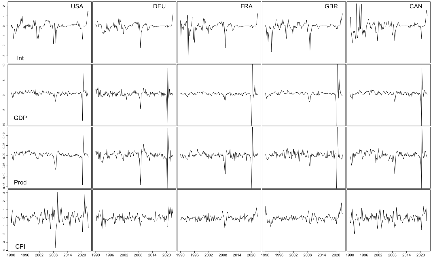
Figure 1: Time series of four economic indicators from five countries.

2 Model Formulation

2.1 The MAR Model

Let $\bm{Y}_{t}\in\mathbb{R}^{m\times n},~{}1\leq t\leq T$ be the matrix-valued time series data. The $p$th-order matrix autoregressive model, denoted by MAR($p$), specifies the relationship,

$$\bm{Y}_{t}=\bm{C}+\sum_{i=1}^{p}\bm{A}_{i}\bm{Y}_{t-i}\bm{B}_{i}^{\mathsf{T}}+\bm{E}_{t},$$ (1)

where $\bm{A}_{i}\in\mathbb{R}^{m\times m}$ and $\bm{B}_{i}\in\mathbb{R}^{n\times n}$ are parameter matrices, and $\bm{E}_{t}$ is the matrix of random errors. The parameter matrix $\bm{C}$ is the intercept matrix, which is generally absent for centered data. This model admits some interesting interpretations. For example, in an MAR(1) model, the parameter matrices $\bm{A}_{1}$ and $\bm{B}_{1}^{\mathsf{T}}$ reflects row-wise and column-wise interactions, respectively; it can also be viewed as factor regression model, with the factor being $\bm{Y}_{t-1}\bm{B}_{1}^{\mathsf{T}}$ (Chen et al.,, 2021).

Let $\mathrm{vec}{\left(\cdot\right)}$ denote the vectorization of the enclosed matrix via stacking its columns. Also, let the operator $\mathrm{vech}{\left(\cdot\right)}$ denote the half-vectorization of a symmetric matrix. The MAR($p$) model can be expressed as

$$\mathrm{vec}{\left(\bm{Y}_{t}\right)}=\mathrm{vec}{\left(\bm{C}\right)}+\sum_{i=1}^{p}\left(\bm{B}_{i}\otimes\bm{A}_{i}\right)\mathrm{vec}{\left(\bm{Y}_{t-i}\right)}+\mathrm{vec}{\left(\bm{E}_{t}\right)},$$ (2)

where $\otimes$ represents the Kronecker product of matrices. Hence the MAR($p$) model is intrinsically a constrained $p$th-order VAR model. It is assumed that $\{\bm{E}_{t}~{}|~{}1\leq t\leq T\}$ is a sequence of independent and identically distributed (i.i.d.) random matrices such that $\bm{E}_{t}$ is independent of $\{\bm{Y}_{t-1},\bm{Y}_{t-2},\dots\}$. Also, $\mathbb{E}{\left(\bm{E}_{t}\right)}=\bm{0}$ and ${\rm Var}\left(\mathrm{vec}{\left(\bm{E}_{t}\right)}\right)=\bm{\Sigma}$, where $\bm{\Sigma}$ is positive definite. Throughout, we denote $\bm{0}$ as either a zero matrix or a zero vector with a suitable dimension.

We can further specify that $\bm{\Sigma}$ is separable: $\bm{\Sigma}=\bm{V}\otimes\bm{U}$, where $\bm{U}\in\mathrm{R}^{m\times m}$ and $\bm{V}\in\mathbb{R}^{n\times n}$ are all positive definite matrices. This covariance structure has gained significant attention in multivariate analysis, especially in cases where variables can be cross-classified by two factors, such as spatiotemporal data. Hypothesis tests have also been developed for this separable covariance structure, see, e.g., Lu and Zimmerman, (2005). Let $\mathscr{F}_{t}$ be the $\sigma$-algebra generated by $\bm{Y}_{t-j}$, $j\geq 0$. Under the separability assumption of $\bm{\Sigma}$, if $\{\bm{E}_{t}~{}|~{}1\leq t\leq T\}$ is normally distributed, then the conditional distribution of $\bm{Y}_{t}$ given $\mathscr{F}_{t-1}$ follows a matrix normal distribution with mean $\bm{C}+\sum_{i=1}^{p}\bm{A}_{i}\bm{Y}_{t-i}\bm{B}_{i}^{\mathsf{T}}$ and variance-covariance matrices $\bm{U}$ and $\bm{V}$, in symbol, $\bm{Y}_{t}\sim\mathcal{MN}_{m,n}(\bm{C}+\sum_{i=1}^{p}\bm{A}_{i}\bm{Y}_{t-i}\bm{B}_{i}^{\mathsf{T}},\bm{U},\bm{V})$, whose joint probability density function is given by,

$$f_{\mathcal{MN}}(\bm{Y}_{t}|\bm{C}+\sum_{i=1}^{p}\bm{A}_{i}\bm{Y}_{t-i}\bm{B}_{i}^{\mathsf{T}},\bm{U},\bm{V})=\frac{\exp\left(-\frac{1}{2}\mathrm{tr}{\left[\bm{V}^{-1}\bm{\epsilon}_{t}^{\mathsf{T}}\bm{U}^{-1}\bm{\epsilon}_{t}\right]}\right)}{(2\pi)^{mn/2}\det(\bm{V})^{m/2}\det(\bm{U})^{n/2}},$$ (3)

where $\bm{\epsilon}_{t}=\bm{Y}_{t}-\bm{C}-\sum_{i=1}^{p}\bm{A}_{i}\bm{Y}_{t-i}\bm{B}_{i}^{\mathsf{T}}$, and $\det(\cdot)$ denotes the determinant of the enclosed matrix. It can be shown that, if $\bm{Y}_{t}\sim\mathcal{MN}_{m,n}(\bm{C}+\sum_{i=1}^{p}\bm{A}_{i}\bm{Y}_{t-i}\bm{B}_{i}^{\mathsf{T}},\bm{U},\bm{V})$, then $\mathrm{vec}{\left(\bm{Y}_{t}\right)}$ follows an $mn$-dimensional multivariate normal distribution with mean $\mathrm{vec}{\left(\bm{C}+\sum_{i=1}^{p}\bm{A}_{i}\bm{Y}_{t-i}\bm{B}_{i}^{\mathsf{T}}\right)}$ and variance-covariance matrix $\bm{V}\otimes\bm{U}$, denoted as $\mathrm{vec}{\left(\bm{Y}_{t}\right)}\sim\mathcal{N}_{mn}(\mathrm{vec}{\left(\bm{C}+\sum_{i=1}^{p}\bm{A}_{i}\bm{Y}_{t-i}\bm{B}_{i}^{\mathsf{T}}\right)},\bm{V}\otimes\bm{U})$, whose joint probability density function is $f_{\mathcal{N}}(\mathrm{vec}{\left(\bm{Y}_{t}\right)}|\mathrm{vec}{\left(\bm{C}+\sum_{i=1}^{p}\bm{A}_{i}\bm{Y}_{t-i}\bm{B}_{i}^{\mathsf{T}}\right)},\bm{V}\otimes\bm{U}).$

Notice that, the MAR($p$) model is not identifiable as the model is unchanged by multiplying $\bm{A}_{i}$ by some non-zero constant and dividing $\bm{B}_{i}$ by the same constant, for any $i\in\{1,\dots,p\}$, and so do $\bm{U}$ and $\bm{V}$. Thus, the model requires some identifiability constraints, for example, $\|\bm{B}_{i}\|_{F}=\|\bm{V}\|_{F}=1$, and the first non-zero element of $\mathrm{vec}{\left(\bm{B}_{i}\right)}$ is positive for $1\leq i\leq p$, where $\|\cdot\|_{F}$ denotes the Frobenius norm of the enclosed matrix.

2.2 The MMAR Model

The MMAR($K;p_{1},\dots,p_{K})$ model consists of a probabilistic mixture of $K$ normal MAR sub-processes, which specifies that the conditional density of $\bm{Y}_{t}|\mathscr{F}_{t-1}$ is equal to,

$$\sum_{k=1}^{K}\alpha_{k}f_{\mathcal{MN}}\left(\bm{Y}_{t}|\bm{C}_{k}+\sum_{i=1}^{p_{k}}\bm{A}_{k,i}\bm{Y}_{t-i}\bm{B}_{k,i}^{\mathsf{T}},\bm{U}_{k},\bm{V}_{k}\right),$$ (4)

where $p_{k}$ is the autoregressive order of the $k$th component, $0<\alpha_{k}<1$ is the mixing weight of the $k$th component such that $\sum_{k=1}^{K}\alpha_{k}=1$, $\bm{C}_{k}\in\mathbb{R}^{m\times n}$ is the intercept matrix, $\bm{A}_{k,i}\in\mathbb{R}^{m\times m}$ and $\bm{B}_{k,i}\in\mathbb{R}^{n\times n}$ are the non-zero coefficient matrices of the $k$th component, and $\bm{U}_{k}\in\mathbb{R}^{m\times m}$ and $\bm{V}_{k}\in\mathbb{R}^{n\times n}$ are the corresponding positive definite variance-covariance matrices. The conditional density (4) is equal to,

$$\sum_{k=1}^{K}\alpha_{k}\left\{\frac{\exp\left(-\frac{1}{2}\mathrm{tr}{\left[\bm{V}_{k}^{-1}\bm{\epsilon}_{t,k}^{\mathsf{T}}\bm{U}_{k}^{-1}\bm{\epsilon}_{t,k}\right]}\right)}{(2\pi)^{mn/2}\det(\bm{V}_{k})^{m/2}\det(\bm{U}_{k})^{n/2}}\right\},$$

where

$$\bm{\epsilon}_{t,k}=\bm{Y}_{t}-\bm{C}_{k}-\sum_{i=1}^{p_{k}}\bm{A}_{k,i}\bm{Y}_{t-i}\bm{B}_{k,i}^{\mathsf{T}}.$$ (5)

Since each MAR component in the mixture has a vector representation in the form of $\eqref{MAR_V}$, the mixture density (4) has the following representation:

$$\sum_{k=1}^{K}\alpha_{k}f_{\mathcal{N}}\left(\mathrm{vec}{\left(\bm{Y}_{t}\right)}|\mathrm{vec}{\left(\bm{C}_{k}\right)}+\sum_{i=1}^{p_{k}}(\bm{B}_{k,i}\otimes\bm{A}_{k,i})\mathrm{vec}{\left(\bm{Y}_{t-i}\right)},\bm{V}_{k}\otimes\bm{U}_{k}\right).$$ (6)

In comparison, the mixture VAR model introduced by Fong et al., (2007) specifies the conditional density as,

$$\sum_{k=1}^{K}\alpha_{k}f_{\mathcal{N}}\left(\mathrm{vec}{\left(\bm{Y}_{t}\right)}|\bm{\Psi}_{k,0}+\sum_{i=1}^{p_{k}}\bm{\Psi}_{k,i}\mathrm{vec}{\left(\bm{Y}_{t-i}\right)},\bm{\Omega}_{k}\right),$$ (7)

where for each $k\in\{1,\dots,K\}$, $\bm{\Psi}_{k,0}$ is an $mn$-dimensional vector, $\bm{\Psi}_{k,i}\in\mathbb{R}^{mn\times mn}$ is a coefficient matrix for $1\leq i\leq p_{k}$, and $\bm{\Omega}_{k}\in\mathbb{R}^{mn\times mn}$ is a variance-covariance matrix. Hence, the proposed MMAR model can be viewed as a constrained version of the mixture VAR model with the restrictions,

$$\bm{\Psi}_{k,0}=\mathrm{vec}{\left(\bm{C}_{k}\right)},~{}~{}\bm{\Psi}_{k,i}=\bm{B}_{k,i}\otimes\bm{A}_{k,i},~{}~{}\bm{\Omega}_{k}=\bm{V}_{k}\otimes\bm{U}_{k}.$$

For each $k$ and $i$, the parameter matrix $\bm{\Psi}_{k,i}$ in the unconstrained mixture VAR model contains $m^{2}n^{2}$ parameters, while its counterpart in the MMAR model $\bm{A}_{k,i}$ and $\bm{B}_{k,i}$ only require $m^{2}+n^{2}$ parameters in total. Similarly, $\bm{\Omega}_{k}$ contains $m^{2}n^{2}$ parameters while $\bm{U}_{k}$ and $\bm{V}_{k}$ only require $m^{2}+n^{2}$ parameters. It is evident that the number of unknown parameters in the mixture VAR model could be significantly greater than that of the MMAR model, particularly when the matrix observations are of large dimensions and the model consists of many mixture components with high AR orders. Therefore, comparing with the mixture VAR model, the proposed MMAR model not only preserves the matrix structure, but also results in a substantial reduction in dimensionality.

Similar to the mixture VAR model, the MMAR model has the following interesting properties. First, it can contain both stationary and non-stationary MAR components while maintaining overall model stationarity. An intuitive way to understand this is that the stationary components exhibit contraction patterns, whereas non-stationary components display expansion patterns. The overall model achieves stationarity when the contraction patterns dominate over the expansion patterns. Second, it has the capability to model the multi-modality of matrix-valued time series, which properties we will illustrate through examples.

The MMAR($K;p_{1},\dots,p_{K}$) model has similar identifiability issues as the MAR model, as for each $k\in\{1,\dots,K\}$ and $i\in\{1,\dots,p_{k}\}$, $\bm{A}_{k,i}$ and $\bm{B}_{k,i}$ are identifiable up to a constant, and so are $\bm{U}_{k}$ and $\bm{V}_{k}$. Therefore, the following constraints are imposed: the first non-zero element of $\mathrm{vec}{\left(\bm{B}_{k,i}\right)}$ is positive, and

$$\|\bm{B}_{k,i}\|_{F}=1,~{}~{}~{}k\in\{1,2,\dots,K\},~{}i\in\{1,\dots,p_{k}\},$$ (8)

$$\|\mathrm{vech}{\left(\bm{V}_{k}^{-1}\right)}\|_{F}=1,~{}~{}~{}k\in\{1,2,\dots,K\}.$$ (9)

Without loss of generality, we assume that the first element of $\mathrm{vec}{\left(\bm{B}_{k,i}\right)}$ is positive. In addition, to circumvent the label-switching problem for the mixture models (McLachlan and Peel,, 2000), the following constraints are required:

$$0<\alpha_{1}<\alpha_{2}<\cdots<\alpha_{K}<1,$$ (10)

$$f_{\mathcal{N}}\left(\mathrm{vec}{\left(\bm{Y}_{t}\right)}|\mathrm{vec}{\left(\bm{C}_{k}\right)}+\sum_{i=1}^{p_{k}}(\bm{B}_{k,i}\otimes\bm{A}_{k,i})\mathrm{vec}{\left(\bm{Y}_{t-i}\right)},\bm{V}_{k}\otimes\bm{U}_{k}\right)$$

$$\neq f_{\mathcal{N}}\left(\mathrm{vec}{\left(\bm{Y}_{t}\right)}|\mathrm{vec}{\left(\bm{C}_{j}\right)}+\sum_{i=1}^{p_{j}}(\bm{B}_{j,i}\otimes\bm{A}_{j,i})\mathrm{vec}{\left(\bm{Y}_{t-i}\right)},\bm{V}_{j}\otimes\bm{U}_{j}\right),~{}~{}\forall k\neq j.$$ (11)

3 Stationarity

To study the strict and weak stationarity conditions for the proposed MMAR model, we use the fact that a mixture autoregressive model can be embedded in a stochastic difference equation (SDE) model, which is also known as the random coefficient autoregression (Douc et al.,, 2014). Let $p_{\max}=\max\{p_{1},\dots,p_{K}\}$. For $p_{k}\neq p_{\max}$, define

$$\bm{A}_{k,i}=\bm{0},\quad\bm{B}_{k,i}=\bm{0},\quad p_{k}<i\leq p_{\max}.$$

Let $\bm{y}_{t}=\mathrm{vec}{\left(\bm{Y}_{t}\right)}$, $t\in\{1,\dots,T\}$, and

$$\mathcal{X}_{t}=\begin{pmatrix}\bm{y}_{t}\\ \bm{y}_{t-1}\\ \vdots\\ \bm{y}_{t-p_{\max}+1}\end{pmatrix},$$ (12)

$$\bm{\Phi}_{k}=\begin{pmatrix}\bm{B}_{k,1}\otimes\bm{A}_{k,1}&\bm{B}_{k,2}\otimes\bm{A}_{k,2}&\dots&\bm{B}_{k,p_{\max}-1}\otimes\bm{A}_{k,p_{\max}-1}&\bm{B}_{k,p_{\max}}\otimes\bm{A}_{k,p_{\max}}\\ \bm{I}_{mn}&\bm{0}&\dots&\bm{0}&\bm{0}\\ \bm{0}&\bm{I}_{mn}&\dots&\bm{0}&\bm{0}\\ \vdots&\vdots&\ddots&\vdots&\vdots\\ \bm{0}&\bm{0}&\dots&\bm{I}_{mn}&\bm{0}\end{pmatrix},$$

$$\mathcal{C}_{k}=\begin{pmatrix}\bm{C}_{k}\\ \bm{0}\\ \vdots\\ \bm{0}\end{pmatrix},\qquad\mathcal{E}_{t,k}=\begin{pmatrix}\bm{E}_{t,k}\\ \bm{0}\\ \vdots\\ \bm{0}\end{pmatrix},$$

where $\bm{I}_{mn}$ is the $mn\times mn$ identity matrix, and $\{\bm{E}_{t,k}\}$ is a sequence of i.i.d. random normal matrices with $\bm{0}$ and variance-covariance matrices $\bm{U}_{k}$ and $\bm{V}_{k}$. Also, $\bm{E}_{t,k}$ is independent of $\{\bm{Y}_{t-1},\bm{Y}_{t-2},\dots\}$. Then the MMAR$(K;p_{1},\dots,p_{K})$ has the following representation as a first-order mixture VAR model:

$$\mathcal{X}_{t}=\mathcal{C}_{k}+\bm{\Phi}_{k}\mathcal{X}_{t-1}+\mathcal{E}_{t,k},\quad\mathrm{with~{}probability}~{}\alpha_{k},~{}1\leq k\leq K.$$

Let $\{(\bm{D}_{t},\bm{\eta}_{t})\}$ be a sequence of strictly stationary and ergodic random elements. The SDE model for $\mathcal{X}_{t}$ is defined as,

$$\mathcal{X}_{t}=\bm{D}_{t}\mathcal{X}_{t-1}+\bm{\eta}_{t},$$ (13)

If $\{(\bm{D}_{t},\bm{\eta}_{t})\}$ is set to be a sequences of i.i.d. random elements such that,

$$\Pr(\bm{D}_{t}=\bm{\Phi}_{k}~{}~{}\text{and}~{}~{}\bm{\eta}_{t}=\mathcal{C}_{k}+\mathcal{E}_{t,k})=\alpha_{k},~{}~{}~{}~{}1\leq k\leq K,$$ (14)

then the MMAR($K,p_{1},\dots,p_{K}$) model (4) coincides with the SDE model (13). Let $\|\cdot\|$ denote an arbitrary but fixed matrix norm. For the SDE model (13), if $\mathbb{E}{\left(\log^{+}(\|\bm{D}_{1}\|)\right)}<\infty$, then its top-Lyapunov exponent is defined as

$$\gamma=\lim_{t\to\infty}\frac{1}{t}\mathbb{E}{\left(\log\|\bm{D}_{t}\bm{D}_{t-1}\dots\bm{D}_{1}\|\right)}=\inf_{t\in\mathbb{N}^{*}}\frac{1}{t}\mathbb{E}{\left(\log\|\bm{D}_{t}\bm{D}_{t-1}\dots\bm{D}_{1}\|\right)}.$$ (15)

Assume that $\{(\bm{D}_{t},\bm{\eta}_{t})\}$ is i.i.d., then the $q$th norm Lyapunov coefficient is defined as,

$$\gamma_{q}=\lim_{t\to\infty}\frac{1}{t}\log\left(\mathbb{E}^{1/q}\left(\|\bm{D}_{t}\bm{D}_{t-1}\dots\bm{D}_{1}\|^{q}\right)\right)=\inf_{t\in\mathbb{N}^{*}}\frac{1}{t}\log\left(\mathbb{E}^{1/q}\left(\|\bm{D}_{t}\bm{D}_{t-1}\dots\bm{D}_{1}\|^{q}\right)\right),$$ (16)

where $q>0$. Neither $\gamma$ nor $\gamma_{q}$ depends on the choice of the matrix norm $\|\cdot\|$ (Douc et al.,, 2014).

3.1 Strict Stationarity

The strict stationarity of the MMAR model is established by the following proposition.

Proposition 1.

Assume that $\{(\bm{D}_{t},\bm{\eta}_{t})\}$ is a sequence of i.i.d. random elements such that (14) holds. If the top-Lyapunov exponent, defined by (15), is strictly negative. Then the MMAR model has a unique strictly stationary solution given by,

$$\tilde{\mathcal{X}_{t}}=\sum_{j=0}^{\infty}\left(\prod_{i=t-j+1}^{t}\bm{D}_{i}\right)\bm{\eta}_{t-j}.$$ (17)

A sufficient condition for the top-Lyapunov exponent $\gamma$ to be strictly negative is that,

$$\mathbb{E}{\left(\log\|\bm{D}_{1}\|\right)}=\sum_{k=1}^{K}\alpha_{k}\log(\|\bm{\Phi}_{k}\|)<0.$$

Let $\rho(\bm{\Phi}_{k})$ denotes the spectral radius of $\bm{\Phi}_{k}$. By the relationship between the spectral radius and matrix norms, for any $\varepsilon>0$, there exists a matrix norm $\|\cdot\|_{*}$, such that,

$$\rho(\bm{\Phi}_{k})\leq\|\bm{\Phi}_{k}\|_{*}\leq\rho(\bm{\Phi}_{k})+\varepsilon.$$ (18)

By the arbitrariness of $\varepsilon$, we derive the following corollary:

Corollary 1.

A sufficient condition for the MMAR($K;p_{1},\dots,p_{K}$) model to have a strictly stationary and ergodic solution is $\sum_{k=1}^{K}\alpha_{k}\log(\rho(\bm{\Phi}_{k}))<0$. For an MMAR($K;1,\dots,1$) model, the condition can be simplified to,

$$\sum_{k=1}^{K}\alpha_{k}\log(\rho(\bm{B}_{k,1})\rho(\bm{A}_{k,1}))<0.$$

Remark. If $\rho(\bm{\Phi}_{k})<1$, then the $k$th component MAR process is stationary. Therefore, by Corollary (1) if all the component are stationary, then the MMAR model is also stationary.

The ergodicity of the MMAR model is established by the following proposition.

Proposition 2.

Let $\{\bm{Y}_{t}\}$ be an MMAR process, and $\mathcal{X}_{t}$ defined in (12). If $\{\mathcal{X}_{t}\}$ is strictly stationary, and the initial values are generated from the stationary distribution, then it is also ergodic.

3.2 Weak Stationarity

The tails of the stationary solutions are heavier than those of $\bm{\eta}_{t}$, and may not have finite second-order moments even if $\bm{\eta}_{t}$ is Gaussian (Douc et al.,, 2014, pp. 91–92). Thus, it is possible that the MMAR model is strictly stationary but not second-order (weakly) stationary. For the MMAR($K;1,\dots,1$) model, its first-order and the second-order stationarity conditions can be established based on the results in Fong et al., (2007).

Proposition 3.

The MMAR($K;1,\dots,1$) model is stationary in the mean if and only if all the eigenvalues of $\sum_{k=1}^{K}\alpha_{k}(\bm{B}_{k,1}\otimes\bm{A}_{k,1})$ have modulus less than 1.

Proposition 4.

Assume the MMAR($K;1,\dots,1$) model is stationary in the mean. Then it is second-order stationary if and only if all the eigenvalues of $\sum_{k=1}^{K}\alpha_{k}\{(\bm{B}_{k,1}\otimes\bm{A}_{k,1})\otimes(\bm{B}_{k,1}\otimes\bm{A}_{k,1})\}$ have modulus less than 1.

Next, we consider the conditions for the existence of $q$th-order stationary solutions to the MMAR ($K;p_{1},\dots,p_{K}$) model. The following proposition gives the conditions for the stationary solutions of the MMAR model to admit moments of order $q\geq 1$.

Proposition 5.

Assume that $\{(\bm{D}_{t},\bm{\eta}_{t})\}$ is a sequence of i.i.d. random elements such that (14) holds. If the $q$th norm Lyapunov coefficient, defined by (16), is strictly negative. Then the MMAR model has a unique strictly stationary solution, whose vectorization is given in (17), such that $\mathbb{E}{\left(\|\tilde{\mathcal{X}_{t}}\|^{q}\right)}<\infty$. Moreover, the right-hand-side of (17) converges in the $q$th norm.

Similar to the top-Lyapunov coefficient $\gamma$, a sufficient condition for $\gamma_{q}<0$ is $\log\left(\mathbb{E}^{1/q}(\|\bm{D}_{1}\|^{q})\right)<0,$ which is equivalent to

$$\mathbb{E}(\|\bm{D}_{1}\|^{q})=\sum_{k=1}^{K}\alpha_{k}\|\bm{\Phi}_{k}\|^{q}<1.$$

Using (18) once again, we can derive the following corollary.

Corollary 2.

A sufficient condition for the MMAR($K;p_{1},\dots,p_{K}$) model to have a stationary and ergodic solution with finite $q$th moment is $\sum_{k=1}^{K}(\rho(\bm{\Phi}_{k}))^{q}<1.$ For the MMAR($K;1,\dots,1$) model, the condition can be expressed as,

$$\sum_{k=1}^{K}\alpha_{k}(\rho(\bm{B}_{k,1})\rho(\bm{A}_{k,1}))^{q}<1.$$

Below, we exhibit an MMAR model comprising both stationary and nonstationary components, while the overall model is strictly stationary.
Example 1: Consider an MMAR($2;1,1$) model. Let $\bm{Y}_{t}\in\mathbb{R}^{2\times 2}$, $\alpha_{1}=0.4$, $\alpha_{2}=0.6$, and

$$\bm{B}_{1,1}\otimes\bm{A}_{1,1}=\begin{pmatrix}0.3&0.4\\ 0.6&0.3\end{pmatrix}\otimes\begin{pmatrix}0.5&0.7\\ 0.55&0.4\end{pmatrix},$$

$$\bm{B}_{2,1}\otimes\bm{A}_{2,1}=\begin{pmatrix}0.6&0.3\\ 0.2&0.4\end{pmatrix}\otimes\begin{pmatrix}1.1&0.2\\ 0.4&1.2\end{pmatrix},$$

Also, we assume that $\bm{C}_{1}=\bm{C}_{2}=\bm{0}$ and $\bm{V}_{1}\otimes\bm{U}_{1}=\bm{V}_{2}\otimes\bm{U}_{2}=\bm{I}_{4}$. By Proposition 1 in Chen et al., (2021), the first MAR component is second-order stationary as $\rho(\bm{B}_{1,1}\otimes\bm{A}_{1,1})=0.8471<1$, while the second MAR component is not because $\rho(\bm{B}_{2,1}\otimes\bm{A}_{2,1})=1.0989>1$. But the overall model is strictly stationary as $\sum_{k=1}^{2}\alpha_{k}\log(\rho(\bm{B}_{k}\otimes\bm{A}_{k}))=-0.0018<0$. But it is neither first-order nor second-order stationary, as the spectral radii of $\sum_{k=1}^{2}\alpha_{k}(\bm{B}_{k}\otimes\bm{A}_{k})$ and $\sum_{k=1}^{2}\alpha_{k}\{(\bm{B}_{k}\otimes\bm{A}_{k})\otimes(\bm{B}_{k}\otimes\bm{A}_{k})\}$ are all larger than 1. Figure 2 shows a simulated dataset of size 1200 of Example 1.

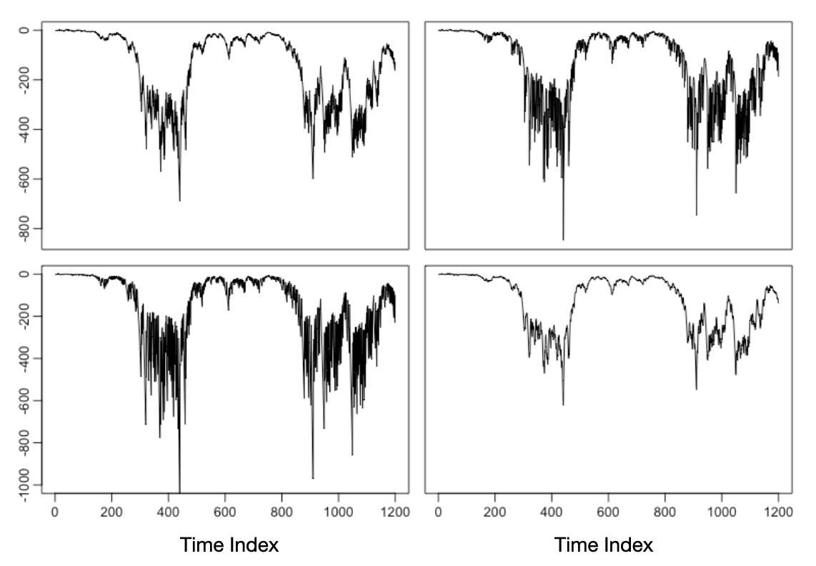
Figure 2: Simulated data of Example 1.

We would like to mention that the overall model can be made overall second-order stationary by making minor adjustments to the example’s parameters, while preserving the non-stationarity of the second component process.

4 Parameter Estimation

Maximum likelihood estimation of the MMAR model can be implemented via an Expectation–Maximization (EM) algorithm (Dempster et al.,, 1977). Let $\bm{Z}_{t}=(Z_{t,1},\dots,Z_{t,K})$ be the latent variable, such that $Z_{t,k}=1$ if $\bm{Y}_{t}$ is from the $k$th component, and equals 0 otherwise. For simplicity, define

$$\mathcal{A}_{k}=\begin{pmatrix}\bm{A}_{k,1},\dots,\bm{A}_{k,p_{k}}\end{pmatrix},\quad\mathcal{B}_{k}=\begin{pmatrix}\bm{B}_{k,1},\dots,\bm{B}_{k,p_{k}}\end{pmatrix},$$

and $\mathcal{Z}_{t-1,k}=\mathrm{Bdiag}(\bm{Y}_{t-1},\dots,\bm{Y}_{t-p_{k}})$, a $pm\times pn$ block-diagonal matrix, with $\{\bm{Y}_{t-1},\dots,\bm{Y}_{t-p_{k}}\}$ comprising the diagonal blocks. The density of $(\bm{Y}_{t},\bm{Z}_{t})$ given $\mathscr{F}_{t-1}$ is

$$\prod_{k=1}^{K}\alpha_{k}^{Z_{t,k}}\left\{\frac{\exp\left(-\frac{1}{2}\mathrm{tr}{\left[\bm{V}_{k}^{-1}\bm{\epsilon}_{t,k}^{\mathsf{T}}\bm{U}_{k}^{-1}\bm{\epsilon}_{t,k}\right]}\right)}{(2\pi)^{mn/2}\det(\bm{V}_{k})^{m/2}\det(\bm{U}_{k})^{n/2}}\right\}^{Z_{t,k}}.$$

E-step: Let $\tau_{t,k}$ be the conditional expectation of the $Z_{t,k}$ given $\mathscr{F}_{t}$ and the current parameter value. Then

$$\tau_{t,k}=\frac{\alpha_{k}\det(\bm{V}_{k})^{-m/2}\det(\bm{U}_{k})^{-n/2}\exp\left(-\frac{1}{2}\mathrm{tr}{\left[\bm{V}_{k}^{-1}\bm{\epsilon}_{t,k}^{\mathsf{T}}\bm{U}_{k}^{-1}\bm{\epsilon}_{t,k}\right]}\right)}{\sum_{j=1}^{K}\alpha_{j}\det(\bm{V}_{j})^{-m/2}\det(\bm{U}_{j})^{-n/2}\exp\left(-\frac{1}{2}\mathrm{tr}{\left[\bm{V}_{j}^{-1}\bm{\epsilon}_{t,k}^{\mathsf{T}}\bm{U}_{j}^{-1}\bm{\epsilon}_{t,k}\right]}\right)}.$$

M-step: Update the estimates of $\alpha$’s as follows:

$$\hat{\alpha}_{k}=\frac{1}{T-p_{\max}}\sum_{t=p_{\max}+1}^{T}\tau_{t,k}.$$

The estimates of $\mathcal{A}_{k}$, $\mathcal{B}_{k}$, $\bm{C}_{k}$, $\bm{U}_{k}$ and $\bm{V}_{k}$ must satisfy the following gradient conditions:

$$\mathcal{A}_{k}=\left(\sum_{t=p_{\max}+1}^{T}\tau_{t,k}(\bm{Y}_{t}-\bm{C}_{k})\bm{V}_{k}^{-1}\mathcal{B}_{k}\mathcal{Z}_{t-1,k}^{\mathsf{T}}\right)\left(\sum_{t=p_{\max}+1}^{T}\tau_{t,k}\mathcal{Z}_{t-1,k}\mathcal{B}_{k}^{\mathsf{T}}\bm{V}_{k}^{-1}\mathcal{B}_{k}\mathcal{Z}_{t-1,k}^{\mathsf{T}}\right)^{-1},$$ (19)

$$\mathcal{B}_{k}=\left(\sum_{t=p_{\max}+1}^{T}\tau_{t,k}(\bm{Y}_{t}-\bm{C}_{k})^{\mathsf{T}}\bm{U}_{k}^{-1}\mathcal{A}_{k}\mathcal{Z}_{t-1,k}\right)\left(\sum_{t=p_{\max}+1}^{T}\tau_{t,k}\mathcal{Z}_{t-1,k}^{\mathsf{T}}\mathcal{A}_{k}^{\mathsf{T}}\bm{U}_{k}^{-1}\mathcal{A}_{k}\mathcal{Z}_{t-1,k}\right)^{-1},$$ (20)

$$\bm{C}_{k}=\frac{\sum_{t=p_{\max}+1}^{T}\tau_{t,k}(\bm{Y}_{t}-\mathcal{A}_{k}\mathcal{Z}_{t-1,k}\mathcal{B}_{k}^{\mathsf{T}})}{\sum_{t=p_{\max}+1}^{T}\tau_{t,k}},$$ (21)

$$\bm{U}_{k}=\frac{\sum_{t=p_{\max}+1}^{T}\tau_{t,k}(\bm{Y}_{t}-\bm{C}_{k}-\mathcal{A}_{k}\mathcal{Z}_{t-1,k}\mathcal{B}_{k}^{\mathsf{T}})\bm{V}_{k}^{-1}(\bm{Y}_{t}-\bm{C}_{k}-\mathcal{A}_{k}\mathcal{Z}_{t-1,k}\mathcal{B}_{k}^{\mathsf{T}})^{\mathsf{T}}}{n\sum_{t=p_{\max}+1}^{T}\tau_{t,k}},$$ (22)

$$\bm{V}_{k}=\frac{\sum_{t=p_{\max}+1}^{T}\tau_{t,k}(\bm{Y}_{t}-\bm{C}_{k}-\mathcal{A}_{k}\mathcal{Z}_{t-1,k}\mathcal{B}_{k}^{\mathsf{T}})^{\mathsf{T}}\bm{U}_{k}^{-1}(\bm{Y}_{t}-\bm{C}_{k}-\mathcal{A}_{k}\mathcal{Z}_{t-1,k}\mathcal{B}_{k}^{\mathsf{T}})}{m\sum_{t=p_{\max}+1}^{T}\tau_{t,k}}.$$ (23)

Closed-form solutions for these parameter estimates do not exist. However, the optimization problem in each M-step can be solved by a blockwise coordinate descent algorithm. To be specific, we use equations (19) – (23) to iteratively update one of $\{\mathcal{A}_{k},\mathcal{B}_{k},\bm{C}_{k},\bm{U}_{k},\bm{V}_{k}\}$ with all of the others being fixed. Note that the target function in each of the M-steps is multimodal, and the blockwise coordinate descent algorithm may converge to a local maximum.

The EM algorithm is known to converge to a local maximum. Nevertheless, given the intricate structure of the target function, numerous local maxima can exist, particularly in high-dimensional scenarios, making it necessary to repeat the process many times. The speed of the proposed EM algorithm could be very slow, as it involves an iterative process to find the maximum within each of the M-step.

We propose an initial value selection method based on the pattern in the longitudinal relational data observed by Hoff, (2015), where two scalar time series can be positively correlated even if they are in different rows and columns. This pattern is not limited to longitudinal relational data but is also observed in other matrix-valued time series datasets, such as the economic indicators dataset displayed in Figure 1 and the simulated dataset shown in Figure 2. Further investigation in the simulations reveals that the correlations could also be negative. Therefore, an univariate time series can provide insights into the clustering patterns of the entire dataset. Based on this, we suggest the following procedure. First, select an arbitrary scalar time series from the matrix-valued time series data, and fit a scalar mixture autoregressive with $K$ components. Second, divide the whole process into $K$ parts based on the fitted scalar model. Third, within each part, fit a matrix autoregressive model via maximum likelihood, and use the estimate so obtained as the initial value for one component of the MMAR model. This procedure can be repeated multiple times to implement the EM algorithm with different sets of initial values.

5 Asymptotics

The parameter for the $k$th component is,

$$\bm{\theta}_{k}= \big{(}\mathrm{vec}{\left(\bm{A}_{k,1}\right)}^{\mathsf{T}},\mathrm{vec}_{-1}{\left(\bm{B}_{k,1}\right)}^{\mathsf{T}},\dots,\mathrm{vec}{\left(\bm{A}_{k,p_{k}}\right)}^{\mathsf{T}},$$

$$\mathrm{vec}_{-1}{\left(\bm{B}_{k,p_{k}}\right)}^{\mathsf{T}},\mathrm{vec}{\left(\bm{C}_{k}\right)}^{\mathsf{T}},\mathrm{vech}{\left(\bm{U}_{k}^{-1}\right)}^{\mathsf{T}},\mathrm{vech}_{-1}{\left(\bm{V}_{k}^{-1}\right)}^{\mathsf{T}}\big{)}^{\mathsf{T}},$$

where the operator $\mathrm{vec}_{-1}{\left(\cdot\right)}$ means vectorizing the enclosed matrix with its first element removed, and $\mathrm{vech}_{-1}{\left(\cdot\right)}$ is similarly defined. Those elements are removed due to identifiability constraints (8) and (9). It is easily seen that the model identifiability constraint (2.2) is equivalent to,

$$\bm{\theta}_{k}\neq\bm{\theta}_{j},\qquad\forall k,j\in\{1,2,\dots,K\},~{}~{}k\neq j.$$ (24)

Therefore, the parameter of interest for the MMAR($K;p_{1},\dots,p_{K}$) model is

$$\bm{\theta}=(\bm{\theta}_{1},\dots,\bm{\theta}_{K},\alpha_{1},\dots,\alpha_{K-1}),$$

where $\alpha_{K}$ is excluded as $\alpha_{K}=1-\sum_{k=1}^{K-1}\alpha_{k}$. To simplify the notations, define,

$$f_{t}(\bm{y}_{t}|\mathscr{F}_{t-1};\bm{\theta}_{k})=\det(2\pi\bm{V}_{k}\otimes\bm{U}_{k})^{-1/2}\exp\left\{-\frac{1}{2}\mathrm{vec}{\left(\bm{\epsilon}_{t,k}\right)}^{\mathsf{T}}(\bm{V}_{k}\otimes\bm{U}_{k})^{-1}\bm{\epsilon}_{t,k}\right\}.$$ (25)

Condition on $\mathscr{F}_{p_{\max}}$, the log-likelihood function is $L_{T}(\bm{\theta})=\sum_{t=p_{\max}+1}^{T}l_{t}(\bm{\theta})$, where $l_{t}(\bm{\theta})=\log\left(\sum_{k=1}^{K}\alpha_{k}f_{t}(\bm{y}_{t}|\mathscr{F}_{t-1};\bm{\theta}_{k})\right).$ Also, denote $\dot{l}_{t}(\bm{\theta})=\frac{\partial{l}_{t}(\bm{\theta})}{\partial\bm{\theta}}$ and $\ddot{l}_{t}(\bm{\theta})=\frac{\partial^{2}{l}_{t}(\bm{\theta})}{\partial\bm{\theta}\partial\bm{\theta}^{\mathsf{T}}}$ the first and second derivatives of $l_{t}(\bm{\theta})$, respectively. Let $\bm{\theta}^{0}$ be the true parameter, and $\Theta$ be the parameter space. The dimensionality of $\Theta$ is

$$\mathrm{dim}(\Theta)=K-1+Kmn+\sum_{k=1}^{K}\left(p_{k}(m^{2}+n^{2}-1)+m(m+1)/2+n(n+1)/2-1\right).$$

Denote $\hat{\bm{\theta}}=\operatorname*{arg\,max}_{\bm{\theta}\in\Theta}L_{T}(\bm{\theta})$ the MLE of $\bm{\theta}$. To investigate the statistical properties of $\hat{\bm{\theta}}$, the following assumptions are required:

Assumption 1.

$\bm{\theta}^{0}$ is in the interior of $\Theta$, and $\Theta$ is a compact subset of $\mathbb{R}^{\mathrm{dim}(\Theta)}$, such that Equation (10) holds and the $\bm{U}$’s and the $\bm{V}$’s are positive definite matrices.

Assumption 2.

The number of components $K$ is known.

The likelihood function of a mixture model may be unbounded (McLachlan and Peel,, 2000), hence it may not have global maximum. Nevertheless, the MLE correspond to a local maximum around the true value could be consistent, efficient and asymptotic normal under some regularity conditions. Assumptions 1 and 2, however, guarantee that the log-likelihood function is always bounded on $\Theta$, hence the existence of a global maximum over $\Theta$. The asymptotic properties of the MLE are given by the following theorems:

Theorem 1.

Assume that the MMAR model is strictly stationary and ergodic, whose stationary distribution has a finite fourth-order moment. Then under Assumptions 1 and 2, together with the identifiability constraints, the MLE $\hat{\bm{\theta}}$ is a strongly consistent estimator of the true parameter $\bm{\theta}^{0}$.

Let $\mathcal{I}(\bm{\theta})=\mathbb{E}{\left(\dot{l}_{t}(\bm{\theta})\dot{l}^{\mathsf{T}}_{t}(\bm{\theta})\right)}$ be the Fisher information matrix, and $\mathcal{J}_{t}(\bm{\theta})=-\ddot{l}_{t}(\bm{\theta})$ be the observed information matrix. Indeed, $\mathcal{I}(\bm{\theta}^{0})=\mathbb{E}{\left(\mathcal{J}_{t}(\bm{\theta}^{0})\right)}$, under Assumptions 1 and 2. The positive definiteness of the Fisher information matrix play a key role in the asymptotic normality of the MLE, which is established by the following lemma.

Lemma 1.

Suppose Assumptions 1 and 2 hold and the Fisher information matrix exists and is a finite-valued matrix. Then the Fisher information matrix $\mathcal{I}(\bm{\theta}^{0})$ is positive definite.

The asymptotic normality of the MLE is established by the following theorem.

Theorem 2.

Assume that the MMAR model is strictly stationary and ergodic, whose stationary distribution has a finite sixth-order moment. Under Assumptions 1 and 2, together with the identifiability constraints,

$$\sqrt{T-p_{\max}}(\hat{\bm{\theta}}-\bm{\theta}^{0})\overset{d}{\to}\mathcal{N}\left(\bm{0},\mathbb{E}^{-1}\left(-\ddot{l}_{t}(\bm{\theta}^{0})\right)\right).$$

6 Model Selection

In this section, we discuss methods for selecting the number of components $K$ and the AR orders $(p_{1},\dots,p_{K})$. Although the asymptotic distribution of the MLE is derived in the previous section, it remains challenging to implement likelihood based tests to select $K$, such as the Wald test, the score test, and the likelihood-ratio test. This is because these tests contain nuisance parameters, which are absent under the null hypothesis (see, e.g., Davies,, 1987; Chan and Tong,, 1990). Even if $K$ is given and the AR orders are to be selected, the challenges of implementing these tests persists due to some identifiability issues under the null hypothesis.

Therefore, we resort to using information criteria for model selection. The following criteria are taken into consideration: the Akaike information criterion (AIC), the Bayesian information criterion (BIC) and the Hannan–Quinn (HQ) information criterion, which are defined as,

AIC $$=-2L_{T}(\hat{\bm{\theta}})+2\cdot\mathrm{dim}(\Theta),$$

BIC $$=-2L_{T}(\hat{\bm{\theta}})+\log(T-p_{\max})\cdot\mathrm{dim}(\Theta),$$

HQ $$=-2L_{T}(\hat{\bm{\theta}})+2\log(\log(T-p_{\max}))\cdot\mathrm{dim}(\Theta).$$

In addition, we consider the generalized information criterion (GIC), which was proposed by Nishii, (1984) for model selection in linear regressions. The GIC is given by,

$$\text{GIC}=-2L_{T}(\hat{\bm{\theta}})+\nu_{T}\cdot\mathrm{dim}(\Theta),$$

where $\nu_{T}>0$ is a sequence such that $\lim_{T\to\infty}\nu_{T}=\infty$ and $\lim_{T\to\infty}\nu_{T}/T=0$. Obviously, both the BIC and the HQ are special cases of GIC. In our studies, we consider a particular GIC with

$$\nu_{T}=\log(\log(T-p_{\max}))\log(dim(\Theta)),$$

which has also been explored by Meng and Chan, (2022). Empirical results reported by Wong and Li, (2000) and Fong et al., (2007) showed that for mixture autoregressive models the AIC is not suitable for selecting the number of components while the BIC is recommended. Since the theoretical properties of these information criteria for the MMAR model are unknown, simulations are used to check their performance in selecting both the number of mixture components $K$ and the AR orders.

The conditional expectation of $\bm{Y}_{t}|\mathscr{F}_{t-1}$ can be used for prediction, which is defined as

$$\mathbb{E}{\left(\bm{Y}_{t}|\mathscr{F}_{t-1}\right)}=\sum_{k=1}^{K}\alpha_{k}\left(\bm{C}_{k}+\sum_{i=1}^{p_{k}}\bm{A}_{k,i}\bm{Y}_{t-i}\bm{B}_{k,i}^{\mathsf{T}}\right).$$

However, the use of conditional expectations may not be ideal for predicting future values due to the potential presence of multimodal predictive distributions (Wong and Li,, 2000).

Moreover, residuals can be used for diagnostic checks. Following Fong et al., (2007), the fitted values take into account the estimated conditional expectation of $Z_{t,k}$. Let $\hat{k}(t)$ be the index of the largest value in $\{{\tau}_{t,1},\dots,{\tau}_{t,K}\}$, i.e., $\hat{k}(t)=k$ if and only if ${\tau}_{t,k}=\max\{{\tau}_{t,1},\dots,{\tau}_{t,K}\}$. That is to say, the observation at time $t$ is assumed to be generated by component $\hat{k}(t)$. The fitted values are defined as

$$\hat{\bm{Y}}_{t}=\bm{C}_{\hat{k}(t)}+\hat{\bm{A}}_{\hat{k}(t)}\bm{Y}_{t-1}\hat{\bm{B}}_{\hat{k}(t)}^{\mathsf{T}},$$

and the residuals are given by,

$$\hat{\bm{e}}_{t}={\bm{Y}_{t}-\hat{\bm{Y}}_{t}},$$

which can be used to evaluate the goodness of fit for the model. However, common tests for serial correlations among the residuals, such as the multivariate portmanteau tests, cannot be directly applied, as the null distributions of these tests are nontrivial for the MMAR models.

7 Empirical Results

7.1 Simulation Studies

7.1.1 Performance of the EM algorithm

We consider the following two scenarios:

• Scenario 1: An MMAR(2;1,1) with $(m,n)=(2,3)$.

• Scenario 2: An MMAR(2;1,1) with $(m,n)=(4,5)$.

In each scenario, the mixing weights are set to be $(\alpha_{1},\alpha_{2})=(0.4,0.6)$. The coefficient matrices $(\bm{A}_{k,i},\bm{B}_{k,i},\bm{C}_{k})$ are generated from random normal matrices with mean $\bm{0}$. The variance-covariance matrix $\bm{U}_{k}$ is generate by $\bm{U}_{k}=\bm{Q}\bm{\Lambda}\bm{Q}^{\mathsf{T}}$, where $\bm{Q}$ is a random orthogonal matrix, and $\bm{\Lambda}$ is a diagonal matrix whose elements are absolute values of i.i.d. standard normal random variables. $\bm{V}_{k}$ is generated in a similar way. For each scenario, those parameters are randomly generated once, and then remain fixed. In Scenario 1, both components are weakly stationary as $\rho(\bm{B}_{1,1}\otimes\bm{A}_{1,1})=0.7660<1$ and $\rho(\bm{B}_{2,1}\otimes\bm{A}_{2,1})=0.9516<1$. In Scenario 2, the first component is stationary, while the second one is not as $\rho(\bm{B}_{1,1}\otimes\bm{A}_{1,1})=0.6682<1$ and $\rho(\bm{B}_{2,1}\otimes\bm{A}_{2,1})=1.0136>1$. But both models can be readily checked to be stationary with finite sixth moments, which follows from Corollary 2. For example, for the second simulation model, $\sum_{k=1}^{2}\alpha_{k}(\rho(\bm{B}_{k,1})\times\rho(\bm{A}_{k,1}))^{6}=0.6863<1$.

For each scenario, 1000 independent realizations with length $T$ are generated, where $T\in\{200,400,800,1600\}$. Then we use the proposed EM algorithm for parameter estimation. The initial value for the EM algorithm are set to the true values of the parameters to simplify the computation. The percentage of average coverage of 95% confidence interval for each element of the parameter matrices are computed. We also derive the percentage of coverage of the 95% elliptical joint confidence regions for

$$\bm{\xi}_{k}\triangleq(\mathrm{vec}{\left(\bm{A}_{k,1}\right)}^{\mathsf{T}},\mathrm{vec}_{-1}{\left(\bm{B}_{k,1}\right)}^{\mathsf{T}},\dots,\mathrm{vec}{\left(\bm{A}_{k,p_{k}}\right)}^{\mathsf{T}},\mathrm{vec}_{-1}{\left(\bm{B}_{k,p_{k}}\right)}^{\mathsf{T}},\mathrm{vec}{\left(\bm{C}_{k}\right)}^{\mathsf{T}})^{\mathsf{T}},\quad k\in\{1,2\},$$

and $(\bm{\xi}_{1}^{\mathsf{T}},\bm{\xi}_{2}^{\mathsf{T}})^{\mathsf{T}}$, respectively.

The average coverage of 95% confidence interval for each element of the parameter matrices are given in Table 1, and the percentage of coverage of the 95% elliptical joint confidence regions are provided in Table 2. These tables clearly demonstrates that the coverage is precise, particularly when dealing with large sample sizes.

Tables 3 present the performance of the EM algorithm for estimation. Specifically, we provide details for each element in matrix $\bm{A}_{1,1}$ within Scenario 1, including the true value, the mean of estimates, the theoretical standard error (se) and the empirical standard error. Here, $\bm{A}_{1,1}(g,h)$ denotes the $(g,h)$-th entry of the matrix $\bm{A}_{1,1}$, for $1\leq g,h\leq 2$. In general, for each element, the mean of estimates is close to the true values, and the empirical standard error is closely aligned with the theoretical standard error. The performance of the EM algorithm for other $\bm{A}$’s and $\bm{B}$’s in both scenarios is similar and therefore not listed.

Scenario 1
$T$	1600	800	400	200
$\bm{A}_{1,1}$	0.953	0.949	0.935	0.936
$\bm{B}_{1,1}$	0.949	0.947	0.944	0.942
$\bm{A}_{2,1}$	0.953	0.946	0.947	0.941
$\bm{B}_{2,1}$	0.950	0.951	0.940	0.933
$\alpha_{1}$	0.946	0.951	0.953	0.943

Scenario 2
$T$	1600	800	400	200
$\bm{A}_{1,1}$	0.945	0.948	0.946	0.936
$\bm{B}_{1,1}$	0.952	0.952	0.952	0.944
$\bm{A}_{2,1}$	0.951	0.949	0.947	0.945
$\bm{B}_{2,1}$	0.953	0.952	0.947	0.946
$\alpha_{1}$	0.953	0.942	0.955	0.953

Table 1: Empirical coverage rate of nominally 95% CI.

Scenario 1
$T$	1600	800	400	200
$\bm{\xi}_{1}$	0.956	0.942	0.930	0.912
$\bm{\xi}_{2}$	0.960	0.955	0.923	0.885
$(\bm{\xi}_{1}^{\mathsf{T}},\bm{\xi}_{2}^{\mathsf{T}})^{\mathsf{T}}$	0.965	0.956	0.923	0.886

Scenario 2
$T$	1600	800	400	200
$\bm{\xi}_{1}$	0.948	0.941	0.893	0.820
$\bm{\xi}_{2}$	0.945	0.944	0.921	0.896
$(\bm{\xi}_{1}^{\mathsf{T}},\bm{\xi}_{2}^{\mathsf{T}})^{\mathsf{T}}$	0.957	0.934	0.906	0.839

Table 2: Empirical coverage rate of nominally 95% elliptical joint confidence regions.

		$\bm{A}_{1,1}(1,1)$	$\bm{A}_{1,1}(2,1)$	$\bm{A}_{1,1}(1,2)$	$\bm{A}_{1,1}(2,2)$
$T=200$	true value	-0.752	0.694	0.662	0.844
	mean of estimates	-0.751	0.690	0.663	0.840
	empirical se	0.024	0.136	0.014	0.077
	theoretical se	0.024	0.132	0.013	0.071
$T=400$	true value	-0.752	0.694	0.662	0.844
	mean of estimates	-0.750	0.691	0.662	0.843
	empirical se	0.018	0.098	0.010	0.053
	theoretical se	0.017	0.093	0.009	0.050
$T=800$	true value	-0.752	0.694	0.662	0.844
	mean of estimates	-0.752	0.692	0.662	0.844
	empirical se	0.012	0.067	0.007	0.036
	theoretical se	0.012	0.066	0.007	0.036
$T=1600$	true value	-0.752	0.694	0.662	0.844
	mean of estimates	-0.752	0.692	0.661	0.845
	empirical se	0.008	0.045	0.005	0.025
	theoretical se	0.008	0.047	0.005	0.025

Table 3: Performance of the EM algorithm for scenario 1 with different values of $T$.

7.1.2 Comparison of the Information Criteria

For each scenario, 500 independent realizations with length $T$ are generated, where $T\in\{200,400,800\}$. We then use the EM algorithm along with the proposed initial value selection method to estimate the parameters. For each estimation, the EM algorithm is repeated $m\times n$ times with different initial values, and the parameter estimate that results in the highest likelihood is selected.

We compare the models with $K\in\{1,2,3\}$. For simplicity, only the models with $p_{1}=\dots=p_{K}=p_{\max}$ are considered. For each scenario, we first selected the number of components with given AR orders. The percentages of correctly selecting $K$ are given in Tables 4.

Scenario 1
$T$	AIC	BIC	HQ	GIC
$200$	23.2%	97.8%	83.8%	99.8%
$400$	12.4%	98.6%	88.2%	100.0%
$800$	11.6%	99.4%	92.4%	100.0%

Scenario 2
$T$	AIC	BIC	HQ	GIC
$200$	63.8%	99.6%	95.4%	100.0%
$400$	32.6%	99.8%	96.6%	100.0%
$800$	10.40%	100.0%	98.0%	100.0%

Table 4: Percentage of correctly selecting $K$ with $p_{\max}$ given.

In general, the BIC and the GIC are highly effective in selecting both the number of components and the AR orders for the MMAR model, even when the AR orders are misspecified. In addition, their performance remains consistent for sequences of different lengths. Generally, the GIC slightly outperforms the BIC. The HQ has a moderate performance in general. But the AIC is not recommended for selecting the number of mixing components.

We also compare the models selection performance for selecting the AR orders, with the number of components $K$ given. We select the models with AR orders up to 3. The results, which are presented in Tables 5, demonstrate similar patterns as observed previously. Specifically, the BIC and the GIC are highly effective in selecting the AR orders, with the HQ exhibiting somewhat worse performance. In contrast, the AIC performed poorly hence not recommended.

Model selection can be computationally intensive and time-consuming, particularly with moderate dimensional matrix-valued observations. To speed up the calculation, we recommend a stepwise model selection approach using either the BIC or GIC by first selecting $K$ with $p_{\max}=1$, followed by choosing the AR orders with the selected $K$. Table S.7.3 in the Supplemental Materials demonstrate the effectiveness of this approach with the BIC or the GIC.

Scenario 1
$T$	AIC	BIC	HQ	GIC
$200$	34.8%	100.0%	99.8%	100.0%
$400$	37.4%	100.0%	100.0%	100.0%
$800$	42.4%	100.0%	100.0%	100.0%

Scenario 2
$T$	AIC	BIC	HQ	GIC
$200$	0.4%	100.0%	100.0%	100.0%
$400$	4.4%	100.0%	100.0%	100.0%
$800$	7.4%	100.0%	100.0%	100.0%

Table 5: Percentage of correctly selecting $p_{\max}$ with $K$ given.

7.2 Real Data

The proposed MMAR model is applied to analyze the economic indicator dataset presented in Figure 1. All the series are centered and normalized such that the pooled variance for each indicator across all the counties is 1. The first step is to select the number of components $K$. The log-likelihood, the BIC, and the GIC for $K\in\{1,2,3,4\}$ and $p_{\max}\in\{1,2,3\}$ are given in Table S.8.10. Again, only the models with $p_{1}=\dots=p_{K}=p_{\max}$ are considered. According to BIC, an MMAR(3;1,1,1) model is selected while an MMAR(2;1,1,1) model is chosen by GIC. As the GIC tends to be conservative when the true model contains components with small mixing weights (see further simulation results in the Supplemental Materials), we select the MMAR(3;1,1,1) model. The standardized residuals of the fitted model (Figure S.8.1) reveal no temporal patterns, suggesting a good fit. The estimated mixing weights are $(\hat{\alpha}_{1},\hat{\alpha}_{2},\hat{\alpha}_{3})=(0.1074,0.2720,0.6206).$ Since

$$\rho(\hat{\bm{B}}_{1,1}\otimes\hat{\bm{A}}_{1,1})=0.7347<1,~{}\rho(\hat{\bm{B}}_{2,1}\otimes\hat{\bm{A}}_{2,1})=1.2288>1,~{}\rho(\hat{\bm{B}}_{3,1}\otimes\hat{\bm{A}}_{3,1})=0.5982<1,$$

both the first and the third component of the mixture are weakly stationary while the second component is not weakly stationary. Moreover,

$$\sum_{k=1}^{3}\hat{\alpha}_{k}\log(\rho(\hat{\bm{B}}_{k,1})\rho(\hat{\bm{A}}_{k,1}))=-0.2959<0,\qquad\sum_{k=1}^{3}\hat{\alpha}_{k}(\rho(\hat{\bm{B}}_{k,1})\rho(\hat{\bm{A}}_{k,1}))^{6}=0.9816<1.$$

By Corollaries 1 and 2, the overall model is strictly stationary, whose stationary distribution has a finite sixth-order moment. Based on the fitted model, the data is divided into three clusters, with the clustering displayed in Figure 3, where phase (regime) 1 is shaded yellow, phase 2 is shaded red, and phase 3 is unshaded. Note that phase 1 generally exhibits the strongest volatility, phase 2 has moderately strong volatility, and phase 3 has relatively weak volatility.

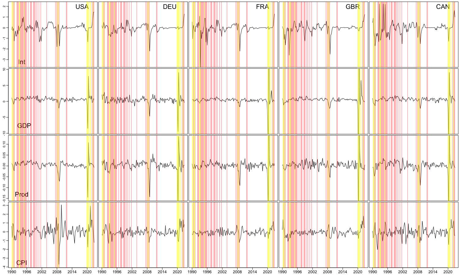
Figure 3: Clustered time series plot of the economic indicators, with phase 1 shaded yellow, phase 2 shaded red, and phase 3 unshaded.

Tables S.8.1 – S.8.9 show the MLE of the parameter matrices $\bm{A}_{k,1},\bm{B}_{k,1}$ and $\bm{C}_{k,1}$ for $k\in\{1,2,3\}$, and the corresponding standard errors, respectively. Due to the identifiablility constraints, the Frobenius norms of $\bm{B}$’s are scaled to 1. To facilitate model interpretation (Chen et al.,, 2021), the signs of the significant coefficient matrix elements, at the 5% level, are displayed on the right side of the tables, specifically, using symbols (+) for positively significant, (-) for negatively significant, and (0) for insignificant coefficients. For instance, the first column of $\bm{A}_{k,1}$ can be understood as the impact of the previous quarter’s interest rates on the current economic indicators, while the first column of $\bm{B}_{k,1}$ captures the influence of US’s last quarter’s indicators on the current quarter’s indicators of all countries, for each $k\in\{1,2,3\}$. The estimated parameter matrices $\hat{\bm{A}}$’s and $\hat{\bm{B}}$’s demonstrate both differences and similarities among different phases. Concerning the differences, one example is that the second column of $\hat{\bm{A}}_{2,1}$ indicates that the GDP growth of the previous quarter has a significantly positive influence on all the economic indicators in the current quarter. However, upon examining the second column of $\hat{\bm{A}}_{3,1}$ , the previous quarter’s GDP growth does not have a significant impact on all the indicators of the current quarter, except for itself. Regrading the similarities, by checking the first columns of $\hat{\bm{B}}$’s, it is observed that the US’s previous quarter’s indicators consistently have a positive effect on current quarter’s indicators from all the countries across the three phases, with only a few exceptions.

Moreover, the out-of-sample prediction performance is also examined. We use the data from Q1 1990 to Q2 2021 ($1\leq t\leq 126$) to fit the model, and derive the one-step marginal predictive distributions for Q3 2021 to Q4 2022 ($127\leq t\leq 132$). The observed values along with the predictive values by the conditional mean are shown in Figures 4 – 5 and Figures S.8.2 – S.8.5. In each plot, the shaded areas indicate the 95% highest density region. The plots display some interesting patterns. The marginal predictive distributions of interest rates and the CPI are generally unimodal or bimodal, while those of GDP growth and industrial production growth are generally bimodal or trimodal. In general, most of the 95% highest density regions capture the true observations.

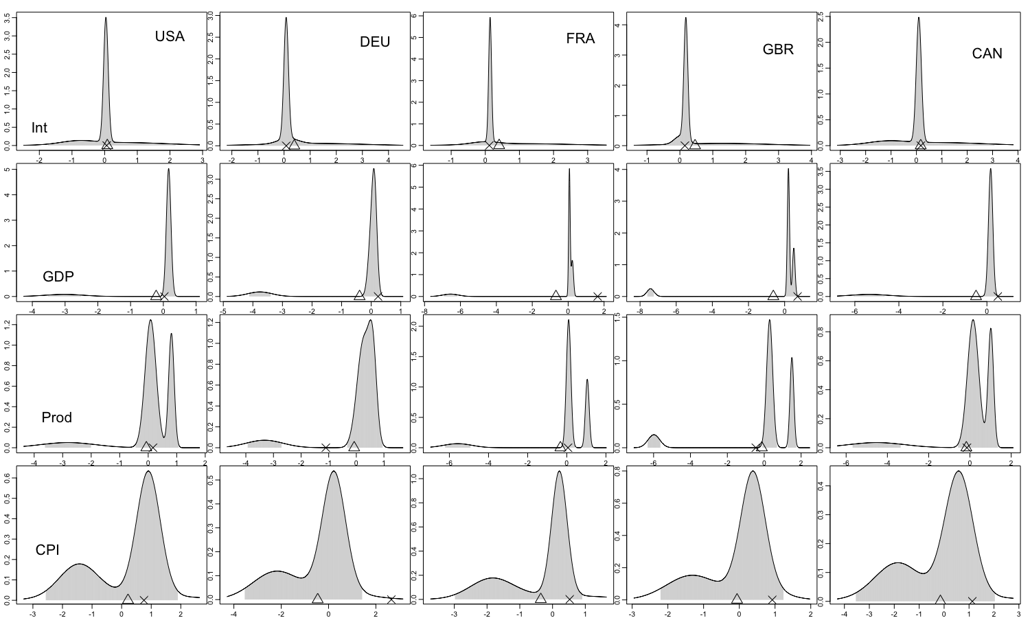
Figure 4: One-step marginal predictive distribution for Q3 2021, with $\times$ representing the observed values and $\triangle$ the predicted values, and the shaded areas representing the 95% highest density interval.

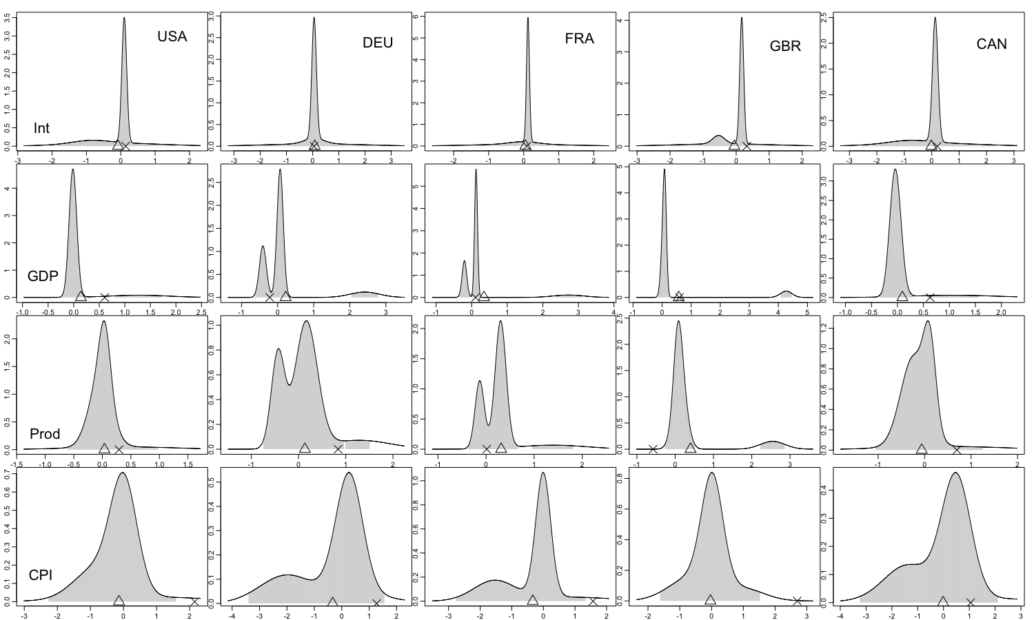
Figure 5: One-step marginal predictive distribution for Q4 2021, with $\times$ representing the observed values and $\triangle$ the predicted values, and the shaded areas representing the 95% highest density interval.

The one-step ahead out-of-sample prediction errors of the MMAR model are compared with the following models:

1. MAR($p$): matrix autoregression, $p\in\{1,2\}$.

2. VAR($p$): vector autoregression, $p\in\{1,2\}$.

We have also attempted to implement the mixture VAR model (Fong et al.,, 2007). However, the estimation process using the EM algorithm did not converge due to a singular variance-covariance matrix error. Additionally, fitting the Gaussian mixture vector autoregressive model (Kalliovirta et al.,, 2016) using the gmvarkit package resulted in errors. The estimation errors suggest that these two models may be inappropriate for analyzing high-dimensional data.

Using the conditional mean for prediction, the mean squared prediction errors (MSPE) are given in Table 6. Although for the mixture models, the conditional expectations may not be optimal for predicting future values, the MMAR model still clearly outperforms the MAR and VAR models.

MMAR(3;1,1,1)	MAR(1)	MAR(2)	VAR(1)	VAR(2)
26.22	50.72	54.13	73.10	134.64

Table 6: Mean of squared out-of-sample prediction errors.

8 Conclusion

We have proposed a new mixture model for matrix-valued time series data, with the capability to effectively capture changing dynamics. We investigate both strict and weak stationarity conditions for the proposed model. An EM algorithm is implemented to estimate the MLE of the parameters, and the asymptotic properties of the MLE are derived. Based on our simulation results, we recommend using either the BIC or the GIC for model selection.

There are several directions to extend the proposed MMAR model. The conditional matrix normal distribution in the model may be replaced by other distributions, such as matrix-valued t-distributions or even some skewed matrix-valued distributions (Gallaugher and McNicholas,, 2018). These models are potentially useful for modeling matrix-valued financial data with heavy tails, such as the Fama-French portfolios cross-classified by size and book-to-market ratio. Also, a Markov switching model can be developed for matrix-valued time series data. Moreover, it is important to note that the proposed MMAR model may contain a large number of parameters, particularly with high-dimensional matrix time series and numerous mixture components with high autoregressive orders. A promising solution to the aforementioned problem is to assume that the parameter matrices $\bm{A}$’s and $\bm{B}$’s are of low ranks, resulting in a reduced-rank MMAR model. In addition, when dealing with high-dimensional matrix-valued time series data, regularization methods can be applied to promote sparsity. These regularization methods can also be applied to the variance-covariance matrices. We may also assume that variance-covariance matrices admit some low rank structures, which can be represented by the sum of a diagonal matrix and a low rank matrix.

SUPPLEMENTAL MATERIALS

The Supplemental Materials contains the proofs of the theorems and additional results for the simulation studies and the real application.

Supplemental Materials of “Mixture Matrix-valued Autoregressive Model”

The Supplemental Materials are organized as follows. Section S.1 gives the proofs the propositions in section 3, which are related to the stationarity and ergodicity of the MMAR model. Section S.2 lists some preliminaries for the proofs of the theorems. Section S.3 and Section S.4 gives the proofs of Theorem 1 and Theorem 2, respectively. Section S.5 and Section S.6 collects the proofs of some lemmas. Section S.7 presents some additional simulations, and Section S.8 shows some additional results for the real data analysis.

S.1 Proofs of the Propositions in Section 3

The strict and weak stationary conditions of the SDE model (13) are given by the following two theorems, respectively.

Theorem S.1.1 (Theorem 4.27 in Douc et al., 2014).

In model (13), let $\{(\bm{D}_{t},\bm{\eta}_{t})\}$ be a sequence of strictly stationary and ergodic sequence. Assume that,

$$\mathbb{E}{\left(\log^{+}\|\bm{D}_{1}\|\right)}<\infty~{}~{}~{}~{}and~{}~{}~{}~{}\mathbb{E}{\left(\log^{+}\|\bm{\eta}_{0}\|\right)}<\infty.$$

Also assume that its top-Lyapunov exponent $\gamma$, defined in (15), is strictly negative. Then,

$$\tilde{\mathcal{X}_{t}}=\sum_{j=0}^{\infty}\left(\prod_{i=t-j+1}^{t}\bm{D}_{i}\right)\bm{\eta}_{t-j}$$ (S.1.1)

is the unique strictly stationary solution to equation (13).

Theorem S.1.2 (Theorem 4.30 in Douc et al., 2014).

Let $q\geq 1$ and $\{(\bm{D}_{t},\bm{\eta}_{t})\}$ be a sequence of i.i.d. random elements, such that the $q$th norm Lyapunov coefficient is strictly negative, and $\mathbb{E}{\left(\|\bm{\eta}_{0}\|^{q}\right)}<\infty$. Then equation (13) has a unique strictly stationary solution $\tilde{\mathcal{X}_{t}}$ given in (S.1.1), such that $\mathbb{E}{\left(\|\tilde{\mathcal{X}_{t}}\|^{q}\right)}<\infty$. Moreover, the right-hand-side of (17) converges in the $q$th norm.

The Fekete’s sub-additive lemma can be used to derive an equivalent expression of $\gamma_{q}$ given in Equation (16).

Lemma S.1.1 (Fekete’s Subadditive Lemma).

Let $\{a_{t},t\geq 1\}$ be a sequence, such that $\forall t_{1},t_{2}\in\mathbb{N}^{*}$, $a_{t_{1}+t_{2}}\leq a_{t_{1}}+a_{t_{2}}$. Then,

$$\lim_{t\to\infty}\frac{a_{t}}{t}=\inf_{t\in\mathbb{N}^{*}}\frac{a_{t}}{t}.$$

Proof of Equation (16).

By definition, matrix norms enjoys the property of sub-multiplicative (Horn and Johnson,, 2012, pp. 341). That is to say, for any matrices $\bm{M}_{1}$ and $\bm{M}_{2}$ such that $\bm{M}_{1}\bm{M}_{2}$ is well-defined,

$$\|\bm{M}_{1}\bm{M}_{2}\|\leq\|\bm{M}_{1}\|\|\bm{M}_{2}\|.$$

Assume $\{\bm{D}_{t}\}$ is a sequence of i.i.d. random matrices. Let $a_{t}=\log\left\{\mathbb{E}{\left(\|\bm{D}_{t}\bm{D}_{t-1}\dots\bm{D}_{1}\|^{q}\right)}\right\}^{1/q}$. For any $t_{1},t_{2}\in\mathbb{N}^{*}$,

$$\|\bm{D}_{t_{1}+t_{2}}\bm{D}_{t_{1}+t_{2}-1}\dots\bm{D}_{1}\|^{q}\leq\|\bm{D}_{t_{1}+t_{2}}\dots\bm{D}_{t_{1}+1}\|^{q}\cdot\|\bm{D}_{t_{1}}\dots\bm{D}_{1}\|^{q}.$$

By independence,

$$\mathbb{E}{\left(\|\bm{D}_{t_{1}+t_{2}}\bm{D}_{t_{1}+t_{2}-1}\dots\bm{D}_{1}\|^{q}\right)}\leq\mathbb{E}{\left(\|\bm{D}_{t_{1}+t_{2}}\dots\bm{D}_{t_{1}+1}\|^{q}\right)}\cdot\mathbb{E}{\left(\|\bm{D}_{t_{1}}\dots\bm{D}_{1}\|^{q}\right)},$$

and hence,

$$a_{t_{1}+t_{2}}\leq a_{t_{1}}+a_{t_{2}}.$$

Therefore,

$$\gamma_{q}=\lim_{t\to\infty}\frac{1}{t}\log\mathbb{E}^{1/q}\left(\|\bm{D}_{t}\dots\bm{D}_{1}\|^{q}\right)=\inf_{t\in\mathbb{N}^{*}}\frac{1}{t}\log\mathbb{E}^{1/q}\left(\|\bm{D}_{t}\dots\bm{D}_{1}\|^{q}\right).$$

∎

The proofs of the propositions in Section 3 are given below.

Proof of Proposition 1.

Under condition (14), it follows that,

$$\mathbb{E}{\left(\log^{+}\|\bm{D}_{1}\|\right)}=\sum_{k=1}^{K}\alpha_{k}\log^{+}(\|\bm{\Phi}_{k}\|)<\infty,$$

and $\mathbb{E}{\left(\log^{+}\|\bm{\eta}_{0}\|\right)}<\infty$ because of normality. By Theorem S.1.1, the results holds. ∎

Proof of Proposition 2.

First notice that $\{\mathcal{X}_{t}\}$ is a time homogeneous Markov chain, as it is strictly stationary and its unique stationary solution is given by (17). Define the transition kernel by,

$$\mathrm{P}(\mathcal{X}_{t},\cdot)=\Pr(\mathcal{X}_{t+1}\in\cdot|\mathcal{X}_{t}),$$

The $1$-step transition density is,

$$f(\mathcal{X}_{t+1}|\mathcal{X}_{t};\bm{\theta})=f(\bm{y}_{t+1}|\mathcal{X}_{t};\bm{\theta})=\sum_{k=1}^{K}f_{t+1}(\bm{y}_{t+1}|\mathcal{X}_{t};\bm{\theta}_{k}),$$

indicating that $f(\mathcal{X}_{t+1}|\mathcal{X}_{t};\bm{\theta})>0$ for all $\mathcal{X}_{t+1}$ and $\mathcal{X}_{t}$. Therefore, the Markov chain $\{\mathcal{X}_{t}\}$ is irreducible and aperiodic. It can be seen that both the $1$-step transition probability and the stationary distribution are equivalent to a Lebesgue measure, hence $\mathrm{P}(\mathcal{X}_{t},\cdot)$ is absolute continuous with respect to the stationary distribution. Also, the initial distribution is absolute continuous with respect to the stationary distribution. By Theorem 1.1 in Chan, (1993), the Markov chain $\{\mathcal{X}_{t}\}$ is ergodic. ∎

Proof of Proposition 3.

Since the MMAR model is a special case of the mixture VAR model with parameter restrictions, let $\bm{B}_{k}\otimes\bm{A}_{k}$ play the role of $\Theta_{k1}$ in Theorem 1 of Fong et al., (2007) and this proposition is proved. ∎

Proof of Proposition 4.

Similar to the proof of Proposition 3, let $\bm{B}_{k}\otimes\bm{A}_{k}$ play the role of $\Theta_{k1}$ in Theorem 3 of Fong et al., (2007) and this Proposition is proved. ∎

Proof of Proposition 5.

Under condition (14), it follows that,

$$\mathbb{E}{\left(\log^{+}\|\bm{D}_{1}\|\right)}=\sum_{k=1}^{K}\alpha_{k}\log^{+}(\|\bm{\Phi}_{k}\|)<\infty,$$

and $\mathbb{E}{\left(\log^{+}\|\bm{\eta}_{0}\|\right)}<\infty$ because of normality. By Theorem S.1.2, the results holds. ∎

S.2 Preliminaries for the Proofs of Theorem 1 and 2

We begin with some notations and properties of matrices. Let $\bm{M}$ be an $m\times n$ matrix and $\bm{M}(g,h)$ be the $(g,h)$-th entry of $\bm{M}$. There exists a commutation matrix $\bm{K}_{m,n}$, such that,

$$\bm{K}_{m,n}\mathrm{vec}{\left(\bm{M}\right)}=\mathrm{vec}{\left(\bm{M}^{\mathsf{T}}\right)}.$$

The commutation matrices enjoy the following interesting properties (Magnus and Neudecker,, 1979):

$$\bm{K}_{m,n}=\bm{K}_{n,m}^{\mathsf{T}},$$ (S.2.1)

$$\bm{K}_{n,m}(\bm{M}_{1}\otimes\bm{M}_{2})\bm{K}_{m,n}=\bm{M}_{2}\otimes\bm{M}_{1},$$ (S.2.2)

where $\bm{M}_{1}\in\mathbb{R}^{m\times m}$ and $\bm{M}_{2}\in\mathbb{R}^{n\times n}$. Let $\bm{P}$ be an arbitrary $m\times m$ positive definite matrix. There exists a unique expansion matrix $\bm{G}_{m}$, such that $\mathrm{vec}{\left(\bm{P}\right)}=\bm{G}_{m}\mathrm{vech}{\left(\bm{P}\right)}$ (Henderson and Searle,, 1979). For an $mn$-vector $\bm{v}$, define the operator $\mathrm{mat}_{m,n}(\bm{v})$ to transfer $\bm{v}$ into an $m\times n$ matrix, such that,

$$\mathrm{vec}{\left(\mathrm{mat}_{m,n}(\bm{v})\right)}=\bm{v}.$$ (S.2.3)

Define

$$\bm{\gamma}_{k}= \big{(}\mathrm{vec}{\left(\bm{A}_{k,1}\right)}^{\mathsf{T}},\mathrm{vec}{\left(\bm{B}_{k,1}\right)}^{\mathsf{T}},\dots,\mathrm{vec}{\left(\bm{A}_{k,p_{k}}\right)}^{\mathsf{T}},\mathrm{vec}{\left(\bm{B}_{k,p_{k}}\right)},$$

$$\mathrm{vec}{\left(\bm{C}_{k}\right)}^{\mathsf{T}},\mathrm{vech}{\left(\bm{U}_{k}^{-1}\right)}^{\mathsf{T}},\mathrm{vech}{\left(\bm{V}_{k}^{-1}\right)}^{\mathsf{T}}\big{)}^{\mathsf{T}}$$

the parameters for the $k$th component without identifiability constraints, and

$$\bm{\gamma}=(\bm{\gamma}_{1}^{\mathsf{T}},\dots,\bm{\gamma}_{K}^{\mathsf{T}},\alpha_{1},\dots,\alpha_{K-1})^{\mathsf{T}}.$$

We also define $\bm{\gamma}^{0}$ the true parameters, as a function of $\bm{\theta}^{0}$. Constraint (8) indicates that,

$$\bm{B}_{k,i}(1,1)=\sqrt{1-\sum_{(g,h)\neq(1,1)}[\bm{B}_{i}(g,h)]^{2}},~{}~{}1\leq k\leq K,~{}1\leq i\leq p_{k},$$

and

$$\bm{V}^{-1}_{i}(1,1)=\sqrt{1-\sum_{g\geq h}[\bm{V}^{-1}_{i}(g,h)]^{2}}.$$

Since it is more convenient to take partial derivatives of the log-likelihood function w.r.t. $\mathrm{vech}{\left(\bm{U}_{k}^{-1}\right)}$ and $\mathrm{vech}{\left(\bm{V}_{k}^{-1}\right)}$, our idea is to first derive the Fisher information matrix w.r.t. $\bm{\gamma}$ , and then use the delta method to derive the Fisher information matrix w.r.t. $\bm{\theta}$. Also, observe that $\mathrm{vech}{\left(\bm{U}_{k}^{-1}\right)}$ and $\mathrm{vech}_{-1}{\left(\bm{V}_{k}^{-1}\right)}$ are bijective functions of $\mathrm{vech}{\left(\bm{U}_{k}\right)}$ and $\mathrm{vech}_{-1}{\left(\bm{V}_{k}\right)}$, respectively. By the chain rule,

$$\frac{\partial l_{t}(\bm{\theta})}{\partial\bm{\theta}}=\frac{\partial\bm{\gamma}^{\mathsf{T}}}{\partial\bm{\theta}}\frac{\partial l_{t}(\bm{\theta})}{\partial\bm{\gamma}}.$$ (S.2.4)

Obviously, $l_{t}(\bm{\theta})=l_{t}(\bm{\gamma})$.

Rao, (1962) established a theorem on the uniform convergence for strictly stationary and ergodic progress. The following version of that theorem is from Straumann and Mikosch, (2006):

Theorem S.2.1 (Theorem 2.7 in Straumann and Mikosch, 2006).

Let $(v_{t})$ be a strictly stationary ergodic sequence of random elements with values in $\mathbb{C}(S,\mathbb{R}^{d^{\prime}})$, where $S\subset\mathbb{R}^{d}$ is a compact set, and $\mathbb{C}(S,\mathbb{R}^{d^{\prime}})$ is the space of continuous $\mathbb{R}^{d^{\prime}}$-valued functions equipped with sup-norm defined as $\sup_{s\in S}|v_{0}(s)|$. Then the uniform strong law of large numbers is implied by $\mathbb{E}{\left(\sup_{s\in S}|v_{0}(s)|<\infty\right)}$.

S.3 Proof of Theorem 1

Proof.

The following two conditions are required for strong consistency,

$$\text{uniform convergence:}~{}~{}\sup_{\bm{\theta}\in\Theta}|L_{T}(\bm{\theta})/(T-p_{\max})-\mathbb{E}{\left(l_{t}(\bm{\theta})\right)}|\overset{a.s.}{\to}0,$$ (S.3.1)

$$\text{well separation:}~{}~{}\sup_{\bm{\theta}:\|\bm{\theta}-\bm{\theta}^{0}\|_{F}\geq\epsilon}\mathbb{E}{\left(l_{t}(\bm{\theta})\right)}<\mathbb{E}{\left(l_{t}(\bm{\theta}^{0})\right)},~{}~{}\forall\epsilon>0.$$ (S.3.2)

The proofs follows the ideas in Kalliovirta et al., (2016). First notice that $\{l_{t}(\bm{\theta})\}$ is also a strictly stationary and ergodic process. By Theorem S.2.1, it suffices to show that $\mathbb{E}{\left(\sup_{\bm{\theta}\in\Theta}|l_{t}(\bm{\theta})|\right)}<\infty$. Since the parameter space $\Theta$ is compact and $\bm{U}_{k}$ and $\bm{V}_{k}$ are positive definite, we have $c_{1}\leq\det(\bm{V}_{k}\otimes\bm{U}_{k})\leq C_{1}$ and $c_{2}\leq\alpha_{k}\leq C_{2}$ for each $k\in\{1,\dots,K\}$, where $0<c_{1}<C_{1}<\infty$ and $0<c_{2}<C_{2}<1$ are some constants. It follows that,

$$l_{t}(\bm{\theta})=\log\left(\sum_{k=1}^{K}\alpha_{k}f_{t}(\bm{y}_{t}|\mathscr{F}_{t-1};\bm{\theta}_{k})\right) \leq\log\left(\sum_{k=1}^{K}\alpha_{k}\det(2\pi\bm{V}_{k}\otimes\bm{U}_{k})^{-1/2}\right)$$

$$\leq\log\left(KC_{2}(2\pi)^{-mn/2}c_{1}^{-1/2}\right),$$ (S.3.3)

and hence $l_{t}(\bm{\theta})$ is bounded above over $\bm{\theta}\in\Theta$. Since $\Theta$ is compact,

$$\mathrm{vec}{\left(\bm{\epsilon}_{t,k}\right)}^{\mathsf{T}}(\bm{V}_{k}\otimes\bm{U}_{k})^{-1}\mathrm{vec}{\left(\bm{\epsilon}_{t,k}\right)}\leq C_{3}(1+\bm{y}_{t}^{\mathsf{T}}\bm{y}_{t}+\mathcal{X}_{t-1}^{\mathsf{T}}\mathcal{X}_{t-1}),$$

for some constant $C_{3}>0$. Therefore,

$$\sum_{k=1}^{K}\alpha_{k}f_{t}(\bm{y}_{t}|\mathscr{F}_{t-1};\bm{\theta}_{k})\geq Kc_{2}(2\pi)^{-\frac{mn}{2}}C_{1}^{-\frac{1}{2}}\exp\left\{-\frac{1}{2}C_{3}(1+\bm{y}_{t}^{\mathsf{T}}\bm{y}_{t}+\mathcal{X}_{t-1}^{\mathsf{T}}\mathcal{X}_{t-1})\right\},$$

and hence,

$$l_{t}(\bm{\theta})\geq\log(c_{2}K)-\frac{mn}{2}\log(2\pi)-\frac{1}{2}\log(C_{1})-\frac{C_{3}}{2}(1+\bm{y}_{t}^{\mathsf{T}}\bm{y}_{t}+\mathcal{X}_{t-1}^{\mathsf{T}}\mathcal{X}_{t-1}),~{}~{}~{}~{}\forall\bm{\theta}\in\Theta.$$ (S.3.4)

By (S.3) and (S.3.4), we can find a sufficiently large constant $C^{*}$ such that,

$$\sup_{\bm{\theta}\in\Theta}|l_{t}(\bm{\theta})|\leq C^{*}(1+\bm{y}_{t}^{\mathsf{T}}\bm{y}_{t}+\mathcal{X}_{t-1}^{\mathsf{T}}\mathcal{X}_{t-1}).$$

Since $\bm{y}_{t}$ has a finite second-order moment, $\mathbb{E}{\left(\sup_{\bm{\theta}\in\Theta}|l_{t}(\bm{\theta})|\right)}<\infty$. Thus (S.3.1) holds, thanks to Theorem S.2.1.

Let $h_{\bm{\theta}}(\mathcal{X}_{t-1})$, $h_{\bm{\theta}}(\bm{y}_{t}|\mathcal{X}_{t-1})$ and $h_{\bm{\theta}}(\bm{y}_{t},\mathcal{X}_{t-1})$ be the probability density functions of $\bm{y}_{t}$, $\bm{y}_{t}|\mathcal{X}_{t-1}$ and $(\bm{y}_{t},\mathcal{X}_{t-1})$, respectively. It is known that $h_{\bm{\theta}}(\bm{y}_{t}|\mathcal{X}_{t-1})=h_{\bm{\theta}}(\bm{y}_{t}|\mathscr{F}_{t-1})=\sum_{k=1}^{K}\alpha_{k}f_{t}(\bm{y}_{t}|\mathscr{F}_{t-1};\bm{\theta}_{k})$. We first show that $\bm{y}_{t}$ is continuous so that $h_{\bm{\theta}}(\bm{y}_{t})$ is well-defined. Let $\mathcal{L}$ be the Lebesgue measure. For any set $S_{1}\in\mathbb{R}^{\mathrm{dim}(\Theta)}$ such that $\mathcal{L}(S_{1})=0$,

$$\Pr(\bm{y}_{t}\in S_{1})=\mathbb{E}{\left(\Pr(\bm{y}_{t}\in S_{1}|\mathcal{X}_{t-1})\right)}=0.$$

Hence $h_{\bm{\theta}}(\bm{y}_{t})$ is well-define, which indicates that,

$$h_{\bm{\theta}}(\bm{y}_{t})=\int h_{\bm{\theta}}(\bm{y}_{t}|\mathcal{X}_{t-1})\mathrm{d}\mathrm{P}_{\bm{\theta}}(\mathcal{X}_{t-1})$$

Next,

$$\mathbb{E}{\left(l_{t}(\bm{\theta})\right)}-\mathbb{E}{\left(l_{t}(\bm{\theta}^{0})\right)}=\int\left(\int h_{\bm{\theta}^{0}}((\bm{y}_{t}|\mathcal{X}_{t-1}))\log\left(\frac{h_{\bm{\theta}}((\bm{y}_{t}|\mathcal{X}_{t-1}))}{h_{\bm{\theta}^{0}}((\bm{y}_{t}|\mathcal{X}_{t-1}))}\right)\mathrm{d}\bm{y}_{t}\right)\mathrm{d}\mathrm{P}_{\bm{\theta}^{0}}(\mathcal{X}_{t-1}).$$

For each $\mathcal{X}_{t-1}$, the inner integral is the negative of Kullback–Leibler divergence between ${h_{\bm{\theta}^{0}}((\bm{y}_{t}|\mathcal{X}_{t-1}))}$ and ${h_{\bm{\theta}}((\bm{y}_{t}|\mathcal{X}_{t-1}))}$, which is non-positive. Hence $\mathbb{E}{\left(l_{t}(\bm{\theta})\right)}-\mathbb{E}{\left(l_{t}(\bm{\theta}^{0})\right)}=0$ if and only if ${h_{\bm{\theta}^{0}}((\bm{y}_{t}|\mathcal{X}_{t-1}))}={h_{\bm{\theta}}((\bm{y}_{t}|\mathcal{X}_{t-1}))}$ almost everywhere. Since $\|\bm{\theta}-\bm{\theta}^{0}\|_{F}\geq\epsilon$ and the mixture model is identifiable, condition (S.3.2) holds due to the compactness of $\Theta$ and the continuity of $\mathbb{E}{\left(l_{t}(\bm{\theta})\right)}$ as a function of $\bm{\theta}$. Therefore, the MLE is strongly consistent. ∎

S.4 Proof of Theorem 2

We begin with the following lemma, and leave its proof to the next section.

Lemma S.4.1.

Suppose that $\{\bm{y}_{t}\}$ is strictly stationary and ergodic, and the sixth-order moment of $\bm{y}_{t}$ is finite. Then for any $1\leq i\leq K$,

$$\mathbb{E}{\left(\sup_{\bm{\theta}\in\Theta}\Big{\|}\frac{\partial\log f_{t}(\bm{y}_{t}|\mathscr{F}_{t-1};\bm{\theta}_{i})}{\partial\bm{\theta}_{i}}\Big{\|}_{F}\right)}<\infty,$$ (S.4.1)

$$\mathbb{E}{\left(\sup_{\bm{\theta}\in\Theta}\Big{\|}\frac{\partial\log f_{t}(\bm{y}_{t}|\mathscr{F}_{t-1};\bm{\theta}_{i})}{\partial\bm{\theta}_{i}}\frac{\partial\log f_{t}(\bm{y}_{t}|\mathscr{F}_{t-1};\bm{\theta}_{i})}{\partial\bm{\theta}_{i}^{\mathsf{T}}}\Big{\|}_{F}\right)}<\infty,$$ (S.4.2)

$$\mathbb{E}{\left(\sup_{\bm{\theta}\in\Theta}\Big{\|}\frac{\partial^{2}\log f_{t}(\bm{y}_{t}|\mathscr{F}_{t-1};\bm{\theta}_{i})}{\partial\bm{\theta}_{i}\partial\bm{\theta}_{i}^{\mathsf{T}}}\Big{\|}_{F}\right)}<\infty,$$ (S.4.3)

$$\mathbb{E}{\left(\sup_{\bm{\theta}\in\Theta}\Big{\|}\frac{\partial}{\partial\bm{\theta}_{i}^{\mathsf{T}}}\mathrm{vec}{\left(\frac{\partial\log f_{t}(\bm{y}_{t}|\mathscr{F}_{t-1};\bm{\theta}_{i})}{\partial\bm{\theta}_{i}}\frac{\partial\log f_{t}(\bm{y}_{t}|\mathscr{F}_{t-1};\bm{\theta}_{i})}{\partial\bm{\theta}_{i}^{\mathsf{T}}}\right)}\Big{\|}_{F}\right)}<\infty,$$ (S.4.4)

$$\mathbb{E}{\left(\sup_{\bm{\theta}\in\Theta}\Big{\|}\mathrm{vec}{\left(\frac{\partial\log f_{t}(\bm{y}_{t}|\mathscr{F}_{t-1};\bm{\theta}_{i})}{\partial\bm{\theta}_{i}}\frac{\partial\log f_{t}(\bm{y}_{t}|\mathscr{F}_{t-1};\bm{\theta}_{i})}{\partial\bm{\theta}_{i}^{\mathsf{T}}}\right)}\frac{\partial\log f_{t}(\bm{y}_{t}|\mathscr{F}_{t-1};\bm{\theta}_{i})}{\partial\bm{\theta}_{i}^{\mathsf{T}}}\Big{\|}_{F}\right)}<\infty,$$ (S.4.5)

$$\mathbb{E}{\left(\sup_{\bm{\theta}\in\Theta}\Big{\|}\frac{\partial}{\partial\bm{\theta}_{i}^{\mathsf{T}}}\mathrm{vec}{\left(\frac{\partial^{2}\log f_{t}(\bm{y}_{t}|\mathscr{F}_{t-1};\bm{\theta}_{i})}{\partial\bm{\theta}_{i}\bm{\theta}_{i}^{\mathsf{T}}}\right)}\Big{\|}_{F}\right)}<\infty,$$ (S.4.6)

$$\mathbb{E}{\left(\sup_{\bm{\theta}\in\Theta}\Big{\|}\mathrm{vec}{\left(\frac{\partial^{2}\log f_{t}(\bm{y}_{t}|\mathscr{F}_{t-1};\bm{\theta}_{i})}{\partial\bm{\theta}_{i}\bm{\theta}_{i}^{\mathsf{T}}}\right)}\frac{\partial\log f_{t}(\bm{y}_{t}|\mathscr{F}_{t-1};\bm{\theta}_{i})}{\partial\bm{\theta}_{i}^{\mathsf{T}}}\Big{\|}_{F}\right)}<\infty.$$ (S.4.7)

Proof of Theorem 2.

Let $\dot{L}_{T}(\bm{\theta})=\frac{\partial}{\partial\bm{\theta}}L_{T}(\bm{\theta})$ and $\mathscr{I}_{T}(\bm{\theta})=-\ddot{L}_{T}(\bm{\theta})=-\frac{\partial^{2}}{\partial\bm{\theta}\partial\bm{\theta}^{\mathsf{T}}}L_{T}(\bm{\theta})$. We use the results in Sweeting, (1980) to prove asymptotic normality. Let $\bm{\Gamma}$ be the matrix $(\bm{\theta}^{(1)},\dots,\bm{\theta}^{(dim(\Theta))})$, where $\bm{\theta}^{(i)}\in\Theta$, $i=1,2,\dots,\mathrm{dim}(\Theta)$. Define $\mathscr{I}_{T}(\bm{\Gamma})$ to be $\mathscr{I}_{T}$ with $i$th row evaluated at $\bm{\theta}^{(i)}$. It suffices to show that,

$$\sup_{\bm{\theta}\in\Theta}\frac{\mathscr{I}_{T}(\bm{\theta})}{T-p_{\max}}\overset{a.s.}{\to}\mathbb{E}{\left(-\ddot{l}_{t}(\bm{\theta})\right)},$$ (S.4.8)

and for all $c>0$,

$$\sup\frac{\|\mathscr{I}_{T}(\bm{\Gamma})-\mathscr{I}_{T}(\bm{\bm{\theta}^{0}})\|_{F}}{T-p_{\max}}\to 0,$$ (S.4.9)

where the sup is over the set $\sqrt{T-p_{\max}}\|\bm{\theta}^{(i)}-\bm{\theta}^{0}\|_{F}\leq c,~{}i=1,2,\dots,\mathrm{dim}(\Theta)$. We first prove (S.4.8). Since $\{\bm{Y}_{t}\}$ is strictly stationary and ergodic, so is $\{\ddot{l}_{t}(\bm{\theta})\}$. By Theorem S.2.1, it suffices to show that $\mathbb{E}{\left(\sup_{\bm{\theta}\in\Theta}\|\ddot{l}_{t}(\bm{\theta})\|_{F}\right)}<\infty$. The first derivatives are,

$$\frac{\partial l_{t}(\bm{\theta})}{\partial\bm{\theta}_{i}} =\frac{1}{\sum_{k=1}^{K}\alpha_{k}f_{t}(\bm{y}_{t}|\mathscr{F}_{t-1};\bm{\theta}_{k})}\frac{\partial\alpha_{i}f_{t}(\bm{y}_{t}|\mathscr{F}_{t-1};\bm{\theta}_{i})}{\partial\bm{\theta}_{i}},~{}~{}1\leq i\leq K,$$

$$\frac{\partial l_{t}(\bm{\theta})}{\partial\alpha_{i}} =\frac{f_{t}(\bm{y}_{t}|\mathscr{F}_{t-1};\bm{\theta}_{i})-f_{t}(\bm{y}_{t}|\mathscr{F}_{t-1};\bm{\theta}_{K})}{\sum_{k=1}^{K}\alpha_{k}f_{t}(\bm{y}_{t}|\mathscr{F}_{t-1};\bm{\theta}_{k})},~{}~{}1\leq i\leq K-1,$$

and the following second derivatives are,

$$\frac{\partial^{2}l_{t}(\bm{\theta})}{\partial\bm{\theta}_{i}\partial\bm{\theta}_{j}^{\mathsf{T}}} =-\frac{1}{\left(\sum_{k=1}^{K}\alpha_{k}f_{t}(\bm{y}_{t}|\mathscr{F}_{t-1};\bm{\theta}_{k})\right)^{2}}\frac{\partial}{\partial\bm{\theta}_{i}}\left(\alpha_{i}f_{t}(\bm{y}_{t}|\mathscr{F}_{t-1};\bm{\theta}_{i})\right)\frac{\partial}{\partial\bm{\theta}_{j}^{\mathsf{T}}}\left(\alpha_{j}f_{t}(\bm{y}_{t}|\mathscr{F}_{t-1};\bm{\theta}_{j})\right)$$

$$+\frac{1}{\sum_{k=1}^{K}\alpha_{k}f_{t}(\bm{y}_{t}|\mathscr{F}_{t-1};\bm{\theta}_{k})}\frac{\partial^{2}}{\partial\bm{\theta}_{i}\partial\bm{\theta}_{j}^{\mathsf{T}}}\left(\alpha_{i}f_{t}(\bm{y}_{t}|\mathscr{F}_{t-1};\bm{\theta}_{i})\right),~{}~{}1\leq i,j\leq K,$$ (S.4.10)

$$\frac{\partial^{2}l_{t}(\bm{\theta})}{\partial\alpha_{i}\partial\alpha_{j}} =\frac{-\left(f_{t}(\bm{y}_{t}|\mathscr{F}_{t-1};\bm{\theta}_{i})-f_{t}(\bm{y}_{t}|\mathscr{F}_{t-1};\bm{\theta}_{K})\right)\left(f_{t}(\bm{y}_{t}|\mathscr{F}_{t-1};\bm{\theta}_{j})-f_{t}(\bm{y}_{t}|\mathscr{F}_{t-1};\bm{\theta}_{K})\right)}{\left(\sum_{k=1}^{K}\alpha_{k}f_{t}(\bm{y}_{t}|\mathscr{F}_{t-1};\bm{\theta}_{k})\right)^{2}},$$

$$~{}\hskip 241.84842pt{1\leq i,j\leq K-1,}$$ (S.4.11)

$$\frac{\partial^{2}l_{t}(\bm{\theta})}{\partial\alpha_{i}\partial\bm{\theta}_{j}} =-\frac{\alpha_{j}\left(f_{t}(\bm{y}_{t}|\mathscr{F}_{t-1};\bm{\theta}_{i})-f_{t}(\bm{y}_{t}|\mathscr{F}_{t-1};\bm{\theta}_{K})\right)\frac{\partial f_{t}(\bm{y}_{t}|\mathscr{F}_{t-1};\bm{\theta}_{j})}{\partial\bm{\theta}_{j}}}{\left(\sum_{k=1}^{K}\alpha_{k}f_{t}(\bm{y}_{t}|\mathscr{F}_{t-1};\bm{\theta}_{k})\right)^{2}}$$

$$+\frac{\frac{\partial}{\partial\bm{\theta}_{j}}\left(f_{t}(\bm{y}_{t}|\mathscr{F}_{t-1};\bm{\theta}_{i})-f_{t}(\bm{y}_{t}|\mathscr{F}_{t-1};\bm{\theta}_{K})\right)}{\sum_{k=1}^{K}\alpha_{k}f_{t}(\bm{y}_{t}|\mathscr{F}_{t-1};\bm{\theta}_{k})},~{}~{}1\leq i\leq K-1,1\leq j\leq K.$$

Also notice that,

$$\frac{\partial f_{t}(\bm{y}_{t}|\mathscr{F}_{t-1};\bm{\theta}_{i})}{\partial\bm{\theta}_{i}} =f_{t}(\bm{y}_{t}|\mathscr{F}_{t-1};\bm{\theta}_{i})\frac{\partial\log f_{t}(\bm{y}_{t}|\mathscr{F}_{t-1};\bm{\theta}_{i})}{\partial\bm{\theta}_{i}},$$ (S.4.13)

$$\frac{\partial^{2}f_{t}(\bm{y}_{t}|\mathscr{F}_{t-1};\bm{\theta}_{i})}{\partial\bm{\theta}_{i}\partial\bm{\theta}_{i}^{\mathsf{T}}} =f_{t}(\bm{y}_{t}|\mathscr{F}_{t-1};\bm{\theta}_{i})\frac{\partial\log f_{t}(\bm{y}_{t}|\mathscr{F}_{t-1};\bm{\theta}_{i})}{\partial\bm{\theta}_{i}}\frac{\partial\log f_{t}(\bm{y}_{t}|\mathscr{F}_{t-1};\bm{\theta}_{i})}{\partial\bm{\theta}_{i}^{\mathsf{T}}}$$

$$+f_{t}(\bm{y}_{t}|\mathscr{F}_{t-1};\bm{\theta}_{i})\frac{\partial^{2}\log f_{t}(\bm{y}_{t}|\mathscr{F}_{t-1};\bm{\theta}_{i})}{\partial\bm{\theta}_{i}\partial\bm{\theta}_{i}^{\mathsf{T}}}.$$ (S.4.14)

Since $c_{2}\leq\alpha_{k}\leq C_{2}$ for each $k$, and

$$0<\frac{\alpha_{i}f_{t}(\bm{y}_{t}|\mathscr{F}_{t-1};\bm{\theta}_{i})}{\sum_{k=1}^{K}\alpha_{k}f_{t}(\bm{y}_{t}|\mathscr{F}_{t-1};\bm{\theta}_{k})}<1,$$ (S.4.15)

we have,

$$\Big{|}\frac{f_{t}(\bm{y}_{t}|\mathscr{F}_{t-1};\bm{\theta}_{i})}{\sum_{k=1}^{K}\alpha_{k}f_{t}(\bm{y}_{t}|\mathscr{F}_{t-1};\bm{\theta}_{k})}\Big{|}=\frac{1}{\alpha_{i}}\Big{|}\frac{\alpha_{i}f_{t}(\bm{y}_{t}|\mathscr{F}_{t-1};\bm{\theta}_{i})}{\sum_{k=1}^{K}\alpha_{k}f_{t}(\bm{y}_{t}|\mathscr{F}_{t-1};\bm{\theta}_{k})}\Big{|}\leq\frac{1}{c_{2}},~{}~{}1\leq i\leq K,$$ (S.4.16)

and

$$\Big{|}\frac{f_{t}(\bm{y}_{t}|\mathscr{F}_{t-1};\bm{\theta}_{i})-f_{t}(\bm{y}_{t}|\mathscr{F}_{t-1};\bm{\theta}_{K})}{\sum_{k=1}^{K}\alpha_{k}f_{t}(\bm{y}_{t}|\mathscr{F}_{t-1};\bm{\theta}_{k})}\Big{|}\leq\frac{1}{c_{2}},~{}~{}1\leq i\leq K-1.$$ (S.4.17)

By (S.4.13)–(S.4.17), the follow inequalities hold:

$$\Big{\|}\frac{\partial^{2}l_{t}(\bm{\theta})}{\partial\bm{\theta}_{i}\partial\bm{\theta}_{i}^{\mathsf{T}}}\Big{\|}_{F} \leq 2\Big{\|}\frac{\partial\log f_{t}(\bm{y}_{t}|\mathscr{F}_{t-1};\bm{\theta}_{i})}{\partial\bm{\theta}_{i}}\frac{\partial\log f_{t}(\bm{y}_{t}|\mathscr{F}_{t-1};\bm{\theta}_{i})}{\partial\bm{\theta}_{i}^{\mathsf{T}}}\Big{\|}_{F}+\Big{\|}\frac{\partial^{2}\log f_{t}(\bm{y}_{t}|\mathscr{F}_{t-1};\bm{\theta}_{i})}{\partial\bm{\theta}_{i}\partial\bm{\theta}_{i}^{\mathsf{T}}}\Big{\|}_{F},$$

$$\Big{|}\frac{\partial^{2}l_{t}(\bm{\theta})}{\partial\alpha_{i}\partial\alpha_{j}}\Big{|} \leq\frac{1}{c_{2}^{2}},$$

$$\Big{\|}\frac{\partial^{2}l_{t}(\bm{\theta})}{\partial\alpha_{i}\partial\bm{\theta}_{i}}\Big{\|}_{F} \leq\frac{2}{c_{2}}\Big{\|}\frac{\partial\log f_{t}(\bm{y}_{t}|\mathscr{F}_{t-1};\bm{\theta}_{i})}{\partial\bm{\theta}_{i}}\Big{\|}_{F}.$$

By lemma S.4.1, it follows that $\mathbb{E}{\left(\sup_{\bm{\theta}\in\Theta}\|\ddot{l}_{t}(\bm{\theta})\|_{F}\right)}<\infty$, and hence (S.4.8) is proved.
Next we prove (S.4.9). Let $\mathscr{I}_{T}^{[i]}(\bm{\theta})$ be the $i$th row of $\mathscr{I}_{T}(\bm{\theta})$. If suffice to show that for each $i\in\{1,2\dots,\mathrm{dim}(\Theta)\}$,

$$\sup_{\sqrt{T-p_{\max}}\|\bm{\theta}-\bm{\theta}^{0}\|_{F}\leq c}\|\mathscr{I}_{T}^{[i]}(\bm{\theta})-\mathscr{I}_{T}^{[i]}(\bm{\theta}^{0})\|_{F}/(T-p_{\max})\to 0.$$

The above condition holds, if

$$\sup_{\sqrt{T-p_{\max}}\|\bm{\theta}-\bm{\theta}^{0}\|_{F}\leq c}\|\mathscr{I}_{T}(\bm{\theta})-\mathscr{I}_{T}(\bm{\theta}^{0})\|_{F}/(T-p_{\max})\to 0.$$

By mean value inequality,

$$\sup_{\sqrt{T-p_{\max}}\|\bm{\theta}-\bm{\theta}^{0}\|_{F}\leq c}\frac{\|\mathscr{I}_{T}(\bm{\theta})-\mathscr{I}_{T}(\bm{\theta}^{0})\|_{F}}{(T-p_{\max})}\leq\sup_{\sqrt{T-p_{\max}}\|\bm{\theta}-\bm{\theta}^{0}\|_{F}\leq c}\|\bm{\theta}-\bm{\theta}^{0}\|_{F}\sup_{\sqrt{T-p_{\max}}\|\bm{\theta}-\bm{\theta}^{0}\|_{F}\leq c}\frac{\|{\partial\mathrm{vec}{\left(\mathscr{I}_{T}(\bm{\theta})\right)}}/{\partial\bm{\theta}^{\mathsf{T}}}\|_{F}}{T-p_{\max}}.$$

Since $\sup_{\sqrt{T-p_{\max}}\|\bm{\theta}-\bm{\theta}^{0}\|_{F}\leq c}\|\bm{\theta}-\bm{\theta}^{0}\|_{F}=o_{p}(1)$, condition (S.4.9) holds if $\frac{\|{\partial\mathrm{vec}{\left(\mathscr{I}_{T}(\bm{\theta})\right)}}/{\partial\bm{\theta}^{\mathsf{T}}}\|_{F}}{(T-p_{\max})}=O_{p}(1)$ uniformly for $\bm{\theta}\subset\Theta$. By Theorem S.2.1, it suffices to show that

$$\mathbb{E}{\left(\sup_{\bm{\theta}\in\Theta}\|{\partial\mathrm{vec}{\left(\ddot{l}(\bm{\theta})\right)}}/{\partial\bm{\theta}^{\mathsf{T}}}\|_{F}\right)}<\infty.$$

The third derivatives are,

$$\frac{\partial^{3}l_{t}(\bm{\theta})}{\partial\alpha_{i}\partial\alpha_{j}\partial\alpha_{g}}= \frac{2\left(f_{t}(\bm{y}_{t}|\mathscr{F}_{t-1};\bm{\theta}_{i})-f_{t}(\bm{y}_{t}|\mathscr{F}_{t-1};\bm{\theta}_{K})\right)}{\left(\sum_{k=1}^{K}\alpha_{k}f_{t}(\bm{y}_{t}|\mathscr{F}_{t-1};\bm{\theta}_{k})\right)^{3}}$$

$$\times\left(f_{t}(\bm{y}_{t}|\mathscr{F}_{t-1};\bm{\theta}_{j})-f_{t}(\bm{y}_{t}|\mathscr{F}_{t-1};\bm{\theta}_{K})\right)\left(f_{t}(\bm{\theta}_{g})-f_{t}(\bm{y}_{t}|\mathscr{F}_{t-1};\bm{\theta}_{K})\right),$$

$$\frac{\partial^{3}l_{t}(\bm{\theta})}{\partial\alpha_{i}\partial\alpha_{j}\partial\bm{\theta}_{g}} =-\frac{\frac{\partial}{\partial\bm{\theta}_{g}}\left\{\left(f_{t}(\bm{y}_{t}|\mathscr{F}_{t-1};\bm{\theta}_{i})-f_{t}(\bm{y}_{t}|\mathscr{F}_{t-1};\bm{\theta}_{K})\right)\left(f_{t}(\bm{y}_{t}|\mathscr{F}_{t-1};\bm{\theta}_{j})-f_{t}(\bm{y}_{t}|\mathscr{F}_{t-1};\bm{\theta}_{K})\right)\right\}}{\left(\sum_{k=1}^{K}\alpha_{k}f_{t}(\bm{y}_{t}|\mathscr{F}_{t-1};\bm{\theta}_{k})\right)^{2}}$$

$$+\frac{2\left(f_{t}(\bm{y}_{t}|\mathscr{F}_{t-1};\bm{\theta}_{i})-f_{t}(\bm{y}_{t}|\mathscr{F}_{t-1};\bm{\theta}_{K})\right)\left(f_{t}(\bm{y}_{t}|\mathscr{F}_{t-1};\bm{\theta}_{j})-f_{t}(\bm{y}_{t}|\mathscr{F}_{t-1};\bm{\theta}_{K})\right)}{\left(\sum_{k=1}^{K}\alpha_{k}f_{t}(\bm{y}_{t}|\mathscr{F}_{t-1};\bm{\theta}_{k})\right)^{3}}\frac{\partial\alpha_{g}f_{t}(\bm{\theta}_{g})}{\partial\bm{\theta}_{g}},$$

$$\frac{\partial^{3}l_{t}(\bm{\theta})}{\partial\bm{\theta}_{i}\partial\bm{\theta}_{j}^{\mathsf{T}}\partial\alpha_{g}} =-\frac{\frac{\partial{(\alpha_{i}\alpha_{j})}}{\partial\alpha_{g}}}{\left(\sum_{k=1}^{K}\alpha_{k}f_{t}(\bm{y}_{t}|\mathscr{F}_{t-1};\bm{\theta}_{k})\right)^{2}}\frac{\partial}{\partial\bm{\theta}_{i}}\left(f_{t}(\bm{y}_{t}|\mathscr{F}_{t-1};\bm{\theta}_{i})\right)\frac{\partial}{\partial\bm{\theta}_{j}^{\mathsf{T}}}\left(f_{t}(\bm{y}_{t}|\mathscr{F}_{t-1};\bm{\theta}_{j})\right)$$

$$+\frac{2f_{t}(\bm{\theta}_{g})-2f_{t}(\bm{y}_{t}|\mathscr{F}_{t-1};\bm{\theta}_{K})}{\left(\sum_{k=1}^{K}\alpha_{k}f_{t}(\bm{y}_{t}|\mathscr{F}_{t-1};\bm{\theta}_{k})\right)^{3}}\frac{\partial}{\partial\bm{\theta}_{i}}\left(\alpha_{i}f_{t}(\bm{y}_{t}|\mathscr{F}_{t-1};\bm{\theta}_{i})\right)\frac{\partial}{\partial\bm{\theta}_{j}^{\mathsf{T}}}\left(\alpha_{j}f_{t}(\bm{y}_{t}|\mathscr{F}_{t-1};\bm{\theta}_{j})\right)$$

$$+\frac{\frac{\partial\alpha_{i}}{\partial\alpha_{g}}}{\sum_{k=1}^{K}\alpha_{k}f_{t}(\bm{y}_{t}|\mathscr{F}_{t-1};\bm{\theta}_{k})}\frac{\partial^{2}f_{t}(\bm{y}_{t}|\mathscr{F}_{t-1};\bm{\theta}_{i})}{\partial\bm{\theta}_{i}\bm{\theta}_{j}^{\mathsf{T}}}$$

$$-\frac{f_{t}(\bm{\theta}_{g})-f_{t}(\bm{y}_{t}|\mathscr{F}_{t-1};\bm{\theta}_{K})}{\left(\sum_{k=1}^{K}\alpha_{k}f_{t}(\bm{y}_{t}|\mathscr{F}_{t-1};\bm{\theta}_{k})\right)^{2}}\frac{\partial^{2}\alpha_{i}f_{t}(\bm{y}_{t}|\mathscr{F}_{t-1};\bm{\theta}_{i})}{\partial\bm{\theta}_{i}\bm{\theta}_{j}^{\mathsf{T}}},$$

$$\frac{\partial}{\partial\bm{\theta}_{g}^{\mathsf{T}}}\mathrm{vec}{\left(\frac{\partial^{2}l_{t}(\bm{\theta})}{\partial\bm{\theta}_{i}\partial\bm{\theta}_{j}^{\mathsf{T}}}\right)} =\frac{-\frac{\partial}{\partial\bm{\theta}_{g}^{\mathsf{T}}}\mathrm{vec}{\left(\frac{\partial}{\partial\bm{\theta}_{i}}\left(\alpha_{i}f_{t}(\bm{y}_{t}|\mathscr{F}_{t-1};\bm{\theta}_{i})\right)\frac{\partial}{\partial\bm{\theta}_{j}^{\mathsf{T}}}\left(\alpha_{j}f_{t}(\bm{y}_{t}|\mathscr{F}_{t-1};\bm{\theta}_{j})\right)\right)}}{\left(\sum_{k=1}^{K}\alpha_{k}f_{t}(\bm{y}_{t}|\mathscr{F}_{t-1};\bm{\theta}_{k})\right)^{2}}$$

$$+\frac{2\mathrm{vec}{\left(\frac{\partial}{\partial\bm{\theta}_{i}}\left(\alpha_{i}f_{t}(\bm{y}_{t}|\mathscr{F}_{t-1};\bm{\theta}_{i})\right)\frac{\partial}{\partial\bm{\theta}_{j}^{\mathsf{T}}}\left(\alpha_{j}f_{t}(\bm{y}_{t}|\mathscr{F}_{t-1};\bm{\theta}_{j})\right)\right)}\frac{\partial\alpha_{g}f_{t}(\bm{\theta}_{g})}{\partial\bm{\theta}_{g}^{\mathsf{T}}}}{\left(\sum_{k=1}^{K}\alpha_{k}f_{t}(\bm{y}_{t}|\mathscr{F}_{t-1};\bm{\theta}_{k})\right)^{3}}$$

$$+\frac{\frac{\partial}{\partial\bm{\theta}_{g}^{\mathsf{T}}}\mathrm{vec}{\left(\frac{\partial^{2}}{\partial\bm{\theta}_{i}\partial\bm{\theta}_{j}^{\mathsf{T}}}\alpha_{i}f_{t}(\bm{y}_{t}|\mathscr{F}_{t-1};\bm{\theta}_{i})\right)}}{\sum_{k=1}^{K}\alpha_{k}f_{t}(\bm{y}_{t}|\mathscr{F}_{t-1};\bm{\theta}_{k})}-\frac{\mathrm{vec}{\left(\frac{\partial^{2}}{\partial\bm{\theta}_{i}\partial\bm{\theta}_{j}^{\mathsf{T}}}\alpha_{i}f_{t}(\bm{y}_{t}|\mathscr{F}_{t-1};\bm{\theta}_{i})\right)}\frac{\partial\alpha_{g}f_{t}(\bm{\theta}_{g})}{\partial\bm{\theta}_{g}^{\mathsf{T}}}}{\left(\sum_{k=1}^{K}\alpha_{k}f_{t}(\bm{y}_{t}|\mathscr{F}_{t-1};\bm{\theta}_{k})\right)^{2}}.$$

By (S.4.13)–(S.4.17), there exists a constant $C_{4}>0$ such that,

$$\Big{|}\frac{\partial^{3}l_{t}(\bm{\theta})}{\partial\alpha_{i}\partial\alpha_{j}\partial\alpha_{g}}\Big{|}\ \leq C_{4},$$

$$\Big{\|}\frac{\partial^{3}l_{t}(\bm{\theta})}{\partial\alpha_{i}\partial\alpha_{i}\bm{\theta}_{i}}\Big{\|}_{F} \leq C_{4}\Big{\|}\frac{\partial\log f_{t}(\bm{y}_{t}|\mathscr{F}_{t-1};\bm{\theta}_{i})}{\partial\bm{\theta}_{i}}\Big{\|}_{F},$$

$$\Big{\|}\frac{\partial^{3}l_{t}(\bm{\theta})}{\partial\bm{\theta}_{i}\partial\bm{\theta}_{i}^{\mathsf{T}}\partial\alpha_{i}}\Big{\|}_{F} \leq C_{4}\Big{\|}\frac{\partial\log f_{t}(\bm{y}_{t}|\mathscr{F}_{t-1};\bm{\theta}_{i})}{\partial\bm{\theta}_{i}}\frac{\partial\log f_{t}(\bm{y}_{t}|\mathscr{F}_{t-1};\bm{\theta}_{i})}{\partial\bm{\theta}_{i}^{\mathsf{T}}}\Big{\|}_{F}$$

$$+C_{4}\Big{\|}\frac{\partial^{2}\log f_{t}(\bm{y}_{t}|\mathscr{F}_{t-1};\bm{\theta}_{i})}{\partial\bm{\theta}_{i}\partial\bm{\theta}_{i}^{\mathsf{T}}}\Big{\|}_{F},$$

$$\frac{1}{C_{4}}\Big{\|}\frac{\partial}{\partial\bm{\theta}_{i}^{\mathsf{T}}}\mathrm{vec}{\left(\frac{\partial^{2}l_{t}(\bm{\theta})}{\partial\bm{\theta}_{i}\partial\bm{\theta}_{i}^{\mathsf{T}}}\right)}\Big{\|}_{F} \leq\Big{\|}\frac{\partial}{\partial\bm{\theta}_{i}^{\mathsf{T}}}\mathrm{vec}{\left(\frac{\partial\log f_{t}(\bm{y}_{t}|\mathscr{F}_{t-1};\bm{\theta}_{i})}{\partial\bm{\theta}_{i}}\frac{\partial\log f_{t}(\bm{y}_{t}|\mathscr{F}_{t-1};\bm{\theta}_{i})}{\partial\bm{\theta}_{i}^{\mathsf{T}}}\right)}\Big{\|}_{F}$$

$$+\Big{\|} \mathrm{vec}{\left(\frac{\partial\log f_{t}(\bm{y}_{t}|\mathscr{F}_{t-1};\bm{\theta}_{i})}{\partial\bm{\theta}_{i}}\frac{\partial\log f_{t}(\bm{y}_{t}|\mathscr{F}_{t-1};\bm{\theta}_{i})}{\partial\bm{\theta}_{i}^{\mathsf{T}}}\right)}\frac{\partial\log f_{t}(\bm{y}_{t}|\mathscr{F}_{t-1};\bm{\theta}_{i})}{\partial\bm{\theta}_{i}^{\mathsf{T}}}\Big{\|}_{F}$$

$$+\Big{\|} \frac{\partial}{\partial\bm{\theta}_{i}^{\mathsf{T}}}\mathrm{vec}{\left(\frac{\partial^{2}\log f_{t}(\bm{y}_{t}|\mathscr{F}_{t-1};\bm{\theta}_{i})}{\partial\bm{\theta}_{i}\bm{\theta}_{i}^{\mathsf{T}}}\right)}\Big{\|}_{F}$$

$$+\Big{\|} \mathrm{vec}{\left(\frac{\partial^{2}\log f_{t}(\bm{y}_{t}|\mathscr{F}_{t-1};\bm{\theta}_{i})}{\partial\bm{\theta}_{i}\bm{\theta}_{i}^{\mathsf{T}}}\right)}\frac{\partial\log f_{t}(\bm{y}_{t}|\mathscr{F}_{t-1};\bm{\theta}_{i})}{\partial\bm{\theta}_{i}^{\mathsf{T}}}\Big{\|}_{F}.$$

By lemma S.4.1, $\mathbb{E}{\left(\sup_{\bm{\theta}\in\Theta}\|{\partial\mathrm{vec}{\left(\ddot{l}(\bm{\theta})\right)}}/{\partial\bm{\theta}^{\mathsf{T}}}\|_{F}\right)}<\infty$, and hence (S.4.9) is proved.
By Theorem 1 and Theorem 2 of Sweeting, (1980),

$$\sqrt{T-p_{\max}}(\hat{\bm{\theta}}-\bm{\theta}^{0})\overset{d}{\to}\mathcal{N}\left(\bm{0},\mathbb{E}^{-1}\left(-\ddot{l}_{t}(\bm{\theta}^{0})\right)\right).$$

∎

S.5 Proof of Lemma S.4.1

Proof.

First notice that $\log\left(f_{t}(\bm{y}_{t}|\mathscr{F}_{t-1};\bm{\gamma}_{i})\right)=\log\left(f_{t}(\bm{y}_{t}|\mathscr{F}_{t-1};\bm{\theta}_{i})\right)$, and

$$\log\left(f_{t}(\bm{y}_{t}|\mathscr{F}_{t-1};\bm{\gamma}_{i})\right)=\frac{-mn}{2}\log(2\pi)-\frac{n}{2}\log\det(\bm{U}_{i})-\frac{m}{2}\log\det(\bm{V}_{i})-\frac{1}{2}\mathrm{tr}{\left[\bm{V}_{i}^{-1}\bm{\epsilon}_{t,i}^{\mathsf{T}}\bm{U}_{i}^{-1}\bm{\epsilon}_{t,i}\right]}.$$ (S.5.1)

For $1\leq i\leq K$ and $1\leq j\leq p_{i}$,

$$\frac{\partial\log f_{t}(\bm{y}_{t}|\mathscr{F}_{t-1};\bm{\gamma}_{i})}{\partial{\mathrm{vec}{\left(\bm{A}_{i,j}\right)}}} =\mathrm{vec}{\left(\bm{U}_{i}^{-1}\bm{\epsilon}_{t,i}\bm{V}_{i}^{-1}\bm{B}_{i,j}\bm{Y}_{t-j}^{\mathsf{T}}\right)},$$ (S.5.2)

$$\frac{\partial\log f_{t}(\bm{y}_{t}|\mathscr{F}_{t-1};\bm{\gamma}_{i})}{\partial{\mathrm{vec}{\left(\bm{B}_{i,j}\right)}}} =\mathrm{vec}{\left(\bm{V}_{i}^{-1}\bm{\epsilon}_{t,i}^{\mathsf{T}}\bm{U}_{i}^{-1}\bm{A}_{i,j}\bm{Y}_{t-j}\right)},$$ (S.5.3)

$$\frac{\partial\log f_{t}(\bm{y}_{t}|\mathscr{F}_{t-1};\bm{\gamma}_{i})}{\partial{\mathrm{vec}{\left(\bm{C}_{i}\right)}}} =\mathrm{vec}{\left(\bm{U}^{-1}_{i}\bm{\epsilon}_{t,i}\bm{V}_{i}^{-1}\right)},$$ (S.5.4)

$$\frac{\partial\log f_{t}(\bm{y}_{t}|\mathscr{F}_{t-1};\bm{\gamma}_{i})}{\partial{\mathrm{vech}{\left(\bm{U}_{i}^{-1}\right)}}} =\frac{n}{2}\bm{G}_{m}^{\mathsf{T}}\mathrm{vec}{\left(\bm{U}_{i}\right)}-\frac{1}{2}\bm{G}_{m}^{\mathsf{T}}\mathrm{vec}{\left(\bm{\epsilon}_{t,i}\bm{V}_{i}^{-1}\bm{\epsilon}_{t,i}^{\mathsf{T}}\right)},$$ (S.5.5)

$$\frac{\partial\log f_{t}(\bm{y}_{t}|\mathscr{F}_{t-1};\bm{\gamma}_{i})}{\partial{\mathrm{vech}{\left(\bm{V}_{i}^{-1}\right)}}} =\frac{m}{2}\bm{G}_{n}^{\mathsf{T}}\mathrm{vec}{\left(\bm{V}_{i}\right)}-\frac{1}{2}\bm{G}_{n}^{\mathsf{T}}\mathrm{vec}{\left(\bm{\epsilon}_{t,i}^{\mathsf{T}}\bm{U}_{i}^{-1}\bm{\epsilon}_{t,i}\right)},$$ (S.5.6)

Each row of each vector on the right-hand-side of (S.5.2) – (S.5.6) is a quadratic polynomial of elements in $(\bm{y}_{t},\mathcal{X}_{t-1})$, whose coefficients are polynomials of elements $\bm{\gamma}_{i}$. Since $\Theta$ is compact, $\bm{\gamma}_{i}$ also belongs to a compact space. Hence there exist a constant $C_{5}$, such that,

$$\Big{\|}\frac{\partial\log f_{t}(\bm{y}_{t}|\mathscr{F}_{t-1};\bm{\theta}_{i})}{\partial{\mathrm{vec}{\left(\bm{A}_{i,j}\right)}}}\Big{\|}\leq C_{5}\left(1+\|\bm{y}_{t}^{\mathsf{T}}\bm{y}_{t}\|+\|\mathcal{X}_{t-1}^{\mathsf{T}}\mathcal{X}_{t-1}\|\right),$$

for all $\bm{\theta}\in\Theta$. Similar upper bounds can be found for $\|\frac{\partial\log f_{t}(\bm{y}_{t}|\mathscr{F}_{t-1};\bm{\theta}_{i})}{\partial{\mathrm{vec}{\left(\bm{B}_{i,j}\right)}}}\|$, $\|\frac{\partial\log f_{t}(\bm{y}_{t}|\mathscr{F}_{t-1};\bm{\theta}_{i})}{\partial{\mathrm{vec}{\left(\bm{C}_{i}\right)}}}\|$, $\|\frac{\partial\log f_{t}(\bm{y}_{t}|\mathscr{F}_{t-1};\bm{\theta}_{i})}{\partial{\mathrm{vech}{\left(\bm{U}_{i}^{-1}\right)}}}\|$ and $\|\frac{\partial\log f_{t}(\bm{y}_{t}|\mathscr{F}_{t-1};\bm{\theta}_{i})}{\partial{\mathrm{vech}{\left(\bm{V}_{i}^{-1}\right)}}}\|$. By chain rule and sub-multiplicity, $\|\frac{\partial\log f_{t}(\bm{y}_{t}|\mathscr{F}_{t-1};\bm{\theta}_{i})}{\partial{\mathrm{vec}_{-1}{\left(\bm{B}_{i,j}\right)}}}\|$, $\|\frac{\partial\log f_{t}(\bm{y}_{t}|\mathscr{F}_{t-1};\bm{\theta}_{i})}{\partial{\mathrm{vech}{\left(\bm{U}_{i}^{-1}\right)}}}\|$ and $\|\frac{\partial\log f_{t}(\bm{y}_{t}|\mathscr{F}_{t-1};\bm{\theta}_{i})}{\partial{\mathrm{vech}_{-1}{\left(\bm{V}_{i}^{-1}\right)}}}\|$ are all bounded below $C_{6}\left(1+\|\bm{y}_{t}^{\mathsf{T}}\bm{y}_{t}\|+\|\mathcal{X}_{t-1}^{\mathsf{T}}\mathcal{X}_{t-1}\|\right)$, where $C_{6}>0$ is a constant. By assumption, $\bm{y}_{t}$ has a finite second-order moment. Hence (S.4.1) is proved.
Also observe that each element in the matrix $\left(\frac{\partial\log f_{t}(\bm{y}_{t}|\mathscr{F}_{t-1};\bm{\theta}_{i})}{\partial\bm{\theta}_{i}}\frac{\partial\log f_{t}(\bm{y}_{t}|\mathscr{F}_{t-1};\bm{\theta}_{i})}{\partial\bm{\theta}_{i}^{\mathsf{T}}}\right)$ is a polynomial of elements in $(\bm{y}_{t},\mathcal{X}_{t-1})$ up to fourth degree, whose coefficient are polynomials of elements in $\bm{\gamma}_{i}$. Since the parameter space is compact and $\bm{y}_{t}$ has finite fourth moment, $\eqref{sup_1_1}$ is proved.
Similarly, each element in each term of lemma S.4.1 is a polynomial of $(\bm{y}_{t},\mathcal{X}_{t-1})$ up to sixth degree, whose coefficients are polynomials of elements in $\bm{\gamma}_{i}$. This completes the proof of lemma S.4.1.

∎

S.6 Proof of Lemma 1

Let $S_{\bm{\theta}}=\frac{\partial l_{t}(\bm{\theta})}{\partial\bm{\theta}}$ be the score function. It suffices to show that, there exists no non-zero $\mathrm{dim}(\bm{\Theta})$-vector $\bm{h}$ such that

$$\Pr\left(\bm{h}^{\mathsf{T}}S_{\bm{\theta}}=0\right)=1.$$ (S.6.1)

By the chain rule,

$$S_{\bm{\theta}}=\frac{\partial l_{t}(\bm{\theta})}{\partial\bm{\theta}}=\frac{\partial\bm{\gamma}^{\mathsf{T}}}{\partial\bm{\theta}}\frac{\partial l_{t}(\bm{\theta})}{\partial\bm{\gamma}}\triangleq\frac{\partial\bm{\gamma}^{\mathsf{T}}}{\partial\bm{\theta}}S_{\bm{\gamma}}.$$

Therefore,

$$\Pr\left(\bm{h}^{\mathsf{T}}S_{\bm{\theta}}=0\right)=1\Leftrightarrow\Pr\left(\bm{h}^{\mathsf{T}}\frac{\partial\bm{\gamma}^{\mathsf{T}}}{\partial\bm{\theta}}S_{\bm{\gamma}}=0\right)=1$$ (S.6.2)

Let $\bm{m}$ be a $\mathrm{dim}(\bm{\gamma})$-vector. Consider the conditions when

$$\Pr\left(\bm{m}^{\mathsf{T}}S_{\bm{\gamma}}=0\right)=1,$$ (S.6.3)

Recall that,

$$\frac{\partial l_{t}(\bm{\gamma}_{i})}{\partial\bm{\gamma}_{i}}=\frac{\alpha_{i}f_{t}(\bm{y}_{t}|\mathscr{F}_{t-1};\bm{\gamma}_{i})}{\sum_{k=1}^{K}\alpha_{k}f_{t}(\bm{y}_{t}|\mathscr{F}_{t-1};\bm{\gamma}_{k})}\frac{\partial\log(f_{t}(\bm{y}_{t}|\mathscr{F}_{t-1};\bm{\gamma}_{i}))}{\partial\bm{\gamma}_{i}},$$

$$\frac{\partial l_{t}(\bm{\gamma}_{i})}{\partial\alpha_{i}}=\frac{f_{t}(\bm{y}_{t}|\mathscr{F}_{t-1};\bm{\gamma}_{i})-f_{t}(\bm{y}_{t}|\mathscr{F}_{t-1};\bm{\gamma}_{K})}{\sum_{k=1}^{K}\alpha_{k}f_{t}(\bm{y}_{t}|\mathscr{F}_{t-1};\bm{\gamma}_{k})},\quad i\in\{1,2,\dots,K-1\}.$$

Let $\bm{m}=(\bm{m}_{1}^{\mathsf{T}},\dots,\bm{m}_{K}^{\mathsf{T}},m^{\alpha}_{1},\dots,m^{\alpha}_{K-1})^{\mathsf{T}}$ and $\mathcal{Y}_{t}=(\bm{y}_{t},\mathcal{X}_{t-1})$. Then,

$$\eqref{sig_cond_}\Leftrightarrow \sum_{i=1}^{K}\alpha_{i}f_{t}(\bm{y}_{t}|\mathscr{F}_{t-1};\bm{\gamma}_{i})\bm{m}_{i}^{\mathsf{T}}\frac{\partial\log(f_{t}(\bm{y}_{t}|\mathscr{F}_{t-1};\bm{\gamma}_{i}))}{\partial\bm{\gamma}_{i}}$$

$$+\sum_{i=1}^{K-1}m^{\alpha}_{i}\left(f_{t}(\bm{y}_{t}|\mathscr{F}_{t-1};\bm{\gamma}_{i})-f_{t}(\bm{y}_{t}|\mathscr{F}_{t-1};\bm{\gamma}_{K})\right)=0,\quad\text{almost~{}~{}surely}$$ (S.6.4)

For any set $\mathcal{S}\subset\mathbb{R}^{\mathrm{dim}(\mathcal{Y}_{t})}$, (S.6.4) is equivalent to,

where $h_{\bm{\gamma}}(\mathcal{Y}_{t})$ is the joint probability density function of $\mathcal{Y}_{t}$. By the arbitrariness of $\mathcal{S}$, (S.6.5) holds if and only if,

$$\sum_{i=1}^{K}\alpha_{i}f_{t}(\bm{y}_{t}|\mathscr{F}_{t-1};\bm{\gamma}_{i})\bm{m}_{i}^{\mathsf{T}}\frac{\partial\log(f_{t}(\bm{y}_{t}|\mathscr{F}_{t-1};\bm{\gamma}_{i}))}{\partial\bm{\gamma}_{i}}$$

$$+\sum_{i=1}^{K-1}m^{\alpha}_{i}\left(f_{t}(\bm{y}_{t}|\mathscr{F}_{t-1};\bm{\gamma}_{i})-f_{t}(\bm{y}_{t}|\mathscr{F}_{t-1};\bm{\gamma}_{K})\right)=0,\quad\forall\mathcal{Y}_{t}\in\mathbb{R}^{\mathrm{dim}(\mathcal{Y}_{t})},$$

$$\Leftrightarrow\sum_{i=1}^{K}q_{i}(\mathcal{Y}_{t};\bm{\gamma}_{i})f_{t}(\bm{y}_{t}|\mathscr{F}_{t-1};\bm{\gamma}_{i})=0,\quad\forall\mathcal{Y}_{t}\in\mathbb{R}^{\mathrm{dim}(\mathcal{Y}_{t})},$$ (S.6.6)

where

$$q_{i}(\mathcal{Y}_{t};\bm{\gamma}_{i})\triangleq\alpha_{i}\bm{m}_{i}^{\mathsf{T}}\frac{\partial\log(f_{t}(\bm{y}_{t}|\mathscr{F}_{t-1};\bm{\gamma}_{i}))}{\partial\bm{\gamma}_{i}}+{m^{\alpha}_{i}},\qquad i\in\{1,\dots,K\},$$

and $m^{\alpha}_{K}\triangleq-{\sum_{i=1}^{K-1}m^{\alpha}_{i}}$. With a little abuse of notations, here $\mathcal{Y}_{t}$ is treated as a real variable. As a function of $\mathcal{Y}_{t}$, $q_{i}(\mathcal{Y}_{t};\bm{\gamma}_{i})f_{t}(\bm{y}_{t}|\mathscr{F}_{t-1};\bm{\gamma}_{i})$ is known as a polynomial-exponential. Identifiability constraints guarantee that,

$$f_{t}(\bm{y}_{t}|\mathscr{F}_{t-1};\bm{\gamma}_{i})\neq f_{t}(\bm{y}_{t}|\mathscr{F}_{t-1};\bm{\gamma}_{j}),\qquad i\neq j.$$ (S.6.7)

Therefore, the set of polynomial-exponential functions $\{q_{i}(\mathcal{Y}_{t};\bm{\gamma}_{i})f_{t}(\bm{y}_{t}|\mathscr{F}_{t-1};\bm{\gamma}_{i})~{}|~{}q_{i}(\mathcal{Y}_{t};\bm{\gamma}_{i})\not\equiv 0\}$ are algebraically independent (Heittokangas and Wen,, 2021). Consequently,

$$\eqref{sig_cond_3}\Leftrightarrow q_{i}(\mathcal{Y}_{t};\bm{\gamma}_{i})\equiv 0,~{}~{}\forall i\in\{1,\dots,K\},$$ (S.6.8)

Let $\bm{m}_{i}=(\bm{m}_{A_{i1}}^{\mathsf{T}},\bm{m}_{B_{i1}}^{\mathsf{T}},\dots,\bm{m}_{A_{ip_{i}}}^{\mathsf{T}},\bm{m}_{B_{ip_{i}}}^{\mathsf{T}}\bm{m}_{C_{i}}^{\mathsf{T}},\bm{m}_{U_{i}}^{\mathsf{T}},\bm{m}_{V_{i}}^{\mathsf{T}})^{\mathsf{T}}$. Then $q_{i}(\mathcal{Y}_{t};\bm{\gamma}_{i})=0$ can be written as,

$$\left(\sum_{j=1}^{p_{i}}\bm{m}_{A_{ij}}^{\mathsf{T}}\frac{\partial\log f_{t}(\bm{y}_{t}|\mathscr{F}_{t-1};\bm{\gamma}_{i})}{\partial{\mathrm{vec}{\left(\bm{A}_{i,j}\right)}}}+\bm{m}_{B_{ij}}^{\mathsf{T}}\frac{\partial\log f_{t}(\bm{y}_{t}|\mathscr{F}_{t-1};\bm{\gamma}_{i})}{\partial{\mathrm{vec}{\left(\bm{B}_{i,j}\right)}}}\right)+\bm{m}_{C_{i}}^{\mathsf{T}}\frac{\partial\log f_{t}(\bm{y}_{t}|\mathscr{F}_{t-1};\bm{\gamma}_{i})}{\partial{\mathrm{vec}{\left(\bm{C}_{i}\right)}}}$$

$$+\bm{m}_{U_{i}}^{\mathsf{T}}\frac{\partial\log f_{t}(\bm{y}_{t}|\mathscr{F}_{t-1};\bm{\gamma}_{i})}{\partial{\mathrm{vec}{\left(\bm{U}_{i}^{-1}\right)}}}+\bm{m}_{V_{i}}^{\mathsf{T}}\frac{\partial\log f_{t}(\bm{y}_{t}|\mathscr{F}_{t-1};\bm{\gamma}_{i})}{\partial{\mathrm{vec}{\left(\bm{V}_{i}^{-1}\right)}}}+\frac{m^{\alpha}_{i}}{\alpha_{i}}=0.$$ (S.6.9)

By (S.5.2)–(S.5.6) and taking the second derivative w.r.t. $\mathrm{vec}{\left(\bm{Y}_{t}\right)}$ for both sides of (S.6.9), we have,

$$\frac{\partial^{2}\bm{m}_{U_{i}}^{\mathsf{T}}\bm{G}_{m}^{\mathsf{T}}\mathrm{vec}{\left(\bm{Y}_{t}\bm{V}_{i}^{-1}\bm{Y}_{t}^{\mathsf{T}}\right)}}{\partial\mathrm{vec}{\left(\bm{Y}_{t}\right)}\partial\mathrm{vec}{\left(\bm{Y}_{t}\right)}^{\mathsf{T}}}+\frac{\partial^{2}\bm{m}_{V_{i}}^{\mathsf{T}}\bm{G}_{n}^{\mathsf{T}}\mathrm{vec}{\left(\bm{Y}_{t}^{\mathsf{T}}\bm{U}_{i}^{-1}\bm{Y}_{t}\right)}}{\partial\mathrm{vec}{\left(\bm{Y}_{t}\right)}\partial\mathrm{vec}{\left(\bm{Y}_{t}\right)}^{\mathsf{T}}}=\bm{0}.$$ (S.6.10)

The first derivative is

$$\frac{\partial\bm{m}_{U_{i}}^{\mathsf{T}}\bm{G}_{m}^{\mathsf{T}}\mathrm{vec}{\left(\bm{Y}_{t}\bm{V}_{i}^{-1}\bm{Y}_{t}^{\mathsf{T}}\right)}}{\partial\mathrm{vec}{\left(\bm{Y}_{t}\right)}}=\left((\bm{V}_{i}^{-1}\bm{Y}_{t}^{\mathsf{T}})\otimes\bm{I}\right)\bm{G}_{m}\bm{m}_{U_{i}}+\bm{K}_{m,n}^{\mathsf{T}}\left(\bm{I}\otimes(\bm{V}_{i}^{-1}\bm{Y}_{t}^{\mathsf{T}})\right)\bm{G}_{m}\bm{m}_{U_{i}}.$$

Since, $\bm{G}_{m}$ is a expansion matrix, $\mathrm{mat}_{m,m}(\bm{G}_{m}\bm{m}_{U_{i}})$ is a symmetric matrix. The second derivative is

$$\frac{\partial^{2}\bm{m}_{U_{i}}^{\mathsf{T}}\bm{G}_{m}^{\mathsf{T}}\mathrm{vec}{\left(\bm{Y}_{t}\bm{V}_{i}^{-1}\bm{Y}_{t}^{\mathsf{T}}\right)}}{\partial\mathrm{vec}{\left(\bm{Y}_{t}\right)}\partial\mathrm{vec}{\left(\bm{Y}_{t}\right)}^{\mathsf{T}}} =\bm{V}_{i}^{-1}\otimes\mathrm{mat}_{m,m}(\bm{G}_{m}\bm{m}_{U_{i}})+\bm{K}_{m,n}^{\mathsf{T}}\left(\mathrm{mat}_{m,m}(\bm{G}_{m}\bm{m}_{U_{i}})\otimes\bm{V}_{i}^{-1}\right)\bm{K}_{m,n}$$

$$=2\bm{V}_{i}^{-1}\otimes\mathrm{mat}_{m,m}(\bm{G}_{m}\bm{m}_{U_{i}}),$$ (S.6.11)

where the last step is due to the properties (S.2.1) and (S.2.2) of the commutation matrices. Similarly,

$$\frac{\partial^{2}\bm{m}_{V_{i}}^{\mathsf{T}}\bm{G}_{n}^{\mathsf{T}}\mathrm{vec}{\left(\bm{Y}_{t}^{\mathsf{T}}\bm{U}_{i}^{-1}\bm{Y}_{t}\right)}}{\partial\mathrm{vec}{\left(\bm{Y}_{t}\right)}\partial\mathrm{vec}{\left(\bm{Y}_{t}\right)}^{\mathsf{T}}}=2\mathrm{mat}_{n,n}(\bm{G}_{n}\bm{m}_{V_{i}})\otimes\bm{U}_{i}^{-1},$$

where $\mathrm{mat}_{n,n}(\bm{G}_{n}\bm{m}_{V_{i}})$ is also a symmetric matrix. Therefore,

$$\eqref{sig_fin_1} \Rightarrow\bm{V}_{i}^{-1}\otimes\mathrm{mat}_{m,m}(\bm{G}_{m}\bm{m}_{U_{i}})+\mathrm{mat}_{n,n}(\bm{G}_{n}\bm{m}_{V_{i}})\otimes\bm{U}_{i}^{-1}=\bm{0}$$

$$\Rightarrow\bm{V}_{i}^{-1}(1,1)\cdot\mathrm{mat}_{m,m}(\bm{G}_{m}\bm{m}_{U_{i}})+(\mathrm{mat}_{n,n}(\bm{G}_{n}\bm{m}_{V_{i}}))(1,1)\cdot\bm{U}_{i}^{-1}=\bm{0}$$

$$\Rightarrow\bm{m}_{U_{i}}=d_{1i}\mathrm{vech}{\left(\bm{U}_{i}^{-1}\right)},\qquad d_{1i}\in\mathbb{R},$$ (S.6.12)

which further implies that (S.6.10) is equivalent to,

$$\bm{m}_{U_{i}}=d_{1i}\mathrm{vech}{\left(\bm{U}_{i}^{-1}\right)},~{}~{}\bm{m}_{V_{i}}=-{d_{1i}}\mathrm{vech}{\left(\bm{V}_{i}^{-1}\right)},\qquad d_{1i}\in\mathbb{R}.$$ (S.6.13)

Under (S.6.13), it follows that

$$\bm{m}_{U_{i}}^{\mathsf{T}}\frac{\partial\log f_{t}(\bm{y}_{t}|\mathscr{F}_{t-1};\bm{\gamma}_{i})}{\partial{\mathrm{vec}{\left(\bm{U}_{i}^{-1}\right)}}}+\bm{m}_{V_{i}}^{\mathsf{T}}\frac{\partial\log f_{t}(\bm{y}_{t}|\mathscr{F}_{t-1};\bm{\gamma}_{i})}{\partial{\mathrm{vec}{\left(\bm{V}_{i}^{-1}\right)}}}$$

$$= \frac{nd_{1i}}{2}\mathrm{vec}{\left(\bm{U}_{i}^{-1}\right)}^{\mathsf{T}}\mathrm{vec}{\left(\bm{U}_{i}\right)}-\frac{1}{2}\mathrm{vec}{\left(\bm{U}_{i}^{-1}\right)}^{\mathsf{T}}\mathrm{vec}{\left(\bm{\epsilon}_{t,i}\bm{V}_{i}^{-1}\bm{\epsilon}_{t,i}^{\mathsf{T}}\right)}$$

$$-\frac{md_{1i}}{2}\mathrm{vec}{\left(\bm{V}_{i}^{-1}\right)}^{\mathsf{T}}\mathrm{vec}{\left(\bm{V}_{i}\right)}+\frac{1}{2}\mathrm{vec}{\left(\bm{V}_{i}^{-1}\right)}\mathrm{vec}{\left(\bm{\epsilon}_{t,i}^{\mathsf{T}}\bm{U}_{i}^{-1}\bm{\epsilon}_{t,i}\right)}$$

$$= \frac{mnd_{1i}}{2}-\mathrm{vec}{\left(\bm{U}_{i}^{-1}\right)}^{\mathsf{T}}(\bm{\epsilon}_{t,i}\otimes\bm{\epsilon}_{t,i})\mathrm{vec}{\left(\bm{V}_{i}^{-1}\right)}-\frac{mnd_{1i}}{2}+\mathrm{vec}{\left(\bm{V}_{i}^{-1}\right)}^{\mathsf{T}}(\bm{\epsilon}_{t,i}^{\mathsf{T}}\otimes\bm{\epsilon}_{t,i}^{\mathsf{T}})\mathrm{vec}{\left(\bm{U}_{i}^{-1}\right)}$$

$$= 0$$ (S.6.14)

Taking the derivatives w.r.t. $\mathrm{vec}{\left(\bm{Y}_{t}\right)}$ and $\mathrm{vec}{\left(\bm{Y}_{t-j}\right)}$ for both sides of (S.6.9) for all $1\leq j\leq p_{i}$ under (S.6.13), we have

$$\frac{\partial^{2}\bm{m}_{A_{ij}}^{\mathsf{T}}\mathrm{vec}{\left(\bm{U}_{i}^{-1}\bm{Y}_{t}\bm{V}_{i}^{-1}\bm{B}_{i,j}\bm{Y}_{t-j}^{\mathsf{T}}\right)}}{\partial\mathrm{vec}{\left(\bm{Y}_{t}\right)}\partial\mathrm{vec}{\left(\bm{Y}_{t-j}\right)}^{\mathsf{T}}}+\frac{\partial^{2}\bm{m}_{B_{ij}}^{\mathsf{T}}\mathrm{vec}{\left(\bm{V}_{i}^{-1}\bm{Y}_{t}^{\mathsf{T}}\bm{U}_{i}^{-1}\bm{A}_{i,j}\bm{Y}_{t-j}\right)}}{\partial\mathrm{vec}{\left(\bm{Y}_{t}\right)}\partial\mathrm{vec}{\left(\bm{Y}_{t-j}\right)}^{\mathsf{T}}}=\bm{0}$$

$$\Leftrightarrow ~{}(\bm{B}_{i,j}^{\mathsf{T}}\bm{V}_{i}^{-1})\otimes((\mathrm{mat}_{m,m}(\bm{m}_{A_{ij}}))^{\mathsf{T}}\bm{U}_{i}^{-1})+((\mathrm{mat}_{m,m}(\bm{m}_{B_{ij}}))^{\mathsf{T}}\bm{V}_{i}^{-1})\otimes(\bm{A}_{i,j}^{\mathsf{T}}\bm{U}_{i}^{-1})$$

$$\Leftrightarrow ~{}\bm{m}_{A_{ij}}=d_{2ij}\mathrm{vec}{\left(\bm{A}_{i,j}\right)},~{}~{}\bm{m}_{B_{ij}}=-d_{2ij}\mathrm{vec}{\left(\bm{B}_{i,j}\right)},\qquad d_{2ij}\in\mathbb{R}$$ (S.6.15)

Under (S.6.15), it follow that

$$\bm{m}_{A_{ij}}^{\mathsf{T}}\frac{\partial\log f_{t}(\bm{y}_{t}|\mathscr{F}_{t-1};\bm{\gamma}_{i})}{\partial{\mathrm{vec}{\left(\bm{A}_{i,j}\right)}}}+\bm{m}_{B_{ij}}^{\mathsf{T}}\frac{\partial\log f_{t}(\bm{y}_{t}|\mathscr{F}_{t-1};\bm{\gamma}_{i})}{\partial{\mathrm{vec}{\left(\bm{B}_{i,j}\right)}}}=0.$$ (S.6.16)

Taking the derivative w.r.t. $\mathrm{vec}{\left(\bm{Y}_{t}\right)}$ for both sides of (S.6.9) under conditions (S.6.13) and (S.6.15), we have

$$(\bm{U}_{i}^{-1}\otimes\bm{V}_{i}^{-1})\bm{m}_{C_{i}}=\bm{0}\Leftrightarrow\bm{m}_{C_{i}}=\bm{0}.$$ (S.6.17)

Under (S.6.13), (S.6.15) and (S.6.17),

$$\eqref{sing_cond_5}\Leftrightarrow m^{\alpha}_{i}=0.$$

If any of $\{d_{1i},d_{2ij}~{}|~{}1\leq i\leq K,1\leq j\leq p_{i}\}$ is non-zero, then for all $\bm{h}$,

$$\bm{h}^{\mathsf{T}}\frac{\partial\bm{\gamma}^{\mathsf{T}}}{\partial\bm{\theta}}\neq\bm{m}^{\mathsf{T}}.$$

Therefore, (S.6.1) holds if and only if $\bm{h}$ is a zero-vector, which completes the proof.

S.7 Additional Simulation Results

Besides Scenarios 1 and 2, we add the following two simulation scenarios.

• Scenario 3: An MMAR(2;2,2) with $(m,n)=(2,3)$.

• Scenario 4: An MMAR(3;1,1,1) with $(m,n)=(4,5)$.

In Scenario 3, the mixing weights are set to be $(\alpha_{1},\alpha_{2})=(0.4,0.6)$, and the parameter matrices are generated similarly to Scenarios 1 and 2. Both components are weakly stationary as $\rho(\bm{\Phi}_{1})=0.8399<1$ and $\rho(\bm{\Phi}_{2})=0.6691<1$, and so is the overall model. In Scenario 4, the mixing weights are set to be $(\alpha_{1},\alpha_{2},\alpha_{3})=(0.1,0.2,0.7)$ with which we can compare the effect of small mixing weights. The first and the third components are stationary as $\rho(\bm{B}_{1,1}\otimes\bm{A}_{1,1})=0.6682$ and $\rho(\bm{B}_{3,1}\otimes\bm{A}_{3,1})=0.6537$. The second component is not stationary as $\rho(\bm{B}_{2,1}\otimes\bm{A}_{2,1})=1.0136$. However, the overall model is stationary. For Scenario 3, we also compare the performance of selecting $K$ when the AR orders are misspecified by setting $p_{\max}=1$. We select the models for $K\in\{1,2,3\}$ in Scenario 3, and $K\in\{1,2,3,4\}$ in Scenario 4. For both scenarios, we select the AR orders up to 3.

	AIC	BIC	HQ	GIC
$T=200$	36.60%	93.60%	78.60%	99.80%
$T=400$	15.80%	97.80%	82.20%	99.80%
$T=800$	16.20%	98.40%	86.40%	100.00%

Table S.7.1: Percentage of correctly selecting $K=2$ in Scenario 3 with the AR orders given.

	AIC	BIC	HQ	GIC
$T=200$	67.20%	66.80%	70.20%	61.20%
$T=400$	62.00%	95.60%	92.60%	95.60%
$T=800$	45.40%	99.20%	97.60%	99.20%

Table S.7.2: Percentage of correctly selecting $K=3$ in Scenario 4 with the AR orders given.

	AIC	BIC	HQ	GIC
$T=200$	2.20%	95.20%	68.20%	99.60%
$T=400$	0.20%	97.40%	56.00%	100.00%
$T=800$	0.00%	86.40%	13.00%	100.00%

Table S.7.3: Percentage of correctly selecting $K=2$ in Scenario 3 with the AR orders misspecified ($p_{\max}$ is set to be 1).

	AIC	BIC	HQ	GIC
$T=200$	60.60%	100.00%	99.80%	100.00%
$T=400$	74.20%	100.00%	100.00%	100.00%
$T=800$	79.60%	100.00%	100.00%	100.00%

Table S.7.4: Percentage of correctly selecting $p_{\max}=2$ in Scenario 3 with the number of components $K$ given.

	AIC	BIC	HQ	GIC
$T=200$	71.80%	93.40%	87.80%	95.60%
$T=400$	38.00%	98.20%	97.60%	98.40%
$T=800$	11.20%	99.60%	99.40%	99.60%

Table S.7.5: Percentage of correctly selecting $p_{\max}=1$ in Scenario 4 with the number of components $K$ given.

The GIC performs well in generally. However, one exception is observed in Scenario 4 with small sample size ($N=200$). In this case, none of these methods achieve a desired level of performance as the percentage of correctly selecting $K$ falls between 60% and 70%. This could be attributed to the influence of the components with small mixing weights. In this case the GIC has the worst performance, indicating that it could be conservative when the true model contains components with small mixing weights.

S.8 Additional Results of Real Data Analysis

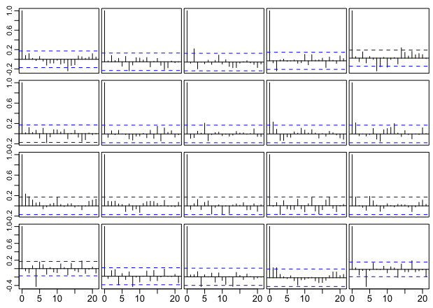
Figure S.8.1: ACF of standardized residuals after fitting MMAR(3,1,1,1) model.

	Int	GDP	Prod	CPI	Int	GDP	Prod	CPI
Int	-1.253 (0.515)	-0.539 (1.202)	0.329 (0.887)	1.351 (0.495)	-	0	0	+
GDP	0.886 (0.239)	4.5 (0.625)	8.251 (0.536)	-0.849 (0.235)	+	+	+	-
Prod	0.46 (0.333)	3.662 (0.838)	4.607 (0.617)	0.459 (0.338)	0	+	+	0
CPI	-1.045 (0.612)	-1.438 (1.479)	2.616 (1.076)	0.7 (0.607)	0	0	+	0

Table S.8.1: The MLE of $\bm{A}_{1,1}$ of the MMAR(3;1,1,1) model, with standard errors given in parentheses.

	USA	DEU	FRA	GBR	CAN	USA	DEU	FRA	GBR	CAN
USA	0.057 (0.03)	-0.089 (0.023)	0.196 (0.025)	-0.12 (0.021)	-0.068 (0.026)	0	-	+	-	-
DEU	0.122 (0.029)	-0.104 (0.023)	0.279 (0.023)	-0.165 (0.02)	-0.155 (0.024)	+	-	+	-	-
FRA	0.124 (0.035)	-0.18 (0.028)	0.384 (0.029)	-0.232 (0.025)	-0.162 (0.03)	+	-	+	-	-
GBR	0.154 (0.024)	-0.236 (0.02)	0.469 (0.026)	-0.297 (0.02)	-0.136 (0.021)	+	-	+	-	-
CAN	0.011 (0.04)	-0.123 (0.03)	0.241 (0.032)	-0.142 (0.026)	-0.032 (0.034)	0	-	+	-	0

Table S.8.2: The MLE of $\bm{B}_{1,1}$ of the MMAR(3;1,1,1) model, with standard errors given in parentheses.

	USA	DEU	FRA	GBR	CAN	USA	DEU	FRA	GBR	CAN
Int	-0.225 (0.342)	0.046 (0.324)	-0.088 (0.4)	0.021 (0.266)	-0.144 (0.441)	0	0	0	0	0
GDP	-0.35 (0.162)	-0.073 (0.154)	-0.378 (0.19)	-0.32 (0.126)	-0.495 (0.208)	-	0	-	-	-
Prod	-0.389 (0.23)	-0.465 (0.216)	-0.63 (0.267)	-0.198 (0.177)	-0.43 (0.296)	0	-	-	0	0
CPI	0.058 (0.411)	0.173 (0.388)	0.364 (0.482)	0.906 (0.319)	0.586 (0.524)	0	0	0	+	0

Table S.8.3: The MLE of $\bm{C}_{1,1}$ of the MMAR(3;1,1,1) model, with standard errors given in parentheses.

	Int	GDP	Prod	CPI	Int	GDP	Prod	CPI
Int	1.695 (0.142)	2.16 (0.271)	-0.539 (0.253)	0.207 (0.146)	+	+	-	0
GDP	0.094 (0.033)	0.233 (0.075)	0.662 (0.077)	-0.076 (0.04)	+	+	+	0
Prod	0.063 (0.048)	0.532 (0.11)	1.331 (0.117)	0.064 (0.056)	0	+	+	0
CPI	-0.153 (0.07)	2.515 (0.197)	-1.414 (0.16)	0.767 (0.09)	-	+	-	+

Table S.8.4: The MLE of $\bm{A}_{2,1}$ of the MMAR(3;1,1,1) model, with standard errors given in parentheses.

	USA	DEU	FRA	GBR	CAN	USA	DEU	FRA	GBR	CAN
USA	0.503 (0.036)	0.056 (0.046)	0.036 (0.053)	0.099 (0.041)	-0.076 (0.045)	+	0	0	+	0
DEU	0.201 (0.069)	0.398 (0.056)	0.062 (0.067)	0.213 (0.053)	0.022 (0.061)	+	+	0	+	0
FRA	0.193 (0.039)	0.291 (0.035)	-0.013 (0.039)	0.228 (0.034)	0.063 (0.036)	+	+	0	+	0
GBR	0.207 (0.06)	-0.024 (0.052)	-0.015 (0.059)	0.366 (0.047)	0.061 (0.054)	+	0	0	+	0
CAN	0.29 (0.074)	0.097 (0.071)	0.027 (0.082)	0.138 (0.064)	0.08 (0.075)	+	0	0	+	0

Table S.8.5: The MLE of $\bm{B}_{2,1}$ of the MMAR(3;1,1,1) model, with standard errors given in parentheses.

	USA	DEU	FRA	GBR	CAN	USA	DEU	FRA	GBR	CAN
Int	-0.094 (0.153)	-0.22 (0.198)	-0.219 (0.116)	-0.281 (0.174)	-0.209 (0.238)	0	0	0	0	0
GDP	0.017 (0.043)	-0.086 (0.055)	-0.006 (0.032)	-0.025 (0.048)	0.008 (0.067)	0	0	0	0	0
Prod	0.014 (0.06)	-0.168 (0.078)	-0.005 (0.045)	0.031 (0.068)	-0.047 (0.093)	0	-	0	0	0
CPI	-0.16 (0.09)	-0.306 (0.116)	-0.118 (0.068)	-0.142 (0.101)	-0.187 (0.139)	0	-	0	0	0

Table S.8.6: The MLE of $\bm{C}_{2,1}$ of the MMAR(3;1,1,1) model, with standard errors given in parentheses.

	Int	GDP	Prod	CPI	Int	GDP	Prod	CPI
Int	1.472 (0.044)	0.347 (0.076)	0.044 (0.064)	0.145 (0.036)	+	+	0	+
GDP	0.302 (0.036)	-0.044 (0.088)	-0.005 (0.074)	-0.01 (0.042)	+	0	0	0
Prod	0.054 (0.053)	-0.072 (0.132)	0.122 (0.11)	0.068 (0.063)	0	0	0	0
CPI	0.251 (0.086)	-0.155 (0.217)	-0.024 (0.181)	0.676 (0.104)	+	0	0	+

Table S.8.7: The MLE of $\bm{A}_{3,1}$ of the MMAR(3;1,1,1) model, with standard errors given in parentheses.

	USA	DEU	FRA	GBR	CAN	USA	DEU	FRA	GBR	CAN
USA	0.511 (0.019)	-0.25 (0.021)	-0.016 (0.027)	0.036 (0.024)	-0.062 (0.023)	+	-	0	0	-
DEU	0.068 (0.024)	0.366 (0.023)	-0.058 (0.026)	-0.115 (0.023)	-0.028 (0.022)	+	+	-	-	0
FRA	0.066 (0.019)	0.139 (0.018)	0.21 (0.02)	-0.115 (0.018)	-0.066 (0.017)	+	+	+	-	-
GBR	0.062 (0.022)	-0.143 (0.019)	0.135 (0.023)	0.236 (0.021)	-0.064 (0.019)	+	-	+	+	-
CAN	0.189 (0.026)	-0.43 (0.02)	0.295 (0.025)	0.104 (0.025)	0.094 (0.026)	+	-	+	+	+

Table S.8.8: The MLE of $\bm{B}_{3,1}$ of the MMAR(3;1,1,1) model, with standard errors given in parentheses.

	USA	DEU	FRA	GBR	CAN	USA	DEU	FRA	GBR	CAN
Int	0.068 (0.031)	0.089 (0.029)	0.125 (0.023)	0.122 (0.026)	0.121 (0.032)	+	+	+	+	+
GDP	0.032 (0.036)	0.038 (0.035)	0.047 (0.028)	0.058 (0.031)	0.052 (0.038)	0	0	0	0	0
Prod	0.033 (0.054)	0.131 (0.052)	0.076 (0.041)	0.001 (0.046)	0.069 (0.057)	0	+	0	0	0
CPI	0.088 (0.088)	0.111 (0.084)	0.038 (0.067)	0 (0.074)	0.047 (0.092)	0	0	0	0	0

Table S.8.9: The MLE of $\bm{C}_{3,1}$ of the MMAR(3;1,1,1) model, with standard errors given in parentheses.

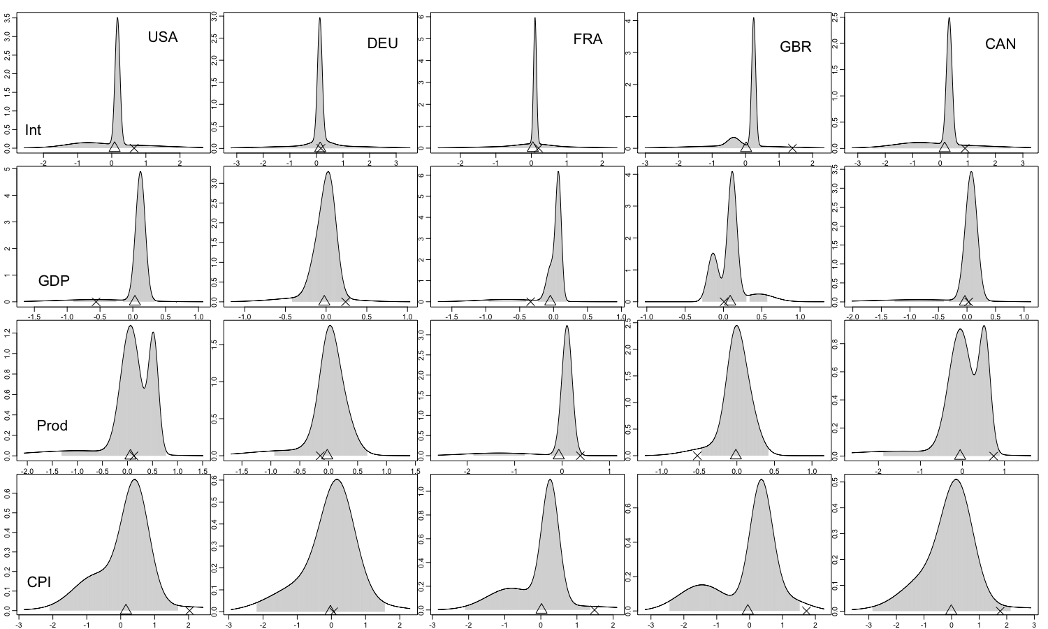
Figure S.8.2: One-step marginal predictive distribution for Q1 2022, with $\times$ representing the observed values and $\triangle$ the predicted values, and the shaded areas representing the 95% highest density interval.

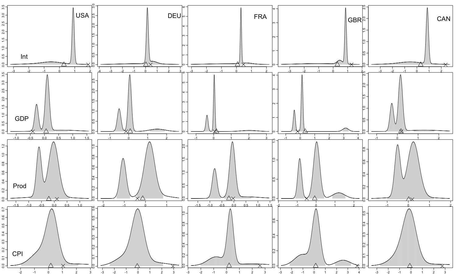
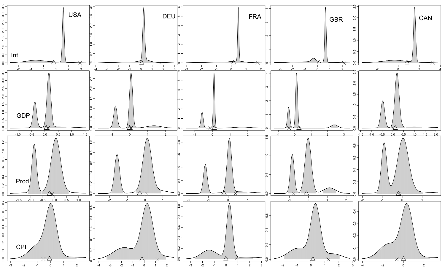
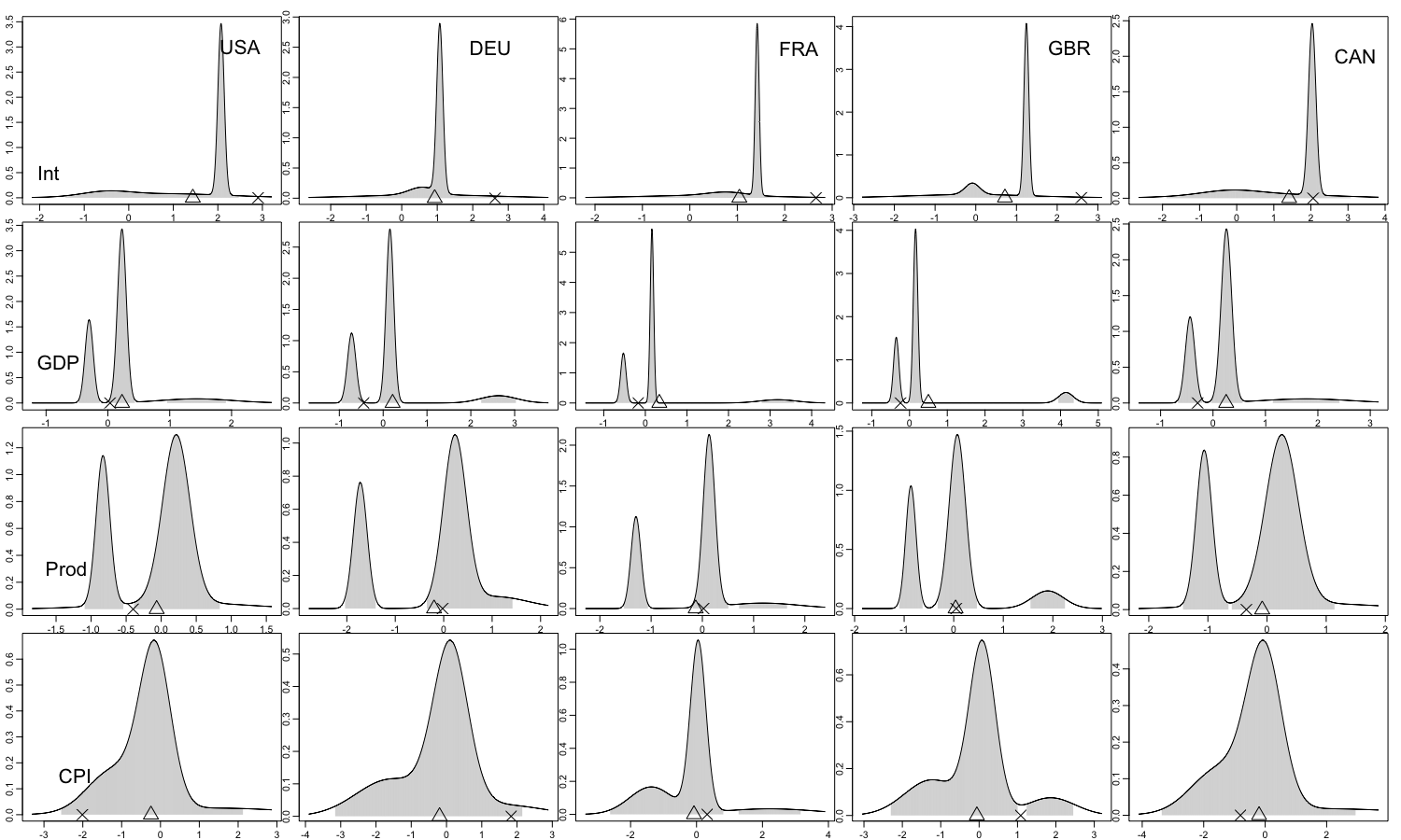
Figure S.8.3: One-step marginal predictive distribution for Q2 2022, with $\times$ representing the observed values and $\triangle$ the predicted values, and the shaded areas representing the 95% highest density interval.

Figure S.8.4: One-step marginal predictive distribution for Q3 2022, with $\times$ representing the observed values and $\triangle$ the predicted values, and the shaded areas representing the 95% highest density interval.

Figure S.8.5: One-step marginal predictive distribution for Q4 2022, with $\times$ representing the observed values and $\triangle$ the predicted values, and the shaded areas representing the 95% highest density interval.

$K$	$p_{\max}$	log-likehood	AIC	BIC	GIC	HQ
1	1	-2492.35	5152.70	5394.22	5574.31	5250.84
1	2	-2376.53	5001.07	5356.64	5699.01	5145.55
1	3	-2286.74	4901.49	5370.50	5895.80	5092.06
2	1	-1753.87	3845.75	4331.66	4881.14	4043.19
2	2	-1728.56	3955.11	4669.13	5631.34	4245.24
2	3	-1743.21	4144.42	5085.30	6501.23	4526.72
3	1	-1504.04	3516.09	4246.39	5236.18	3812.84
3	2	-1421.84	3591.69	4664.15	6350.18	4027.46

Table S.8.10: Model selection for economic indicators dataset.

References

- Basu and Michailidis, (2015) Basu, S. and Michailidis, G. (2015). Regularized estimation in sparse high-dimensional time series models. The Annals of Statistics, 43(4):1535–1567.
- Chan, (1993) Chan, K.-S. (1993). Asymptotic behavior of the gibbs sampler. Journal of the American Statistical Association, 88(421):320–326.
- Chan and Tong, (1990) Chan, K.-S. and Tong, H. (1990). On likelihood ratio tests for threshold autoregression. Journal of the Royal Statistical Society: Series B (Methodological), 52(3):469–476.
- Chang et al., (2022) Chang, J., Zhang, H., Yang, L., and Yao, Q. (2022). Modelling matrix time series via a tensor CP-decomposition. Journal of the Royal Statistical Society. Series B: Statistical Methodology.
- Chen et al., (2021) Chen, R., Xiao, H., and Yang, D. (2021). Autoregressive models for matrix-valued time series. Journal of Econometrics, 222(1):539–560.
- Davies, (1987) Davies, R. B. (1987). Hypothesis testing when a nuisance parameter is present only under the alternative. Biometrika, 74(1):33–43.
- Dempster et al., (1977) Dempster, A. P., Laird, N. M., and Rubin, D. B. (1977). Maximum likelihood from incomplete data via the em algorithm. Journal of the Royal Statistical Society: Series B (Methodological), 39(1):1–22.
- Ding and Cook, (2018) Ding, S. and Cook, R. D. (2018). Matrix variate regressions and envelope models. Journal of the Royal Statistical Society: Series B (Statistical Methodology), 80(2):387–408.
- Douc et al., (2014) Douc, R., Moulines, E., and Stoffer, D. (2014). Nonlinear time series: Theory, methods and applications with R examples. CRC press.
- Fan et al., (2020) Fan, J., Ke, Y., and Wang, K. (2020). Factor-adjusted regularized model selection. Journal of Econometrics, 216(1):71–85.
- Fan and Yao, (2003) Fan, J. and Yao, Q. (2003). Nonlinear time series: nonparametric and parametric methods, volume 20. Springer.
- Fong et al., (2007) Fong, P. W., Li, W. K., Yau, C., and Wong, C. S. (2007). On a mixture vector autoregressive model. Canadian Journal of Statistics, 35(1):135–150.
- Gallaugher and McNicholas, (2018) Gallaugher, M. P. and McNicholas, P. D. (2018). Finite mixtures of skewed matrix variate distributions. Pattern Recognition, 80:83–93.
- Gao et al., (2021) Gao, X., Shen, W., Zhang, L., Hu, J., Fortin, N. J., Frostig, R. D., and Ombao, H. (2021). Regularized matrix data clustering and its application to image analysis. Biometrics, 77(3):890–902.
- Hamilton, (1989) Hamilton, J. D. (1989). A new approach to the economic analysis of nonstationary time series and the business cycle. Econometrica: Journal of the Econometric Society, pages 357–384.
- Han et al., (2021) Han, Y., Zhang, C.-H., and Chen, R. (2021). CP factor model for dynamic tensors. arXiv preprint arXiv:2110.15517.
- Hannan, (1970) Hannan, E. J. (1970). Multiple time series: Wiley series in probability and mathematical statistics. John Wiley and Sons, Inc.(New York).
- Heittokangas and Wen, (2021) Heittokangas, J. M. and Wen, Z.-T. (2021). Generalization of pólya’s zero distribution theory for exponential polynomials, and sharp results for asymptotic growth. Computational Methods and Function Theory, 21:245–270.
- Henderson and Searle, (1979) Henderson, H. V. and Searle, S. (1979). Vec and vech operators for matrices, with some uses in Jacobians and multivariate statistics. Canadian Journal of Statistics, 7(1):65–81.
- Hoff, (2015) Hoff, P. D. (2015). Multilinear tensor regression for longitudinal relational data. The Annals of Applied Statistics, 9(3):1169.
- Horn and Johnson, (2012) Horn, R. A. and Johnson, C. R. (2012). Matrix Analysis. Cambridge university press.
- Hsu et al., (2021) Hsu, N.-J., Huang, H.-C., and Tsay, R. S. (2021). Matrix autoregressive spatio-temporal models. Journal of Computational and Graphical Statistics, 30(4):1143–1155.
- Kalliovirta et al., (2015) Kalliovirta, L., Meitz, M., and Saikkonen, P. (2015). A gaussian mixture autoregressive model for univariate time series. Journal of Time Series Analysis, 36(2):247–266.
- Kalliovirta et al., (2016) Kalliovirta, L., Meitz, M., and Saikkonen, P. (2016). Gaussian mixture vector autoregression. Journal of Econometrics, 192(2):485–498.
- Lam and Yao, (2012) Lam, C. and Yao, Q. (2012). Factor modeling for high-dimensional time series: inference for the number of factors. The Annals of Statistics, pages 694–726.
- Le et al., (1996) Le, N. D., Martin, R. D., and Raftery, A. E. (1996). Modeling flat stretches, bursts outliers in time series using mixture transition distribution models. Journal of the American Statistical Association, 91(436):1504–1515.
- Li and Xiao, (2021) Li, Z. and Xiao, H. (2021). Multi-linear tensor autoregressive models. arXiv preprint arXiv:2110.00928.
- Lu and Zimmerman, (2005) Lu, N. and Zimmerman, D. L. (2005). The likelihood ratio test for a separable covariance matrix. Statistics & Probability Letters, 73(4):449–457.
- Lütkepohl, (2005) Lütkepohl, H. (2005). New introduction to multiple time series analysis. Springer Science & Business Media.
- Magnus and Neudecker, (1979) Magnus, J. R. and Neudecker, H. (1979). The commutation matrix: some properties and applications. The Annals of Statistics, 7(2):381–394.
- Mai et al., (2022) Mai, Q., Zhang, X., Pan, Y., and Deng, K. (2022). A doubly enhanced em algorithm for model-based tensor clustering. Journal of the American Statistical Association, 117(540):2120–2134.
- McLachlan and Peel, (2000) McLachlan, G. and Peel, D. (2000). Finite Mixture Models. Wiley Online Library.
- Meng and Chan, (2022) Meng, J. and Chan, K.-S. (2022). Penalized quasi-likelihood estimation of generalized pareto regression–consistent identification of risk factors for extreme losses. Insurance: Mathematics and Economics, 104:60–75.
- Nicholson et al., (2020) Nicholson, W. B., Wilms, I., Bien, J., and Matteson, D. S. (2020). High dimensional forecasting via interpretable vector autoregression. The Journal of Machine Learning Research, 21(1):6690–6741.
- Nishii, (1984) Nishii, R. (1984). Asymptotic properties of criteria for selection of variables in multiple regression. The Annals of Statistics, pages 758–765.
- Peña et al., (2019) Peña, D., Smucler, E., and Yohai, V. J. (2019). Forecasting multiple time series with one-sided dynamic principal components. Journal of the American Statistical Association.
- Rao, (1962) Rao, R. R. (1962). Relations between weak and uniform convergence of measures with applications. The Annals of Mathematical Statistics, pages 659–680.
- Straumann and Mikosch, (2006) Straumann, D. and Mikosch, T. (2006). Quasi-maximum-likelihood estimation in conditionally heteroscedastic time series: A stochastic recurrence equations approach. The Annals of Statistics, 34(5):2449–2495.
- Sweeting, (1980) Sweeting, T. J. (1980). Uniform asymptotic normality of the maximum likelihood estimator. The Annals of Statistics, pages 1375–1381.
- Tong, (1990) Tong, H. (1990). Non-linear time series: a dynamical system approach. Oxford university press.
- Wang et al., (2021) Wang, D., Zheng, Y., and Li, G. (2021). High-dimensional low-rank tensor autoregressive time series modeling. arXiv preprint arXiv:2101.04276.
- Wong and Li, (2000) Wong, C. S. and Li, W. K. (2000). On a mixture autoregressive model. Journal of the Royal Statistical Society: Series B (Statistical Methodology), 62(1):95–115.