Black Hole Perturbation Theory Meets CFT₂:
Kerr Compton Amplitudes from Nekrasov-Shatashvili Functions

Abstract

We present a novel study of Kerr Compton amplitudes in a partial wave basis in terms of the Nekrasov-Shatashvili (NS) function of the confluent Heun equation (CHE). Remarkably, NS-functions enjoy analytic properties and symmetries that are naturally inherited by the Compton amplitudes. Based on this, we characterize the analytic dependence of the Compton phase-shift in the Kerr spin parameter and provide a direct comparison to the standard post-Minkowskian (PM) perturbative approach within General Relativity (GR). We also analyze the universal large frequency behavior of the relevant characteristic exponent of the CHE – also known as the renormalized angular momentum – and find agreement with numerical computations. Moreover, we discuss the analytic continuation in the harmonics quantum number $\ell$ of the partial wave, and show that the limit to the physical integer values commutes with the PM expansion of the observables. Finally, we obtain the contributions to the tree level, point-particle, gravitational Compton amplitude in a covariant basis through $\mathcal{O}(a_{\text{BH}}^{8})$, without the need to take the super-extremal limit for Kerr spin.

I Introduction

The study of black hole perturbation theory (BHPT) has seen a resurgence in recent years after the observation of the gravitational waves generated by the coalescence of binary black holes Abbott et al. (2016); Akutsu et al. (2021). This revitalization has led to the development of novel perturbative approaches for examining black holes’ responses to external perturbations. These methods draw heavily from Quantum Field Theory (QFT)-inspired techniques, including (quantum) worldline effective field theory (EFT) Goldberger and Rothstein (2006); Rothstein (2014); Goldberger (2022a, b); Porto (2016); Kälin and Porto (2020); Mogull et al. (2021), on-shell amplitudes Cheung et al. (2018); Kosower et al. (2019); Bern et al. (2019, 2020); Buonanno et al. (2022); Cheung et al. (2023); Kosmopoulos and Solon (2023); Bjerrum-Bohr et al. (2022); Brandhuber et al. (2023a); Herderschee et al. (2023); Elkhidir et al. (2023); Georgoudis et al. (2023); Caron-Huot et al. (2023), and the effective-one-body (EOB) approximation Buonanno and Damour (1999, 2000). A crucial aspect of these approaches is to match the physical observables derived from effective models with those calculated in General Relativity (GR), which is key to identifying unknown parameters within the effective theories. Therefore, it is important to exactly solve the differential equations in GR, as well as providing organizing principles to interpret the mathematical results.

This work aims to establish a connection between a novel computational approach to solve the Teukolsky master equation (TME) and the analysis of Compton scattering amplitudes in a Kerr black hole (KBH) background. This computational scheme is grounded in transforming the separated radial and angular components of the TME into a second-order ordinary differential equation (ODE), notably the confluent Heun equation (CHE) Ronveaux (1995). This transformation allows to relate the solutions of the equation to classical Virasoro conformal blocks, as detailed in Bonelli et al. (2022). By exploiting the known analytic properties of these conformal blocks and their representation through the Nekrasov-Shatashvili (NS) special function Nekrasov and Shatashvili (2009), new explicit solutions for the connection coefficients of the CHE could be derived Bonelli et al. (2023). This method has already been applied to the study of physical observables in a variety of gravitational backgrounds including (A)dS black holes Dodelson et al. (2023); Aminov et al. (2023), fuzzballs Bianchi et al. (2022); Bianchi and Di Russo (2023); Bianchi et al. (2023); Giusto et al. (2023), and the astrophysically relevant KBH, with the first application appearing in the context of the exact computation of the spectrum of Quasi Normal Modes Aminov et al. (2022), and more recent approaches to compute greybody factor, Love numbers Bonelli et al. (2022); Consoli et al. (2022) and the study of the post-Newtonian (PN) dynamics in the two-body problem Fucito and Morales (2023).

In this letter, we show that Kerr Compton amplitudes written in a partial wave basis can be directly expressed in terms of the NS-function. As a consequence, the analytic properties of the NS-function translate into sharp statements for the Compton scattering phase-shift. This allows us to:

• Non-perturbatively characterize the polynomial dependence on the KBH spin parameter of different contributions to the phase-shift directly related to the NS-function.

• By comparing to the more traditional method of Mano, Suzuki, and Takasugi (MST) Mano et al. (1996a, b); Mano and Takasugi (1997); Sasaki and Tagoshi (2003), to resum the perturbative – post-Minkowskian (PM) – expansion into exponential functions of derivatives of the NS-function.

• To study analytically the large frequency behaviour of the MST renormalized angular momentum and compare the results to numerical predictions.

By studying the Compton phase-shift in a PM-fashion – namely $\epsilon\equiv 2GM\omega\ll 1$ – we find it naturally separates into a dominating and a depleted contribution. This hierarchical distinction aligns with the “far zone” – conservative, point-particle, leading contribution – and “near-zone” – horizon completion – factorization recently proposed in Ivanov and Zhou (2022); Saketh et al. (2023). The near-far factorization is well defined for harmonics of generic-$\ell$ values, i.e. when analytically continue from $\ell\in\mathbb{N}$ to $\ell\in\mathbb{C}$. This continuation gives rise to apparent divergences once the physical limit $\ell\in\mathbb{N}$ is taken. In an MST language, this manifests as integer $\ell$-poles in the MST coefficients Casals and Ottewill (2015); Casals et al. (2016). In this work we show such poles are spurious and get canceled when adding the PM-expanded near and far zone contributions of the phase-shift together. The final results in this generic$-\ell$ prescription agree with the ones computed in a fixed-$\ell$ prescription, i.e. by solving the ODEs staring with $\ell\in\mathbb{N}$ before PM-expanding Casals and Ottewill (2015); Casals et al. (2016). Therefore, we conclude the PM- and the $\ell$-expansions actually commute. Finally, we provide a new interpretations of the results presented in Bautista et al. (2022) for the higher-spin, tree-level Gravitational Compton amplitude in terms of only far-zone physics, while expanding the state of the art results to eight-order in the Kerr-spin multipole expansion. As mentioned, this far zone computation corresponds to the point-particle limit of the BH, while being purely conservative and polynomial in the KBH spin parameter $\chi$; therefore, no analytic continuation in $\chi$ is required.

II spin-$s$ perturbations off Kerr

The radiative content for perturbation of spin-weight $s$ off a Kerr black hole (KBH) of mass $M$ and spin $a_{\text{BH}}$ is fully encoded in the Teukolsky scalar ${}_{s}\psi$, which solves TME. As shown by Teukolsky’s seminal work Teukolsky (1972, 1973); Teukolsky and Press (1974), ${}_{s}\psi$ admits separation of variables in the frequency domain. Using $(t,r,\vartheta,\varphi)$ as the Boyer-Lindquist coordinates it can be explicitly expressed as

$${}_{s}\psi(t,r,\vartheta,\varphi)=\sum_{\ell m}\int d\omega\,e^{-i\omega t}{}_{s}R_{\ell m}(r){}_{s}S_{\ell m}(\vartheta,\varphi;a_{\text{BH}}\omega)\,.$$ (1)

Here ${}_{s}R_{\ell m}(r)$ solves the radial Teukolksy equation (RTE), whereas ${}_{s}S_{\ell m}(\vartheta,\varphi;a_{\text{BH}}\omega)$ correspond to the spin-weighted spheroidal harmonics. As mentioned above, both the RTE and the angular equation can be reduced to CHE after a suitable change of variables. The RTE has singularities at the inner and outer horizons of the KBH, and at the boundary at infinity. More broadly, Teukolsky equations for a generic class of Type-D space-times correspond to Heun’s equations of certain type, classified by the structure of their singular point Batic and Schmid (2007).

In this work we consider plane wave (PW) perturbations off KBH imposing the physical boundary conditions for the radial function to be purely ingoing at the BH horizon and a superposition of an incoming and a reflected wave at future null infinity (see fig. 2),

$$\begin{split}{}_{s}R^{\rm in}_{\ell m}(r)&=\Delta^{-s}e^{-i\tilde{\omega}r_{*}}\,,\qquad\qquad\qquad\quad r_{*}\to-\infty\,,\\ {}_{s}R^{\rm in}_{\ell m}(r)&={}_{s}B^{\rm inc}_{\ell m}\frac{e^{-i\omega r_{*}}}{r}{+}{}_{s}B^{\rm ref}_{\ell m}\frac{e^{i\omega r_{*}}}{r^{(2s+1)}}\,,\quad r_{*}\to\infty\,.\end{split}$$ (2)

Here $\tilde{\omega}=\omega-\frac{m\chi}{2r_{+}}$ is the co-rotating frequency, $\chi=a_{\text{BH}}/(GM)$ is the dimensionless spin of the KBH, $r_{\pm}=GM(1\pm\kappa)$ are the roots of $\Delta=r^{2}+2GMr+a_{\rm BH}^{2}$, and $\kappa=\sqrt{1-\chi^{2}}$ . The tortoise coordinate $r_{*}$ is determined from the differential equation $\frac{dr_{*}}{dr}=\frac{r^{2}+a_{\text{BH}}^{2}}{\Delta}$ Sasaki and Tagoshi (2003).

The main object of interest is the (Compton) scattering phase-shift which is fully determined from the asymptotic behaviour of the radial functions

$${}_{s}\eta_{\ell m}^{P}e^{2i{}_{s}\delta_{\ell m}^{P}}=(-1)^{\ell+1}\frac{{}_{s}B_{\ell m}^{\text{ref}}}{{}_{s}B_{\ell m}^{\text{inc}}}\times(2\omega)^{2s}A_{s}^{P}~{},$$ (3)

being $A_{s}^{P}$ a function of the Teukolsky-Starobinsky constant (see (49)), with $P$ a parity label. ${}_{s}B^{\rm inc}_{\ell m}$ and ${}_{s}B^{\rm ref}_{\ell m}$ are called connection coefficients of the CHE since they allow us to express a local solution close to a singular point in terms of a local basis of solutions centered around a different singular point. The Heun connection coefficients for generic boundary conditions have been explicitly computed in Bonelli et al. (2023) (see appendix B for a review of the derivation). Using these results we find

$$\frac{{}_{s}B_{\ell m}^{\text{ref}}}{{}_{s}B_{\ell m}^{\text{inc}}}=-i\frac{e^{2i\epsilon(\log(|2\epsilon|)-1/2)}}{|2\omega|^{2s}}e^{\partial_{m_{3}}F-\frac{L}{2}}\frac{\sum_{\sigma=\pm}\frac{\Gamma\left(1{-}2\sigma a\right)\Gamma\left({-}2\sigma a\right)({-}L)^{\sigma a}e^{{-}\frac{\sigma}{2}\partial_{a}F}}{\Gamma\left(\frac{1}{2}{-}\sigma a{+}m_{1}\right)\Gamma\left(\frac{1}{2}{-}\sigma a{+}m_{2}\right)\Gamma\left(\frac{1}{2}{-}\sigma a{+}m_{3}\right)}}{\sum_{\sigma^{\prime}{=}\pm}\frac{\Gamma\left(1{-}2\sigma^{\prime}a\right)\Gamma\left({-}2\sigma^{\prime}a\right)L^{\sigma^{\prime}a}e^{{-}\frac{\sigma^{\prime}}{2}\partial_{a}F}}{\Gamma\left(\frac{1}{2}{-}\sigma^{\prime}a{+}m_{1}\right)\Gamma\left(\frac{1}{2}{-}\sigma^{\prime}a{+}m_{2}\right)\Gamma\left(\frac{1}{2}{-}\sigma^{\prime}a-m_{3}\right)}}\,,$$ (4)

with dictionary of parameters Aminov et al. (2022)

$$m_{1}{=}i\frac{m\chi-\epsilon}{\kappa}\,,\quad m_{2}{=}-s{-}i\epsilon\,,\quad m_{3}{=}i\epsilon{-}s\,,\quad L{=}-2i\epsilon\kappa\,,$$ (5)

$$u=-\lambda-s(s+1)+\epsilon(is\kappa-m\chi)+\epsilon^{2}(2+\kappa)\,,$$

and $\lambda$ the spheroidal eigenvalue. $a$ is implicitly determined from the so called Matone relation Flume et al. (2004); Matone (1995):

$$u=\frac{1}{4}-a^{2}+L\partial_{L}F\left(m_{1},m_{2},m_{3},a,L\right)\,.$$ (6)

All the complexity in computing (4) is then hidden in the special function $F(m_{1},m_{2},m_{3},a,L)$. This is a so called NS-function, and it is given as a convergent series in $L$ whose coefficients are given explicitly in terms of combinatorial formulas (see appendix B for concrete formulas). NS-functions are a class of special functions which appeared for the first time in the context of $\mathcal{N}=2$ supersymmetric gauge theories and Liouville CFT Nekrasov and Shatashvili (2009); Alday et al. (2010). Different NS-functions make their appearance in the connection problem of Heun equations of different types Bonelli et al. (2023). Since in this paper we are only dealing with the CHE, we will not make a notational effort to distinguish the NS-function $F$ from its siblings. From (5), it follows that $L$ acts effectively as a PM-parameter, aligning the $L$ expansion of $F$ with the standard PM-expansion used by the MST method. This observation is crucial and allows for a direct comparison of the two methods as we will see below.

For practical purposes, our strategy to compute (4) is the following:

• compute $F$ up to order $L^{n_{\text{max}}}$,

• invert (6) perturbatively in $L$ to obtain $a(m_{i},u,L)$,

• plug $a(m_{i},u,L)$ back in $F$ and evaluate (4) substituting the dictionary (5) up to order $\epsilon^{n_{\text{max}}}$.

We include the explicit expression for $F$ up to $\mathcal{O}(L^{9})$ in the ancillary files of this work anc . For concreteness, at leading order one finds

$$a=-\frac{\sqrt{(1+2s)^{2}+4\lambda}}{2}+\mathcal{O}(\epsilon)=-\frac{1}{2}-\ell+\mathcal{O}(\epsilon)^{2}\,.$$ (7)

Note that in the $\epsilon\ll 1$ limit $|L|^{a}\sim e^{-(1+2\ell)\log(\epsilon)/2}$, therefore only $\sigma=1$ terms contributes to the sums in (4) at leading order. We call this the far zone contribution. The $\sigma=-1$ terms are thus suppressed by a factor of $|L|^{-2a}\sim\epsilon^{1+2\ell}$, which coincides with the order at which BH horizon effects start to become relevant Page (1976a, b); Saketh et al. (2022, 2023). For this reason, we call the factor containing these terms the near zone. We therefore rewrite formula (4) in the more familiar form

$$\frac{{}_{s}B_{\ell m}^{\text{ref}}}{{}_{s}B_{\ell m}^{\text{inc}}}={{\color[rgb]{0.83984375,0.15234375,0.15625}\underbrace{\frac{e^{2i\epsilon(\log(|2\epsilon|)-1/2)}}{|2\omega|^{2s}}e^{\partial_{m_{3}}F-\frac{L}{2}}e^{i\pi\left(a-\frac{1}{2}\right)}\frac{\Gamma\left(\frac{1}{2}-a-m_{3}\right)}{\Gamma\left(\frac{1}{2}-a+m_{3}\right)}}_{\rm far\,zone}}}\times{{\color[rgb]{0.12109375,0.46484375,0.70703125}\underbrace{\frac{1+e^{-i\pi a}\mathcal{K}}{1+e^{i\pi a}\frac{\cos(\pi(m_{3}-a))}{\cos(\pi(m_{3}+a))}\mathcal{K}}}_{\rm near\,zone}}}~{},$$ (8)

where

$$\mathcal{K}=|L|^{-2a}\frac{\Gamma(2a)\Gamma(2a+1)\Gamma\left(m_{3}-a+\frac{1}{2}\right)\Gamma\left(m_{2}-a+\frac{1}{2}\right)\Gamma\left(m_{1}-a+\frac{1}{2}\right)}{\Gamma(-2a)\Gamma(1-2a)\Gamma\left(m_{3}+a+\frac{1}{2}\right)\Gamma\left(m_{2}+a+\frac{1}{2}\right)\Gamma\left(m_{1}+a+\frac{1}{2}\right)}e^{\partial_{a}F}\,,$$ (9)

thus resembling the near-far factorization proposed in Ivanov and Zhou (2022) for the coefficient-ratio written in the MST-language (see (43) below). The function $\mathcal{K}$ here is called the tidal response function and we shall give a more detailed explanation on it in Appendix A. From the above equation, we observe that the far zone contribution can be written as an analytic functions of $L$ while the near zone is non-analytic in $L$ for generic values of $a$, hence sharing an analog of the analytic structure in $G$ discussed in Saketh et al. (2023). A detailed comparison with MST method will be done in the next section.

III NS-Function, MST PM-Resummation, and the High Frequency limit

Since the phase-shift (3) depends on the NS-function via the connection formula (8), the symmetry properties of $F$ are naturally imprinted in the Compton scattering amplitudes. We start this section then by presenting some properties of the NS-function (see appendix B for conventions and derivations).

Properties of the NS-function— The function

$$\tilde{F}(m_{1},m_{2},m_{3},a,L)=F(m_{1},m_{2},m_{3},a,L)-\frac{m_{3}L}{2}$$ (10)

is invariant under permutations of $(m_{1},m_{2},m_{3})$ and under the reflection $(m_{i},L)\to(-m_{i},-L)$. Accordingly, it only depends on combinations that are left invariant under such transformations, that is

$$(m_{1}m_{2}m_{3})L\,,\,\,(m_{1}m_{2}m_{3})^{2}\,,\,\,L^{2}\,,\,\,\sum_{i=1}^{3}m_{i}^{2n}\,,$$ (11)

$$\,\quad(m_{1}m_{2})^{2n}+(m_{2}m_{3})^{2n}+(m_{1}m_{3})^{2n}\,,$$

with $n\in\mathbb{N}$. Furthermore, if $\tilde{F}$ is Taylor expanded in $L$,

$$\tilde{F}=\sum_{n}c_{n}(m_{1},m_{2},m_{3},a)L^{n}\,,$$ (12)

then

$$\lim_{m_{i}\to\infty}c_{n}(m_{1},m_{2},m_{3},a)\propto m_{i}^{n}\,.$$ (13)

Substituting the dictionary (5) in (11), we note that $\tilde{F}$ can only depend on $\kappa^{2}=1-\chi^{2}$, so, by (13), it follows that factors of $\kappa^{2}$ can only appear in the numerator of $c_{n}$’s. This therefore proves that $\tilde{F}$ depends only polynomially on the spin $\chi$. Moreover, since all the invariant combinations in (11) are real after substituting the dictionary (5), we see that $\mathcal{\tilde{F}}$ is real at all orders in $\epsilon$. Subtracting $m_{3}L/2$ in the LHS and RHS of (6) we see that $a^{2}$ is also real and depends polynomially on $\chi$. As a consequence, we conclude that the far-zone phase-shift is polynomial in terms of BH spin. This polynomial structure aligns with spin-induced multipole expansion used in the worldline EFT Levi and Steinhoff (2015).

Let us also comment on the dependence of the NS-function on $a$. $F$ is invariant under $a\to-a$, as indicated in (4) and (6). Moreover, $F$ has poles at $a=\pm n/2$ for $n\in\mathbb{N}$ Gorsky et al. (2018). Simple poles at $a=\pm n/2$ appear at order $L^{n}$, and poles of higher orders appear at higher orders in the $L$-expansion.

NS-function and PM-Resummation— In the PM approach, it is customary to use the MST method for solving the TME Mano and Takasugi (1997); Mano et al. (1996a, b); Sasaki and Tagoshi (2003). In this approach one matches the asymptotic solutions converging in the near ($r_{+}\leq|r|<\infty$) and far ($r_{+}<|r|\leq\infty$) zone perturbatively in $\epsilon$ after imposing the boundary condition (2) (see fig. 2). In doing so, one introduces the so called renormalized angular momentum $\nu(s,\ell,m,\omega)$, and the MST coefficients $a_{n}^{\nu}$, which are computed perturbatively in $\epsilon$ from a three-term recursion relation that is required by the convergence condition. The connection coefficients ${}_{s}B^{\rm inc}_{\ell m}$ and ${}_{s}B^{\rm ref}_{\ell m}$ are then expressed in terms of infinite sums involving $a_{n}^{\nu}$ and $\nu$ Sasaki and Tagoshi (2003). We refer the reader to Appendix A for a review of the MST method.

Comparing to the MST solutions, the CFT results suggest the resummation of the MST sums for the far-zone and near-zone respectively

$$\boxed{e^{\partial_{m_{3}}F}{=}\frac{\sum_{n=-\infty}^{+\infty}(-1)^{n}{(\nu+1+s-i\epsilon)_{n}\over(\nu+1-s+i\epsilon)_{n}}a_{n}^{\nu}}{\sum_{n=-\infty}^{+\infty}a_{n}^{\nu}},\,\,\,e^{\partial_{a}F}{=}\frac{X_{-\nu-1}}{X_{\nu}}\,,}$$ (14)

where the non-trivial $X_{\nu}$ sums are given in (46), whereas the renormalized angular momentum is found to be

$$\boxed{a=-\frac{1}{2}-\nu}\,.$$ (15)

We have checked formulas (14) and (15) hold up 9-PM order, and we expect them to hold true to all orders in perturbation theory, for generic spin-weight $s$, angular momentum $\ell$, and azimuthal number $m$. Indeed, we expect it would be possible to analytically prove this formula possibly along the lines of Lisovyy and Naidiuk (2022).

Towards High Frequency Scattering— In some corners of the parameter space, the perturbative series in $L$ – which at the same time defines $F$ – simplifies drastically. An interesting example where such a simplification takes place is the high frequency limit; that is, when $GM\omega\gg 1$, which corresponds to

$$m_{3}+m_{2}\simeq 0\,,\quad u\simeq\frac{1}{4}-m_{3}^{2}+\frac{L}{2}(m_{3}-m_{1})\,.$$ (16)

As shown in detail in Appendix C, in this limit the NS-function reduces to

$$\tilde{F}\simeq-\frac{Lm_{1}}{2}\,.$$ (17)

A direct consequence from the Matone relation (6), in conjunction with (16) and (17), is therefore that $a\simeq m_{3}$, hence one finds using (15) that

$$a\simeq 2iGM\omega\,\Rightarrow\nu\simeq-2iGM\omega\,\,\text{as}\,\,GM\omega\to\infty\,.$$ (18)

In fig. 1 we test this expression against numerical predictions. The above relation we find is universal for all $s,\ell,m,\chi\ll GM\omega$, a pattern verified in fig. 1.

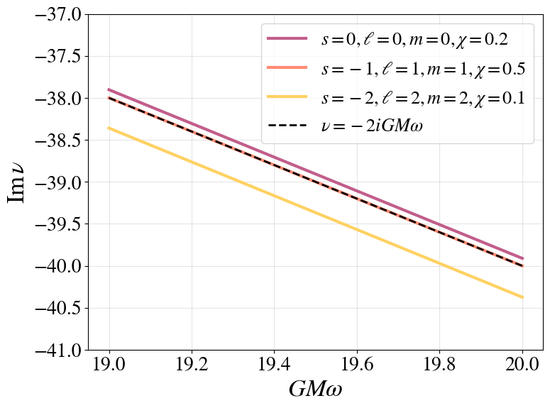
Figure 1: Numerical evaluation of the high frequency behavior of renormalized angular momentum $\nu$ using Black Hole Perturbation Toolkit BHP . The solid lines represent $\nu$ for various perturbation parameters. The dashed line is the analytic estimation from (18).

IV Generic-$\ell$ vs fixed-$\ell$ prescriptions

Physical angular momentum $\ell$ attain positive integers values with $\ell\geq|s|$. However, when we fix $\ell=n\in\mathbb{N}$, from (7) we observe $a$ becomes a half-integer at leading order in $\epsilon$. This complicates the structure of the PM expansion, since we are expanding close to the poles of the NS-function and of the gamma functions in (9). Considering for example the case $n=0$ ($s=\ell=m=0$), $a\simeq-1/2$, the leading divergence in terms of $a$ in the NS-function can be written as Gorsky et al. (2018)

$$F\sim\sum_{k=1}^{\infty}\frac{(m_{1}m_{2}m_{3}L)^{k}}{(2a+1)^{2k-1}}=\mathcal{O}(\epsilon^{2})\,.$$ (19)

Substituting the Kerr dictionary (5), we see no $1/\epsilon$ singularities actually appear in $F$ since the residue of the $2a=-1$ pole cancels such divergences. However, it is crucial to notice that all terms with $k\geq 1$ in the $L$ series in (19) will contribute to the $\epsilon^{2}$ order. In this sense, the naive $L$-expansion no longer coincide with the PM expansion, and a resummation is needed. A similar argument can be made for the divergent gamma factors entering in (9), and for any $s,\ell,m$. Note that these complications appear when one hits the poles of the NS-function, that is, after $\mathcal{O}(\epsilon^{2\ell+1})$: no integer-$\ell$ issue will arise before the horizon effects start to become important.

To avoid this kind of difficulties, we instead follow the route of analytically continue from $\ell\in\mathbb{N}$ to $\ell\in\mathbb{C}$, performing the low-frequency expansion in $L\sim\epsilon\ll 1$ and going back to the physical limit $\ell\in\mathbb{N}$ only at the final stage of the computations: we dub this approach the generic-$\ell$ prescription Kol and Smolkin (2012).

We use the generic-$\ell$ prescription at the level of the phase-shift (3). Let us then comment on the structure of ${}_{s}\delta_{\ell m}^{P}$ in this approach. For starters, even though $\tilde{F}$ is purely real, $\partial_{m_{3}}\tilde{F}$ in (8) breaks the symmetries of the invariants combinations listed in (11), and therefore it contains both real and imaginary parts. It is desirable to separate the real and imaginary contributions to ${}_{s}\delta_{\ell m}^{P}$ as they are associated to conservative and dissipative effects respectively. Interestingly, based on the conservation of energy flux between infinity and the horizon, the identity (see Eq.(68) in Ref. Mano and Takasugi (1997))

$$e^{{\rm Re}[\partial_{m_{3}}F]}\Bigg{|}\frac{\Gamma\left(\frac{1}{2}-a-m_{3}\right)}{\Gamma\left(\frac{1}{2}-a+m_{3}\right)}\Bigg{|}=|A_{s}^{P}|^{-1}~{},s<0~{},a\in\mathbb{R}~{}.$$ (20)

combined with Eq. (3), allows to conclude that in the low-frequency limit, the far zone scattering is purely elastic whereas only the near zone contributes to the absorption probability $\Gamma\sim\sum_{P}[1-({}_{s}\eta_{\ell m}^{P})^{2}$] Saketh et al. (2022, 2023). Indeed, by combining (20) with Eq. (8) and Eq. (3), one can straightforwardly get the far and near contributions to the phase-shift

$$\begin{split}{}_{s}\delta_{\ell m}^{P,\rm FZ}&=\underbrace{\frac{1}{2}{\rm Im}\left[\partial_{m_{3}}F\right]{-}\frac{1-\kappa}{2}\epsilon+\frac{1}{2}{\rm Arg}[A_{s}]}_{\rm rational}{+}\underbrace{\epsilon\log(2|\epsilon|)}_{\rm tail}\\ &+\underbrace{\frac{1}{2}{\rm Arg}\left[\frac{\Gamma(\frac{1}{2}{-}a{-}m_{3})}{\Gamma(\frac{1}{2}{-}a{+}m_{3})}\right]{+}\frac{\pi}{2}\left(\ell{+}\frac{1}{2}{+}a\right)}_{\rm transcendental}~{},\end{split}$$ (21)

$${}_{s}\delta_{\ell m}^{P,\rm NZ}=\frac{1}{2}{\rm Arg}\left[\frac{1+e^{-i\pi a}\mathcal{K}}{1+e^{i\pi\alpha}\frac{\cos(\pi(m_{3}-a))}{\cos(\pi(m_{3}+a))}\mathcal{K}}\right]~{},$$ (22)

and

$${}_{s}\eta_{\ell m}^{P}=\Bigg{|}\frac{1+e^{-i\pi a}\mathcal{K}}{1+e^{i\pi\alpha}\frac{\cos(\pi(m_{3}-a))}{\cos(\pi(m_{3}+a))}\mathcal{K}}\Bigg{|}~{}.$$ (23)

In Eq. (21), we also observe that the NS-function $F$ only contributes to the rational function of $\ell$ while the transendental contributions come from the ratio of gamma function and the additional $\pi$ factor. The logarithmic tail terms represent the imprints from the long-range Newtonian potential.

The drawback of the generic $\ell$ prescription is that when taking the physical limit $\ell\rightarrow\mathbb{N}$ at a given order in $\epsilon$, we encounter spurious poles at $\ell\in\mathbb{N}$ Casals and Ottewill (2015); Casals et al. (2016) both in the near and far zones . Consider for instance the $s=0$ perturbation at order $\epsilon^{4}$ ; its exhibits the specific pole structure:

$${}_{0}\delta_{\ell 1}^{\rm FZ}|_{\ell\rightarrow 1} =\frac{\chi}{72(\ell-1)}\epsilon^{4}+{\rm const}~{},$$ (24)

$$\quad{}_{0}\delta_{\ell 1}^{\rm NZ}|_{\ell\rightarrow 1} =-\frac{\chi}{72(\ell-1)}\epsilon^{4}+{\rm const}~{}.$$

To avoid these poles, the traditional MST approach uses a fixed-$\ell$ prescription, i.e. fixing $\ell,m\in\mathbb{N}$ before solving the Teukolsky equation Casals and Ottewill (2015); Casals et al. (2016). Intriguingly, as Eq. (24) demonstrates, the poles in the near-zone precisely cancels those in the far zone, a pattern we have verified up to the $\mathcal{O}(\epsilon^{8})$, for generic $s,\ell,m$. This cancellation suggests that the poles encountered when $\ell\rightarrow\mathbb{N}$ are essentially unphysical, and thus should cancel in any physical interpretation. A similar cancellation in an example of connection formula for hypergeometric function was pointed out in Ref. Kol and Smolkin (2012). For illustrative purposes, in Appendix A we include a explicit example keeping the non-divergent terms contributing in (24). Moreover, a detailed comparison of the constant piece shows that when adding near-zone and far zone together, the results obtained using the generic- and fixed-$\ell$ prescriptions completely agree with each other; we thus propose,

$$\left({}_{s}\delta_{\ell m}^{P,\rm FZ}+{}_{s}\delta_{\ell m}^{P,\rm NZ}\right)\Big{|}_{\ell\rightarrow\mathbb{N}}={}_{s}\delta_{(\ell\in\mathbb{N})m}^{P,\rm FZ}+{}_{s}\delta_{(\ell\in\mathbb{N})m}^{P,\rm NZ}~{},$$ (25)

indicating that the two limit $\ell\rightarrow\mathbb{N},\epsilon\rightarrow 0$ actually commute. In the remaining of this paper we only use the generic-$\ell$ formulation. We also stress here that the near-far factorization is only well-defined in the generic $\ell$ prescription. In the fixed-$\ell$ prescription, it is ill-defined and applying it leads to the effect of propagating non-Kerr particles in the $s-$ and $u-$ channels of the Compton amplitude, as observed in Eq. $(4.19)$ in Bautista et al. (2022). This is because for $\ell\in\mathbb{N}$ when expanded in $\epsilon$, the two contributions $\sigma=\pm 1$ in (4) mix with each other, i.e. $L^{a}$ and $L^{-a}$ both scale has half-integer scaling power, and hence one cannot separate the far-zone, $\sigma=-1$ piece from that.

The generic $\ell$ prescription also makes manifest of the locality structure of the scattering potential. This can be seen by fixing $\omega$ such that $\epsilon<1$ and taking $\ell\rightarrow\infty$, where the near zone and far zone phase-shift take following form respectively

$${}_{s}\delta_{\ell m}^{\rm FZ}\sim\epsilon\log(\epsilon\ell)+\sum_{n=1}^{\infty}\frac{\epsilon^{n+1}}{\ell^{n}}~{},\quad{}_{s}\delta_{\ell m}^{\rm NZ}\sim\epsilon^{2\ell+1}\sim(r_{s}\omega)^{2\ell+1}~{}.$$ (26)

In this regime, except for the logarithmic dependence $\log(\ell)$, the far zone shows the power law decay while the near zone features an exponential decay when $\ell\rightarrow\infty$. Physically, the logarithmic term reveals the long-range nature of the Newtonian $GM/r$ potential. The power law behavior $1/\ell^{n}$ indicates that all the PM-corrections share the non-local power law decay in the potential $(GM/r)^{n},n\geq 2,n\in\mathbb{N}$ when the radius $r\rightarrow\infty$. The near zone phase-shift reveals the common feature for the scattering against a localized potential, i.e. potentials with exponential decay also known as “hard-sphere” scattering Landau and Lifshits (1991), where the low-energy scattering at large $\ell$ shares the universal behavior $(\omega R)^{2\ell+1}$, with $R$ the range of the potential.

V Far-zone, tree-level gravitational Compton Amplitude for Kerr

In this section we analyze the point-particle limit of massless perturbations of the KBH in the context of the tree-level, helicity preserving, Gravitational Compton amplitude. As discussed above, this limit can be studied completely from the far zone contributions to the phase-shift (21) while ignoring the near zone tidal effects capture by (22). We recall we use the generic-$\ell$ prescription.

Consider then a $s=-2$ PW scattering off KBH. The wave impinges with momentum $k_{2}^{\mu}$ and scatters with momentum $k_{3}^{\mu}$, over the BH with momentum $p_{1}^{\mu}=Mu^{\mu}$. The angle formed by the direction of the impinging wave and the BH’s spin, $a_{\text{BH}}^{\mu}$, is $\gamma$. The far zone, helicity preserving amplitude is computed from the infinite sum of harmonics Dolan (2008)

$$\mathcal{A}{=}\sum_{\ell,m}\left[{}_{-2}S_{\ell m}\left(\gamma,0;\frac{\epsilon\chi}{2}\right){}_{-2}S_{\ell m}\left(\vartheta,\varphi;\frac{\epsilon\chi}{2}\right)\mathcal{A}_{\ell,m}\right]\,,$$ (27)

where

$$\mathcal{A}_{\ell m}=\frac{2\pi}{i\omega}\sum_{P=\pm 1}\left(e^{{}_{-2}\delta^{P,\text{FZ}}_{\ell m}(2i)}-1\right)\,.$$ (28)

The sum over $P$ is due to the change from the parity to helicity basis. As mentioned, we are interested in the contribution to the phase-shift of the form $\chi^{i}\epsilon^{i+1}\sim GM\omega(a_{\text{BH}}\omega)^{i}$; which exhibit explicitly a tree-level scaling. From the analysis based on the properties of the NS-function presented above, we know that ${}_{-2}\delta^{P,\text{FZ}}_{\ell m}$ not only captures purely conservative effects, but it is merely a polynomial function in $\chi$, making straightforward to extract its tree-level contributions to the amplitude. In fact, because of this polynomiality, these contributions are exact for Kerr in the sense that no analytic continuation in $\chi\gg 1$ is required.

Since we are using the generic$-\ell$ prescription, at this point one might worry that the $\ell$-poles discussed around eq. (24) will be problematic since we are dropping the near zone contributions responsible to cancel them. Fortunately, this poles do not contribute to the tree-level amplitude and can be safely ignored . In addition, since the $\epsilon$-corrections in $a$ are of the form $\sum_{i}c_{i}\chi^{i}\epsilon^{i+(n\geq 2)}$, we can simply use the tree-level value $a=-\frac{1}{2}-\ell$; this in turn provides a great simplification in the computation of ${}_{-2}\delta^{P,\text{FZ}}_{\ell m}$.

At leading order in the PM-expansion, we can arrange the amplitude modes (28) as

$$\mathcal{A}_{\ell m}{=}4\pi GMe^{i\Phi}\left(\psi^{(0)}(\ell{-}1)+\psi^{(0)}(\ell{+}3){+}\sum_{i=1}\beta_{\ell m}^{(i)}(\chi\epsilon)^{i}\right)\,,$$ (29)

where $\Phi=2\epsilon\log(2\epsilon)-\epsilon\to 0$, and we have written the explicit tree-level combinations $(\chi\epsilon)^{i}$, allowing for the $\beta$-coefficients to be functions only of $\ell$ and $m$. These coefficients are real, which makes manifest the conservative character of (29). We include the $\beta_{\ell m}^{(i)}$ coefficients needed to compute the tree-level far zone amplitude modes (29), up to $\mathcal{O}(a_{\text{BH}}^{8})$ in the ancillary files associated to the arXiv submission of this work anc .

Following Bautista et al. (2021, 2022), we match amplitude (27) together with (29), to a covariant tree-level classical ansatz of the form

$$\mathcal{A}=\mathcal{A}^{(0)}\left(e^{w-x}+f_{\xi}^{\text{FZ}}(x,y,w)\right)\,,$$ (30)

where $\mathcal{A}^{(0)}$ is the tree-level gravitational Compton amplitude for Schwarzschild BH and $\xi=(u\cdot(k_{2}+k_{3}))^{2}/(k_{3}-k_{2})^{2}$, is the scattering optical parameter. The contact term function, $f_{\xi}^{\text{FZ}}(x,y,w)$, is chosen in such way, the spurious pole in $w^{\geq 5}$, from expanding the exponential function in (30), is canceled. Here we have used the conventions of Cangemi et al. (2023) to write the spin operators: $x=(k_{3}{+}k_{2}){\cdot}a_{\text{BH}},\,y=(k_{3}{-}k_{2}){\cdot}a_{\text{BH}},\,w=\frac{2u\cdot k_{2}}{u\cdot\epsilon_{2}}\epsilon_{2}{\cdot}a_{\text{BH}}$, and the gauge $\epsilon_{2}^{\mu}=\frac{\langle 2|\sigma^{\mu}|3]}{\sqrt{2}[32]}\propto\tilde{\epsilon}_{3}^{\mu}=\frac{\langle 2|\sigma^{\mu}|3]}{\sqrt{2}\langle 32\rangle}\,$, with $|i\rangle,|i]$ the spinors of the massless momentum $k_{i}$.

After uniquely matching the modes of (29) to those obtained from (30), we finally obtain the contact terms $f_{\xi}^{\text{FZ}}(x,y,w)$, entering (30) to be:

$$\begin{split}f_{\xi}^{\text{FZ}}(x,y,w)=&\frac{1}{8!\times 9}\left[-128\left(w^{7}(2w+3x-6)\right)\xi^{-2}+64\upsilon_{1}w^{5}\xi^{-1}-8\upsilon_{2}w^{3}(w-x-y)(w-x+y)\right.\\ &\left.\qquad-4\upsilon_{3}w\left((w-x)^{2}-y^{2}\right)^{2}\xi-\upsilon_{4}\left((w-x)^{2}-y^{2}\right)^{3}\xi^{2}-278\left((w-x)^{2}-y^{2}\right)^{4}\xi^{3}\right]+\mathcal{O}(a_{\text{BH}}^{9})\,,\end{split}$$ (31)

where

$$\upsilon_{1}= -59w^{3}+3w^{2}(72-43x)+w\left(5x(60-23x)+y^{2}-504\right)+3x\left(x(68-19x)+y^{2}-168\right)-6y^{2}+756\,,$$ (32)

$$\upsilon_{2}= \,1199w^{3}{+}33w^{2}(77x{-}114){+}3w(2520{+}x(631x{-}1668){+}23y^{2}){+}3x(1680{-}638x{+}169x^{2}){+}33(x{-}2)y^{2}{-}7560\,,$$ (33)

$$\upsilon_{3}= \,2285w^{3}{+}w^{2}(3871x{-}5484){+}w\left(x(1949x{-}5172){+}97y^{2}{+}7560\right){+}9\left(x\left(x(27x{-}104){+}3y^{2}{+}280\right){-}6\left(y^{2}{+}70\right)\right)\,,$$ (34)

$$\upsilon_{4}= \,\,3355w^{2}+6w(581x-804)+x(659x-1752)+37y^{2}+2520\,.$$ (35)

Up to $\mathcal{O}(a_{\text{BH}}^{6})$, amplitude (31) agrees with the results reported in Table 1 in Bautista et al. (2022) for $\alpha=1$ and $\eta=0$, computed from the MST-method using the fixed-$\ell$ prescription. As expected, the far zone amplitude is independent of horizon effects and the boundary conditions used at $r_{+}$. Notice then that while in the fixed-$\ell$ prescriptions used in Bautista et al. (2022), the super extremal (SE) limit, $\chi\gg 1$, was needed to disentangle near from far physics effects, in the generic-$\ell$ prescription this continuation is not needed. In fact, as one can show, using the latter prescription, and after removing dissipative contributions, the dropped near-zone pieces vanish in the SE-limit (see Appendix A for a specific example). In addition, terms tagged with $\alpha$ in the results reported in Bautista et al. (2022) were interpreted as contributions coming from digamma functions in the SE-limit. Their appearance in the point-particle amplitude is just an artefact of using the fixed-$\ell$ prescription for computing the total phase-shift, which mixes the near and far zone effects, as explained above. From the discussion here, we conclude then no polygamma contributions actually appear in the point-particle Compton amplitude.

VI Discussion

In this work we have shown a new perspective on BHPT computations based on the use of NS-functions which makes manifest analytic properties and symmetries otherwise obscured by using other methods. It is desirable to further study the NS-function aiming to provide additional non-perturbative analytic results in classical physics.

Along these lines, in this work we have shown a natural separation between near and far zone physics, based on a generic-$\ell$ prescription. As it is well known Glampedakis and Andersson (2001); Bautista et al. (2021), this prescription is powerful for estimating the eikonal limit – $\ell\rightarrow\infty,\omega\rightarrow\infty$ while $\omega/\ell$ is fixed – of the classical observables. In this limit, results are universal –independent of the spin-weight $s$ of the perturbation – and receive contributions purely from far zone-physics. Studying the NS-function in this limit and its connection to geodesic motion is left for future work.

It is interesting to note also how the near-far factorization provides a natural separation of the spectrum of the theory. As it is well know, it can be access through the poles of the scattering amplitude. From (8), we thus identify two distinct types of poles in the Compton amplitudes. Firstly, in the eikonal limit – which only involves the far zone contributions – the poles appearing in $\Gamma\big{(}\frac{1}{2}-a-m_{3}\big{)}$ correspond to be the bound state energy associated with null geodesic motion; at leading order in $\epsilon$, they reduce to the bound states of the Newtonian potential, where the poles are located at $\epsilon=i\,,2i\,,3i\,,\cdots$ Bautista et al. (2021). The second type of poles come from near zone physics; they correspond to the quasi normal mode (QNM) resonances, for which the exact quantization condition follows as Aminov et al. (2022); Bonelli et al. (2022)

$$1+e^{i\pi a}\frac{\cos(\pi(m_{3}-a))}{\cos(\pi(m_{3}+a))}\mathcal{K}=0~{}.$$ (36)

This relation establishes a direct link between the tidal response function $\mathcal{K}$ and the QNM spectrum. Interestingly, we also find that $\mathcal{K}$ can be written in terms of the full (instanton plus one-loop) NS free energy $F_{\rm full}$ Aminov et al. (2022); Bonelli et al. (2022)

$$e^{i\pi a}\frac{\cos(\pi(m_{3}-a))}{\cos(\pi(m_{3}+a))}\mathcal{K}=-e^{\partial_{a}F_{\rm full}}~{},$$ (37)

which could lead to some hidden structures to be further investigated. Additional methods based on the Thermodynamic Bethe Ansatz have been used to study applications of NS functions to QNMs Fioravanti and Gregori (2021); Fioravanti et al. (2022) and it would be interesting to study them in the context of scattering amplitudes.

Away from the point particle limit, Compton amplitudes receive contributions from the near-zone phase-shift (22) starting at order $\epsilon^{2\ell+1}$ – the order at which the BH horizon effects become important. – Intriguing, at this order the phase-shift comes with special polygamma functions of the form $\psi^{(n)}(i\frac{m\chi}{\kappa}{\pm}\ell)$. Inspection of near-zone phase-shift (22) suggests that when $\chi\leq 1$ the near-zone piece does not provide any tree-level information (see also Appendix A for a explicit example). There is however a subtlety with this observation since from the identity

$$\psi^{(n)}(z{\pm}\ell){=}\psi^{(n)}(z)\pm\sum_{k{=}0{+}\eta_{\pm}}^{\ell{-}1{+}\eta_{\pm}}\frac{({-}1)^{n}n!}{(z\pm k)^{n+1}}\,,$$ (38)

for $n,\ell\in\mathbb{Z}^{+}$ and $(\eta_{+},\eta_{-})=(0,1)$, polynomial contribution with tree-level scaling arise from (22), by means of the sum term in (38). It is therefore ambiguous to extract tree-level contributions from the near-zone phase-shift without invoking an analytic continuation in the Kerr spin parameter, since the association of polygamma contributions to loop effects can be done either before or after identity (38) has been used. Interestingly, since the additional tree-level contributions arising from the sum term in (38) can appear only once the square-root from $\kappa=\sqrt{1-\chi^{2}}$ is removed, i.e. from $\kappa^{2n}$ terms, and since $\kappa$ inside the polygamma functions always comes accompanied by a factor of $i$ (see also (5)), then tree-level scaling implies that factors involving $(i\kappa)^{2n}$ are purely real, signaling absorptive effects in a 4-point amplitude can never come in tree-level form. In an on-shell language, matching of absorptive effects to effective tree-level-like three-point has been consider recently Aoude and Ochirov (2023); Jones and Ruf (2023); Chen et al. (2023). The inclusion/interpretation of near-zone effects, their interplay with the constraints from dynamical multipole-moment on the Gravitational Compton amplitude recently proposed in Scheopner and Vines (2023) and the translations of the constrains imposed by the symmetry of the NS-function to the Compton amplitudes written in the covariant basis are left for future investigation.

Finally, the technology used here in the context of linear perturbation theory can be naturally imported to the study of non-linear perturbations of KBHs, since, the second order Teukolsky equations are still of confluent Heun-type but with the addition of nonlinear source, obtained from the first order solution Loutrel et al. (2021); Ripley et al. (2021). A comprehensive analysis utilizing this novel method and their interplay with second order self force approaches are left future investigation.

Acknowledgments. We would like to thank Paolo Arnaudo, Alba Grassi, Aidan Herderschee, Misha Ivanov, Henrik Johansson, Chris Kavanagh, Yue-Zhou Li, Francisco Morales, Julio Parra-Martinez, Giorgio Di Russo and Justin Vines for useful discussions and comments on an early draft of this paper. We specially thank Chris Kavanagh for sharing his fixed-$\ell$ MST results for SE-Kerr Compton amplitude up to order $a_{\text{BH}}^{7}$, which are in complete agreement with (31) up to this order. This work makes use of the Black Hole Perturbation Toolkit BHP . The work of Y.F.B. has been supported by the European Research Council under Advanced Investigator Grant ERC–AdG–885414. The work of C.I. is partially supported by the Swiss National Science Foundation Grant No. 185723. The research of G.B. is partly supported by the INFN Iniziativa Specifica ST&FI and by the PRIN project “Non-perturbative Aspects Of Gauge Theories And Strings”. The research of A.T. is partly supported by the INFN Iniziativa Specifica GAST and InDAM GNFM. The research of G.B and A.T. is partly supported by the MIUR PRIN Grant 2020KR4KN2 ”String Theory as a bridge between Gauge Theories and Quantum Gravity”. G.B. and A.T. acknowledge funding from the EU project Caligola HORIZON-MSCA-2021-SE-01), Project ID: 101086123.

Appendix A Appendix A: MST Method Review and Near-Far Factorization

We start this appendix by reviewing the MST method  Mano et al. (1996a, b); Mano and Takasugi (1997); Sasaki and Tagoshi (2003) for solving TME using matching asymptotic expansion, where the renormalized angular momentum $\nu$ is introduced. As a consequence of the matching asymptotic expansion, we then discuss the near-far factorization in the Compton scattering phase-shift ${}_{s}\delta_{\ell m}$. Finally, we explicitly show that in the generic $\ell$ prescription, there are spurious poles in the MST coefficients when $\ell\in\mathbb{N}$ and it will be cancelled when adding near-zone and far zone

A.1 MST Method Review

In the MST approach, one first constructs the near-zone solution based on a double-sided infinite series of hypergeometric functions which converges within $r_{+}\leq|r|<\infty$ . This convergence radius gives a natural definition for the near-zone:

$$\textbf{MST Near Zone}:r_{+}\leq|r|<\infty~{}.$$ (39)

Similarly, one then constructs the far zone solution based a double-sided infinite series of Coulomb wavefunction which converges within $r_{+}<|r|\leq\infty$, which can be used as the definition of far zone:

$$\textbf{MST Far Zone}:r_{+}<|r|\leq\infty~{}.$$ (40)

To get the solution that is converging everywhere, one needs to match the near-zone solution with far-zone solution in the overlapping region $r_{+}<r<\infty$. In fig. 2, we show a schematic diagram for the matching asymptotic expansion.

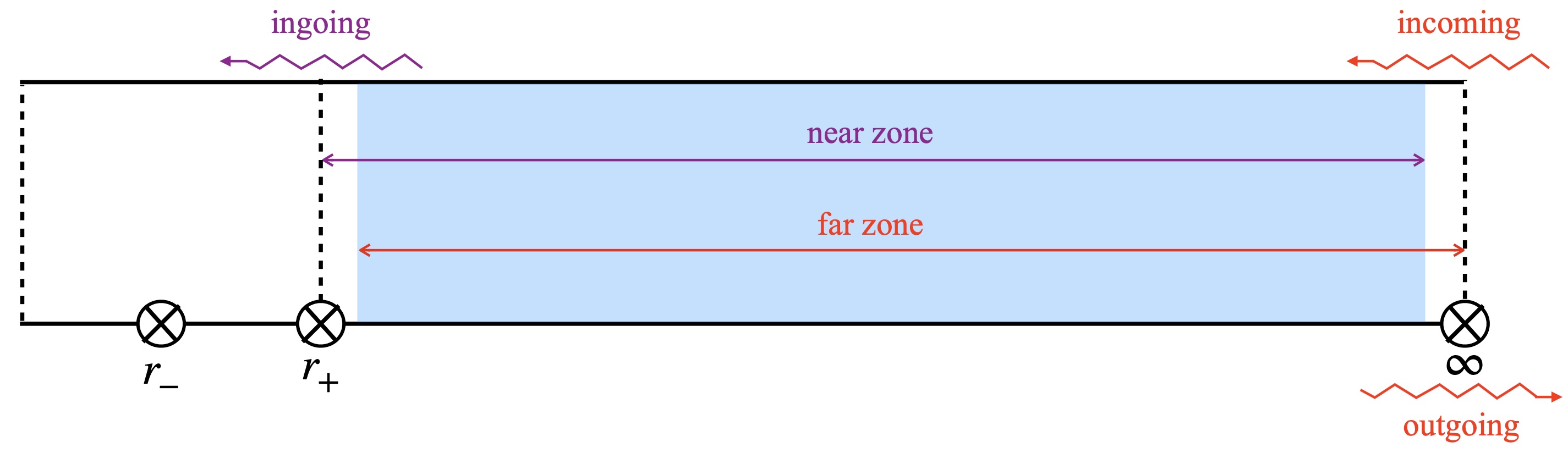
Figure 2: A schematic diagram illustrates the convergence radius of near and far zone solutions. The blue region denotes the overlapping region where the matching is performed.

To ensure the convergence and the matching of the solutions on both sides, one needs to introduce an auxiliary non-integer parameter, the so-called renormalized angular momentum $\nu(s,\ell,m,\omega)$, which is a function of spin-weight $s$, angular momentum $\ell$, azimuthal quantum number $m$, and the frequency $\omega$ of the perturbation. In the low-frequency region it has the form

$$\nu=\ell+\frac{1}{2\ell+1}\left(-2-\frac{s^{2}}{\ell(\ell+1)}+\frac{\left[(\ell+1)^{2}-s^{2}\right]^{2}}{(2\ell+1)(2\ell+2)(2\ell+3)}-\frac{\left(\ell^{2}-s^{2}\right)^{2}}{(2\ell-1)2\ell(2\ell+1)}\right)\epsilon^{2}+\mathcal{O}\left(\epsilon^{3}\right)~{},$$ (41)

where $\epsilon\equiv 2GM\omega$. Formally, $\nu$ is known as the characteristic exponent because it governs the following asymptotic behavior of the near-zone ingoing solution (see Eq. (166) in Sasaki and Tagoshi (2003))

$${}_{s}R_{\ell m}^{\rm near}\sim K_{\nu}r^{\nu}+K_{-\nu-1}r^{-\nu-1}~{},\quad r\rightarrow\infty~{}.$$ (42)

The coefficient ratio $K_{-\nu-1}/K_{\nu}$ tells the relative amplitude between the decaying $r^{-\nu-1}$ and the growing $r^{\nu}$ mode which captures the BH tidal response. As mentioned in the main text, a detailed comparison between CFT method and MST method shows that $\mathcal{K}$ given in (8) agrees with $K_{-\nu-1}/K_{\nu}$ and thus we call $\mathcal{K}$ the BH tidal response function. After performing the matching, and imposing the appropriate boundary conditions (2), one finally obtains the wave amplitude ratio as follows:

$$\frac{B_{s\ell m}^{\text{refl}}}{B_{s\ell m}^{\text{inc}}}{=}\frac{1}{\omega^{2s}}{{\color[rgb]{0.12109375,0.46484375,0.70703125}\underbrace{\frac{1+ie^{i\pi\nu}\frac{K_{-\nu-1;s}}{K_{\nu;s}}}{1{-}ie^{-i\pi\nu}\frac{\sin(\pi(\nu{-}s{+}i\epsilon))}{\sin(\pi(\nu+s-i\epsilon))}\frac{K_{{-}\nu{-}1;s}}{K_{\nu;s}}}}_{\text{near\,zone}}}}{{\color[rgb]{0.83984375,0.15234375,0.15625}\underbrace{\times\frac{A_{-;s}^{\nu}}{A_{+;s}^{\nu}}e^{i\epsilon(2\ln\epsilon-(1-\kappa))}}_{\text{far\,zone}}}}\,,$$ (43)

where

$$\frac{A_{-;s}^{\nu}}{A_{+;s}^{\nu}}=\frac{e^{-{\pi}i(\nu+1)}}{2^{2(s-i\epsilon)}}\times\frac{\Gamma(\nu+1+s-i\epsilon)}{\Gamma(\nu+1-s+i\epsilon)}\times\frac{\sum_{n=-\infty}^{+\infty}(-1)^{n}{(\nu+1+s-i\epsilon)_{n}\over(\nu+1-s+i\epsilon)_{n}}a_{n}^{\nu}}{\sum_{n=-\infty}^{+\infty}a_{n}^{\nu}}\,,$$ (44)

and

$$\frac{K_{-\nu-1;s}}{K_{\nu;s}}=(2\epsilon\kappa)^{2\nu+1}\frac{\Gamma(-2\nu-1)\Gamma(-2\nu)\Gamma(\nu-i\tau+1)\Gamma(-s-i\epsilon+\nu+1)\Gamma(-s+i\epsilon+\nu+1)}{\Gamma(2\nu+1)\Gamma(2\nu+2)\Gamma(-\nu-i\tau)\Gamma(-s-i\epsilon-\nu)\Gamma(-s+i\epsilon-\nu)}\times\frac{X_{-\nu-1}}{X_{\nu}}~{}.$$ (45)

Here, $\kappa=\sqrt{1-\chi^{2}}$ and $\tau=(\epsilon-m\chi)/\kappa$. The function $X_{\nu}$ is given by the product of two infinity sum of the MST coefficients, $a_{n},-\infty\leq n\leq+\infty$;

$$X_{\nu} =\left(\sum_{n=0}^{+\infty}\frac{(-1)^{n}}{n!}(1+2\nu)_{n}a_{n}^{\nu}\frac{(1+\nu+s+i\epsilon)_{n}}{(1+\nu-s-i\epsilon)_{n}}\frac{(1+\nu+i\tau)_{n}}{(1+\nu-i\tau)_{n}}\right)\times\left(\sum_{n=-\infty}^{0}\frac{(-1)^{n}}{(-n)!(2\nu+2)_{n}}\frac{(\nu+1+s-i\epsilon)_{n}}{(\nu+1-s+i\epsilon)_{n}}a_{n}^{\nu}\right)^{-1}\,~{}.$$ (46)

MST coefficients satisfy the following three term recurrence relation along with the “renormalized” angular momentum $\nu$

$$\alpha_{n}^{\nu}a_{n+1}^{\nu}+\beta_{n}^{\nu}a_{n}^{\nu}+\gamma_{n}^{\nu}a_{n-1}^{\nu}=0~{},$$ (47)

where

$$\alpha_{n}^{\nu} =\frac{i\epsilon\kappa(n+\nu+1+s+i\epsilon)(n+\nu+1+s-i\epsilon)(n+\nu+1+i\tau)}{(n+\nu+1)(2n+2\nu+3)}$$ (48)

$$\beta_{n}^{\nu} =-{}_{s}\lambda_{\ell}^{m}-s(s+1)+(n+\nu)(n+\nu+1)+\epsilon^{2}+\epsilon(\epsilon-m\chi)+\frac{\epsilon(\epsilon-m\chi)\left(s^{2}+\epsilon^{2}\right)}{(n+\nu)(n+\nu+1)}$$

$$\gamma_{n}^{\nu} =-\frac{i\epsilon\kappa(n+\nu-s+i\epsilon)(n+\nu-s-i\epsilon)(n+\nu-i\tau)}{(n+\nu)(2n+2\nu-1)}.$$

We fix $a_{0}=1$ for convenience. These recurrence relations can be solved order by order in the PM expansion.

Let us finally provide the explicit expressions for the Teukolsky-Starobinsky constant $A_{s}^{P}$ entering (3)

$$A_{0}^{\pm}=1\,,$$ (49)

$$A_{-1}^{\pm}=\left[\left({}_{-1}Q_{\ell m}+a^{2}\omega^{2}-2am\omega\right)^{2}+4am\omega-4a^{2}\omega^{2}\right]^{1/2}~{},$$

$$A_{-2}^{\pm}=\Bigg{[}\left(({}_{-2}Q_{\ell m})^{2}+4a\omega m-4a^{2}\omega^{2}\right)\left[({}_{-2}Q_{\ell m}-2)^{2}+36a\omega m-36a^{2}\omega^{2}\right]$$

$$\quad+(2{}_{-2}Q_{\ell m}-1)\left(96a^{2}\omega^{2}-48a\omega m\right)-144\omega^{2}a^{2}\Bigg{]}^{1/2}\pm i12M\omega~{},$$

where ${}_{s}Q_{\ell m}\equiv{}_{s}\lambda_{\ell m}+s(s+1)$. ${}_{s}\lambda_{\ell m}$ is the angular eigenvalue of the spheroidal harmonics.

A.2 Near-Far Factorization

The near-far factorization proposed in Ivanov and Zhou (2022); Saketh et al. (2023) shows that the Kerr Compton scattering phase shift once expanded in the small frequency limit, i.e. $GM\omega\ll 1$ can be directly separated into the near zone and far zone contributions. The far-zone phase shift has the following feature

$${}_{s}\delta_{\ell m}^{\rm FZ}\sim(GM\omega)\log(GM\omega)+(GM\omega)+(GM\omega)^{2}+(GM\omega)^{3}+\cdots$$ (50)

which features integer power of $G$ scaling except for the logarithmic term due to the scattering off long-range Newtonian potential. Higher order in $G$ corrections can be understood as the PM corrections upon the point-particle approximation. The near-zone phase shift features non-analytic behavior of $G$

$${}_{s}\delta_{\ell m}^{\rm NZ}\sim(GM\omega)^{2\nu+1}(1+(GM\omega)+(GM\omega)^{2}+\cdots)~{},$$ (51)

for generic value of $\nu$. Once performing the low-frequency expansion, the non-analyticity leads to the logarithmic corrections

$$\left.(GM\omega)^{2\nu+1}\right|_{\nu=\ell+\mathcal{O}\left((GM\omega)^{2}\right)+\ldots}=(GM\omega)^{2\ell+1}\left(1+(GM\omega)^{2}\log(GM\omega)+\cdots\right)~{},$$ (52)

which have a natural understanding in terms of the renormalization group (RG), where are running of “dynamical” Love numbers for Kerr BHs appears Saketh et al. (2023).

A.3 phase-shifts for $s=0,\ell=1,m=1$ Perturbations

For illustrative purposes, let us close this appendix by explicitly showing the cancellation of the $\ell$-poles at the level of the phase-shift in the scalar example presented in the main text. We keep up to $\mathcal{O}(\epsilon^{4})$, which for the $s=0,\ell=m=1$ case, is the order at which the first poles appear. In the generic-$\ell$ prescription, the near- and far- zone contributions take the form respectively

$$\begin{split}{}_{0}\delta_{\ell 1}^{\rm NZ}|_{\ell{\rightarrow}1}{=}&{\color[rgb]{0.12109375,0.46484375,0.70703125}\left(\frac{\chi}{72(\ell{-}1)}{+}\left(\frac{\gamma_{E}}{18}-\frac{7}{54}\right)\chi+\frac{1}{36}\chi\log(2\epsilon\kappa)+\frac{1}{36}\chi{\rm Re}\left[\psi^{(0)}\left(\frac{i\chi}{\kappa}-1\right)\right]\right)\epsilon^{4}}\end{split}$$ (53)

and

$$\begin{split}{}_{0}\delta_{\ell 1}^{\rm FZ}|_{\ell{\rightarrow}1}&={\color[rgb]{0.83984375,0.15234375,0.15625}\epsilon\log(2|\epsilon|)+\left(-\frac{3}{2}+\gamma_{E}\right)\epsilon+\left(\frac{19}{60}\pi-\frac{\chi}{4}\right)\epsilon^{2}+\left(\frac{19}{180}\pi^{2}-\frac{7\pi\chi}{60}+\frac{\chi^{2}}{40}-\frac{\zeta(3)}{3}\right)\epsilon^{3}}\\ &\quad+{\color[rgb]{0.83984375,0.15234375,0.15625}\left(-\frac{\chi}{72(\ell-1)}+\frac{78037}{378000}\pi-\frac{130+42\pi^{2}}{1080}\chi+\frac{143}{4200}\pi\chi^{2}+\frac{\chi^{3}}{40}\right)\epsilon^{4}}~{}.\end{split}$$ (54)

The same computation can be done in the fixed-$\ell$ prescription. Using the MST coefficients listed in Appendix B in Casals et al. (2016), we have

$$\begin{split}{}_{0}\delta_{11}=&{\color[rgb]{0.83984375,0.15234375,0.15625}\epsilon\log(2|\epsilon|)+\left({-}\frac{3}{2}{+}\gamma_{E}\right)\epsilon+\left(\frac{19\pi}{60}{-}\frac{13\chi}{57}\right)\epsilon^{2}+\left(\frac{19\pi^{2}}{180}{-}\frac{1583\chi^{2}}{137180}{-}\frac{9\pi\chi}{95}{-}\frac{\zeta(3)}{3}{-}\frac{5}{228}\right)\epsilon^{3}}\\ &{\color[rgb]{0.83984375,0.15234375,0.15625}+\left(\frac{8100833\chi^{3}}{831969264}{-}\frac{17947\pi\chi^{2}}{7201950}{-}\left(\frac{92867}{2880780}{+}\frac{3\pi^{2}}{95}\right)\chi{+}\frac{1325203\pi}{7182000}\right)\epsilon^{4}}\\ &{\color[rgb]{0.12109375,0.46484375,0.70703125}{-}\frac{5\chi\epsilon^{2}}{228}{+}\left(\frac{5}{228}{-}\frac{5\pi}{228}\chi+\frac{2005\chi^{2}}{54872}\right)\epsilon^{3}{+}\epsilon^{4}\left(\frac{5\pi}{228}+\frac{2005\pi}{54872}\chi^{2}+\frac{63491993}{4159846320}\chi^{3}\right.}\\ &{\color[rgb]{0.12109375,0.46484375,0.70703125}\left.+\chi\left(\frac{1}{36}{\rm Re}\left[\psi^{(0)}\left(\frac{i\chi}{\kappa}-1\right)\right]+\frac{1}{36}\log(2\kappa\epsilon)-\frac{5\pi^{2}}{684}-\frac{156832}{720195}+\frac{\gamma_{E}}{18}\right)\right)}\,.\end{split}$$ (55)

By combining (53) and (54), we find that the diverging terms $1/(\ell-1)$ cancel, aligning perfectly with the results shown in (55). The colors in the fixed-$\ell$ results denote a hypothetical near-far factorization. From (55), we see that with the fixed-$\ell$ prescription, there are no singular contributions in any region, but this comes at the cost of mixing the terms from the near and far zones. For instance, the tree-level contributions, i.e. terms scale as $\chi^{i}\epsilon^{i+1}$, entirely come from the far zone in generic-$\ell$ prescriptions

$${\color[rgb]{0.83984375,0.15234375,0.15625}\underbrace{-\frac{1}{40}\chi^{3}\epsilon^{4}+\frac{\chi^{2}\epsilon^{3}}{40}+\frac{\chi\epsilon^{2}}{4}}_{{\rm generic}-\ell\,{\rm far\,zone}}}={\color[rgb]{0.83984375,0.15234375,0.15625}\underbrace{-\frac{13\chi}{57}\epsilon^{2}-\frac{1583\chi^{2}}{137180}\epsilon^{3}+\frac{8100833\chi^{3}}{831969264}\epsilon^{4}}_{{\rm fixed}-\ell\,{\rm far\,zone}}}{\color[rgb]{0.12109375,0.46484375,0.70703125}\underbrace{-\frac{5\chi}{228}\epsilon^{2}+\frac{2005\chi^{2}}{54872}\epsilon^{3}+\frac{63491993\chi^{3}}{4159846320}\epsilon^{4}}_{{\rm fixed}-\ell\,{\rm near\,zone}}}~{},$$ (56)

while the fixed-$\ell$ prescription splits these terms into unusual and confusing mixes.

There is however a subtlety when extracting tree-level contributions as showed in the discussion section. From (53) no apparent tree-level contribution arises for $\chi\leq 1$, however if identity (38) was used, the tree-level, contribution $\chi^{3}\epsilon^{4}/36$ will be extracted from (53). To avoid this subtlety, and in order to extract tree-level contribution in the point particle limit, in Refs. Bautista et al. (2021, 2022) the super-extremal (SE) limit was necessary. However, because of the near-far zone mixing in the fixed-$\ell$ prescription used in those references, in combination of the use of identity (38), an apparent contribution from digamma function, tagged with the $\alpha$-label, appeared in the point-particle amplitude. The $\alpha$-label was added to the digamma appearing in the right-hand-side of (38). In the generic-$\ell$ prescription, this mix does not take place and, as one can explicitly check, no tree-level contribution arises from (53) in the SE-limit.

The resulting covariant tree-level amplitude computed with (56) agrees with the results in eq. (4.54-4.55) in Bautista et al. (2021). The extra $\chi^{3}\epsilon^{4}/36$ would change such results precisely canceling the contact terms modifying the Born amplitudes eq. (4.54-4.55) in Bautista et al. (2021).

It is also interesting to analyze the contribution from the dissipative pieces. The absorption probability $\Gamma\sim\sum_{P}[1-({}_{s}\eta_{\ell m}^{P})^{2}]$ can be estimated from

$$\begin{split}{}_{0}\eta_{11}^{P}{=}{\color[rgb]{0.12109375,0.46484375,0.70703125}1+\frac{\epsilon^{3}}{36}\chi+\frac{\epsilon^{4}}{36}\left[\Big{(}\pi{-}2\text{Im}\left[\psi^{(0)}\Big{(}\frac{i\chi}{\kappa}{-}1\Big{)}\right]\Big{)}\chi{-}(1{-}\kappa)\left(2\chi^{2}{+}1\right)\right]}~{}.\end{split}$$ (57)

Interestingly, even after using identity (38), no-tree level contribution arises from the imaginary part of the near-zone. This signals dissipative effects arise purely as loop-contributions.

As a final remark, notice that from (53), no real term of the form $\chi^{2}\epsilon^{3}$ arises in the near-zone phase-shift. This is indeed corresponds to the vanishing of the static leading Love number for $s=0$ perturbations off Kerr.

Appendix B Appendix B: CFT Method Review

In this appendix we briefly review the argument of Bonelli et al. (2023) to compute the CHE connection coefficients. Let us start by setting the notation: we consider Liouville CFT (for a review of Liouville theory, see Teschner (2001)), and parametrize the central charge as $c=1+6Q^{2}$, with $Q=b+b^{-1}$. We indicate primary operators of dimensions $\Delta_{i}=Q^{2}/4-\alpha_{i}^{2}$ as $V_{\alpha_{i}}(z_{i})$, and the corresponding primary states as $|\Delta_{i}\rangle$. $\alpha_{i}$ is usually referred to as the Liouville momentum. Crucial for our discussion will be the so called rank 1 irregular state $\langle\mu,\Lambda|$ Gaiotto (2013); Bonelli et al. (2012); Gaiotto and Teschner (2012), which is defined as the state such that

$$\langle\mu,\Lambda|L_{0}=\Lambda\partial_{\Lambda}\,,\quad\langle\mu,\Lambda|L_{-1}=\mu\Lambda\langle\mu,\Lambda|L_{-1}\,,\quad\langle\mu,\Lambda|L_{-2}=-\frac{\Lambda^{2}}{4}\langle\mu,\Lambda|L_{-2}\,.$$ (58)

B.1 Connection Formula for CHE

Let us consider the Liouville correlator

$$\langle\mu,\Lambda|V_{\alpha_{1}}(1)\Phi_{2,1}(z)|\Delta_{\alpha_{0}}\rangle\,,$$ (59)

where $\Phi_{2,1}$ is the level degenerate state of weight $\Delta_{2,1}=-\frac{1}{2}-\frac{3}{4}b^{2}$ that satisfies

$$\left(b^{-2}L_{-1}^{2}+L_{-2}\right)\Phi_{2,1}(z)=0\,.$$ (60)

Since Virasoro generators act as differential operators when inserted in correlation functions, equation (60) turns into a differential equation for the correlator (59), that is the Belavin–Polyakov–Zamolodchikov (BPZ) equation Belavin et al. (1984)

$$\left(b^{-2}\partial_{z}^{2}+\left(\frac{1}{z}+\frac{1}{z-1}\right)\partial_{z}+\frac{\Lambda\partial_{\Lambda}-\Delta_{2,1}-\Delta_{0}-\Delta_{1}}{z(z-1)}+\frac{\Delta_{0}}{z^{2}}+\frac{\Delta_{1}}{(z-1)^{2}}+\frac{\mu\Lambda}{z}-\frac{\Lambda^{2}}{4}\right)\langle\mu,\Lambda|V_{\alpha_{1}}(1)\Phi_{2,1}(z)|\Delta_{\alpha_{0}}\rangle=0\,.$$ (61)

This is a partial differential equation in $\Lambda$ and $z$. In the semi-classical limit $b\rightarrow 0,\alpha_{i},\mu,\Lambda\rightarrow\infty$ such that $a_{i}=b\alpha_{i},m_{3}=b\mu,L=b\Lambda$ are finite, conformal blocks of (59) behave as Zamolodchikov and Zamolodchikov (1996)

$$\mathfrak{F}\sim\Lambda^{\Delta}\exp\left(\frac{F(a_{1}+a_{0},a_{1}-a_{0},m_{3},a,L)}{b^{2}}+W(L;z)+\mathcal{O}\left(b^{-2}\right)\right)\,,$$ (62)

where $F$ is the so called classical conformal block and $\Delta=Q^{2}/4-\alpha^{2}$ ($a$ being the semiclassical momentum $\lim_{b\to 0}b\alpha$) is the scaling dimension of the intermediate operator exchanged in the operator product expansion (OPE). The AGT correspondence Alday et al. (2010) relates the classical Virasoro block $F(a_{0}+a_{1},a_{1}-a_{0},m_{3},a,L)$ to the instanton partition function of an $SU(2)$ $\mathcal{N}=2$ supersymmetric gauge theory with $N_{f}=3$ hypermultiplets of masses

$$m_{1}=a_{0}+a_{1}~{},\quad m_{2}=a_{1}-a_{0}~{},\quad m_{3}=m_{3}~{}.$$ (63)

in the NS phase of the $\Omega$ background. Besides its physical significance, the AGT correspondence gives a very convenient way of computing $F$ as we will see in the following.

Note that the $z-$dependence in (62) enters at a subleading order in $b$, as one can expect from the fact that as $b$ goes to zero $\Delta_{2,1}$ is subleading with respect to $\Delta_{i},\mu,\Lambda$. Crucially

$$\Lambda\partial_{\Lambda}\mathfrak{F}=b^{-2}\left(\frac{1}{4}-a^{2}+L\partial_{L}F(L)+\mathcal{O}\left(b^{0}\right)\right)\equiv b^{-2}\left(u+\mathcal{O}\left(b^{0}\right)\right)\,.$$ (64)

The $\Lambda-$derivative decouples, leaving a new parameters, $u$, at its place. $u\equiv\frac{1}{4}-a^{2}$ is usually called the accessory parameter in the mathematical literature. All in all, semi-classical conformal blocks defined as

$$\mathcal{F}=\lim_{b\to 0}\Lambda^{-\Delta}e^{-\frac{1}{b^{2}}F}\mathfrak{F}$$ (65)

satisfy the ODE

$$\left(\partial_{z}^{2}+\frac{u-\frac{1}{2}+a_{0}^{2}+a_{1}^{2}}{z(z-1)}+\frac{\frac{1}{4}-a_{1}^{2}}{(z-1)^{2}}+\frac{\frac{1}{4}-a_{0}^{2}}{z^{2}}+\frac{m_{3}L}{z}-\frac{L^{2}}{4}\right)\mathcal{F}(z)=0~{},$$ (66)

This ODE has two regular singularities at $z=0,1$ excited by the primary states, and an irregular singularity of rank 1 at $z=\infty$ generated by the irregular state: it is the CHE in its normal form.

The $z-$dependence of $\mathcal{F}(z)$ can be extracted by computing the OPE of the degenerate operator $\Phi_{2,1}(z)$ with the other insertions. When $\Phi_{2,1}(z)$ fuses e.g. with another primary one has

$$\Phi_{2,1}(z)V_{\alpha_{i}}(z_{i})\sim\sum_{\pm}(z-z_{i})^{\frac{1}{2}\pm a_{i}}\left(V_{\alpha_{i}\pm}(z_{i})+\mathcal{O}(z-z_{i})\right)\,.$$ (67)

Inserting (67) into (59) one can extract the $z$ dependence on the blocks for $z\sim z_{i}$. The $\pm$ signs corresponds for the two conformal dimensions exchanged by the OPE, and accounts for the two linearly independent local solutions of the ODE. More precisely, one finds around $z=1$

$$\mathcal{F}_{\pm}^{(1)}(1-z)=e^{\mp\frac{1}{2}\partial_{a_{1}}F}(1-z)^{\frac{1}{2}+\pm a_{1}}~{},$$ (68)

and around $z=\infty$

$$\mathcal{F}_{\pm}^{(\infty)}(1/z)=e^{\mp\frac{1}{2}\partial_{m_{3}}F}e^{\pm Lz/2}L^{-\frac{1}{2}\mp m_{3}}z^{\mp m_{3}}~{}.$$ (69)

The connection formula can be worked out by using crossing symmetries in the conformal correlators. We refer the reader to Bonelli et al. (2023) for more details, and just sketch the main idea here. Crossing symmetry relates between each other different OPE decomposition of the correlator (59). As mentioned above different OPE decompositions reconstruct local solution of the ODE centered close to different singular points. Schematically, crossing symmetry constraint take the following form:

$$\sum_{\pm}(\text{3 pt functions})\big{|}\mathfrak{F}^{(1)}_{\pm}(1-z)\big{|}^{2}=\sum_{\pm}(\text{3 pt functions})\big{|}\mathfrak{F}^{(\infty)}_{\pm}(z^{-1})\big{|}^{2}\,.$$ (70)

The 3 point functions of Liouville CFT are non-perturbatively known Dorn and Otto (1994); Zamolodchikov and Zamolodchikov (1996). One can then use (70) to express e.g. $\mathfrak{F}^{(1)}_{+}(1-z)$ as a linear combination of $\mathfrak{F}^{(\infty)}_{\pm}(z^{-1})$. Upon taking the semi-classical limit, this allows use to compute the connection coefficients of the CHE. For the relevance of this paper, we quote the formula

$$\mathcal{F}_{\theta}^{(1)}(1-z)=\sum_{\theta^{\prime}=\pm}\mathcal{M}(\theta,\theta^{\prime})\mathcal{F}_{\theta^{\prime}}^{(\infty)}(1/z)~{},\quad\theta=\pm~{}.$$ (71)

with the connection matrix

$$\mathcal{M}(\theta,\theta^{\prime})=\sum_{\sigma=\pm}L^{\sigma a}\frac{\Gamma(1-2\sigma a)\Gamma(-2\sigma a)\Gamma\left(1+2\theta a_{1}\right)}{\Gamma\left(\frac{1}{2}+\theta a_{1}-\sigma a+a_{0}\right)\Gamma\left(\frac{1}{2}+\theta a_{1}-\sigma a-a_{0}\right)\Gamma\left(\frac{1}{2}-\sigma a-\theta^{\prime}m_{3}\right)}e^{i\pi\left(\frac{1-\theta^{\prime}}{2}\right)\left(\frac{1}{2}-m_{3}-\sigma a\right)}e^{-\frac{\sigma}{2}\partial_{a}F}~{}.$$ (72)

B.2 Solving Radial TME

Now, we apply the CFT method to solving the radial TME satisfied by ${}_{s}R_{\ell m}(r)$ in (1). Performing the following changing of variables

$$\Psi(z)=\Delta^{\frac{s+1}{2}}(r){}_{s}R_{\ell m\omega}(r)\,,\quad z=\frac{r-r_{-}}{r_{+}-r_{-}}\,,$$ (73)

the TME takes the form (66), the in-going solution to radial TME at the horizon can be written as

$$\Psi^{\rm in}(z)={}_{s}C^{-}_{\ell m}e^{\frac{Lz}{2}}z^{-m_{3}}\left(1+\mathcal{O}(z^{-1)}\right)+{}_{s}C^{+}_{\ell m}e^{-\frac{Lz}{2}}z^{m_{3}}\left(1+\mathcal{O}(z^{-1)}\right)$$ (74)

where ${}_{s}C^{\pm}_{\ell m}$ are elements of the Heun connection matrix (72). Explicitly,

$${}_{s}C^{-}_{\ell m}=\sum_{\sigma=\pm}L^{-\frac{1}{2}-m_{3}+\sigma a}\frac{\Gamma\left(1-2\sigma a\right)\Gamma\left(-2\sigma a\right)\Gamma\left(1+2a_{1}\right)}{\Gamma\left(\frac{1}{2}+a_{1}-\sigma a+a_{0}\right)\Gamma\left(\frac{1}{2}+a_{1}-\sigma a-a_{0}\right)\Gamma\left(\frac{1}{2}-\sigma a-m_{3}\right)}e^{-\frac{\sigma}{2}\partial_{a}F-\frac{1}{2}\partial_{m_{3}}F}\,,$$ (75)

$${}_{s}C^{+}_{\ell m}=\sum_{\sigma=\pm}(-L)^{-\frac{1}{2}+m_{3}+\sigma a}\frac{\Gamma\left(1-2\sigma a\right)\Gamma\left(-2\sigma a\right)\Gamma\left(1+2a_{1}\right)}{\Gamma\left(\frac{1}{2}+a_{1}-\sigma a+a_{0}\right)\Gamma\left(\frac{1}{2}+a_{1}-\sigma a-a_{0}\right)\Gamma\left(\frac{1}{2}-\sigma a+m_{3}\right)}e^{-\frac{\sigma}{2}\partial_{a}F+\frac{1}{2}\partial_{m_{3}}F}\,.$$

Mapping (74) to the asymptotic behavior given in (2), we get (8) in the main text.

B.3 Computation of $F$ and Symmetry Properties

As shown in (62), $F$ controls the $z-$independent part of the correlator (59), that is

$$\langle\mu,\Lambda|V_{\alpha_{1}}(1)|\Delta_{0}\rangle\,.$$ (76)

Small-$\Lambda$ conformal blocks of (76) are given by

$$\mathfrak{F}\left(\mu,\alpha_{i},\alpha,\Lambda\right)=\Lambda^{\Delta}e^{\left(\frac{Q}{2}+\alpha_{1}\right)\Lambda}\sum_{\vec{Y}}\Lambda^{|\vec{Y}|}z_{\text{vec}}\left(\vec{\alpha},\vec{Y}\right)z_{\text{hyp}}\left(\vec{\alpha},\vec{Y},-\mu\right)\prod_{\theta=\pm}z_{\text{hyp}}\left(\vec{\alpha},\vec{Y},\alpha_{1}+\theta\alpha_{0}\right)\,.$$ (77)

where the sum runs over pairs of Young tableaux $\left(Y_{1},Y_{2}\right)$, and $\alpha$ is the Liouville momentum of the intermediate operator exchanged in the $V_{1}(1)|\Delta_{0}\rangle$ OPE. We denote the size of the pair $|\vec{Y}|=|Y_{1}|+|Y_{2}|$, and Flume and Poghossian (2003); Bruzzo et al. (2003)

$$z_{\text{hyp}}\left(\vec{\alpha},\vec{Y},\mu\right)=\prod_{k=1,2}\prod_{(i,j)\in Y_{k}}\left(\alpha_{k}+\mu+b^{-1}\left(i-\frac{1}{2}\right)+b\left(j-\frac{1}{2}\right)\right)\,,$$ (78)

$$z_{\text{vec}}\left(\vec{\alpha},\vec{Y}\right)=\prod_{k,l=1,2}\prod_{(i,j)\in Y_{k}}E^{-1}\left(\alpha_{k}-\alpha_{l},Y_{k},Y_{l},(i,j)\right)\prod_{(i^{\prime},j^{\prime})\in Y_{l}}\left(Q-E\left(\alpha_{l}-\alpha_{k},Y_{l},Y_{k},(i^{\prime},j^{\prime})\right)\right)^{-1}\,,$$

$$E\left(\alpha,Y_{1},Y_{2},(i,j)\right)=\alpha-b^{-1}L_{Y_{2}}((i,j))+b\left(A_{Y_{1}}((i,j))+1\right)\,.$$

Here $L_{Y}((i,j)),A_{Y}((i,j))$ denote respectively the leg-length and the arm-length of the box at the site $(i,j)$ of the tableau $Y$. If we denote a Young tableau as $Y=(\nu_{1}^{\prime}\geq\nu_{2}^{\prime}\geq\dots)$ and its transpose as $Y^{T}=(\nu_{1}\geq\nu_{2}\geq\dots)$, then $L_{Y}$ and $A_{Y}$ read

$$A_{Y}(i,j)=\nu_{i}^{\prime}-j\,,\,\,L_{Y}(i,j)=\nu_{j}-i\,.$$ (79)

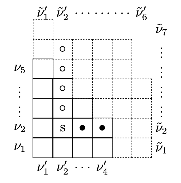
Figure 3: Arm length $A_{\tilde{Y}}(s)=4$ (white circles) and leg length $L_{Y}(s)=2$ (black dots) of a box at the site $s=(2,2)$ for the pair of superimposed diagrams $Y$ (solid lines) and $\tilde{Y}$ (dotted lines).

Note that they can be negative if the box $(i,j)$ are the coordinates of a box outside the tableau. Also, the previous formulae has to be evaluated at $\vec{\alpha}=(\alpha_{1},\alpha_{2})=(\alpha,-\alpha)$. The explicit expression for the NS function, a.k.a. classical Virasoro confluent conformal block $F$, is finally given by :

$$F(L)=\lim_{b\to 0}b^{2}\log\Lambda^{-\Delta}\mathfrak{F}\left(m_{3}/b,a_{i}/b,a/b,L/b\right)$$ (80)

Finally, let us comment on the symmetry properties discussed around Eq. (10). We start by proving that $F$ is invariant under $(m_{3},L)\to(-m_{3},-L)$. $F$ is defined in terms of (76), and the dependence on $(\mu,\Lambda)$ is entirely controlled by the irregular state. From (58) we see that the irregular state is invariant under $(\mu,\Lambda)\to(-\mu,-\Lambda)$, so the same must be true for the whole correlator. This property descends to the conformal blocks (76). In the semiclassical limit (80) this proves invariance of $F$ under $(m_{3},L)\to(-m_{3},-L)$.

We now prove symmetry properties of $F$ under permutation of masses. First of all note that

$$\sum_{\vec{Y}}\Lambda^{|\vec{Y}|}z_{\text{vec}}\left(\vec{\alpha},\vec{Y}\right)z_{\text{hyp}}\left(\vec{\alpha},\vec{Y},-\mu\right)\prod_{\theta=\pm}z_{\text{hyp}}\left(\vec{\alpha},\vec{Y},\alpha_{1}+\theta\alpha_{0}\right)$$ (81)

is symmetric under permutations of $(\alpha_{1}+\alpha_{0},\alpha_{1}-\alpha_{0},\mu)$. The only non symmetric term in (77) is the overall exponential term. However

$$\tilde{\mathfrak{F}}=e^{-\frac{1}{2}\mu\Lambda}\mathfrak{F}$$ (82)

has the permutation symmetry. Upon taking the semiclassical limit (80), this proves that $\tilde{F}$ as defined in (10) is symmetric under permutations of masses. Combining this property with symmetry under $(m_{3},L)\to(-m_{3},-L)$, finally proves that $\tilde{F}$ is symmetric under $(m_{i},L)\to(-m_{i},-L)$ for $i=1,2,3$.

Appendix C Appendix C: Proof of Large Frequency Behavior

We now present a CFT argument to prove the fact that at large $\omega$, the renormalized angular momentum becomes $a\approx 2iM\omega$ as indicated in (18) in the main text. We start from the correlator

$$e^{-\frac{1}{2}\Lambda\mu}\langle\mu,\Lambda|V_{\alpha_{1}}(1)|\Delta_{\alpha_{0}}\rangle\,$$ (83)

Exchanging $\mu$ and $\alpha_{0}+\alpha_{1}$ gives

$$e^{-\frac{1}{2}\Lambda(\alpha_{1}+\alpha_{0})}\langle(\alpha_{1}+\alpha_{0}),\Lambda|V_{\tilde{\alpha}_{1}}(1)|\Delta_{\tilde{\alpha}_{0}}\rangle\,.$$ (84)

where

$$\tilde{\alpha_{1}}=\frac{\mu_{3}+\alpha_{1}-\alpha_{0}}{2}\,,\quad\tilde{\alpha_{0}}=\frac{\mu_{3}-\alpha_{1}+\alpha_{0}}{2}\,.$$ (85)

Note that (83) and (84) define the same $\tilde{F}$. Defining as usual $\tilde{a}_{1,2}=\lim_{b\to 0}b\tilde{\alpha}_{1,2}$, the dictionary at large $\omega$ gives at leading order.

$$a_{1}+a_{0}\simeq\frac{-2iM\omega}{\kappa}\,,\quad\tilde{a}_{0}\simeq 2iM\omega\,,\quad\tilde{a}_{1}\simeq\mathcal{O}(1)\,.$$ (86)

$\tilde{a}_{1}$ is subleading with respect to the other parameters, therefore one can neglect the insertion at $1$ in (84). This gives

$$e^{-\frac{1}{2}\Lambda(\alpha_{1}+\alpha_{0})}\langle(\alpha_{1}+\alpha_{0}),\Lambda|V_{\tilde{\alpha}_{1}}(1)|\Delta_{\tilde{\alpha}_{0}}\rangle\simeq e^{-\frac{1}{2}\Lambda(\alpha_{1}+\alpha_{0})}\langle(\alpha_{1}+\alpha_{0}),\Lambda|\Delta_{\tilde{\alpha}_{0}}\rangle=e^{-\frac{1}{2}\Lambda(\alpha_{1}+\alpha_{0})}\Lambda^{\Delta}\,,$$ (87)

where we used the fact that $\langle\mu,\Lambda|\Delta_{i}\rangle=\Lambda^{\Delta_{i}}$. This gives for $\tilde{F}$

$$\tilde{F}\simeq=-\frac{L}{2}(a_{1}+a_{0})\,,$$ (88)

Inserting this in the Matone relation (6) we find the solution $a\simeq m_{3}$ (fixing to $+$ the $\pm$ ambiguity coming from the fact that (6) is quadraticin $a$). As a consistency condition note that this gives for $u$

$$u\simeq\frac{1}{2}-m_{3}^{2}+\frac{L}{2}(m_{3}-m_{1})\,,$$ (89)

consistently with the large $\omega$ limit of (5). Using (63) into (88) we finally recover (17) in the main text.

References

- Abbott et al. (2016) B. P. Abbott et al. (LIGO Scientific, Virgo), Phys. Rev. Lett. 116, 061102 (2016), arXiv:1602.03837 [gr-qc] .
- Akutsu et al. (2021) T. Akutsu et al. (KAGRA), PTEP 2021, 05A102 (2021), arXiv:2009.09305 [gr-qc] .
- Goldberger and Rothstein (2006) W. D. Goldberger and I. Z. Rothstein, Phys. Rev. D 73, 104029 (2006), arXiv:hep-th/0409156 .
- Rothstein (2014) I. Z. Rothstein, Gen. Rel. Grav. 46, 1726 (2014).
- Goldberger (2022a) W. D. Goldberger, (2022a), arXiv:2212.06677 [hep-th] .
- Goldberger (2022b) W. D. Goldberger, in 2022 Snowmass Summer Study (2022) arXiv:2206.14249 [hep-th] .
- Porto (2016) R. A. Porto, Phys. Rept. 633, 1 (2016), arXiv:1601.04914 [hep-th] .
- Kälin and Porto (2020) G. Kälin and R. A. Porto, JHEP 11, 106 (2020), arXiv:2006.01184 [hep-th] .
- Mogull et al. (2021) G. Mogull, J. Plefka, and J. Steinhoff, JHEP 02, 048 (2021), arXiv:2010.02865 [hep-th] .
- Cheung et al. (2018) C. Cheung, I. Z. Rothstein, and M. P. Solon, Phys. Rev. Lett. 121, 251101 (2018), arXiv:1808.02489 [hep-th] .
- Kosower et al. (2019) D. A. Kosower, B. Maybee, and D. O’Connell, JHEP 02, 137 (2019), arXiv:1811.10950 [hep-th] .
- Bern et al. (2019) Z. Bern, C. Cheung, R. Roiban, C.-H. Shen, M. P. Solon, and M. Zeng, (2019), arXiv:1908.01493 [hep-th] .
- Bern et al. (2020) Z. Bern, A. Luna, R. Roiban, C.-H. Shen, and M. Zeng, (2020), arXiv:2005.03071 [hep-th] .
- Buonanno et al. (2022) A. Buonanno, M. Khalil, D. O’Connell, R. Roiban, M. P. Solon, and M. Zeng, in Snowmass 2021 (2022) arXiv:2204.05194 [hep-th] .
- Cheung et al. (2023) C. Cheung, J. Parra-Martinez, I. Z. Rothstein, N. Shah, and J. Wilson-Gerow, (2023), arXiv:2308.14832 [hep-th] .
- Kosmopoulos and Solon (2023) D. Kosmopoulos and M. P. Solon, (2023), arXiv:2308.15304 [hep-th] .
- Bjerrum-Bohr et al. (2022) N. E. J. Bjerrum-Bohr, P. H. Damgaard, L. Plante, and P. Vanhove, J. Phys. A 55, 443014 (2022), arXiv:2203.13024 [hep-th] .
- Brandhuber et al. (2023a) A. Brandhuber, G. R. Brown, G. Chen, S. De Angelis, J. Gowdy, and G. Travaglini, (2023a), arXiv:2303.06111 [hep-th] .
- Herderschee et al. (2023) A. Herderschee, R. Roiban, and F. Teng, (2023), arXiv:2303.06112 [hep-th] .
- Elkhidir et al. (2023) A. Elkhidir, D. O’Connell, M. Sergola, and I. A. Vazquez-Holm, (2023), arXiv:2303.06211 [hep-th] .
- Georgoudis et al. (2023) A. Georgoudis, C. Heissenberg, and I. Vazquez-Holm, (2023), arXiv:2303.07006 [hep-th] .
- Caron-Huot et al. (2023) S. Caron-Huot, M. Giroux, H. S. Hannesdottir, and S. Mizera, (2023), arXiv:2308.02125 [hep-th] .
- Buonanno and Damour (1999) A. Buonanno and T. Damour, Phys. Rev. D 59, 084006 (1999), arXiv:gr-qc/9811091 .
- Buonanno and Damour (2000) A. Buonanno and T. Damour, Phys. Rev. D 62, 064015 (2000), arXiv:gr-qc/0001013 .
- Ronveaux (1995) A. Ronveaux, ed., Heun’s Differential Equations (The Clarendon Press Oxford University Press, New York, 1995) pp. xxiv+354.
- Bonelli et al. (2022) G. Bonelli, C. Iossa, D. P. Lichtig, and A. Tanzini, Phys. Rev. D 105, 044047 (2022), arXiv:2105.04483 [hep-th] .
- Nekrasov and Shatashvili (2009) N. A. Nekrasov and S. L. Shatashvili, in 16th International Congress on Mathematical Physics (2009) pp. 265–289, arXiv:0908.4052 [hep-th] .
- Bonelli et al. (2023) G. Bonelli, C. Iossa, D. Panea Lichtig, and A. Tanzini, Commun. Math. Phys. 397, 635 (2023), arXiv:2201.04491 [hep-th] .
- Dodelson et al. (2023) M. Dodelson, A. Grassi, C. Iossa, D. Panea Lichtig, and A. Zhiboedov, SciPost Phys. 14, 116 (2023), arXiv:2206.07720 [hep-th] .
- Aminov et al. (2023) G. Aminov, P. Arnaudo, G. Bonelli, A. Grassi, and A. Tanzini, JHEP 11, 059 (2023), arXiv:2307.10141 [hep-th] .
- Bianchi et al. (2022) M. Bianchi, D. Consoli, A. Grillo, and J. F. Morales, Phys. Lett. B 824, 136837 (2022), arXiv:2105.04245 [hep-th] .
- Bianchi and Di Russo (2023) M. Bianchi and G. Di Russo, JHEP 08, 217 (2023), arXiv:2212.07504 [hep-th] .
- Bianchi et al. (2023) M. Bianchi, G. Di Russo, A. Grillo, J. F. Morales, and G. Sudano, (2023), arXiv:2305.15105 [gr-qc] .
- Giusto et al. (2023) S. Giusto, C. Iossa, and R. Russo, JHEP 10, 050 (2023), arXiv:2306.15305 [hep-th] .
- Aminov et al. (2022) G. Aminov, A. Grassi, and Y. Hatsuda, Annales Henri Poincare 23, 1951 (2022), arXiv:2006.06111 [hep-th] .
- Consoli et al. (2022) D. Consoli, F. Fucito, J. F. Morales, and R. Poghossian, JHEP 12, 115 (2022), arXiv:2206.09437 [hep-th] .
- Fucito and Morales (2023) F. Fucito and J. F. Morales, (2023), arXiv:2311.14637 [gr-qc] .
- Mano et al. (1996a) S. Mano, H. Suzuki, and E. Takasugi, Prog. Theor. Phys. 96, 549 (1996a), arXiv:gr-qc/9605057 .
- Mano et al. (1996b) S. Mano, H. Suzuki, and E. Takasugi, Prog. Theor. Phys. 95, 1079 (1996b), arXiv:gr-qc/9603020 .
- Mano and Takasugi (1997) S. Mano and E. Takasugi, Prog. Theor. Phys. 97, 213 (1997), arXiv:gr-qc/9611014 .
- Sasaki and Tagoshi (2003) M. Sasaki and H. Tagoshi, Living Rev. Rel. 6, 6 (2003), arXiv:gr-qc/0306120 .
- Ivanov and Zhou (2022) M. M. Ivanov and Z. Zhou, (2022), arXiv:2209.14324 [hep-th] .
- Saketh et al. (2023) M. V. S. Saketh, Z. Zhou, and M. M. Ivanov, (2023), arXiv:2307.10391 [hep-th] .
- Casals and Ottewill (2015) M. Casals and A. C. Ottewill, Phys. Rev. D 92, 124055 (2015), arXiv:1509.04702 [gr-qc] .
- Casals et al. (2016) M. Casals, C. Kavanagh, and A. C. Ottewill, Phys. Rev. D 94, 124053 (2016), arXiv:1608.05392 [gr-qc] .
- Bautista et al. (2022) Y. F. Bautista, A. Guevara, C. Kavanagh, and J. Vinese, (2022), arXiv:2212.07965 [hep-th] .
- Teukolsky (1972) S. A. Teukolsky, Physical Review Letters 29, 1114 (1972).
- Teukolsky (1973) S. A. Teukolsky, The Astrophysical Journal 185, 635 (1973).
- Teukolsky and Press (1974) S. A. Teukolsky and W. Press, The Astrophysical Journal 193, 443 (1974).
- Batic and Schmid (2007) D. Batic and H. Schmid, J. Math. Phys. 48, 042502 (2007), arXiv:gr-qc/0701064 .
- Flume et al. (2004) R. Flume, F. Fucito, J. F. Morales, and R. Poghossian, JHEP 04, 008 (2004), arXiv:hep-th/0403057 .
- Matone (1995) M. Matone, Phys. Lett. B 357, 342 (1995), arXiv:hep-th/9506102 .
- Arnaudo et al. (2022) P. Arnaudo, G. Bonelli, and A. Tanzini, (2022), arXiv:2212.06741 [hep-th] .
- Alday et al. (2010) L. F. Alday, D. Gaiotto, and Y. Tachikawa, Lett. Math. Phys. 91, 167 (2010), arXiv:0906.3219 [hep-th] .
- (55) See ancillary files for this manuscript.
- Page (1976a) D. N. Page, Phys. Rev. D 13, 198 (1976a).
- Page (1976b) D. N. Page, Phys. Rev. D 14, 3260 (1976b).
- Saketh et al. (2022) M. V. S. Saketh, J. Steinhoff, J. Vines, and A. Buonanno, (2022), arXiv:2212.13095 [gr-qc] .
- Levi and Steinhoff (2015) M. Levi and J. Steinhoff, JHEP 09, 219 (2015), arXiv:1501.04956 [gr-qc] .
- Gorsky et al. (2018) A. Gorsky, A. Milekhin, and N. Sopenko, JHEP 01, 133 (2018), arXiv:1712.02936 [hep-th] .
- Lisovyy and Naidiuk (2022) O. Lisovyy and A. Naidiuk, J. Phys. A 55, 434005 (2022), arXiv:2208.01604 [math-ph] .
- (62) “Black Hole Perturbation Toolkit,” (bhptoolkit.org).
- Kol and Smolkin (2012) B. Kol and M. Smolkin, JHEP 02, 010 (2012), arXiv:1110.3764 [hep-th] .
- Landau and Lifshits (1991) L. D. Landau and E. M. Lifshits, Quantum Mechanics: Non-Relativistic Theory, Course of Theoretical Physics, Vol. v.3 (Butterworth-Heinemann, Oxford, 1991).
- Dolan (2008) S. R. Dolan, Class. Quant. Grav. 25, 235002 (2008), arXiv:0801.3805 [gr-qc] .
- (66) M. M. Ivanov, Y.-Z. Li, J. Parra-Martinez, and Z. Zhou, in preparation .
- Bautista et al. (2021) Y. F. Bautista, A. Guevara, C. Kavanagh, and J. Vines, (2021), arXiv:2107.10179 [hep-th] .
- Bern et al. (2022) Z. Bern, D. Kosmopoulos, A. Luna, R. Roiban, and F. Teng, (2022), arXiv:2203.06202 [hep-th] .
- Aoude et al. (2022a) R. Aoude, K. Haddad, and A. Helset, JHEP 07, 072 (2022a), arXiv:2203.06197 [hep-th] .
- Aoude et al. (2022b) R. Aoude, K. Haddad, and A. Helset, Phys. Rev. Lett. 129, 141102 (2022b), arXiv:2205.02809 [hep-th] .
- Chiodaroli et al. (2022) M. Chiodaroli, H. Johansson, and P. Pichini, JHEP 02, 156 (2022), arXiv:2107.14779 [hep-th] .
- Haddad (2023) K. Haddad, (2023), arXiv:2303.02624 [hep-th] .
- Cangemi et al. (2022) L. Cangemi, M. Chiodaroli, H. Johansson, A. Ochirov, P. Pichini, and E. Skvortsov, (2022), arXiv:2212.06120 [hep-th] .
- Cangemi et al. (2023) L. Cangemi, M. Chiodaroli, H. Johansson, A. Ochirov, P. Pichini, and E. Skvortsov, (2023), arXiv:2311.14668 [hep-th] .
- Guevara et al. (2019) A. Guevara, A. Ochirov, and J. Vines, JHEP 09, 056 (2019), arXiv:1812.06895 [hep-th] .
- Chung et al. (2019) M.-Z. Chung, Y.-T. Huang, J.-W. Kim, and S. Lee, JHEP 04, 156 (2019), arXiv:1812.08752 [hep-th] .
- Bautista and Guevara (2019) Y. F. Bautista and A. Guevara, (2019), arXiv:1903.12419 [hep-th] .
- Bautista and Siemonsen (2022) Y. F. Bautista and N. Siemonsen, JHEP 01, 006 (2022), arXiv:2110.12537 [hep-th] .
- Chen et al. (2022) W.-M. Chen, M.-Z. Chung, Y.-t. Huang, and J.-W. Kim, JHEP 08, 148 (2022), arXiv:2111.13639 [hep-th] .
- Bjerrum-Bohr et al. (2023) N. E. J. Bjerrum-Bohr, G. Chen, and M. Skowronek, (2023), arXiv:2302.00498 [hep-th] .
- Alessio (2023) F. Alessio, (2023), arXiv:2303.12784 [hep-th] .
- De Angelis et al. (2023) S. De Angelis, R. Gonzo, and P. P. Novichkov, (2023), arXiv:2309.17429 [hep-th] .
- Aoude et al. (2023) R. Aoude, K. Haddad, C. Heissenberg, and A. Helset, (2023), arXiv:2310.05832 [hep-th] .
- Brandhuber et al. (2023b) A. Brandhuber, G. R. Brown, G. Chen, J. Gowdy, and G. Travaglini, (2023b), arXiv:2310.04405 [hep-th] .
- Glampedakis and Andersson (2001) K. Glampedakis and N. Andersson, Class. Quant. Grav. 18, 1939 (2001), arXiv:gr-qc/0102100 .
- Fioravanti and Gregori (2021) D. Fioravanti and D. Gregori, (2021), arXiv:2112.11434 [hep-th] .
- Fioravanti et al. (2022) D. Fioravanti, D. Gregori, and H. Shu, (2022), arXiv:2208.14031 [hep-th] .
- Aoude and Ochirov (2023) R. Aoude and A. Ochirov, (2023), arXiv:2307.07504 [hep-th] .
- Jones and Ruf (2023) C. R. T. Jones and M. S. Ruf, (2023), arXiv:2310.00069 [hep-th] .
- Chen et al. (2023) Y.-J. Chen, T. Hsieh, Y.-T. Huang, and J.-W. Kim, (2023), arXiv:2312.04513 [hep-th] .
- Scheopner and Vines (2023) T. Scheopner and J. Vines, (2023), arXiv:2311.18421 [gr-qc] .
- Loutrel et al. (2021) N. Loutrel, J. L. Ripley, E. Giorgi, and F. Pretorius, Phys. Rev. D 103, 104017 (2021), arXiv:2008.11770 [gr-qc] .
- Ripley et al. (2021) J. L. Ripley, N. Loutrel, E. Giorgi, and F. Pretorius, Phys. Rev. D 103, 104018 (2021), arXiv:2010.00162 [gr-qc] .
- Teschner (2001) J. Teschner, Class. Quant. Grav. 18, R153 (2001), arXiv:hep-th/0104158 .
- Gaiotto (2013) D. Gaiotto, J. Phys. Conf. Ser. 462, 012014 (2013), arXiv:0908.0307 [hep-th] .
- Bonelli et al. (2012) G. Bonelli, K. Maruyoshi, and A. Tanzini, JHEP 02, 031 (2012), arXiv:1112.1691 [hep-th] .
- Gaiotto and Teschner (2012) D. Gaiotto and J. Teschner, JHEP 12, 050 (2012), arXiv:1203.1052 [hep-th] .
- Belavin et al. (1984) A. A. Belavin, A. M. Polyakov, and A. B. Zamolodchikov, Nucl. Phys. B 241, 333 (1984).
- Zamolodchikov and Zamolodchikov (1996) A. B. Zamolodchikov and A. B. Zamolodchikov, Nucl. Phys. B 477, 577 (1996), arXiv:hep-th/9506136 .
- Dorn and Otto (1994) H. Dorn and H. J. Otto, Nucl. Phys. B 429, 375 (1994), arXiv:hep-th/9403141 .
- Flume and Poghossian (2003) R. Flume and R. Poghossian, Int. J. Mod. Phys. A 18, 2541 (2003), arXiv:hep-th/0208176 .
- Bruzzo et al. (2003) U. Bruzzo, F. Fucito, J. F. Morales, and A. Tanzini, JHEP 05, 054 (2003), arXiv:hep-th/0211108 .