ConSequence: Synthesizing Logically Constrained Sequences for Electronic Health Record Generation
Abstract
Generative models can produce synthetic patient records for analytical tasks when real data is unavailable or limited. However, current methods struggle with adhering to domain-specific knowledge and removing invalid data. We present ConSequence, an effective approach to integrating domain knowledge into sequential generative neural network outputs. Our rule-based formulation includes temporal aggregation and antecedent evaluation modules, ensured by an efficient matrix multiplication formulation, to satisfy hard and soft logical constraints across time steps. Existing constraint methods often fail to guarantee constraint satisfaction, lack the ability to handle temporal constraints, and hinder the learning and computational efficiency of the model. In contrast, our approach efficiently handles all types of constraints with guaranteed logical coherence. We demonstrate ConSequence’s effectiveness in generating electronic health records, outperforming competitors in achieving complete temporal and spatial constraint satisfaction without compromising runtime performance or generative quality. Specifically, ConSequence successfully prevents all rule violations while improving the model quality in reducing its test perplexity by 5% and incurring less than a 13% slowdown in generation speed compared to an unconstrained model.
Introduction
Sequential data generation applications are used in various fields, such as healthcare (Choi et al. 2017; Biswal et al. 2021; Zhang et al. 2021; Theodorou, Xiao, and Sun 2023), finance (Assefa et al. 2020; Dogariu et al. 2022), natural language processing (Gatt and Krahmer 2018; Dong et al. 2022; Reiter and Dale 1997), and computer vision (Tulyakov et al. 2018; Yang, Srivastava, and Mandt 2022; Ho et al. 2022). In these applications, generative models demonstrate the capability to produce synthetic data closely resembling real-world datasets. Notably, language models have showcased remarkable achievements in domains like text generation (Chowdhery et al. 2022; Thoppilan et al. 2022; Brown et al. 2020) and health record generation (Theodorou, Xiao, and Sun 2023), primarily attributed to their adeptness in accurate next-token forecasting. Beyond mimicking real data, generative models often require adhering to specific rules and temporal dependencies unique to an application domain. For instance, in medicine, generative models should follow logical constraints such as indications (the reason for using a specific treatment for a disease) and contraindications (the reason that makes a particular treatment inadvisable for that disease) to create realistic sequential data.
To support domain-specific applications, generated samples must not only approximate the true underlying data distribution but also encapsulate the relationships and dependencies encoded as rules derived from external knowledge. Failing to meet these constraints can hinder efficacy and deter adoption. Various current approaches attempt to ensure logical consistency in neural network outputs. These methods encompass strategies such as integrating rule constraints into the loss function (Xu et al. 2018; Fischer et al. 2019), employing post-processing modules designed to rectify model output violations (Manhaeve et al. 2018; Hoernle et al. 2022; Ahmed et al. 2022), or directly adding model components that ensure the final weights and outputs align with domain knowledge (Towell and Shavlik 1994; Avila Garcez and Zaverucha 1999; Giunchiglia and Lukasiewicz 2021). Despite the existing effort in constraint enforcement, sequential data generation still faces several challenges in aligning with real-world knowledge.
-
•
Inadequate treatment of temporal logical constraints. Existing models struggle with temporal constraints, which can be static or evolve across multiple time steps. These constraints are key to enhancing accuracy and reliability in sequential generation models. Yet, no existing models effectively manage these constraints as the information conditioning them may not be accessible at each time step.
-
•
Efficiency and scalability. Sequential tasks typically encompass a multitude of time steps and entail a substantial output dimensionality, underscoring the need for a streamlined approach to facilitate large-scale sequence generation. Current methods can be slow and computationally demanding, impairing real-world generation speed (Bond-Taylor et al. 2021). Thus, an effective solution should not only be asymptotically efficient but also maintain high generation speeds for practical use.
-
•
Difficulty in achieving full logical consistency. Realism in sequential data generation is paramount, but logical inconsistencies can compromise it. Hence, encoding domain knowledge without error is essential. For full trustworthiness, methods must uphold all logical constraints; even one violation can erode user confidence. This is especially vital in critical areas like healthcare.
In this paper, we present a method called ConSequence for addressing the challenges of sequential constrained knowledge infusion. ConSequence can handle entailment formatted rules with both soft and hard logical constraints, covering static, temporal, and combined antecedents.
-
•
Temporal antecedent compilation via attentive history aggregation. We employ an attention-based temporal aggregator for effectively consolidating historical data at each time step, supporting both absolute and relative aggregation while accommodating sequence variations.
-
•
Deterministic constraint execution via rule neuron. We introduce a graphical module that verifies each antecedent component, providing absolute constraint satisfaction.
-
•
Parallel constraint application via efficient GPU implementation. We represent the mentioned components as weight matrices. These are then seamlessly incorporated as a constraint head in neural network models, processing many rules and records in parallel, resulting in minimal to no GPU slowdown and maximizing overall efficiency.
To assess its effectiveness, we undertake a series of experiments on a benchmark task employing the cutting-edge health record generation model, HALO (Theodorou, Xiao, and Sun 2023), across two real-world datasets. We benchmark our method against prevailing constraint enforcement approaches, evaluating them on: (1) rule violation count, (2) overall model quality, and (3) generative efficiency.
Our results demonstrate that ConSequence outperforms all other methods over all three criteria. While most baselines result in over 25% of their generated records for one dataset being invalid, ConSequence successfully prevents any rule violations. Furthermore, ConSequence improves the model quality and incurs less than a 13% slowdown in generation speed compared to an unconstrained model. In comparison, all of the baselines that are not loss-based exhibit slowdowns exceeding 37%, with the majority performing even more poorly. This highlights the effectiveness of ConSequence for generating high-quality health records while satisfying domain-specific constraints.
Related Work
Various strategies have been proposed to apply logical constraints to neural network models, especially in multi-label predictions (Dash et al. 2022; Giunchiglia, Stoian, and Lukasiewicz 2022). One method is to include logical constraints in the loss function during training, as regularization or penalty terms (Xu et al. 2018; Fischer et al. 2019). Another approach involves adjusting the model’s weights to satisfy the constraints (Towell and Shavlik 1994; Avila Garcez and Zaverucha 1999; Ahmed et al. 2022). Alternatively, some techniques focus on mapping the model’s outputs to meet the constraints (Manhaeve et al. 2018; Hoernle et al. 2022; Giunchiglia and Lukasiewicz 2021).
Despite the range of approaches, the ultimate goal is consistent: to ensure the model’s outputs align with logical constraints, enhancing interpretability and trustworthiness. While progress has been made in applying constraint methods to various applications, adapting these techniques to our specific task faces challenges. For instance, loss-based approaches (Xu et al. 2018; Fischer et al. 2019) reduce constraint violations but do not guarantee logical consistency, potentially limiting practical use for our needs. Additionally, certain methods ensuring consistency (Giunchiglia and Lukasiewicz 2021; Hoernle et al. 2022) can be slow, which might not suit large-scale sequential generation settings.
Moreover, our task involves integrating temporal rules that may change over time, without their logical precursors necessarily present at each step. Although some methods have applied constraints to sequential text and molecule data (Hokamp and Liu 2017; Liu et al. 2020), none have specifically addressed the challenge of satisfying general temporal logical constraints efficiently. This highlights the need for innovative approaches capable of handling complex temporal constraints in a computationally efficient manner.
Problem Formulation
We present the problem formulation for the task of longitudinal patient record generation. We first define patient data.
Definition 1 (Sequential Patient Health Record Data).
A patient record is a time-sequenced series of visits, denoted as . Each visit, , consists of a variable number of unique medical codes from a set . These codes, , encode medical information such as diagnoses, procedures, and medications.
To prepare for machine learning models, we transform into a matrix representation for a patient with visits. Each visit is a multi-hot binary vector, with representing the presence of the -th code in the -th visit of . Static features such as gender, ethnicity, and birth year are encoded in the first visit .
In synthetic patient generation, our aim is to create synthetic patient sequences from scratch, given a real patient dataset to train on, that mimic real records and offer equivalent downstream utility. We incorporate real-world knowledge through logical constraints to guide generation. These constraints, defined as a series of logical entailment statements over codes and visits, may be grounded in a single time step or span multiple time steps. We encode them in a format called Conjunctive Implicative Form.
Definition 2 (Conjunctive Implicative Form).
A statement is in Conjunctive Implicative Form (CIF) if it is of the form for , where is a literal such that or for a variable .
Encoding Rules. Our set of variables consists of generated codes across all timesteps, that is, all . We let denote either of and . Given this, our rules must be in one of the following formats.
-
1.
, a rule with an empty antecedent, though this does not generally appear in practice.
-
2.
, represents a hierarchical relationship: a specified truth value of necessitates one of . For example, if a patient is taking insulin, they must have diabetes.
-
3.
, which extends the former to relate the truth value of a boolean combination of terms to that of a singular term. For example, if a patient has heart disease and takes a statin, they must have high cholesterol.
-
4.
, a temporal rule relating the prior timestep and current time. For example, lifelong diseases like diabetes will always continue to appear once they begin.
-
5.
, a boolean combination of terms across a set of specified previous timesteps, , which relate to the current time. For example, a patient without a past history of pregnancy can’t have complications during childbirth.
-
6.
, relating a boolean combination of terms across both past and current timesteps to a singular boolean variable . For example, a patient with past diabetes and current numbness in their feet must have diabetic peripheral neuropathy.
Each rule consists of a temporal component which determines the indices of the past time steps referred to, the variables in the past and present which condition the output, and the output literal111We assume rules are acyclic but make no additional assumptions, and this approach can be generalized to cyclic rules with an initial transformation and elimination step, not discussed here.. If a rule has a non-empty temporal component, we classify it as temporal, and we otherwise consider it to be static. We use entailment statements with conjunctive antecedents to represent rules, offering conciseness, efficient processing, and aligning with logical constraints in real-world settings. In contrast, other models (Xu et al. 2018; Hoernle et al. 2022) use logical normal forms combining variables with AND, OR, or entailment connectors, which can be cumbersome for large outputs, without additional representational benefits. Next we show that our entailment-based format equals the representational power of alternative encoding schemes.
Theorem 1.
Given a boolean expression in conjunctive normal form, there exists an equivalent set of statements in conjunctive implicative form.
Proof.
An expression in conjunctive normal form is the conjunction of one or more clauses , where each clause is the disjunction of one or more literals . Given an expression in conjunctive normal form, we proceed as follows. First, we convert each clause to to the equivalent statement . Applying De Morgan’s Laws, we can further convert this to the statement in conjunctive implicative form . That is, the converted expression is now the conjunction of conjunctive implicative statements. Within our format, the conjunction of statements is implicitly represented through their mutual presence within a set, so is logically equivalent to the set of statements in conjunctive implicative form formed through this conversion. ∎
ConSequence Method
We introduce our ConSequence method (seen in Figure 1) for generating logically constrained sequential data. ConSequence is designed to directly mirror the logical entailment process. It involves two modules: temporal aggregation and antecedent evaluation, followed by a matrix multiplication-based approach for efficient parallel constraint application optimized for modern GPU architectures.
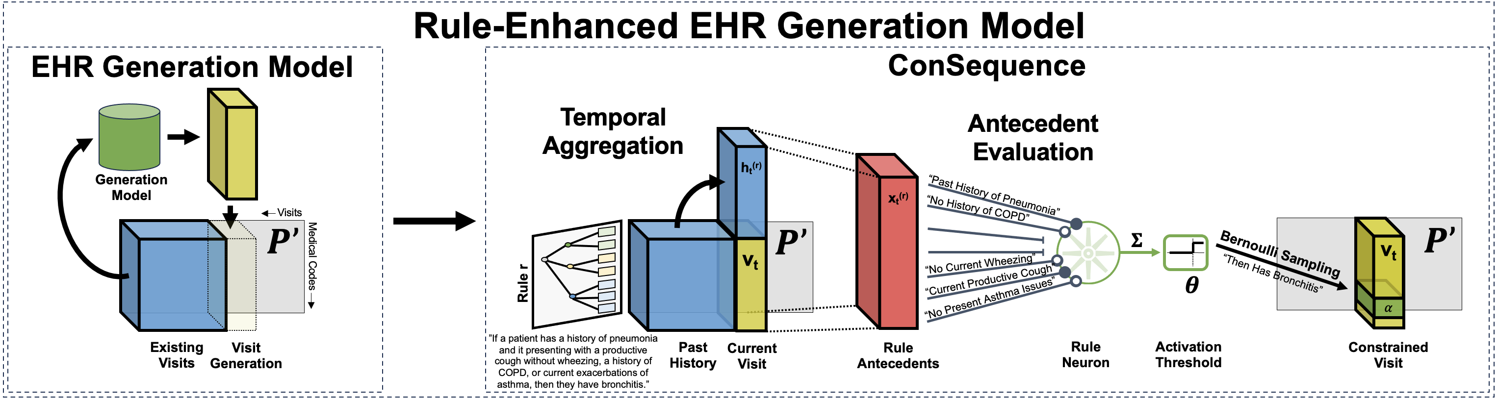
A. Temporal Aggregation
To support temporal rules, we first conduct temporal sequence aggregation. Specifically, given the sequence of all visits , where is the visit at time , we consider a temporal rule that contains a temporal component . refers to the set of indices of past time steps whose visits are referenced within , and may be both absolutely (e.g. the second time step) and relatively (e.g. the previous time step) numbered, where we represent relative numberings as negative indices. We define as a function that maps a time step to a set of referenced past time steps using , converting relatively numbered visits to absolutely numbered ones and handling the inability of time steps to reference themselves and future visits as a part of their past history. For example, if , then we have . Next, we aggregate the relevant past visits according to . We define binary mask vector which varies across both rules and time steps:
| (1) |
We then construct the aggregated history representation for time step and rule by:
| (2) |
Here, denotes the boolean OR operation, and is a static vector that aggregates the relevant codes within past visits according to the temporal component . This allows us to aggregate past sequences into fixed representations for each time step and rule, which are treated as standard variables for the entailment calculation in the next module.
B. Antecedent Evaluation
Once we have , we turn the problem into a standard entailment constraint problem. We solve this problem using a recurrent neuron model to evaluate the antecedent of a logical entailment and set the consequent. Each logical rule is constructed as a neuron, inspired by activation thresholds in biological and machine learning processes (Lin 2017), that only activates when all antecedent literals are satisfied, feeding back into the input to set the consequent.
Construction of the Rule Neuron
Let the variables that the rule operates over be represented by the binary vector which consists of both the aggregated historical variables and current visit representation. The antecedent of one of our logical entailment rules is defined as a conjunction of literals, each of the form or , referring to -th element of . Let be the set of such literals in the antecedent which refer collectively to a subset of . The rule neuron accepts inputs from the variables in and is constructed as follows: we denote the weight of the connection between the neuron and the -th variable in as and set it to if the variable is in and if its negation is in . For all other variables, the weight is set to 0. This construction is based on the logical interpretation of the antecedent, where the presence of a variable in the antecedent implies its positive contribution to the truth value, and the presence of its negation implies its negative contribution. More explicitly, we set the neuron’s weights by:
| (3) |
For instance, consider a rule stipulating that patients with past history of gastric ulcer and current symptom of melena, without past colorectal cancer, current hematemesis, or current esophageal varices must have gastrointestinal bleeding. The weights corresponding to the variables for past gastric ulcer and current melena in would be 1 while the variables for past colorectal cancer, current hematesis, and current esophageal varices to -1. All others would be 0.
Activation Process
Given the constructed neuron, we use it as follows. We first set the activation threshold to the number of positive, non-negated variables (of the form rather than ) in . Given , the activation process begins. The weighted sum of the inputs is calculated by Eq. (4):
| (4) |
If the is greater than or equal to , the neuron fires and sets the output variable in to the output value, . Otherwise, it remains inactive. It’s important to note that, based on the construction, is reached only if all of the positive variables and none of the negations are found in the input. For instance, using the previously mentioned example rule, would be set to 2. would then equal 2 only if the variables for past gastric ulcer and current melena are both 1 in , as they are the sole potential positive contributions during the activation sum. Furthermore, the variables for past colorectal cancer, current hematesis, and current esophageal varices must all be 0 to avoid any reduction below 2 due to their corresponding weight of -1.
Handling Soft Constraints
We also want to support settings where is a soft constraint with between 0 and 1. This flexibility is essential when the relation between variables is probabilistic. For example, most cases of COPD involve a past history of smoking, but exceptions do exist. So, we might include a rule stating that a patient without a past history of smoking has just a 1% chance of presently showing COPD and set accordingly. To address such cases, we add a final step before setting the output variable in . During training, we set the variable to the correct probability, but the output variables must equal 0 or 1 during generation. To achieve this, we sample from a Bernoulli distribution with probability before setting the value, resulting in a binary output while satisfying soft constraints by aligning that output with the proper underlying probabilities. Note that we can also apply this sampling process to hard constraints because sampling from and always yield 0 and 1, respectively. Therefore, we can integrate this sampling process into our core activation process without special handling for different constraints types.
Rule Evaluation
The rule evaluation process involves encoding the temporal history of each binary variable and feeding them, along with the current variables, to the rule neuron. The rule neuron evaluates the antecedent by computing the weighted sum of its inputs, comparing it to the activation threshold, and activating the neuron if the threshold is reached. If the neuron fires, it overrides any modeling by the preceding architecture and sets the output variable to the mandated output value, sampling from that value if during generation as opposed to training, as in Eq. (5):
| (5) |
This end-to-end process can be seen in Figure 1.
C. Parallel Constraint Application
In the previous sections, we have presented ConSequence in the context of a single rule and, in most cases, a single time step. During generation, we will only be concerned with the most recent visit at any given step, but during training it will be valuable to constrain all time steps simultaneously. Furthermore, applying multiple rules simultaneously is valuable for improving efficiency in any setting. So, we present a matrix multiplication formulation of ConSequence that leverages modern GPU computing architectures to simultaneously and efficiently apply groups of rules across time steps and across batches of patient records.
Rule Grouping and Combination
We begin by organizing rules into distinct groups, denoted as where each group contains a set of rules that can be processed simultaneously. While the temporal aggregation module prevents the combination of rules with different temporal components, we note that most rules use one of a few common components such as the first visit, the previous visit, or all past history. With this in mind, we categorize rules according to their temporal components.
We can then combine rules in each category of temporal components into rule groups if they have different output variables and their antecedent variables do not include output variables from previous rules in the same category. To do this, we iterate through the rules of each category, adding them to the current group and starting a new group each time we encounter a rule whose input or output variables overlaps with the output of a preceding rule in the current group.
Temporal Aggregation
To perform temporal aggregation across a group of rules, , with a shared temporal component, we use a technique inspired by masked self-attention. It involves constructing a temporal mask matrix , where each row is a binary vector that determines which other time steps the -th time step can attend to. Specifically, each in is set by Eq. (6):
| (6) |
By employing boolean matrix multiplication, we compute using the patient record by , where each row is the aggregated temporal history vector introduced previously (for any ).
Rule Execution and Output
This aggregated temporal history matrix can then be concatenated along the code dimension to to form . We then construct matrix to represent the rule neuron weights. For each rule in the group, we set the values in the column corresponding to the output code based on the construction of detailed earlier. Note that since there is no overlap in output variables within a group, each column is constructed without interference between different rules.
Utilizing matrix multiplication, we compute the antecedent sum output , resulting in a matrix where each value whose row corresponds to time step and whose column corresponds to the output variable in rule is equal to the sum from earlier. This value is a count of how many positive literals in the corresponding antecedent were satisfied at that time step minus how many negatives were failed (0 if there was no rule corresponding to that variable). When this count is equal to the number of positive literals, , we set the output code to the output value, . As we have multiple and values per group, we combine the constants into vectors (setting values corresponding to output codes which are not used in the rule group to -1 so that the equality is never satisfied) and respectively which may perform comparison and instantiations element-wise in parallel. To support both hard and soft constraints simultaneously, we can also first sample from the Bernoulli distribution defined by and set the output code to the resulting binary values. As a single step equation, this process can be summarized:
| (7) |
where the group of rules are applied simultaneously over all time steps and all records in a batch, effectively enabling parallel enforcement of rules.
| Outpatient | Inpatient | |
| # Records | 1,006,321 | 46,520 |
| Mean Visits/Record | 35.40 | 1.27 |
| Mean Codes /Visit | 1.69 | 13.61 |
| # Phecodes | 1,817 | 1,610 |
| Demographic | 7 | 6 |
| Violations on Outpatient Dataset | Violations on Inpatient Dataset | |||||
| Static | Temporal | % Valid | Static | Temporal | % Valid | |
| Vanilla HALO | 1265.4 (18.1) | 17.5 (2.9) | 87.2% (0.002) | 4320.6 (22.2) | 2046.2 (35.6) | 65.4% (0.002) |
| Post Processing | 0.0 | 0.0 | 100% | 0.0 | 0.0 | 100.0% |
| Semantic Loss | 955.5 (9.2) | 18.7 (3.6) | 90.3% (0.001) | 3827.0 (23.3) | 1817.2 (28.8) | 65.3% (0.002) |
| CCN | 1013.6 (15.0) | 17.7 (2.1) | 91.0% (0.001) | 3070.24 (18.3) | 2149.76 (32.5) | 70.7% (0.002) |
| MultiPlexNet | 0.0 | 2714.2 (3.6) | 89.7% (0.001) | 0.0 | 3304.8 (20.1) | 72.7% (0.002) |
| SPL | 0.0 | 41 | 99.9% | 0.0 | 11.5 (1.4) | 99.9% (0.0001) |
| ConSequence | 0.0 | 0.0 | 100% | 0.0 | 0.0 | 100% |
D. Runtime Analysis
ConSequence can process, evaluate, and adhere to rules in running time. We include a proof in our supplement, but the outline involves breaking the process down into its smaller components, analyzing the time to aggregate the history, generate the rule neuron, perform the entailment calculation, and set the output variables.
E. Training and Generation Process
We conclude our presentation of ConSequence by outlining how it works with the underlying generative architecture. ConSequence is designed to integrate seamlessly into any underlying sequentially generating architecture. During both training and generation, the process involves feeding the patient record input into the underlying model to predict the probabilities of the variables in the next visit before updating those probabilities via the ConSequence module.
During training, the true binary labels for the predicted visits are used as inputs to ConSequence. The antecedent evaluation process updates the model’s predicted probabilities based on logical constraints. The enhanced model’s predictions, now incorporating constraint-driven logic, can then be compared to the ground truth labels, allowing for the calculation of a loss value that guides the model’s training process without having to worry about learning prior
During generation, the underlying model predicts the probabilities for the next visit based on the current record, and a full, binary visit is sampled from those probabilities. The predicted visit is then passed through ConSequence, which enforces the logical constraints. This ensures that the generated sequence adheres to the desired constraints while still being synthesized by the underlying architecture.
So, ConSequence enhances the underlying generative architecture by incorporating logical constraints seamlessly into both the training and generation processes. This enables the end-to-end training of a stronger model and the generation of logically constrained sequential data that maintains clinical coherence while meeting specific requirements.
Experiments
Experimental Setting
We evaluate ConSequence against state-of-the-art constraint enforcement approaches by applying each to the HALO (Theodorou, Xiao, and Sun 2023) architecture (as one exemplar for these model agnostic techniques) for synthetic EHR generation. We perform a series of experiments on a pair of underlying real-world EHR datasets. Below are details concerning our data, baselines, and experimental design with remaining information found in our supplement.
Datasets
We used an outpatient EHR dataset from real-world US claims data and an inpatient EHR dataset from the public MIMIC-III dataset. Both datasets represent patients as visits. We encoded gender and age categories into the patient matrix representation using binary variables and added a “label visit” with only this demographic information at the beginning of each set of visits. This enables us to condition subsequent medical codes by the patient’s gender or age. Each dataset contains visits with ICD-9 diagnosis codes that we aggregated to higher level codes based on their respective ontologies. For instance, we combined diagnosis codes based on initial letter and first two digits (e.g., A24, A24.1, and A24.25 are aggregated to A24). We also limited each patient to a max of 100 visits, which removed very few visits in practice. Table 1 provides the statistics of the final datasets. Additional details are available in the supplement.
Rules
Although we expect experts to provide most rules in practice, we generated them in a data-driven approach here.
We identify static rules as: 1) For each demographic category, we permit at most one variable to be set (or none if unknown). Thus, autoregressive rules were added to prevent setting subsequent variables if a previous one was already set. 2) We identify pairs of codes that exclusively co-occur. For each pair, we establish a rule mandating the presence of the first code whenever the second one is present.
We identify temporal rules as follows: 1) We identify prevalent codes that never appear within a demographic category. For each demographic category, we establish a rule disallowing these codes if the corresponding demographic variable is set in the first visit. 2) We detect common codes that only occur following a specific code. In each instance, we impose a rule preventing the former code unless the latter has previously occurred. 3) We find frequent codes that consistently appear in subsequent visits once they’ve occurred. For each case, we formulate a rule necessitating the code in the current visit if it was present in the previous one.
Our final rule sets consist of 71 rules (14 static, 57 temporal) for the outpatient dataset and 95 (11 static, 84 temporal) for the inpatient dataset. More details about cutoffs, counts by type, and some examples can be found in the appendix.
Baselines
We compare our method with several baseline approaches for handling logical constraints.
-
•
Post Processing is a naive approach removing any generated samples violating the constraints and generates more samples to replace them. It guarantees consistency with the constraints but is slower due to repeated generation and rule-checking, and may incur distribution shifts.
-
•
Semantic Loss (Xu et al. 2018) is a regularization method based on the probability of breaking a constraint. It can handle temporal rules but does not guarantee compliance.
-
•
CCN (Giunchiglia and Lukasiewicz 2021) is a rule-based method that uses maximum and minimum operations to set the output based on the values of the inputs in the antecedent. It guarantees compliance but cannot handle temporal rules or any where the output variable is set to 0.
-
•
MultiPlexNet (Hoernle et al. 2022) introduces a categorical latent variable to select between satisfying assignments of constraints. It guarantees the satisfaction of static rules but does not support temporal constraints.
-
•
Semantic Probability Layer (SPL) (Ahmed et al. 2022) constructs probabilistic circuits to handle a wide variety of constraints. It can handle any static but no temporal rules222We modified both the SPL and corresponding HALO model for partial compatibility with our setting but couldn’t achieve full capabilities. Further details are available in the supplement..
Implementation
We train HALO models on both datasets and apply each constraint enforcement method in turn. We generate a synthetic dataset of 10,000 patients from scratch with each method and without any constraints for comparison. These generations are performed on identical hardware (a single Tesla P100 GPU), and the generation process is repeated 25 times for each method (except for SPL on the outpatient dataset as it takes too long) to validate our results.
Results on the Evaluation of Logical Adherence
Our first evaluation measures each method’s effectiveness in preventing rule violations. We count rule violations within the synthetic datasets, stratified by rule type, and calculate the percentage of fully valid generated patients.
Table 2 presents these statistics, highlighting that ConSequence is the only non-post-processing method guaranteeing full prevention of rule violations. Although CCN, MultiPlexNet, and SPL adhere to some static rules and Semantic Loss regularizes all constraints, no baseline methods fully satisfy temporal rules, leading to numerous invalid generations. In contrast, ConSequence manages all rule types, preventing invalid generations more efficiently than the naive Post Processing approach.
Results on the Evaluation of Data Enrichment
This section assesses whether knowledge infusion impacts learning and generation by evaluating the quality of the model and its synthetic data. We first calculate the model’s perplexity on a held-out test set, which signifies the log probability of the test set, normalized by the number of codes in the dataset. Lower perplexity values indicate superior performance. Table 3 displays the perplexities for each method on each dataset. We find that ConSequence enhances the model’s performance on both datasets by eliminating error sources from predicted rule violations, allowing for absolute non-violation predictions, and facilitating the model to learn dataset patterns during training beyond the rules. ConSequence exhibits the most significant improvement, while CCN and Semantic Loss moderately enhance learning. In contrast, MultiPlexNet and SPL baselines hinder the modeling of the underlying data distribution by introducing more complex loss formulations during training.
| Outpatient | Inpatient | |
| Vanilla HALO | 24.019 | 13.443 |
| Semantic Loss | 23.995 | 13.432 |
| CCN | 23.976 | 12.985 |
| MultiPlexNet | 119.560 | 24.260 |
| SPL | 34.454 | 22.794 |
| ConSequence | 23.924 | 12.712 |
We also evaluated the realism of the generated dataset by comparing the probabilities of codes and their combinations in each synthetic dataset to their original training datasets, and we provide those results in our supplement.
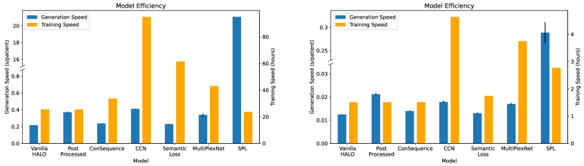
Results on Method Efficiency
The final evaluation checks if ConSequence maintains robust real-world efficiency. Figure 2 presents the training and generation speeds for each model. Our results highlight that ConSequence provides commendable real-world efficiency. It outpaces other constraint methods during training, while the baselines slow down due to memory or algorithmic inefficiencies. During generation, ConSequence surpasses all baselines barring Semantic Loss, which matches Vanilla HALO model during inference but can’t guarantee constraint adherence. ConSequence experiences less than a 13% slowdown in generation time on both datasets, showing that it meets the real-world efficiency criterion.
Conclusion
We introduce ConSequence, an effective approach that enforces logical constraints in sequential generative models for the first time. ConSequence seamlessly integrates rule-based domain knowledge into generative neural network outputs through temporal aggregation and antecedent evaluation modules. It efficiently enforces these constraints using a matrix multiplication formulation of these modules, ensuring the satisfaction of both hard and soft logical constraints. Through extensive experimentation in the domain of electronic health record generation, we demonstrate that ConSequence outperforms comparable models in both efficiency and effectiveness, incurring a minimal slowdown compared to an unconstrained model while eliminating all rule violations and enhancing overall generative quality.
Ethics Statement
We view the possible broader impact of ConSequence through the lens of enabling better and more realistic sequential synthetic data. This includes facilitating better video generation, more effective synthetic financial data, and improved healthcare data, These increases in generative quality alone can have transformative effects on machine learning research in related domains, improve the creative development of media, and permit freer data sharing. However, even beyond overall improvements in data quality, we see the elimination of logical inconsistencies as especially effective for increasing adoption of these generative models and the data they produce. One of the typical checks for utilizing such systems, particularly in the healthcare domain, is a manual review of the created data. Logical inconsistencies are particularly visible and therefore among the main barriers in the adoption process. Therefore, we believe that ConSequence’s ability to prevent such inconsistencies can facilitate not just better generative models but allow them to disseminate more widely and exponentially propagate the positive impact of synthetic data.
References
- Ahmed et al. (2022) Ahmed, K.; Teso, S.; Chang, K.-W.; Van den Broeck, G.; and Vergari, A. 2022. Semantic probabilistic layers for neuro-symbolic learning. Advances in Neural Information Processing Systems, 35: 29944–29959.
- Assefa et al. (2020) Assefa, S. A.; Dervovic, D.; Mahfouz, M.; Tillman, R. E.; Reddy, P.; and Veloso, M. 2020. Generating synthetic data in finance: opportunities, challenges and pitfalls. In Proceedings of the First ACM International Conference on AI in Finance, 1–8.
- Avila Garcez and Zaverucha (1999) Avila Garcez, A. S.; and Zaverucha, G. 1999. The connectionist inductive learning and logic programming system. Applied Intelligence, 11: 59–77.
- Biswal et al. (2021) Biswal, S.; Ghosh, S.; Duke, J.; Malin, B.; Stewart, W.; Xiao, C.; and Sun, J. 2021. EVA: Generating longitudinal electronic health records using conditional variational autoencoders. In Machine Learning for Healthcare Conference, 260–282. PMLR.
- Bond-Taylor et al. (2021) Bond-Taylor, S.; Leach, A.; Long, Y.; and Willcocks, C. G. 2021. Deep generative modelling: A comparative review of vaes, gans, normalizing flows, energy-based and autoregressive models. IEEE transactions on pattern analysis and machine intelligence.
- Brown et al. (2020) Brown, T. B.; Mann, B.; Ryder, N.; Subbiah, M.; Kaplan, J.; Dhariwal, P.; Neelakantan, A.; Shyam, P.; Sastry, G.; Askell, A.; Agarwal, S.; Herbert-Voss, A.; Krueger, G.; Henighan, T.; Child, R.; Ramesh, A.; Ziegler, D. M.; Wu, J.; Winter, C.; Hesse, C.; Chen, M.; Sigler, E.; Litwin, M.; Gray, S.; Chess, B.; Clark, J.; Berner, C.; McCandlish, S.; Radford, A.; Sutskever, I.; and Amodei, D. 2020. Language Models are Few-Shot Learners. CoRR, abs/2005.14165.
- Choi et al. (2017) Choi, E.; Biswal, S.; Malin, B.; Duke, J.; Stewart, W. F.; and Sun, J. 2017. Generating multi-label discrete patient records using generative adversarial networks. In Machine learning for healthcare conference, 286–305. PMLR.
- Chowdhery et al. (2022) Chowdhery, A.; Narang, S.; Devlin, J.; Bosma, M.; Mishra, G.; Roberts, A.; Barham, P.; Chung, H. W.; Sutton, C.; Gehrmann, S.; et al. 2022. Palm: Scaling language modeling with pathways. arXiv preprint arXiv:2204.02311.
- Dash et al. (2022) Dash, T.; Chitlangia, S.; Ahuja, A.; and Srinivasan, A. 2022. A review of some techniques for inclusion of domain-knowledge into deep neural networks. Scientific Reports, 12(1): 1040.
- Dogariu et al. (2022) Dogariu, M.; Ştefan, L.-D.; Boteanu, B. A.; Lamba, C.; Kim, B.; and Ionescu, B. 2022. Generation of realistic synthetic financial time-series. ACM Transactions on Multimedia Computing, Communications, and Applications (TOMM), 18(4): 1–27.
- Dong et al. (2022) Dong, C.; Li, Y.; Gong, H.; Chen, M.; Li, J.; Shen, Y.; and Yang, M. 2022. A survey of natural language generation. ACM Computing Surveys, 55(8): 1–38.
- Fischer et al. (2019) Fischer, M.; Balunovic, M.; Drachsler-Cohen, D.; Gehr, T.; Zhang, C.; and Vechev, M. 2019. DL2: training and querying neural networks with logic. In International Conference on Machine Learning, 1931–1941. PMLR.
- Gatt and Krahmer (2018) Gatt, A.; and Krahmer, E. 2018. Survey of the state of the art in natural language generation: Core tasks, applications and evaluation. Journal of Artificial Intelligence Research, 61: 65–170.
- Giunchiglia and Lukasiewicz (2021) Giunchiglia, E.; and Lukasiewicz, T. 2021. Multi-label classification neural networks with hard logical constraints. Journal of Artificial Intelligence Research, 72: 759–818.
- Giunchiglia, Stoian, and Lukasiewicz (2022) Giunchiglia, E.; Stoian, M. C.; and Lukasiewicz, T. 2022. Deep learning with logical constraints. arXiv preprint arXiv:2205.00523.
- Ho et al. (2022) Ho, J.; Salimans, T.; Gritsenko, A.; Chan, W.; Norouzi, M.; and Fleet, D. J. 2022. Video diffusion models. arXiv preprint arXiv:2204.03458.
- Hoernle et al. (2022) Hoernle, N.; Karampatsis, R. M.; Belle, V.; and Gal, K. 2022. Multiplexnet: Towards fully satisfied logical constraints in neural networks. In Proceedings of the AAAI Conference on Artificial Intelligence, volume 36, 5700–5709.
- Hokamp and Liu (2017) Hokamp, C.; and Liu, Q. 2017. Lexically constrained decoding for sequence generation using grid beam search. arXiv preprint arXiv:1704.07138.
- Lin (2017) Lin, J.-W. 2017. Artificial neural network related to biological neuron network: a review. Advanced Studies in Medical Sciences, 5(1): 55–62.
- Liu et al. (2020) Liu, X.; Liu, Q.; Song, S.; and Peng, J. 2020. A chance-constrained generative framework for sequence optimization. In International Conference on Machine Learning, 6271–6281. PMLR.
- Manhaeve et al. (2018) Manhaeve, R.; Dumancic, S.; Kimmig, A.; Demeester, T.; and De Raedt, L. 2018. Deepproblog: Neural probabilistic logic programming. advances in neural information processing systems, 31.
- Reiter and Dale (1997) Reiter, E.; and Dale, R. 1997. Building applied natural language generation systems. Natural Language Engineering, 3(1): 57–87.
- Theodorou, Xiao, and Sun (2023) Theodorou, B.; Xiao, C.; and Sun, J. 2023. Synthesize high-dimensional longitudinal electronic health records via hierarchical autoregressive language model. Nature communications, 14(1): 5305.
- Thoppilan et al. (2022) Thoppilan, R.; De Freitas, D.; Hall, J.; Shazeer, N.; Kulshreshtha, A.; Cheng, H.-T.; Jin, A.; Bos, T.; Baker, L.; Du, Y.; et al. 2022. Lamda: Language models for dialog applications. arXiv preprint arXiv:2201.08239.
- Towell and Shavlik (1994) Towell, G. G.; and Shavlik, J. W. 1994. Knowledge-based artificial neural networks. Artificial intelligence, 70(1-2): 119–165.
- Tulyakov et al. (2018) Tulyakov, S.; Liu, M.-Y.; Yang, X.; and Kautz, J. 2018. Mocogan: Decomposing motion and content for video generation. In Proceedings of the IEEE conference on computer vision and pattern recognition, 1526–1535.
- Xu et al. (2018) Xu, J.; Zhang, Z.; Friedman, T.; Liang, Y.; and Broeck, G. 2018. A semantic loss function for deep learning with symbolic knowledge. In International conference on machine learning, 5502–5511. PMLR.
- Yang, Srivastava, and Mandt (2022) Yang, R.; Srivastava, P.; and Mandt, S. 2022. Diffusion probabilistic modeling for video generation. arXiv preprint arXiv:2203.09481.
- Zhang et al. (2021) Zhang, Z.; Yan, C.; Lasko, T. A.; Sun, J.; and Malin, B. A. 2021. SynTEG: a framework for temporal structured electronic health data simulation. Journal of the American Medical Informatics Association, 28(3): 596–604.