ExoMol line lists – LIV: Empirical line lists for AlH and AlD and experimental emission spectroscopy of AlD in $A$ ${}^{1}\Pi$ ($v=0,1,2$)

Abstract

New ExoMol line lists AloHa for AlH and AlD are presented improving the previous line lists WYLLoT (Yurchenko et al., MNRAS 479, 1401 (2018)). The revision is motivated by the recent experimental measurements and astrophysical findings involving the highly excited rotational states of AlH in its ${A}\,^{1}\Pi-{X}\,^{1}\Sigma^{+}$ system. A new high-resolution emission spectrum of ten bands from the ${A}\,^{1}\Pi-{X}\,^{1}\Sigma^{+}$ system of AlD, in the region $17300-32000$ cm^-1 was recorded with a Fourier transform spectrometer, which probes the predissociative $A\,^{1}\Pi$ $v=2$ state. The AlD new line positions are combined with all available experimental data on AlH and AlD to construct a comprehensive set of empirical rovibronic energies of AlH and AlD covering the $X\,^{1}\Sigma^{+}$ and $A\,^{1}\Pi$ electronic states using the MARVEL approach. We then refine the spectroscopic model WYLLoT to our experimentally derived energies using the nuclear-motion code Duo and use this fit to produce improved line lists for ²⁷AlH, ²⁷AlD and ²⁶AlH with a better coverage of the rotationally excited states of $A\,^{1}\Pi$ in the predissociative energy region. The lifetimes of the predissociative states are estimated and are included in the line list using the new ExoMol data structure, alongside the temperature-dependent continuum contribution to the photo-absorption spectra of AlH. The new line lists are shown to reproduce the experimental spectra of both AlH and AlD well, and to describe the AlH absorption in the recently reported Proxima Cen spectrum, including the strong predissociative line broadening. The line lists are included into the ExoMol database www.exomol.com.

1 Introduction

Aluminium hydride (AlH) has been been observed in the Mira-variable $o$ Ceti (Kaminski et al., 2016), in the photospheres of $\chi$ Cygni, a Mira-variable S-star (Herbig, 1956) as well as in the spectrum of Proxima Cen (Pavlenko et al., 2022).

Accurate ExoMol line lists, called WYLLoT, for AlH and AlD were reported by Yurchenko et al. (2018b) to cover transitions within the $X\,{}^{1}\Sigma^{+}$ and $A\,{}^{1}\Pi$ systems. These line lists were included into a number of atmospheric studies of exoplanets (Chubb et al., 2020; Braam et al., 2021; Rathcke et al., 2023; Zilinskas et al., 2023) and opacity compilations ÆSOPUS (Marigo et al., 2022), ExoMolOP (Chubb et al., 2021), ARCiS Chubb & Min (2022), EXOPLINES (Gharib-Nezhad et al., 2021), HELIOS-K (Grimm et al., 2021), Stellar studies (Lyubchyk et al., 2022; Pavlenko et al., 2022; Sindhan et al., 2023). AlH is yet to be observed in exoplanetary atmospheres.

The WYLLoT line lists (also known as AlHambra on the ExoMol website) were based on empirical potential energy curves (PECs), Born-Oppenheimer breakdown (BOB) curves, electronic angular momentum curves (EAMC) and ab initio (transition) dipole moment curves that made up the WYLLoT spectroscopic model. The PECs, EAMCs and BOBs curves were obtained by fitting to experimental data on AlH and AlD collected by Yurchenko et al. (2018b), who also provide a detailed review of the literature on AlH spectroscopy up to 2018. The AlH and AlD curves were fitted separately.

Very recently, the AlH WYLLoT line list was used to identify AlH lines in the spectra of cool star Proxima Centauri (M6 V) by Pavlenko et al. (2022). This study showed the limitations of WYLLoT for description of the high $J$ predissociative states of AlH ($J>8$) in the ${A}\,^{1}\Pi-{X}\,^{1}\Sigma^{+}$ ($v^{\prime}=1$) system as well as the associated transitions in the $A\,{}^{1}\Pi$–$X\,{}^{1}\Sigma^{+}$ $(v^{\prime}=0,1)$. In particular, the lines $J^{\prime}>9$, $v^{\prime}=1$, $A\,{}^{1}\Pi$–$X\,{}^{1}\Sigma^{+}$, which appeared increasingly shifted, were also increasingly broadened through the predissociation of $A\,{}^{1}\Pi$ in the spectrum of Proxima Centauri thus indicating that an additional mechanism to describe the predisssociation in AlH is required in addition to the radiative, Doppler and collisional effects, included in WYLLoT spectra simulations. The limitations in the accuracy of the line positions of these lines were attributed to the limitations of the underlying experimental data used in WYLLoT, while the limitations of the WYLLoT line shapes are due to the absence of the predissociative effects in the model. Significantly, Pavlenko et al. (2022) were unable to establish the abundance of AlH in Proxima Centauri using standard bound-bound transitions as they were all saturated, and it was only by using the heavily-broadened predissociative transitions was it possible to retrieve abundances. Up until now ExoMol line lists have lacked any information on line broadening due to predissociation; this has necessitated development of a new data model (Tennyson et al., 2023) allowing inclusion of predissociation into the ExoMol data base. This paper presents our first calculations of lifetime broadening due to predissociaiton. It should be noted that state-resolved photo-dissociation cross sections of AlH were recently computed ab initio by Qin et al. (2021) using an ab initio icMRCI+Q model.

Another key, recent study for this work is by Szajna et al. (2023), who reported an extended high-resolution Fourier transform-visible (FT-VIS) spectrum of $A\,{}^{1}\Pi$ – $X\,{}^{1}\Sigma^{+}$ system ($v^{\prime}=0,1$) now covering rotational excitations up to $J^{\prime}=20$ ($v^{\prime}=0$) and $J^{\prime}\leq 9$ ($v^{\prime}=1$).

Apart from the rotational excitations in the ${A}\,^{1}\Pi-{X}\,^{1}\Sigma^{+}$ system of AlH, this work also aims to improve the description of the vibrational excitations in the $A\,{}^{1}\Pi$ state. To this end, here we present a new high-resolution emission study of ten bands of the AlD in the ${A}\,^{1}\Pi-{X}\,^{1}\Sigma^{+}$  system recorded with a Fourier transform spectrometer with the (2–1), (2–2) bands reported for the first time. The previous (lower resolution) conventional studies of these bands go back to Holst & Hulthén (1934) and Nilsson (1948), which were not included into the WYLLoT study due to their limited quality. As a result of this exclusion, the $v^{\prime}=2$ quasi-bound state of AlD was not predicted by the WYLLoT model at all. Being quasi-bound and predissociative, the $A\,{}^{1}\Pi$ $(v=2)$ vibronic level is especially important for modelling the $A\,{}^{1}\Pi$ state as it samples higher energies of the AlH potential energy curve (PEC), closer to the potential barrier.

Here we use the extended experimental data of ²⁷AlH and ²⁷AlD to improve the spectroscopic model WYLLoT for AlH and AlD and to produce new high-temperature line lists for ²⁷AlH, ²⁶AlH and ²⁷AlD which accurately represent the vibrational states of the shallow $A\,{}^{1}\Pi$ state: $v=0,1$ for AlH and $v=0,1,2$ for AlD. Special attention is paid to the treatment of the predissociative states of AlD and AlH and the reproduction of the experimental predissociative spectra and lifetimes. We also compute a pure continuum contribution to the photo-absorption spectrum of AlH and AlD, which is included into the line list data following the recently proposed extension of the ExoMol data format (Tennyson et al., 2023).

This work illustrates the importance of experimental data for characterising complex potential energy curves, especially those with low dissociation limits or barriers, where extrapolations of the model can lead to inadequate or incorrect results.

2 Experimental information

High-resolution emission spectra of the AlD, ${A}\,^{1}\Pi-{X}\,^{1}\Sigma^{+}$ system were observed in the the $17300-32000$ cm^-1 region using a Fourier transform spectrometer (Bruker IFS-125HR) installed at the University of Rzeszów (Niu et al., 2016; Hakalla et al., 2017) and operated in vacuum conditions $(p<0.01~{}\textrm{hPa})$. A water-cooled discharge lamp equipped with an aluminum hollow-cathode (Szajna et al., 2023), filled with a mixture of Ne gas (2.5 Torr) and trace amount of ND₃ (0.5 Torr), was used to produce the spectrum of AlD. The lamp was operating at 1 kV and 200 mA DC. The (0-0), (0-1), (0-2), (1-0), (1-1), (1-2), (1-3), (1-4), (2-1), (2-2) bands were recorded with an instrumental resolution of 0.03 cm^-1 and the best signal-to-noise ratio (SNR) ca. 4000:1 for the strongest (0-0) band. In contrast to our previous studies on AlD, ${A}\,^{1}\Pi-{X}\,^{1}\Sigma^{+}$ system (Szajna et al., 2015, 2017b) four new bands (0-2), (1-4), (2-1), (2-2) were recorded.

About 50 standard Ne line positions (Palmer & Engleman, 1983) were used for the frequency axis calibration. A linear calibration function of 0.999999697x + 0.002987348 was used. The absolute accuracy of the calibration ($\textrm{U}_{\textrm{cal.}}$) was estimated as $0.0020$ cm^-1, and is limited by the accuracy of the Ne line measurements (Palmer & Engleman, 1983). Molecular line positions were determined by fitting Voigt profiles to each measured contour using commercial Bruker software Opus^TM (Bruker Optik GmbH, 2005). Line position uncertainties $(\textrm{U}_{\textrm{fitt.}})$ were evaluated using an empirical relation similar to that given by Brault (1987)

$$\textrm{U}_{\textrm{fitt.}}=\frac{f}{\sqrt{\textrm{N}}}\cdot\frac{\textrm{FWHM}}{\textrm{SNR}},$$

where $f=1$ is used for the Voigt profile, FWHM is the full-width at half-maximum of the line, $N$ is the true number of statistically independent points in a line width (taking into account the zero filling factor commonly used to interpolate FT spectra), and SNR is the signal-to-noise ratio. The profile fitting uncertainty was significantly smaller than $0.0020$ cm^-1 for the lines with a typical FWHM ca. 0.08 cm^-1 and a $\textrm{SNR}\geq 50$.

Almost 500 rovibronic frequencies of AlD, ${A}\,^{1}\Pi-{X}\,^{1}\Sigma^{+}$ system bands were measured, see Tables 9 and 10 in Appendix. The total uncertainty in the measured line positions $(\textrm{U})$, calculated from the $\textrm{U}=\sqrt{\textrm{U}_{\textrm{cal.}}^{2}+\textrm{U}_{\textrm{fitt.}}^{2}}$ relation, is about $0.0020$ cm^-1 for most strong and isolated lines. However, accuracy is lower for the a few weakest and/or blended ones.

2.1 Description of the spectra

The AlD, ${A}\,^{1}\Pi-{X}\,^{1}\Sigma^{+}$ bands form a simple and regular structure: single $R$, single $Q$ and single $P$ branch (see Fig. 1 and 13). Predissociation in the ${A}\,^{1}\Pi$ state (Holst & Hulthén, 1934; Herzberg & Mundie, 1940; Nilsson, 1948) has limited the number of lines observed within current low pressure emission experiment up to $J^{\prime}=29\ (v^{\prime}=0)$, $J^{\prime}=19\ (v^{\prime}=1)$ and $J^{\prime}=4\ (v^{\prime}=2)$, respectively (see Table 9 and 10). A part of the high quality spectrum of the AlD, ${A}\,^{1}\Pi-{X}\,^{1}\Sigma^{+}$ (1-0) band is shown in Fig. 1, where well resolved lines are rotationally interpreted.

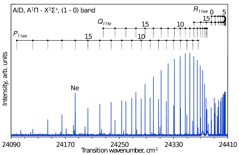
Figure 1: High-resolution FT-VIS emission spectrum of the AlD, ${A}\,^{1}\Pi-{X}\,^{1}\Sigma^{+}$ (1-0) band recorded with SNR of about $200:1$ and FWHM of lines about $0.08$ cm^-1. Bands of the $1-v^{\prime\prime}$ progression are observed up to the $J^{\prime}_{\max}=19$ lines due to the predissociation in the ${A}\,^{1}\Pi$ $(v=1)$ level.

3 MARVEL procedures

All currently available experimental transition frequencies (both extracted from literature and as part of this work) for AlH and AlD were analysed using the “Measured Active Rotational-Vibrational Energy Levels” (MARVEL) algorithm (Furtenbacher et al., 2007; Császár et al., 2007; Furtenbacher & Császár, 2012; Tóbiás et al., 2019). This algorithm consists of inverting a set of transition frequencies with their respective uncertainties into a consistent set of energy levels with the uncertainties propagated from all relevant transitions.

The AlH and AlD experimental data extracted is primarily concentrated around the first two singlet states ${X}\,^{1}\Sigma^{+}$, ${A}\,^{1}\Pi$ and their respective $X\,{}^{1}\Sigma^{+}$–$X\,{}^{1}\Sigma^{+}$ and $X\,{}^{1}\Sigma^{+}$–$A\,{}^{1}\Pi$ bands. The work description of the sources is divided between AlH and AlD.

3.1 AlH

Many of the sources used in this work for AlH have been previously discussed by Yurchenko et al. (2018b); Szajna & Zachwieja (2009) and Voronina & Voronin (2019), with the addition of a few older papers not used in our previous MARVEL study. The quantitative description of the data used in MARVEL from the sources can be seen in Table 1. The qualitative descriptions of the sources for AlH denoted by their MARVEL tags are as follows:

23YuSzHa_astro (Current work): as part of the current work 79 rovibronic transitions of AlH in the ${A}\,^{1}\Pi-{X}\,^{1}\Sigma^{+}$ system are reported in the current work as part of a reanalysis of the stellar (Proxima Cen) spectra from the HARPS ESO public data archive (Mayor et al., 2003), for the (0–0), (1–0), (1–1) bands (see below). The transition data is included as part of the MARVEL input data and can be seen separately in the Table 12 of the Appendix.

23SzKePa: Szajna et al. (2023) reported FT-VIS emission spectra of AlH with 259 transitions in the $A\,{}^{1}\Pi$–$X\,{}^{1}\Sigma^{+}$ system for the (0–0), (0–1),(0–2), (1–0), (1–1), (1–2), (1–3), (1–4) bands.

22PaTeYu: Pavlenko et al. (2022) reported 133 rovibronic transitions of AlH from their stellar (Proxima Cen) spectra in the $A\,{}^{1}\Pi$–$X\,{}^{1}\Sigma^{+}$ system for the (0-0), (0-1), (1-0), (1-1), (1-2) bands. The transitions were predominantly reported as $\lambda_{\rm air}$ in Å and had to be converted to $\nu_{\rm vacuum}$ in cm^-1 for consistency. This was done using the method described in Ryabchikova et al. (2015) and attributed to N. Piskunov.

16HaZi: Halfen & Ziurys (2016) reported hyperfine rotational transitions of AlH between $J=2\leftarrow 1$ in the $X\,{}^{1}\Sigma^{+}$ state measured using the terahertz direct absorption spectroscopy. The pure rotational frequency from this work was calculated using the common expression for the total hyperfine energy (Gee & Wasylishen, 2001; Gordy & Cook, 1984) as a sum of the electric quadrupole and nuclear spin-rotation terms for ${}^{27}\text{Al}$. The weighted average values of the hyperfine corrected pure rotational frequency of the $R(1)$ line is $755,211.403(90)$ MHz. The methodology use to calculated pure rotational frequency is described in further detail in Appendix B.

14HaZi: Halfen & Ziurys (2014) reported hyperfine rotational transitions of AlH between $J=2\leftarrow 1$ in the $X\,{}^{1}\Sigma^{+}$ state measured using the terahertz direct absorption spectroscopy. The pure rotational transition value from this work data is $R(1)=755,198.117(87)$ MHz (see method description in 16HaZi and Appendix).

11SzZaHa: Szajna et al. (2011) reported 47 AlH emission transitions from the $A\,{}^{1}\Pi$–$X\,{}^{1}\Sigma^{+}$ system and the (0-2) band.

09SzZa: Szajna & Zachwieja (2009) reported emission spectra of AlH with 183 transitions in the $A\,{}^{1}\Pi$–$X\,{}^{1}\Sigma^{+}$ system for the (0-0), (0-1), (1-0), (1-1), (1-2), (1-3) bands. A local minor perturbation in the $A\,{}^{1}\Pi$ $v^{\prime}=1$, $J^{\prime}=5$ was reported and attributed to the a ${}^{3}\Pi$ state.

04HaZi: Halfen & Ziurys (2004) reported hyperfine rotational transitions in AlH between $J^{\prime}=1$ and $J^{\prime\prime}=0$ in the $X\,{}^{1}\Sigma^{+}$ state measured using submillimeter direct absorption spectroscopy. The pure rotational transition value from this work data is $R(0)=377,737.022(90)$ MHz (see method description in 16HaZi).

96RaBe: Ram & Bernath (1996) reported emission spectra of AlH with 66 rovibronic transitions in the $A\,{}^{1}\Pi$–$X\,{}^{1}\Sigma^{+}$ system for the (0-0), (1-1) bands.

95GoSa: Goto & Saito (1995) reported hyperfine rotational transitions in AlH between $J^{\prime}=1$ and $J^{\prime\prime}=0$ in the $X\,{}^{1}\Sigma^{+}$ state measured using the submillimeter-wave spectrometer. The pure rotational transition value from this work data is $R(0)=377,738.10(72)$ MHz (see method description in 16HaZi).

94ItNaTa: (Ito et al., 1994) reported Fourier Transform Infrared (FTIR) absorption spectra of AlH with 87 rovibrational transitions in the $X\,{}^{1}\Sigma^{+}$–$X\,{}^{1}\Sigma^{+}$ system for the (1-0), (2-1), (3-2), (4-3) bands.

93WhDuBe: White et al. (1993) reported FTIR emission spectra of AlH with 260 rovibrational transitions observed in the $X\,{}^{1}\Sigma^{+}$–$X\,{}^{1}\Sigma^{+}$ system for the (1-0), (2-1), (3-2), (4-3), (5-4) bands.

92YaHi: Yamada & Hirota (1992) reported infrared diode laser absorption spectra with 22 rovibrational transitions in the $X\,{}^{1}\Sigma^{+}$–$X\,{}^{1}\Sigma^{+}$ system for the (1-0), (2-1), (3-2), (4-3) bands.

87DeNeRa: Deutsch et al. (1987) reported emission spectra of AlH with 333 rovibrational transitions in the $X\,{}^{1}\Sigma^{+}$–$X\,{}^{1}\Sigma^{+}$ system with the $\Delta v=2$ sequence for the (2-0), (3-1), (4-2), (5-3), (6-4), (7-5), (8-6) bands.

54ZeRi: Zeeman & Ritter (1954) reported both emission and absorption bands of AlH with 162 rovibronic transitions observed in the $A\,{}^{1}\Pi$–$X\,{}^{1}\Sigma^{+}$ system for the (0-2), (0-3), (1-3), (1-4) bands.

34Holst: (Holst, 1934) reported an absorption band with 25 rovibronic transitions for the AlH as a ${}^{1}\Sigma^{***}$–${}^{1}\Pi$ system. Through matching with the newer experiments this band was identified as (0-2) of the $A\,{}^{1}\Pi$–$X\,{}^{1}\Sigma^{+}$ system.

30BeRy: Bengtsson & Rydberg (1930) reported two emission bands with 76 rovibronic transitions for the AlH as a ${}^{1}\Pi$ $\rightarrow$ ${}^{1}\Sigma$ system. Through matching with the newer experiments these bands were identified as (0-1) and (1-2) of the $A\,{}^{1}\Pi$–$X\,{}^{1}\Sigma^{+}$ system.

A complete set of experimentally derived energy term values for the AlH represented in the rotational decomposition can be seen in Figure 2. The quantitative description of MARVEL-derived AlH term values can be found in Table 2.

Figure 2: Experimentally derived reduced energy term values for the AlH in the rotational decomposition.

Table 1: List of transition lines used in MARVEL procedure for AlH grouped by source.

Segment tag	Source	Range cm-1	A/V	MSU cm-1	LSU cm-1	ASU cm-1
23YuSzHa_astro	current work	22618.80 - 24583.50	79/79	1.600e-2	1.142e+0	1.165e-1
23SzKePa	Szajna et al. (2023)	18275.458 - 24585.496	259/259	2.000e-3	4.360e-2	4.209e-3
22PaTeYu	(Pavlenko et al., 2022)	22742.0 - 24556.1	24/24	1.000e-2	1.038e+0	1.443e-1
16HaZi	Halfen & Ziurys (2016)	25.1911 - 25.1911	1/1	2.681e-4	2.681e-4	2.681e-4
14HaZi	Halfen & Ziurys (2014)	25.1907 - 25.1907	1/1	3.729e-4	3.729e-4	3.729e-4
11SzZaHa	Szajna et al. (2011)	20067.602 - 20468.352	47/47	3.000e-3	1.958e-2	4.714e-3
09SzZa	Szajna & Zachwieja (2009)	19724.41 - 24585.49	183/183	3.000e-2	3.000e-2	3.000e-2
04HaZi	Halfen & Ziurys (2004)	12.59995 - 12.59995	1/1	2.643e-5	2.643e-5	2.643e-5
96RaBe	Ram & Bernath (1996)	22782.590 - 23572.451	66/66	3.000e-3	2.377e-2	4.619e-3
95GoSa	Goto & Saito (1995)	12.59999 - 12.59999	1/1	1.722e-5	1.722e-5	1.722e-5
93WhDuBe	White et al. (1993)	1225.5735 - 1802.7058	260/260	2.000e-4	5.953e-3	3.204e-4
94ItNaTa	Ito et al. (1994)	1400.4802 - 1793.1351	87/87	1.000e-4	2.300e-3	6.969e-4
92YaHi	Yamada & Hirota (1992)	1432.09 - 1781.54	22/22	3.000e-3	1.000e-1	1.129e-2
87DeNeRa	Deutsch et al. (1987)	2405.968 - 3292.072	333/329	3.000e-3	2.490e-1	7.084e-3
54ZeRi	Zeeman & Ritter (1954)	18195.18 - 20477.47	162/148	1.000e-2	1.810e-1	2.852e-2
34Holst	Holst (1934)	20034.93 - 20281.98	25/14	5.000e-2	1.855e-1	8.748e-2
30BeRy	Bengtsson & Rydberg (1930)	21226.3 - 21988.9	76/71	5.000e-1	4.348e+1	1.149e+0

A/V - Available lines vs Verified
MSU - Minimal uncertainty
LSU - Largest uncertainty
ASU - Average uncertainty

Table 2: Description of AlH energy levels derived from MARVEL.

State	$v$	$J$ Range	Unc. Range cm-1	Avg. of Unc. cm-1	Range of energy levels cm-1
$A\,{}^{1}\Pi$	0	1 - 24	0.0040 - 1.9836	0.1066	23482.94 – 26810.43
	1	0 - 13	0.0040 - 1.7813	0.1662	24553.99 – 25468.85
$X\,{}^{1}\Sigma^{+}$	0	0 - 33	0.0000 - 0.0663	0.0136	0.0000 – 6629.52
	1	0 - 34	0.0004 - 0.0659	0.0136	1625.07 – 8419.93
	2	0 - 35	0.0008 - 0.0663	0.0136	3194.21 – 10143.16
	3	0 - 36	0.0012 - 0.0667	0.0138	4708.82 – 11800.00
	4	0 - 35	0.0016 - 0.0654	0.0128	6170.19 – 12697.60
	5	1 - 33	0.0020 - 0.0495	0.0123	7590.40 – 13256.44
	6	4 - 32	0.0101 - 0.0486	0.0202	9042.94 – 14131.90
	7	3 - 28	0.0080 - 0.0555	0.0174	10307.65 – 14170.79
	8	7 - 23	0.0161 - 0.0546	0.0277	11781.03 – 14129.84

3.2 AlD

As for AlH, there have been previous discussions of the sources used in Yurchenko et al. (2018b); Szajna & Zachwieja (2009) and Voronina & Voronin (2019). The quantitative description of the data used in MARVEL from the sources can be seen in Table 3. The qualitative descriptions of the sources for AlD denoted by their MARVEL tags are as follows:

23YuSzHa (Current work): 491 rovibronic transitions of AlD in the ${A}\,^{1}\Pi-{X}\,^{1}\Sigma^{+}$ system are reported using the FT-VIS spectroscopy, as described in Section 2, for the (0-0), (0-1), (0-2), (1-0), (1-1), (1-2), (1-3), (1-4), (2-1), (2-2) bands. The full list of transitions can be found in Appendix (see Table 9 and 10).

22ShKaRa: Shanmugapriya et al. (2022) reported 76 rovibronic spectra transitions of AlD in the $A\,{}^{1}\Pi$–$X\,{}^{1}\Sigma^{+}$ for the (0-0), (1-2), (1-3) bands observerd in sunspot umbra. The MARVEL uncertainty was set to 0.1 cm^-1, the same as the tolerance of wavenumber reported for line identification in the sunspot spectra.

17SzMoLa: Szajna et al. (2017b) reported 379 rovibronic transitions of AlD in the $A\,{}^{1}\Pi$–$X\,{}^{1}\Sigma^{+}$ for the (0-0), (0-1), (1-0), (1-1), (1-2), (1-3) bands using the FT-VIS spectroscopy. The accuracy of the lines is assigned based on whether the line was distorted or not. Distorted lines had an accuracy of 0.01 cm^-1and clear lines were reported with uncertainty of 0.002 cm^-1.

17SzMoLa_hyperfine: Szajna et al. (2017b) also reported the pure rotational $R(1)=393661.660(36)$ MHz, $R(2)=590314.932(66)$ MHz and $R(3)=786755.135(122)$ MHz frequencies of the $X\,{}^{1}\Sigma^{+}$ $v=0$ provided by Halfen via private communication as calculated from their experimental data (Halfen & Ziurys, 2010, 2014).

15SzZaHa: Szajna et al. (2015) reported an emission spectrum of AlD with 133 rovibronic transitions in the $A\,{}^{1}\Pi$–$X\,{}^{1}\Sigma^{+}$ for the (0-0), (1-1) bands. Like 17SzMoLa, the accuracy reported depended on whether the lines were blended or not. Blended lines were reported with an accuracy of 0.005 cm^-1 and not blended with 0.003 cm^-1.

14HaZi: Halfen & Ziurys (2014) reported hyperfine rotational transitions of AlD between $J=4\leftarrow 3$ in the $X\,{}^{1}\Sigma^{+}$  measured using the terahertz direct absorption spectroscopy. The pure rotational frequency from this work was calculated using the common expression for the total hyperfine energy (Gee & Wasylishen, 2001; Gordy & Cook, 1984) as a sum of the electric quadrupole and nuclear spin-rotation terms for ${}^{27}\text{Al}$. The weighted average value of the hyperfine corrected pure rotational frequency of the $R(3)$ line is $786,755.195(77)$ MHz. The pure rotational value calculation is described in further detail in Appendix B.

10HaZi: Halfen & Ziurys (2010) reported hyperfine rotational transitions in AlD between $J=2\leftarrow 1$ and $J=3\leftarrow 2$ using submillimeter direct absorption spectroscopy. Additionally, predictions for the $J=1\leftarrow 0$ and $J=4\leftarrow 3$ transitions of AlD have been made. The pure rotational transition values from this data are $R(2)=590,314.920(43)$ MHz and $R(1)=393,661.697(52)$ MHz (see method description in 14HaZi). Contaminated lines were excluded from the weighted average calculation.

04HaZi: Halfen & Ziurys (2004) reported hyperfine rotational transitions in AlD between $J=2\leftarrow 1$ using submillimeter direct absorption spectroscopy. The pure rotational transition value from this data is $R(1)=393,661.772(55)$ MHz (see method description in 14HaZi).

93WhDuBe: White et al. (1993) reported FTIR emission spectra of AlD with 465 rovibrational transitions observed in the $X\,{}^{1}\Sigma^{+}$–$X\,{}^{1}\Sigma^{+}$ system for the (1-0), (2-1), (3-2), (4-3), (5-4), (6-5), (7-6) bands.

92UrJo: Urban & Jones (1992) reported infrared spectra of AlD with 114 rovibrational transitions observed in the $X\,{}^{1}\Sigma^{+}$–$X\,{}^{1}\Sigma^{+}$ system for the (1-0), (2-1), (3-2), (4-3), (5-4), (6-5), (7-6) bands.

48Nilsson: Nilsson (1948) reported emission spectra of AlD with 240 rovibronic transitions observed in the $A\,{}^{1}\Pi$–$X\,{}^{1}\Sigma^{+}$ system for the (0-0), (0-1), (1-0), (1-1), (1-2), (1-3), (2-1), (2-2) bands. The uncertainties were not reported as part of the work; based on how close the values were to the more recent experiments the original minimum uncertainty was set at 0.3 cm^-1. Additionally, the R branch transition for $J=0$ in the (1-0) band is off by 20 cm^-1 and is excluded from the analysis.

The complete set of experimentally derived energy term values for the AlH represented in the rotational decomposition, can be seen in Figure 3. The quantitative description of MARVEL-derived AlD term values can be found in Table 4.

The MARVEL input, transtion files, and output, energy files, for both AlH and AlD are given in the supporting material.

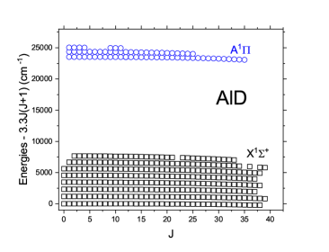
Figure 3: Experimentally derived reduced energy term values for the AlD in the rotational decomposition.

Table 3: List of transition lines used in MARVEL procedure for AlD grouped by source.

Segment tag	Source	Range cm-1	A/V	MSU cm-1	LSU cm-1	ASU cm-1
23YuSzHa	current work	19749.782 - 24406.512	491/491	2.000e-3	3.890e-2	5.589e-3
22ShKaRa	Shanmugapriya et al. (2022)	20805.3 - 23588.2	76/74	1.000e-1	1.000e-1	1.000e-1
17SzMoLa	Szajna et al. (2017b)	20755.112 - 24406.511	379/379	2.000e-3	2.133e-2	4.031e-3
17SzMoLa_hyperfine b	Szajna et al. (2017b)	13.131140 - 26.243326	3/3	1.201e-6	4.069e-6	2.491e-6
15SzZaHa	Szajna et al. (2015)	22945.366 - 23604.065	133/133	3.000e-3	2.307e-2	4.229e-3
14HaZi	Halfen & Ziurys (2014)	26.243328 - 26.243328	1/1	4.253e-6	4.253e-6	4.253e-6
10HaZi	Halfen & Ziurys (2010)	13.131141 - 19.690786	2/2	1.745e-6	1.945e-6	1.845e-6
04HaZi	Halfen & Ziurys (2004)	13.131143 - 13.131143	1/1	2.398e-6	2.398e-6	2.398e-6
93WhDuBe	White et al. (1993)	850.8496 - 1311.3449	465/465	2.000e-4	1.037e-2	3.540e-4
92UrJo	Urban & Jones (1992)	945.746 - 1193.703	114/114	5.000e-3	5.000e-3	5.000e-3
48Nilsson	Nilsson (1948)	20708.8 - 24406.4	240/215	2.000e-1	2.000e-1	2.000e-1

A/V - Available lines vs Verified
MSU - Minimal uncertainty
LSU - Largest uncertainty
ASU - Average uncertainty

Table 4: Description of AlD energy levels derived from MARVEL.

State	$v$	$J$ Range	Unc. Range cm-1	Avg. of Unc. cm-1	Range of energy levels cm-1
$A\,{}^{1}\Pi$	0	1 - 35	0.0044 - 0.4236	0.0783	23543.17 - 27229.71
	1	1 - 25	0.0040 - 0.4124	0.0963	24385.98 - 26175.82
	2	1 - 11	0.0064 - 0.4132	0.1473	25055.97 - 25381.24
$X\,{}^{1}\Sigma^{+}$	0	0 - 38	0.0000 - 0.0244	0.0134	0.00 - 4655.89
	1	0 - 39	0.0004 - 0.0248	0.0131	1181.94 - 5967.09
	2	0 - 37	0.0008 - 0.0236	0.0125	2334.58 - 6574.10
	3	0 - 38	0.0012 - 0.0240	0.0132	3458.43 - 7820.30
	4	0 - 37	0.0024 - 0.0236	0.0135	4554.01 - 8611.26
	5	0 - 38	0.0028 - 0.0240	0.0147	5621.82 - 9794.48
	6	1 - 39	0.0032 - 0.0276	0.0171	6668.10 - 10946.56
	7	2 - 33	0.0036 - 0.0349	0.0197	7692.91 - 10730.06

4 Spectroscopic model and refinement

We use the variational diatomic nuclear-motion code Duo (Yurchenko et al., 2016) to solve the coupled system of Schrödinger equations for a set of curves defining the spectroscopic model of the $X\,{}^{1}\Sigma^{+}$ and $A\,{}^{1}\Pi$ system of AlH and AlD. We used the Sinc DVR method for the vibrational degree of freedom on a grid of 1601 points ranging from 0.5 to 13.5 Å.

The AlH/AlD PEC in its the $A\,{}^{1}\Pi$ state has a shallow minimum with a small barrier to the dissociation, which can hold only two bound vibrational states in AlH ($v=0,1$) and three ($v=0,1,2$) in AlD as illustrated in Fig. 4. Furthermore, the highest vibrational states ($v=1$ and $v=2$, respectively) exhibit strong predissociative characters.

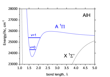
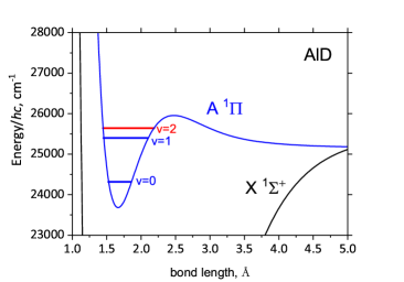
Figure 4: Refined potential energy curves of $X\,{}^{1}\Sigma^{+}$ and $A\,{}^{1}\Pi$ of AlH and AlD and the corresponding (quasi-)bound vibrational energy term values.

Following Yurchenko et al. (2018b), we use a diabatic representation to model the shallow $A\,{}^{1}\Pi$ PECs of AlH and AlD, with two diabatic PECs $V_{1}(r)$ and $V_{2}(r)$ coupled with a term $W(r)$ via a $2\times 2$ diabatic matrix

$$\bf{A}=\left(\begin{array}[]{cc}V_{1}(r)&W(r)\\ W(r)&V_{2}(r)\end{array}\right).$$ (1)

The functions $V_{1}(r)$, $V_{2}(r)$ and $W(r)$ are illustrated in Fig. 5 in the case of AlD. The diabatic PEC $V_{1}(r)$ is modelled with an EMO (Extended Morse Oscillator) function (Le Roy et al., 2006) as given by

$$V(r)=V_{\rm e}\;\;+\;\;(A_{\rm e}-V_{\rm e})\left[1\;\;-\;\;\exp\left(-\sum_{k=0}^{N}B_{k}\xi_{p}^{k}(r-r_{\rm e})\right)\right]^{2},$$ (2)

where $A_{\rm e}$ is a dissociation asymptote, $A_{\rm e}-V_{\rm e}$ is the dissociation energy, $r_{\rm e}$ is an equilibrium distance of the diabatic PEC, and $\xi_{p}$ is the Šurkus variable given by:

$$\xi_{p}=\frac{r^{p}-r^{p}_{\rm e}}{r^{p}+r^{p}_{\rm e}}.$$ (3)

$V_{2}(r)$ in Eq. (1) is modelled by a repulsive curve playing a role of a dummy state (called here $1\,{}^{1}\Pi$) and represented by:

$$V_{2}(r)=A_{\rm e}^{A}+\frac{a_{6}}{r^{6}},$$ (4)

with the asymptote $A_{\rm e}^{A}$ fixed to the dissociation asymptote of the $A\,{}^{1}\Pi$ state, $A_{\rm e}$ = 25500 cm^-1.

For the coupling function $W(r)$, an inverted EMO PEC with an asymptote of $W(r)\to 0$ at $r\to\infty$ was used

$$W(r)=W_{0}-W_{0}\left[1\;\;-\;\;\exp\left(-w_{0}(r-r_{0})\right)\right]^{2},$$ (5)

where $W_{0}$ is the height of the coupling at $r_{0}$, see Fig. 5.

The adiabatic PEC of $A\,{}^{1}\Pi$ is then given by the lower eigenvalue of the diabatic matrix $\bf{A}$ in Eq. (1) as

$$V_{A\,^{1}\Pi}(r)=\frac{V_{1}(r)+V_{2}(r)}{2}-\frac{\sqrt{[V_{1}(r)-V_{2}(r)]^{2}+4\,W^{2}(r)}}{2}.$$ (6)

The upper diabatic component is disregarded in the rest of the calculations.

The expansion parameters defining the diabatic curves were obtained in the fit to the MARVEL energies of AlH/AlD and are given in the supplementary material (see also below).

We used the EMO function to represent the PEC of the $X\,{}^{1}\Sigma^{+}$ state with the corresponding expansion parameters taken from and constrained to the values of Yurchenko et al. (2018b). A Born-Oppenheimer Breakdown (BOB) correction curve was added and modelled using the following function:

$$F(r)=\sum^{N}_{k=0}B_{k}\,z^{k}(1-\xi_{p})+\xi_{p}\,B_{\infty},$$ (7)

where $z$ is taken as a damped-coordinate given by

$$z=(r-r_{\rm ref})\,e^{-\beta_{2}(r-r_{\rm ref})^{2}-\beta_{4}(r-r_{\rm ref})^{4}},$$ (8)

see also Prajapat et al. (2017) and Yurchenko et al. (2018a). Here $r_{\rm ref}$ is a reference position equal to $r_{\rm e}$ by default and $\beta_{2}$ and $\beta_{4}$ are damping factors. In order to model the deviation of PEC of AlD from the AlH PEC, a diabatic correction term $\Delta V(r)$ was added to the adiabatic PEC $V_{A\,^{1}\Pi}(r)$, which was modelled with the same form as in Eq. (7).

A $\Lambda$-doubling empirical curve $q(r)$ was also included in the fit modelled using Eq. (7) with a single expansion term

$$q(r)=q_{0}(1-\xi_{p})+\xi_{p}\,q_{\infty},$$

where $\xi_{p}$ as in Eq. (3).

The AlD PEC has an extra vibrational state, $v=2$ (see Fig. 4), which samples a larger range of the PEC than that of AlH. We, therefore, decided to process the AlD curves first by fitting to the experimentally derived (MARVEL) energies, and then refine the AlD spectroscopic model for AlH by fitting to the corresponding MARVEL energies (see above).

Because of the limited amount of experimental data and high complexity of the diabatic model, the fit is highly degenerate. As a work around we applied a rather subjective criterion of physically sensible shapes of the diabatic curves. During this user-guided fit, attention was paid to the predissociative lifetimes of the $A\,{}^{1}\Pi$ $v=2$ states of AlD and $v=1$ states of AlH, which had to be consistent with the experimental data: predissociative line shapes as in Pavlenko et al. (2022) as well as lifetimes (see discussion below).

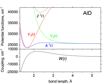
Figure 5: Adiabatic PECs of $A\,{}^{1}\Pi$  (blue dashed curve) and $2~{}^{1}\Pi$ (black dash) of AlD and the corresponding curves in the diabatic representation, PECs $V_{1}(r)$ (red) and $V_{2}(r)$ (green) and the diabatic coupling curve $W(r)$ (lower display).

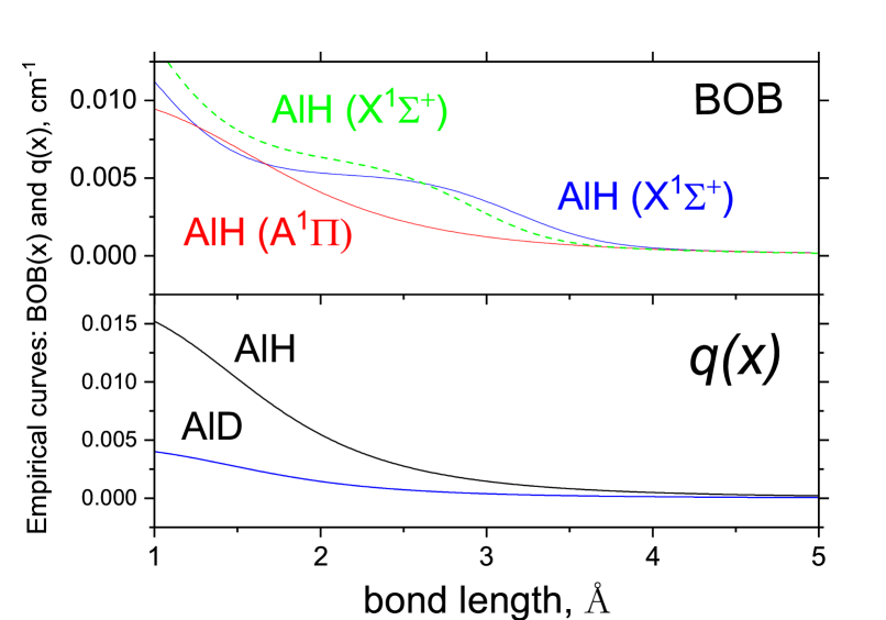
Figure 6: Curves for AlH and AlD: Upper panel, Born-Oppenheimer breakdown (BOB); lower panel, $\Lambda$ doubling, $q(r)$ .

The final spectroscopic model of AlD consists of 14 varying parameters reproducing the AlD 423 MARVEL energies with the root-mean-square (rms) error of 0.06 cm^-1. The corresponding curves are illustrated in Figs. 4 and 6. The residuals are shown in Fig. 7.

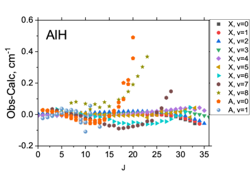
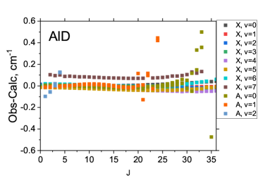
Figure 7: Obs.-calc. residuals between the MARVEL and calculated energies of AlH and AlD using the corresponding refined models.

In the AlH fit, the $A\,{}^{1}\Pi$ PEC was constrained to that of AlD. In order to allow for variation in the shapes of the corresponding curves, an ‘adiabatic’ potential correction term was added to the model using Eq. (7). We also introduced a BOB term for $A\,{}^{1}\Pi$ of AlH and varied the parameter $q_{0}$ of the $\Lambda$-doubling curve $q(x)$. The $X\,{}^{1}\Sigma^{+}$ PEC parameters were still constrained to the values from Yurchenko et al. (2018b), but we refitted the $X\,{}^{1}\Sigma^{+}$ BOB term to improve the quality of the model. The AlH spectroscopic model consists of 8 parameters reproducing 346 MARVEL energies (see above) with an rms error of 0.08 cm^-1.

The dipole moment and transition dipole moment curves were taken from Yurchenko et al. (2018b).

All curves or parameters defining the AlH and AlD spectroscopic models are given as part of the supplementary material to the paper in the form of Duo input files.

4.1 Lifetimes and predissociation line broadening

As part of the ExoMol States files, the lifetimes of species are usually included (see Table 6). In most cases of negligible predissociation effects, the radiative lifetime (of a state $i$) is computed via

$$\tau_{i}^{\rm rad}=\frac{1}{\sum_{j<i}A_{ij}},$$ (9)

where $A_{ij}$ are the Einstein $A$ coefficients for all states $j$ lower than $i$. According to the recent changes to the ExoMol format (Tennyson et al., 2023), predissociative lifetimes $\tau_{\rm prediss}$ are to be included into the line list with the radiative lifetimes, if non-negligible, which is the case for many $A\,{}^{1}\Pi$ rovibronic states of AlH and AlD. Here we used the LEVEL program (Le Roy, 2017) to estimate lifetimes for the predissociative $A\,{}^{1}\Pi$ states of AlH ($v=1$) and AlD ($v=2$) with the our new PECs. LEVEL uses the uniform semiclassical procedure of Connor & Smith (1981) to compute the widths $\gamma$ (cm^-1) of the predissociative states, which we converted to lifetimes via

$$\tau_{\rm prediss}=\frac{1}{2\pi c\gamma_{\rm prediss}},$$ (10)

where $c$ is the speed of light in cm s^-1. These are shown in Table 5; our lifetimes show reasonable agreement with the laboratory values obtained by Baltayan & Nedelec (1979) using in a hollow cathode discharge by dye laser excitation as well as the astrophysical estimates of (Pavlenko et al., 2022) from analysis of Proxima Cen predissociative spectrum of AlH. The LEVEL predissociative values $\tau_{\rm prediss}$ are then added to the radiative lifetime to give total lifetime in the States file:

$$\frac{1}{\tau_{\rm total}}=\frac{1}{\tau_{\rm rad}}+\frac{1}{\tau_{\rm prediss}}.$$ (11)

The lifetimes can be then used to evaluate the line broadening of the the predissociated lines by inverting Eq. (10) for the HWHM $\gamma_{\rm prediss}$ and apply alone side the collisional value of $\gamma_{\rm col}$:

$$\gamma_{\rm total}\approx\gamma_{\rm col}+\gamma_{\rm prediss}.$$ (12)

This feature is now implemented in the spectrum simulator ExoCross (Yurchenko et al., 2018c; Zhang et al., 2023).

Table 5: Lifetimes (pico second) of AlH and AlD in their $A\,{}^{1}\Pi$ state: $\tau_{\rm rad}$, $\tau_{\rm prediss}$, by 79BaNe (Baltayan & Nedelec, 1979) and 22PaTeYu (Pavlenko et al., 2022).

$v$	$J$	$\tau_{\rm rad}$	$\tau_{\rm prediss}$	79BaNe	22PaTeYu		$v$	$J$	$\tau_{\rm rad}$	$\tau_{\rm prediss}$
AlH							AlD
0	17	88770	339418.03				2	1	130610	5044.98
0	18	91120	11817.11				2	2	131170	3649.69
0	19	94209	786.81				2	3	131870	2295.71
0	20	97872	85.74				2	4	132920	1284.75
0	21	130660	14.05	9.9	10($\frac{+10}{-5}$)		2	5	134310	656.50
0	22	347810	3.24				2	6	136450	314.52
0	23	166570	0.99	0.92	0.63($\frac{+0.26}{-0.18}$)		2	7	138430	144.85
0	24	268810	0.39	0.45	0.32 $\pm 0.07$		2	8	160270	65.56
0	25		0.18				2	9	168650	29.73
0	26		0.10				2	10	167640	13.72
1	6	113580	375687.32				2	11	168570	6.53
1	7	115640	26541.53				2	12	217830	3.25
1	8	118230	2651.90				2	13	303440	1.74
1	9	121560	342.35				2	14	362560	0.76
1	10	126400	55.23				2	15	581010	0.46
1	11	148800	11.09				2	16		0.25
1	12	159980	2.80				2	17		0.15
1	13	228510	0.89
1	14	508120	0.35
1	15		0.16
1	16		0.09

5 Line Lists

Using the new empirical spectroscopic models of AlH and AlD, line lists AloHa for the $X\,{}^{1}\Sigma^{+}$, $A\,{}^{1}\Pi$ system were computed with Duo. In intensity calculations, we distinguish bound-to-bound and bound-to-free transitions and compute two line lists, bound-bound and continuum (bound-free). The transitions to the quasi-bound states, especially important in the $A\,{}^{1}\Pi$-$X\,{}^{1}\Sigma^{+}$ band, are included in the bound-bound line list. In order to improve the resolution of the continuum spectrum, we use a significantly larger calculation box, with the bond length ranging from 0.5 to 60 Å. Since Duo is a pure bound state variational method, it produces both (quasi-)bound and continuum eigenfunctions $\psi_{\lambda}(r)$ as part of the same variational calculations. All eigenfunctions are ortho-normal, including the continuum ones, and all satisfy the boundary conditions that they vanish exactly, together with their first derivatives, at both edges of the box.

In order to identify continuum states and then separate them from the (quasi-)bound states, we check if they have non-zero density across a region $\Delta r$ adjacent to the outer border $r_{\rm max}$ against some threshold value $\epsilon_{\rm max}$ as given by (see Yurchenko et al. (2023)):

$$\epsilon=\int_{r_{\rm max-\Delta r}}^{r_{\rm max}}|\psi_{\lambda}(r)|^{2}dr>\epsilon_{\rm max},$$ (13)

where the value of $\epsilon_{\rm max}$ must be tuned to the specific case. For the box size $L$ of 59.5 Å, the integration region was chosen as 40 Å. Figure 8 shows examples of reduced radial densities for the bound state $A\,{}^{1}\Pi$, $v=0$, $J=9$ and two quasi-bound states $A\,{}^{1}\Pi$, $v=1$, $J=9$ and $J=12$ together with an integration box used. The corresponding values of integrated densities $\epsilon$ are 0, $2.4\times 10^{-4}$ and $4.8\times 10^{-2}$, respectively and of the average densities $\epsilon/L$ of 0, $3.7\times 10^{-6}$Å^-1 and $7.8\times 10^{-4}$/Å^-1. Here we adopted the threshold value of $\epsilon=0.46$, which was tuned to allow the $J=25$, $v=1$, $A\,{}^{1}\Pi$ state, the highest $J$ observed for $A\,{}^{1}\Pi$ $v=1$ (Bengtsson & Rydberg, 1930), to be included in the AlH line list.

According to the new ExoMol data structure (Tennyson et al., 2023), bound and quasi-bound states and the corresponding Einstein $A$ coefficients ($X$–$X$, $X$–$A$) are stored in the bound ExoMol line lists, while continuum $A\,{}^{1}\Pi$ ‘states’ and the corresponding bound-free transitions to/from the bound $X\,{}^{1}\Sigma^{+}$ states form temperature-dependent photo-absorption cross sections, see also Pezzella et al. (2022).

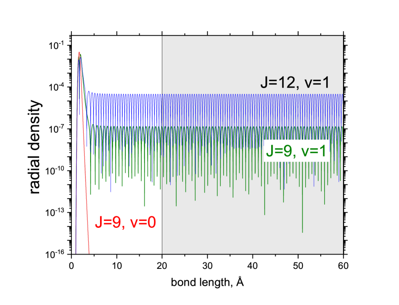
Figure 8: Reduced densities of AlH $\rho(r)$ for $J=9$ ($v=0$), $J=9$ ($v=1$) and $J=12$ ($v=1$) together with an integration box used to disentangle (quasi-)bound and continuum states.

5.1 (Quasi-)bound line lists of AlH/AlD

A bound ExoMol line list consists of a States file, Transition file and Partition function file computed using bound and quasi-bound wavefunctions. The AlH/AlD line lists cover the wavenumber range up to 30 000 cm^-1 ($<0.3333$ $\mu$m), $J=0\ldots 60$ of the $X\,{}^{1}\Sigma^{+}$ state, $J_{\rm max}=25$ ($A\,{}^{1}\Pi$) of AlH $A\,{}^{1}\Pi$  and $J_{\rm max}=36$ ($A\,{}^{1}\Pi$) of AlD. The vibrational excitations of the $X\,{}^{1}\Sigma^{+}$ are limited to $v=22$ for both AlH and AlD, which is just below the AlH dissociation limit, while for the $A\,{}^{1}\Pi$ state these are $v_{\rm max}=1$ (AlH) and $v_{\rm max}=2$ (AlD).

A States file (see an extract in Table 6) consists of state IDs, energy term values (cm^-1), total degeneracies, quantum numbers, energy uncertainties (cm^-1) and lifetimes (s^-1). The calculated energies are replaced with the MARVEL values where available. The uncertainties are taken as the MARVEL uncertainties for the substituted values. Otherwise, we use the following empirical and rather conservative expression as an estimate for uncertainties of the calculated energies:

$${\rm unc.}=\left\{\begin{array}[]{cc}0.01\,v+0.008\,v^{2}+0.0002\,J(J+1),&X\\ 0.05\,v+0.008\,v^{2}+0.002\,J(J+1),&A\end{array}\right.$$

The Transition files (see an extract in Table 7) consists of the IDs of the upper $f$ and lower $i$ states and Einstein $A_{fi}$ coefficients. The latter are the calculated values, i.e. not modified using the MARVEL energies and are given as reference only. We always recommend using energies from the State file for any practical purposes.

The partition function of AlH has been recomputed with the new line list but is very close to the one computed using the WYLLoT line list. This is unsurprising as the main contribution to the partition function is from the ground electronic state, and we, therefore, do not expect any significant changes from the current model of AlH. As before the partition function agrees well with the ones derived by Sauval & Tatum (1984) and Barklem & Collet (2016).

As a part of the AloHa data set, a set of bound-free temperature-dependent photo-absorption cross sections of AlH and AlD are provided. The cross sections are generated on a wavenumber grid of 0.01 cm^-1 ranging from 0 to 30 000 cm^-1 for a set of 50 temperatures, 100 K, 200 K, …, 5000 K. The AlH cross sections should be considered as add-ons for the spectra produced using the bound-bound line lists of AlH, see Tennyson et al. (2023).

A line list and photo-absorption data for the minor isotopologue ²⁶AlH was also produced using the ²⁷AlH spectroscopic model and the same calculation parameters but for a different mass of Al. ²⁶Al is radioactive with a half-life of about 710 000 years and has been clearly detected in the Milky Way (Diehl et al., 2006). We are not aware of any experimental data on the spectroscopy of²⁶AlH.

Table 6: Extract from the states file of the line list for AlH .

$i$	$\tilde{E}$ (cm-1)	$g_{i}$	$J$	unc. (cm-1)	$\tau$ (s-1)	Parity		State	$v$	${\Lambda}$	${\Sigma}$	$\Omega$	Ma/Ca	$\tilde{E}$ (cm-1)
292	24124.935533	252	10	0.009064	7.9391E-08	-	f	A1Pi	0	-1	0	-1	Ma	24124.987854
293	25119.784093	252	10	0.318000	2.0419E-11	-	f	A1Pi	1	-1	0	-1	Ca	25119.784093
294	24253.846482	276	11	0.014672	8.0291E-08	+	f	A1Pi	0	1	0	1	Ma	24253.897241
295	25228.674665	276	11	0.025744	5.9852E-12	+	f	A1Pi	1	1	0	1	Ma	25228.646969
296	825.362379	276	11	0.010672	2.6026E+01	-	e	X1Sigma+	0	0	0	0	Ma	825.362457
297	2426.330942	276	11	0.005744	4.9291E-03	-	e	X1Sigma+	1	0	0	0	Ma	2426.334029
298	3971.846039	276	11	0.010172	2.6279E-03	-	e	X1Sigma+	2	0	0	0	Ma	3971.835720
299	5463.280105	276	11	0.005910	1.8702E-03	-	e	X1Sigma+	3	0	0	0	Ma	5463.284608
300	6901.924290	276	11	0.010172	1.4991E-03	-	e	X1Sigma+	4	0	0	0	Ma	6901.933377
301	8288.978591	276	11	0.005916	1.2831E-03	-	e	X1Sigma+	5	0	0	0	Ma	8288.975579

$i$: State counting number.

$\tilde{E}$: State energy term values in cm^-1, MARVEL or Calculated (Duo).

$g_{i}$: Total statistical weight, equal to ${g_{\rm ns}(2J+1)}$.

$J$: Total angular momentum.

unc: Uncertainty, cm^-1.

$\tau$: Lifetime (s^-1).

$+/-$: Total parity; e/f: rotationless parity.

State: Electronic state.

$v$: State vibrational quantum number.

$\Lambda$: Projection of the electronic angular momentum.

$\Sigma$: Projection of the electronic spin.

$\Omega$: Projection of the total angular momentum, $\Omega=\Lambda+\Sigma$.

Label: ‘Ma’ is for MARVEL and ‘Ca’ is for Calculated.

$\tilde{E}$: State energy term values in cm^-1, Calculated (Duo).

Table 7: Extract from the transitions file of the line list for AlH.

$f$	$i$	$A_{fi}$ (s-1)
416	424	2.9549E+04
391	395	2.8823E+04
362	370	2.8164E+04
883	861	1.8092E+05
998	953	1.9332E-11
337	341	2.7560E+04
308	316	2.7001E+04
835	838	1.6168E+05
282	287	2.6475E+04

$f$: Upper state counting number;
$i$: Lower state counting number;
$A_{fi}$: Einstein-$A$ coefficient in s^-1.

5.2 Temperature-dependent photo-absorption cross sections of AlH/AlD

Using energies and Einstein coefficients from the bound ($X\,{}^{1}\Sigma^{+}$) and continuum ($A\,{}^{1}\Pi$) solutions, a set of temperature-dependent cross sections of AlH and AlD are computed, using a wavenumber grid of 0.01 cm^-1 and a temperature grid ranging from 100 K to 5000 K in steps of 100 K. Here we use the procedure established in Pezzella et al. (2021), where all discrete transition intensities to the continuum states are re-distributed in their vicinity to form continuum photo-absorption cross sections using a Gaussian line profile

$$f(\tilde{\nu})=\sqrt{\frac{\ln 2}{\pi}}\frac{1}{\alpha_{\rm G}}\exp\left(-\frac{(\tilde{\nu}-\tilde{\nu}_{fi})^{2}\ln 2}{\alpha_{\rm G}^{2}}\right),$$

where $\alpha_{\rm G}$ is the Gaussian half-width-at-half-maximum (HWHM). For the size box of $\sim$ 60 Å, the distance between the ‘continuum’ lines does not exceed 26 cm^-1, which adopt as the values of $\alpha_{\rm G}$.

Figure 9 shows the continuum (bound-unbound) spectrum of AlH at $T=1000$ K generated using the Gaussian profile smoothing with HWHM of 26 cm^-1. As an illustration, the original separation between the ‘unbound’ discrete absorption lines before the smoothing applied can be seen in the same spectrum generated using HWHM = 2 cm^-1.

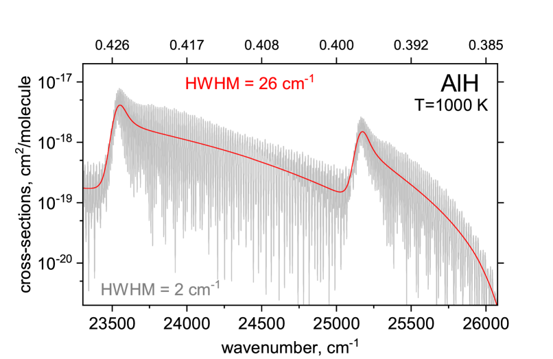
Figure 9: Example of the photo-absorption continuum cross sections of AlH at $T=1000$ K generated using a Gaussian line profile of HMWM = 26 cm^-1 (red line), overlaid with the same spectrum but using HMWM = 2 cm^-1 (grey line).

When computing the total cross sections of a molecule using the extended ExoMol format (Tennyson et al., 2023), we first compute cross sections for a given temperature and pressure using the (quasi-)bound line list and then add them to the photo-absorption cross section for the temperature in question. The pressure dependence of the continuum transitions is ignored.

Figure 10 (left) shows total (bound+continuum) cross sections of AlH for four temperatures and zero pressure computed using the procedure described above. In the same figure, where the 1000 K spectrum is also compared to the ab initio cross sections by Qin et al. (2021). Despitte a generally good agreement between the continuum contributions, our semi-empirical model provides more accurate data for high-resolution applications.

In Figure 11, we compare absorption spectra of AlH and AlD simulated using the WYLLoT and AloHa line lists at $T=1000$ K. The main differences are (i) the continuum contributions in the spectra and (ii) the $v^{\prime}=2$ bands in the spectrum of AlD, missing in the WYLLoT simulations.

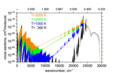
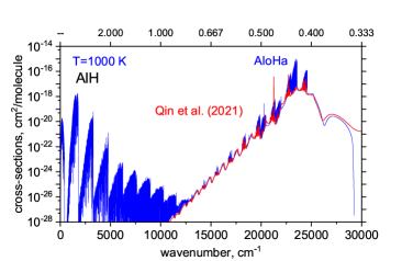
Figure 10: Temperature dependence of the AlH absorption spectrum using the Gaussian profile with HWHM = 1 cm^-1 (left) and a comparison with the $T=1000$ K cross-sections of AlH by Qin et al. (2021)

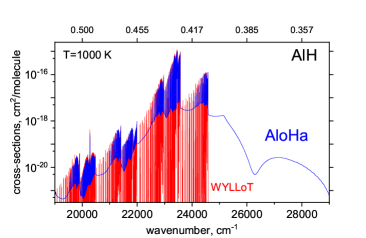
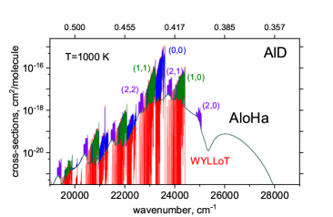
Figure 11: Comparison of the WYLLoT and AloHa simulations of $T=$ 1000 K absorption spectra of AlH (Left display) and AlD (Right display) using the Gaussian line profile with HWHM of 1 cm^-1.

5.3 Simulations of spectra of AlH and AlD

As illustrations, here we simulate emission spectra of AlH and AlD to compare to the experimental spectra from Szajna et al. (2023) and the current work, respectively. All spectra were generated using our open-access Fortran code ExoCross (Yurchenko et al., 2018c). Figure 12 shows a general overview of the AlH emission spectra generated using a Gaussian line profile with the HWHM of 0.08 cm^-1 and the rotational temperature of 750 K, where the vibrational temperature of $T_{\rm vib}=$ 4500 K was assumed as in Yurchenko et al. (2018b).

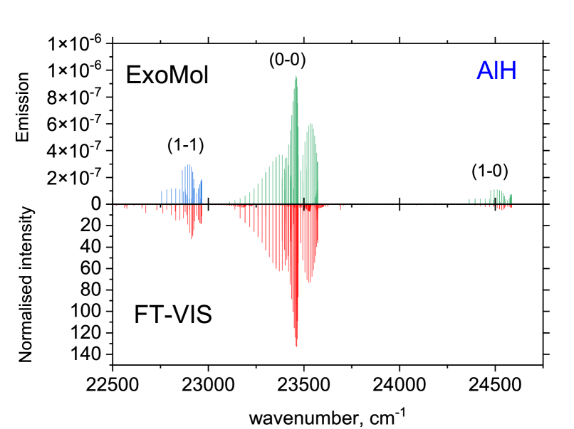
Figure 12: Comparison of the experimental FT-VIS by Szajna et al. (2023) and simulated AloHa  ${A}\,^{1}\Pi-{X}\,^{1}\Sigma^{+}$ spectrum of AlH in the region of the (1-1), (0-0) and (1-0) bands. For the theoretical spectrum, a rotational temperature of $T=750$ K and vibrational temperature $T=4500$ K were used; and a Gaussian line profile with FWHM of 0.08 cm^-1 was assumed

Figure 13 provide a similar illustration for AlD, where the simulations of the regions containing the (1-1), (0-0) and (1-0) bands are shown. The appearance of an extra line in the right display is due to the predissociative effects and discussed below.

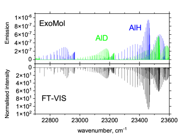
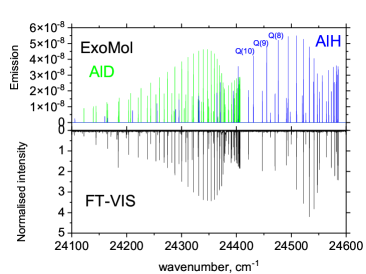
Figure 13: Comparison of the current experimental FT-VIS and simulated ExoMol ${A}\,^{1}\Pi-{X}\,^{1}\Sigma^{+}$ spectrum of AlD with AlH present: Left display, (1-1) and (0-0) bands, assuming AlH:AlD is 1:1. Right display, (1-0) band, AlH:AlD is 1:0.5. For the theoretical spectrum a rotational temperature of $T=750$ K and a Gaussian line profile with FWHM of 0.08 cm^-1 were assumed.

For the sake of completeness, we reproduce a comparison of the IR of AlH ($X\,{}^{1}\Sigma^{+}$–$X\,{}^{1}\Sigma^{+}$) with the emission measurements by White et al. (1993), see Yurchenko et al. (2018b). The current line list preserves the high quality of the original ExoMol line list WYLLoT.

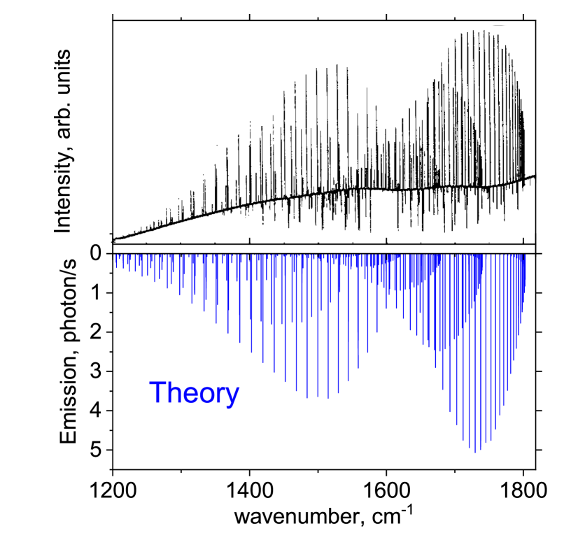
Figure 14: Infrared spectrum of AlH by White et al. (1993) (upper) compared to the emission spectrum computed using our line list assuming a temperature of 1700 K and a Gaussian profile with the FWHM of 0.01 cm^-1.

Pavlenko et al. (2022) recently studied the absorption of AlH in the spectrum of Proxima Cen from the HARPS ESO public data archive (Mayor et al., 2003), recorded over the spectral range from 3780 to 6810 Å with a resolving power $R\sim 115000$. This study has demonstrated the importance of the accurate description of line lists of AlH. In particular, the previous AlH line list WYLLoT was shown to deteriorate the higher $J$ spectral lines of AlH in the $v=0$ and $v=1$. It also could not describe the predissociative broadening effects in this band for $J>19$ in $v^{\prime}=0$ and $J>8$ in $v^{\prime}=1$. In Figs. 15 and 16 we simulate the high resolution AlH spectrum in model of stellar atmosphere appropriate for Proxima Cen in the spectral region covering (1-0), (0-0) and (1-1) bands of A${}^{1}\Pi$ – X${}^{1}\Sigma^{+}$ system. For details of the calculations please consult Pavlenko et al. (2022). To underline the prominent presence of AlH molecular lines in the spectrum one of the two synthetic spectra (the red one) includes only molecular lines. Fig. 15 shows (0-0) band and Fig. 15 presents bands which upper level is $v^{\prime}=1$ - the first two panels show the (1-0) band and the next two panels show (1-1) band. The actual list of lines of AlH shows very good consistency with the observed spectrum both in line position and in profiles of diffusive lines. Some differences in line shapes and in depths of broad atomic lines and of diffusive molecular lines may be ascribed to the uncertainty in the continuum tracing of the observed spectrum before its normalization. Simulations show a much better description of the AlH spectrum in Proxima Cen, including the predissociative broadening effects. Even the heavily predissociated lines $Q(13)$, $Q(14)$, $Q(15)$ of $v^{\prime}=1$ and $Q(23)$ and $Q(24)$ of $v^{\prime}=0$ can be clearly recognised. The presence of $Q(25)$ (See the bottom panel of Fig. 15) is less evident in the observed spectrum. The approach used to model the predissociation line broadening is described in details in Section 4.1.

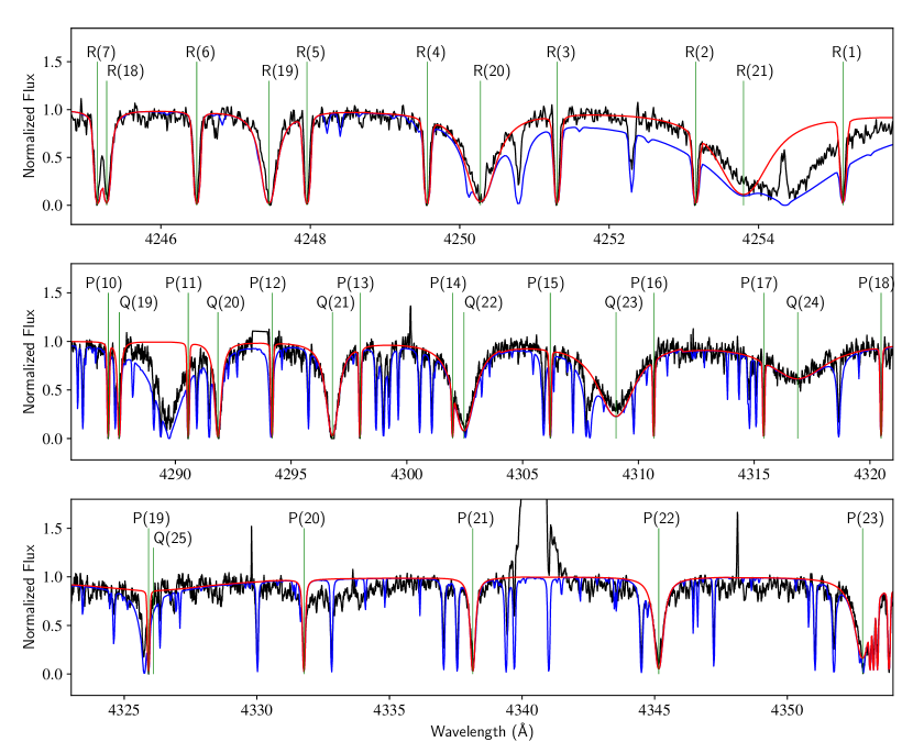
Figure 15: Comparison with the observed spectrum of AlH of Proxima Cen analysed by Pavlenko et al. (2022) shown by black line for the (0-0) band spectral range. Here and onward, we have adhered to the procedure of computation and identification of spectral features outlined by Pavlenko et al. (2022). The blue line marks the synthetic spectrum including atomic and molecular species, the red line spectrum is calculated including AlH lines only. A version of this figure, with the atomic lines also indicated, is provided in the Appendix, see 20.

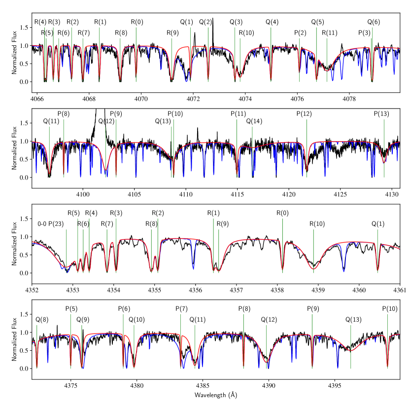
Figure 16: Comparison of the spectrum of AlH of Proxima Cen by Pavlenko et al. (2022) with the synthetic spectrum. Two upper panels show the spectral range of the 1-0 band and the two lower of the 1-1 band. The observed spectrum is shown by black line. The blue line marks the synthetic spectrum including atomic and molecular species, the red line spectrum is calculated including AlH lines only.

5.4 Breaking-off of predissociation lines of AlH and AlD

Figure 17 shows the experimental spectrum of the (2,2) band of AlD from this work and our attempt to model it using the new AloHa line list. Only the $J^{\prime}\leq 4$ lines appear in the experiment while the theory predicts lines with higher $J$. In fact, higher $J$ ($J\leq 11$) predissociative lines were observed experimentally by Nilsson (1948). The effect of “breaking-off” of the predissociative lines in different experimental setups was studied by Bengtsson & Rydberg (1930) and discussed by Herzberg (1939) and was attributed to the non-local thermal equilibrium (non-LTE) effects present in some low pressure conditions. In LTE, the number of predissociating molecules is compensated by new molecules formed by inverse predissociation.

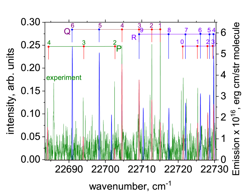
Figure 17: Comparison of the experimental FT-VIS and simulated ExoMol $A\,{}^{1}\Pi$-$X\,{}^{1}\Sigma^{+}$ (2-2) emission band of AlD. For the theoretical spectrum a rotational temperature of $T=750$ K and a Gaussian line profile with HWHM of 0.08 cm^-1 were assumed.

This effect can be nicely demonstrated in the comparison of the experimental FT spectrum of AlH from (Szajna et al., 2023) with our that of Proxima Cen as shown in Fig. 19. This figure reproduces our simulation of the Proxima Cen from the bottom display of Fig. 15 and the experimental spectrum is converted to air for a better comparison. It is evident how the emission lines from the FT spectrum break off for $J^{\prime}>8$ in comparison to the spectrum of Proxima Cen. It should be noted that this is not due to the lower temperature conditions of the FT spectrum. Indeed, if we assumed the LTE, the population of the corresponding states with $J\geq 8$ is comparable to those visible in the spectrum at $T=750$ K, indicating that the breaking-off of $J\geq 8$ in the experiment is due to non-LTE effects.

The effect can be also seen in right display of Fig. 13, where extra $Q(J)$ lines ($J>7$) of AlH appear compared to the experimental spectrum.

5.5 Collisional line-broadening parameters

Collisional line-broadening parameters of AlH for the $X\,{}^{1}\Sigma^{+}$ state with different partners (H₂, He, N₂, and AlH) have been computed using the MCRB approach (Antony et al., 2006). This is a semi-classical approach where internal degrees of freedom of the radiator and the perturber are treated quantum-mechanically and their relative translational motion is described classically. Line broadening can be said to appear as a consequence of monochromatic wave-train interruption when the radiating molecule is interacting with a perturber during a collision. The magnitude of this effect for completed collisions is described with a scattering matrix, which in this approach is expanded up to the second order in perturbation theory (Hartmann et al., 2008). The model interaction potential between the radiator (AlH) and a perturber is constructed from short-ranged and long-ranged parts. The former, repulsive part is obtained from atom-atom Lennard-Jones contributions (Svehla, 1962), while the latter is composed from electrostatic interactions and uses molecular multipole moments from NIST (Johnson, 2022). Trajectories are computed within the rigid rotor approximation using equilibrium geometries of the $X\,{}^{1}\Sigma^{+}$ state and a different isotropic potential to drive them (Loukhovitski & Sharipov, 2021).

Vibrational dependence of broadening parameters have also been modelled, assuming that only the changes in long-ranged van-der-Waals interactions with vibrational state significantly change scattering cross-sections. Diagonal rovibrational matrix elements of the $X\,{}^{1}\Sigma^{+}$ electric dipole moment $\langle vJ\!\mid\!\!\mu^{2}(r)\!\!\mid\!vJ\rangle$ and isotropic polarizability $\langle vJ\mid\!\alpha_{\text{iso}}(r)\!\mid vJ\rangle$ curves required for this part were computed using Duo’s ro-vibrational wavefunctions $|vJ\rangle$. The polarizability curve $\alpha_{\text{iso}}(r)$ was computed ab initio with MOLPRO (Werner et al., 2020) using the CCSD(T)/aug-cc-pVQZ level of theory as second order derivatives of the $X\,{}^{1}\Sigma^{+}$ energy with respect to the electric field. It is shown in Fig. 18. The dipole moment curve of $X\,{}^{1}\Sigma^{+}$ was taken from Yurchenko et al. (2018b).

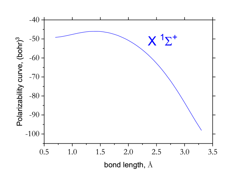
Figure 18: Ab initio isotropic electric polarizability curve of AlH.

It is worth mentioning that this semi-classical approach works best when the interaction potential is fitted to improve agreement with experimental broadening coefficients. Without this adjustment, theoretical values usually overestimate experimental ones (Ma et al., 2013). However, to the best of our knowledge, no experimental measurements of AlH broadening by any molecules are available, so our broadening coefficients are presented without any adjustments.

The new broadening parameters of AlH are included into the ExoMol database using the ExoMol diet format (Barton et al., 2017), which is based on the representation of the temperature- and pressure-dependence of the half-width-at-half-maximum $\gamma$ (cm^-1/atm) by a single-power law:

$$\gamma(T,P)=\gamma_{0}\left(\frac{T_{\rm ref}}{T}\right)^{n}\frac{P}{P_{\rm ref}},$$ (14)

where $T_{\rm ref}$ is the HITRAN reference temperature of 296 K and $P_{\rm ref}$ is the reference pressure of 1 atm. The $J$-dependence is best parameterised by the standard HITRAN $\mid\!\!m\!\!\mid$ dependence , where $m=J_{\text{lower}}+1$ for the R-branch and $m=-J_{\text{lower}}$ for the P-branch. We have therefore introduced a new ExoMol diet type $m0$. An example of the the diet file for AlH broadened by H₂ is given in Table 8. Our MCRB calculations predict a mildly sloping dependence on $m$ (and therefore $J$). The m0 type is implemented and now available in ExoCross.

The methodology described is currently only applicable to the ground $X\,{}^{1}\Sigma^{+}$ electronic state rovibrational transitions. The production of line shape parameters for rovibronic transitions is more complicated, see Buldyreva et al. (2024), and will be considered separately.

Table 8: ExoMole diet line broadening file for AlH with H₂ as perturber.

Type	$\gamma_{0}$	$n$	$m$
m0	0.1482	0.6179	1
m0	0.1462	0.6107	2
m0	0.1443	0.6040	3
m0	0.1420	0.5962	4
m0	0.1401	0.5903	5
m0	0.1386	0.5862	6
m0	0.1375	0.5837	7
m0	0.1367	0.5825	8
m0	0.1362	0.5824	9
m0	0.1360	0.5833	10
m0	0.1360	0.5851	11
m0	0.1362	0.5876	12
m0	0.1365	0.5904	13

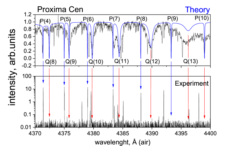
Figure 19: Comparison of the experimental FT-VIS (Szajna et al., 2023) of AlH (bottom) and the Proxima Cen spectrum (top), observation and simulation ($T=2900$ K) in the region of $A\,{}^{1}\Pi$-$X\,{}^{1}\Sigma^{+}$ (1-1) band using the new ExoMol line list as in the bottom display of Fig. 15. The blue/red arrows indicate the AlH lines that are present/disappear in the experiment.

6 Conclusions

Improved line lists for AlH and AlD ($X\,{}^{1}\Sigma^{+}$, $A\,{}^{1}\Pi$) are presented. They now provide a better description of the high $J$ predissociation effects in the $A\,{}^{1}\Pi$ state and a proper description of predissociative line broadening via the inclusion of the predissociative lifetimes into the ExoMol States file. The AlD line list now contains the $v^{\prime}=2$ $A\,{}^{1}\Pi$ predissociative band, which was not present in WYLLoT. As part of the AloHa line list, we also provide temperature-dependent photo-absorption cross sections of AlH/AlD. These data are complimentary and should be added to the temperature- and pressure-dependent cross sections produced from the bound-bound line lists. The AlH AloHa line lists are freely available at www.exomol.com.

The new AlH/AlD line lists can be used for some modelling and analysis of non-LTE spectral effects, at least as far as the radiative rates are concerned. As it is typical for diatomics, the hot vibronic bands of AlH are well separated (see Fig. 11), which helps estimate the vibrational temperatures (populations) of the corresponding (lower) states and thus to assess the presence and magnitude of non-LTE effects, see, e.g. Wright et al. (2022); Wright et al. (2023). However, a full non-LTE treatment would also require the other contributions to the statistical population balance, including collisional rates and reaction rates (van der Tak et al., 2007), which will need further work.

It should be noted, that there are experimental data on the higher excited singlet states Szajna et al. (2017b); Szajna & Zachwieja (2010); Khan (1958, 1962); Zhu et al. (1992); Bengtsson (1928); Grabe & Hulthén (1939); Holst (1934); Grabe & Hulthén (1939); Lagerqvist et al. (1970) and triplet states of AlH Szajna et al. (2017a); Tao et al. (2003); Challacombe & Almy (1937); Holst (1933); Zhu et al. (1992); Kleman (1953), which can be used to extend the current spectroscopic model and the line list as part of the future work.

In AlH the lifetime broadening is due to tunneling in the $A\,{}^{1}\Pi$ state. More commonly predissociation is caused by tunneling. Work reporting extension of Duo to allow for predissociation due to curve crossing will be reported elsewhere and line lists for molecules such as OH, for which this mechanism is important, will presented in this journal in due course.

Data Availability

The states, transition, photo-absorption and partition function files for AlH/AlD AloHa line lists can be downloaded from www.exomol.com. The open access programs Duo, ExoCross and pyExoCross are available from github.com/exomol.

Supporting Information

Supplementary data are available at MNRAS online. This includes (i) the spectroscopic model in the form of the Duo input file, containing all the curves, and parameters; (ii) the MARVEL input and output files.

Appendix A Experimental measurements of AlD in the current work

All line positions of the ${A}\,^{1}\Pi-{X}\,^{1}\Sigma^{+}$ system of AlD measured and analysed in this work are listed in Tables 9 and 10.

Table 9: Measured wavenumbers (in cm^-1) of the FT-VIS ${A}\,^{1}\Pi-{X}\,^{1}\Sigma^{+}$ emission bands of AlD.

	$0-0$ band							$0-1$ band
$J$	$R_{11ee}$	Ua	$Q_{11fe}$	U	$P_{11ee}$	U		$R_{11ee}$	U	$Q_{11fe}$	U	$P_{11ee}$	U
0	23543.1725	0.0020						22361.2411	0.0180
1	23549.2561	0.0020	23536.6012	0.0020				22367.4555	0.0157	22354.8106	0.0121
2	23555.0911	0.0020	23536.1114	0.0020	23523.4745	0.0020		22373.5647	0.0039	22354.5859	0.0079
3	23560.6704	0.0020	23535.3732	0.0020	23516.4348	0.0020		22379.5504	0.0068	22354.2639	0.0053	22335.3213	0.0160
4	23565.9859	0.0020	23534.3818	0.0020	23509.1571	0.0020		22385.4252	0.0060	22353.8176	0.0031	22328.6007	0.0106
5	23571.0270	0.0020	23533.1314	0.0020	23501.6407	0.0020		22391.1454	0.0063	22353.2547	0.0026	22321.7663	0.0102
6	23575.7824	0.0020	23531.6144	0.0020	23493.8816	0.0020		22396.7321	0.0046	22352.5649	0.0026	22314.8351	0.0101
7	23580.2386	0.0020	23529.8216	0.0020	23485.8744	0.0020		22402.1481	0.0033	22351.7356	0.0024	22307.7851	0.0044
8	23584.3810	0.0020	23527.7420	0.0020	23477.6122	0.0020		22407.3923	0.0032	22350.7526	0.0025	22300.6232	0.0037
9	23588.1926	0.0020	23525.3631	0.0020	23469.0856	0.0020		22412.4384	0.0031	22349.6106	0.0024	22293.3336	0.0037
10	23591.6546	0.0020	23522.6705	0.0020	23460.2861	0.0020		22417.2771	0.0029	22348.2915	0.0024	22285.9117	0.0034
11	23594.7464	0.0020	23519.6477	0.0020	23451.2001	0.0020		22421.8739	0.0031	22346.7796	0.0025	22278.3248	0.0046
12	23597.4446	0.0020	23516.2764	0.0020	23441.8137	0.0020		22426.2203	0.0031	22345.0507	0.0025	22270.5947	0.0038
13	23599.7244	0.0020	23512.5361	0.0020	23432.1105	0.0020		22430.2777	0.0066	22343.0943	0.0024	22262.6706	0.0040
14	23601.5580	0.0020	23508.4040	0.0020	23422.0726	0.0020		22434.0227	0.0073	22340.8751	0.0026	22254.5458	0.0034
15	23602.9138	0.0020	23503.8547	0.0020	23411.6786	0.0020		22437.4423	0.0059	22338.3770	0.0026	22246.2046	0.0039
16	23603.7675	0.0020	23498.8601	0.0020	23400.9055	0.0020		22440.4689	0.0031	22335.5645	0.0027	22237.6112	0.0034
17	23604.0619	0.0020	23493.3893	0.0020	23389.7276	0.0020		22443.0861	0.0040	22332.4169	0.0026	22228.7559	0.0094
18	23603.7675	0.0020	23487.4084	0.0020	23378.1159	0.0020		22445.2537	0.0039	22328.8839	0.0029	22219.5972	0.0085
19	23602.8566	0.0020	23480.8792	0.0020	23366.0373	0.0020		22446.9232	0.0073	22324.9370	0.0030	22210.0996	0.0085
20	23601.2620	0.0020	23473.7603	0.0020	23353.4571	0.0020		22448.0409	0.0096	22320.5313	0.0030	22200.2260	0.0145
21	23598.9328	0.0020	23466.0048	0.0020	23340.3349	0.0020		22448.5557	0.0055	22315.6277	0.0032	22189.9568	0.0132
22	23595.8103	0.0020	23457.5623	0.0020	23326.6256	0.0020		22448.4164	0.0053	22310.1640	0.0033	22179.2345	0.0089
23	23591.8306	0.0021	23448.3754	0.0020	23312.2818	0.0020		22447.5398	0.0091	22304.0972	0.0063	22168.0097	0.0125
24	23586.9164	0.0020	23438.3795	0.0020	23297.2458	0.0020		22445.8777	0.0184	22297.3242	0.0071	22156.1913	0.0051
25	23580.9870	0.0020	23427.5037	0.0020	23281.4570	0.0020		22443.3030	0.0072	22289.8293	0.0057	22143.7752	0.0089
26	23573.9448	0.0021	23415.6658	0.0020	23264.8441	0.0020		22439.7519	0.0122	22281.4787	0.0074	22130.6553	0.0186
27	23565.6808	0.0032	23402.7726	0.0020	23247.3262	0.0020				22272.2070	0.0087	22116.7568	0.0126
28			23388.7169	0.0022	23228.8127	0.0024				22261.9195	0.0100
29			23373.3745	0.0040	23209.1996	0.0034
30					23188.3652	0.0124
	$0-2$ band							$1-0$ band
$J$	$R_{11ee}$	U	$Q_{11fe}$	U	$P_{11ee}$	U		$R_{11ee}$	U	$Q_{11fe}$	U	$P_{11ee}$	U
0	21208.5898	0.0199						24385.9843	0.0023
1	21214.9609	0.0120	21202.2910	0.0112				24391.1367	0.0022	24379.4111	0.0025
2	21221.3308	0.0196	21202.3500	0.0076				24395.5730	0.0021	24377.9932	0.0021	24366.2799	0.0055
3	21227.7368	0.0064	21202.4477	0.0099	21183.5021	0.0155		24399.2832	0.0021	24375.8584	0.0020	24358.3138	0.0023
4	21234.1510	0.0061	21202.5464	0.0071	21177.3190	0.0202		24402.2491	0.0021	24372.9981	0.0021	24349.6382	0.0022
5	21240.5634	0.0061	21202.6542	0.0056	21171.1729	0.0099		24404.4563	0.0020	24369.4008	0.0020	24340.2537	0.0021
6	21246.9563	0.0051	21202.7825	0.0045	21165.0598	0.0098		24405.8864	0.0020	24365.0538	0.0020	24330.1441	0.0021
7	21253.3244	0.0076	21202.9054	0.0046	21158.9568	0.0081		24406.5115	0.0022	24359.9378	0.0020	24319.3039	0.0021
8	21259.6560	0.0079	21203.0005	0.0041	21152.8712	0.0091		24406.3075	0.0022	24354.0327	0.0020	24307.7165	0.0021
9	21265.9056	0.0084	21203.0863	0.0042	21146.8047	0.0075		24405.2421	0.0020	24347.3117	0.0020	24295.3607	0.0021
10	21272.0912	0.0114	21203.1094	0.0041	21140.7412	0.0081		24403.2777	0.0020	24339.7470	0.0020	24282.2114	0.0021
11	21278.1915	0.0089	21203.0863	0.0041	21134.6487	0.0080		24400.3761	0.0021	24331.3041	0.0020	24268.2494	0.0021
12	21284.1445	0.0080	21203.0005	0.0039	21128.5228	0.0092		24396.4878	0.0021	24321.9445	0.0020	24253.4368	0.0021
13	21289.9670	0.0087	21202.7825	0.0040	21122.3481	0.0113		24391.5630	0.0021	24311.6260	0.0020	24237.7395	0.0021
14	21295.6024	0.0090	21202.4477	0.0057	21116.1238	0.0125		24385.5386	0.0021	24300.2968	0.0020	24221.1151	0.0021
15	21301.0351	0.0097	21201.9697	0.0040	21109.7989	0.0088		24378.3479	0.0025	24287.8988	0.0020	24203.5132	0.0021
16	21306.2260	0.0121			21103.3633	0.0190		24369.9110	0.0023	24274.3660	0.0020	24184.8866	0.0025
17	21311.1170	0.0166	21200.4557	0.0073	21096.8044	0.0146		24360.1346	0.0043	24259.6214	0.0021	24165.1587	0.0022
18	21315.7031	0.0267	21199.3460	0.0088	21090.0587	0.0179				24243.5783	0.0031	24144.2642	0.0023
19			21197.9452	0.0096						24226.1269	0.0085	24122.1082	0.0036
20			21196.2229	0.0098	21075.9152	0.0108						24098.5986	0.0222
21			21194.1315	0.0184	21068.4506	0.0389
22			21191.6049	0.0095	21060.6570	0.0376

• The total uncertainty of the measured spectral line position represents $1\sigma$ standard deviation being combinations of calibration ($\textrm{U}_{\textrm{cal.}}$) and fitting ($\textrm{U}_{\textrm{fitt.}}$) uncertainty (see Section 2).

Table 10: Measured wavenumbers (in cm^-1) of the FT-VIS ${A}\,^{1}\Pi-{X}\,^{1}\Sigma^{+}$ system emission bands of AlD.

	$1-1$ band							$1-2$ band
$J$	$R_{11ee}$	Ua	$Q_{11fe}$	U	$P_{11ee}$	U		$R_{11ee}$	U	$Q_{11fe}$	U	$P_{11ee}$	U
0	23204.0406	0.0020						22051.4089	0.0027
1	23209.3323	0.0020	23197.6078	0.0020				22056.8388	0.0024	22045.1111	0.0024
2	23214.0449	0.0020	23196.4648	0.0020	23184.7558	0.0020		22061.8207	0.0023	22044.2372	0.0022	22032.5355	0.0084
3	23218.1669	0.0020	23194.7429	0.0020	23177.1996	0.0020		22066.3481	0.0022	22042.9250	0.0024	22025.3793	0.0029
4	23221.6844	0.0020	23192.4338	0.0020	23169.0750	0.0020		22070.4091	0.0022	22041.1598	0.0021	22017.8040	0.0026
5	23224.5810	0.0020	23189.5258	0.0020	23160.3763	0.0020		22073.9861	0.0021	22038.9311	0.0021	22009.7850	0.0023
6	23226.8356	0.0020	23186.0044	0.0020	23151.0945	0.0020		22077.0550	0.0021	22036.2232	0.0020	22001.3135	0.0022
7	23228.4244	0.0020	23181.8512	0.0020	23141.2173	0.0020		22079.5926	0.0022	22033.0196	0.0020	21992.3866	0.0022
8	23229.3201	0.0020	23177.0452	0.0020	23130.7283	0.0020		22081.5729	0.0024	22029.2974	0.0020	21982.9819	0.0022
9	23229.4909	0.0020	23171.5608	0.0020	23119.6088	0.0020		22082.9635	0.0024	22025.0330	0.0020	21973.0815	0.0022
10	23228.8999	0.0020	23165.3687	0.0020	23107.8351	0.0020		22083.7253	0.0024	22020.1941	0.0020	21962.6603	0.0022
11	23227.5069	0.0020	23158.4351	0.0020	23095.3810	0.0020		22083.8211	0.0025	22014.7501	0.0020	21951.6930	0.0022
12	23225.2645	0.0020	23150.7212	0.0020	23082.2131	0.0020		22083.2013	0.0025	22008.6575	0.0020	21940.1498	0.0022
13	23222.1195	0.0020	23142.1829	0.0020	23068.2971	0.0020		22081.8091	0.0025	22001.8739	0.0020	21927.9885	0.0022
14	23218.0113	0.0020	23132.7691	0.0020	23053.5877	0.0020		22079.5926	0.0022	21994.3491	0.0021	21915.1677	0.0022
15	23212.8714	0.0020	23122.4219	0.0020	23038.0387	0.0020		22076.4704	0.0031	21986.0223	0.0021	21901.6402	0.0023
16	23206.6188	0.0020	23111.0739	0.0020	23021.5926	0.0020		22072.3706	0.0025	21976.8284	0.0021	21887.3465	0.0023
17	23199.1595	0.0021	23098.6486	0.0020	23004.1868	0.0020		22067.2019	0.0077	21966.6867	0.0024	21872.2285	0.0025
18	23190.3816	0.0069	23085.0532	0.0020	22985.7426	0.0020						21856.2001	0.0026
19			23070.1815	0.0034	22966.1715	0.0021				21943.1912	0.0118	21839.1697	0.0102
20					22945.3652	0.0035
	$1-3$ band							$1-4$ band
$J$	$R_{11ee}$	U	$Q_{11fe}$	U	$P_{11ee}$	U		$R_{11ee}$	U	$Q_{11fe}$	U	$P_{11ee}$	U
0	20927.5626	0.0047
1	20933.1199	0.0028	20921.3941	0.0056
2	20938.3691	0.0026	20920.7904	0.0027	20909.0946	0.0112
3	20943.3023	0.0025	20919.8775	0.0023	20902.3411	0.0058
4	20947.8985	0.0024	20918.6482	0.0022	20895.2923	0.0063
5	20952.1415	0.0024	20917.0866	0.0022	20887.9357	0.0050
6	20956.0146	0.0025	20915.1835	0.0021	20880.2755	0.0044				19822.3685	0.0048	19787.4529	0.0118
7	20959.4878	0.0034	20912.9169	0.0024	20872.2813	0.0024		19867.5893	0.0107	19821.0272	0.0148	19780.3816	0.0169
8	20962.5383	0.0032	20910.2628	0.0021	20863.9464	0.0025				19819.4272	0.0148	19773.1160	0.0131
9	20965.1324	0.0024	20907.2000	0.0021	20855.2482	0.0025		19875.4830	0.0279	19817.5444	0.0114
10	20967.2216	0.0024	20903.6962	0.0021	20846.1630	0.0024		19878.8839	0.0179	19815.3656	0.0089	19757.8424	0.0129
11	20968.7881	0.0037	20899.7164	0.0021	20836.6618	0.0025		19881.8952	0.0121	19812.8312	0.0090	19749.7818	0.0277
12	20969.7597	0.0046	20895.2263	0.0026	20826.7151	0.0025		19884.4520	0.0113	19809.9118	0.0079
13	20970.1066	0.0026	20890.1706	0.0026	20816.2897	0.0025		19886.4971	0.0129	19806.5742	0.0096
14	20969.7597	0.0046	20884.5071	0.0022	20805.3283	0.0028		19887.9844	0.0118	19802.7368	0.0100
15	20968.6193	0.0057	20878.1740	0.0022	20793.7954	0.0043		19888.8163	0.0192	19798.3660	0.0059
16	20966.6475	0.0088	20871.1039	0.0024	20781.6220	0.0053		19888.9323	0.0279
17	20963.7347	0.0097	20863.2127	0.0041	20768.7542	0.0057
18			20854.4204	0.0083	20755.1036	0.0043
19					20740.6037	0.0104
	$2-1$ bandb							$2-2$ bandb
$J$	$R_{11ee}$	U	$Q_{11fe}$	U	$P_{11ee}$	U		$R_{11ee}$	U	$Q_{11fe}$	U	$P_{11ee}$	U
0	23874.0316	0.0077						22721.3902	0.0092
1	23877.8617	0.0092	23867.6020	0.0056				22725.3632	0.0112	23715.0966	0.0048
2			23864.9920	0.0066	23854.7460	0.0153		22728.1337	0.0110	23712.7677	0.0024	22702.5202	0.0066
3	23881.5567	0.0066	23861.0880	0.0106	23845.7191	0.0188		22729.7348	0.0072	23709.2548	0.0121	22693.9095	0.0125
4			23855.8209	0.0050						23704.5520	0.0060	22684.1152	0.0101
5					23823.7418	0.0092

• The total uncertainty of the measured spectral line position represents $1\sigma$ standard deviation being combinations of calibration ($\textrm{U}_{\textrm{cal.}}$) and fitting ($\textrm{U}_{\textrm{fitt.}}$) uncertainty (see Section 2).

• Bands of the $2-v^{\prime\prime}$ progression are sharply cut off in the intensity of the rotational lines due to the predissociation at ${A}\,^{1}\Pi$ $(v=2,J=4)$ level.

Appendix B Extracting fine line positions from hyperfine transitions for pure rotational lines in AlH and AlD $X\,{}^{1}\Sigma^{+}$ state

In order to estimate the rotational fine structure from a collection of experimental hyperfine transitions of pure rotational lines of AlH, the following relationship for the total hyperfine energy of AlH was assumed, previously derived by Gordy & Cook (1984) and shown by Gee & Wasylishen (2001):

$$E_{HF}=E_{Q}(Al)+E_{SR}(Al)+E_{SR}(H)$$ (15)

where $E_{HF}$ is total hyperfine energy, $E_{Q}(Al)$ is nuclear quadrupole interaction energy for Aluminium atom and $E_{SR}$ is the spin-rotation interaction energy for both the ${}^{27}\text{Al}$ and ${}^{1}\text{H}$ (or D).

Nuclear quadrupole interaction is defined as

$$E_{Q}=-eQqY(J,I,F),$$ (16)

where is $e$ is electron charge, $Q$ is a nuclear quadrupole moment, $q$ is the electric field gradient and Casimer function is

$$Y(J,I,F)=\frac{\frac{3}{4}C(C+1)-I(I+1)J(J+1)}{2(2J-1)(2J+3)I(2I-1)}$$ (17)

with

$$C=F(F+1)-J(J+1)-I(I+1).$$ (18)

The energy of the spin-rotation interaction is defined as $E_{SR}=C_{\perp}C$, where $C$ is from Eq. (18) and $C_{\perp}$ is nuclear magnetic coupling constant. It has been shown that $C_{\perp}(^{1}H)$ is too small (on the scale of 10 kHz Gee & Wasylishen (2001)) to perturb the spectra and hence is ignored in our calculations. From the above definitions we can derive the following relationship:

$$\nu=\nu_{0}-eQq[Y^{\prime}(J^{\prime},I,F^{\prime})-Y^{\prime\prime}(J^{\prime\prime},I,F^{\prime\prime})]+C_{\perp}[C^{\prime}-C^{\prime\prime}]$$ (19)

where $Y^{\prime}$ and $C^{\prime}$ represent the final state energy, $Y^{\prime\prime}$ and $C^{\prime\prime}$ represent the initial state energy in a hyperfine transition and $\nu_{0}$ is the “unperturbed” rotational transition frequency if there were no quadrupole and spin-rotation interactions.

After solving for $\nu_{0}$ in all hyperfine transitions, the “true” $\nu_{0}$ is found by the method of weighted averages:

$$\nu_{0\text{,weighted}}=\frac{\sum_{i}{\nu_{0,i}w_{i}}}{\sum_{i}{w_{i}}}$$ (20)

where $\nu_{0,i}$ is individually derived rotational transition frequency using Eq. (19) and $w_{i}=\frac{1}{\sigma_{0}^{2}}$ with $\sigma_{0}$ as the propagated standard deviation for each transition. A standard Gaussian error propagation was used to obtain the value of $\sigma_{0}$, with the overall expression being the following:

$$\sigma_{0}=\sqrt{\sigma_{\text{orig}}^{2}+((Y^{\prime}-Y^{\prime\prime})*\sigma_{eQq})^{2}+((C^{\prime}-C^{\prime\prime})\sigma_{C_{\perp}})^{2}},$$ (21)

where $\sigma_{\rm orig}$ is the originally reported uncertainty in hyperfine measurement, $\sigma_{eQq}$ is the uncertainty in $eQq$ and $\sigma_{C_{\perp}}$ is the uncertainty in the $C_{\perp}(^{27}\text{Al})$. The values for $eQq$ and $C_{\perp}$ used in our calculations and their respective uncertainties can be in Table 11.

Table 11: Spectroscopic constant values and uncertainties that were used to derive pure rotational transition from hyperfine data.

	27AlH			27AlD
Parameter	value (MHz)	$\sigma$ (MHz)	source	value (MHz)	$\sigma$ (MHz)	source
$eQq$	-48.61	0.70	Halfen & Ziurys (2016)	-48.69	0.36	Halfen & Ziurys (2014)
$C_{\perp}$	0.298	0.035	Halfen & Ziurys (2016)	0.108	0.022	Halfen & Ziurys (2014)

Appendix C Astrophysical measurements of AlH

As part of this work, by using an output from the updated Duo model for AlH, a number of new ro-vibronic transitions in the Proxima Cen spectrum from the (1-1) ${A}\,^{1}\Pi-{X}\,^{1}\Sigma^{+}$ band of AlH have been identified, following the same procedure as described previously by Pavlenko et al. (2022). The remeasured line positions can be seen in Table 12. Figure 20 shows the Proxima Cen spectrum, with comparison to the calculated AlH spectrum and nearby atomic lines.

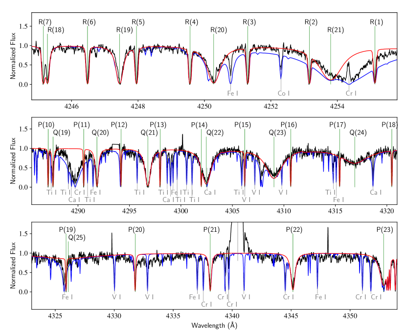
Figure 20: The same as in Fig. 15, but with atomic lines indicates: Comparison with the observed spectrum of AlH of Proxima Cen by Pavlenko et al. (2022) shown by black line for the (0-0) band spectral range. Here and onward, we have adhered to the procedure of computation and identification of spectral features outlined by Pavlenko et al. (2022). The blue line marks the synthetic spectrum including atomic and molecular species, the red line spectrum is calculated including AlH lines only.

Table 12: Re-measured astrophysical line positions in nm and cm^-1from the Proxima Cen. spectrum observed by Pavlenko et al. (2022) for the ${A}\,^{1}\Pi-{X}\,^{1}\Sigma^{+}$ system.

Band	Branch	J	$\lambda$ nm	Unc. nm	$\nu$ cm-1	Unc. cm-1	Width Å	Unc. Å
1-0	Q	2	4072.572	0.003	24547.576	0.018	0.024	0.002
1-0	Q	4	4074.981	0.003	24533.064	0.018	0.022	0.003
1-0	Q	7	4081.455	0.003	24494.151	0.018	0.032	0.002
1-0	Q	8	4084.468	0.003	24476.083	0.018	0.041	0.002
1-0	Q	9	4087.974	0.050	24455.091	0.299	0.081	0.028
1-0	Q	10	4092.080	0.060	24430.554	0.358	0.132	0.008
1-0	Q	11	4096.721	0.030	24402.878	0.179	0.281	0.007
1-0	Q	13	4108.593	0.150	24332.366	0.888	0.766	0.037
1-0	P	4	4081.951	0.003	24491.175	0.018	0.021	0.002
1-0	P	5	4085.420	0.003	24470.379	0.018	0.021	0.002
1-0	P	6	4089.261	0.003	24447.395	0.018	0.023	0.002
1-0	P	7	4093.490	0.003	24422.139	0.018	0.021	0.002
1-0	P	8	4098.126	0.003	24394.512	0.018	0.023	0.001
1-0	P	9	4103.228	0.024	24364.180	0.143	0.035	0.002
1-0	P	10	4108.813	0.003	24331.063	0.018	0.045	0.003
1-0	P	11	4114.950	0.006	24294.777	0.035	0.113	0.007
1-0	P	12	4121.753	0.006	24254.679	0.035	0.232	0.010
1-0	P	13	4129.276	0.080	24210.491	0.469	0.355	0.019
1-0	R	0	4069.800	0.003	24564.295	0.018	0.019	0.002
1-0	R	1	4068.391	0.003	24572.802	0.018	0.021	0.002
1-0	R	3	4066.623	0.003	24583.485	0.018	0.024	0.002
1-0	R	6	4066.830	0.003	24582.234	0.018	0.022	0.002
1-0	R	7	4067.757	0.003	24576.632	0.018	0.043	0.002
1-0	R	8	4069.190	0.004	24567.978	0.024	0.072	0.004
1-0	R	9	4071.185	0.003	24555.939	0.018	0.104	0.003
1-0	R	10	4073.747	0.080	24540.496	0.482	0.246	0.008
1-0	R	11	4077.140	0.010	24520.074	0.060	0.375	0.019
1-0	R	12	4081.352	0.034	24494.769	0.204	0.504	0.045
0-0	R	3	4251.300	0.003	23515.596	0.017	0.022	0.002
0-0	R	4	4249.562	0.003	23525.214	0.017	0.028	0.002
0-0	R	5	4247.955	0.003	23534.113	0.017	0.023	0.002
0-0	R	6	4246.477	0.003	23542.304	0.017	0.028	0.002
0-0	R	9	4242.978	0.003	23561.718	0.017	0.028	0.001
0-0	R	16	4242.435	0.003	23564.734	0.017	0.025	0.002
0-0	R	17	4243.632	0.003	23558.087	0.017	0.027	0.002
0-0	R	18	4245.278	0.003	23548.953	0.017	0.045	0.002
0-0	R	19	4247.462	0.010	23536.845	0.055	0.076	0.002
0-0	R	20	4250.273	0.004	23521.278	0.022	0.172	0.004
0-0	Q	9	4264.448	0.003	23443.095	0.016	0.040	0.003
0-0	Q	10	4265.689	0.003	23436.275	0.016	0.034	0.002
0-0	Q	11	4267.102	0.003	23428.515	0.016	0.032	0.002
0-0	Q	13	4270.533	0.003	23409.692	0.016	0.031	0.001
0-0	Q	14	4272.590	0.003	23398.422	0.016	0.027	0.002
0-0	Q	17	4280.475	0.003	23355.321	0.016	0.032	0.002
0-0	Q	18	4283.797	0.003	23337.210	0.016	0.042	0.002
0-0	Q	19	4287.564	0.003	23316.706	0.016	0.061	0.003
0-0	Q	20	4291.854	0.008	23293.400	0.043	0.153	0.009
0-0	Q	21	4296.784	0.004	23266.675	0.022	0.261	0.005
0-0	Q	22	4302.466	0.006	23235.948	0.032	0.385	0.006
0-0	Q	23	4309.019	0.009	23200.612	0.048	0.752	0.018
0-0	Q	24	4316.792	0.150	23158.837	0.805	1.016	0.040
0-0	P	2	4264.069	0.003	23445.179	0.016	0.018	0.002
0-0	P	4	4269.154	0.003	23417.254	0.016	0.022	0.002
0-0	P	16	4310.653	0.003	23191.818	0.016	0.026	0.002
0-0	P	17	4315.409	0.003	23166.259	0.016	0.026	0.002
0-0	P	18	4320.477	0.003	23139.085	0.016	0.029	0.002
0-0	P	19	4325.911	0.003	23110.019	0.016	0.043	0.002
0-0	P	20	4331.781	0.003	23078.704	0.016	0.063	0.003
0-0	P	21	4338.153	0.003	23044.806	0.016	0.102	0.003
0-0	P	22	4345.156	0.005	23007.665	0.026	0.180	0.005
0-0	P	23	4352.994	0.100	22966.238	0.528	0.305	0.010

References

- Antony et al. (2006) Antony B. K., Gamache P. R., Szembek C. D., Niles D. L., Gamache R. R., 2006, Mol. Phys., 104, 2791
- Baltayan & Nedelec (1979) Baltayan P., Nedelec O., 1979, J. Chem. Phys., 70, 2399
- Barklem & Collet (2016) Barklem P. S., Collet R., 2016, A&A, 588, A96
- Barton et al. (2017) Barton E. J., Hill C., Czurylo M., Li H.-Y., Hyslop A., Yurchenko S. N., Tennyson J., 2017, J. Quant. Spectrosc. Radiat. Transf., 203, 490
- Bengtsson (1928) Bengtsson E., 1928, Z. Phys., 51, 889
- Bengtsson & Rydberg (1930) Bengtsson E., Rydberg R., 1930, Z. Phys., 59, 540
- Braam et al. (2021) Braam M., van der Tak F. F. S., Chubb K. L., Min M., 2021, A&A, 646, A17
- Brault (1987) Brault J. W., 1987, Microchim. A., 93, 215
- Bruker Optik GmbH (2005) Bruker Optik GmbH ., 2005, Bruker, OPUS: spectroscopy software for state-of-the-art measurement, processing and evaluation of IR, NIR and Raman Spectra. v.8.5.29.
- Buldyreva et al. (2024) Buldyreva J., Brady R. P., Yurchenko S. N., Tennyson J., 2024, J. Quant. Spectrosc. Radiat. Transf., 313, 108843
- Challacombe & Almy (1937) Challacombe C., Almy G., 1937, Phys. Rev., 51, 0930
- Chubb & Min (2022) Chubb K. L., Min M., 2022, A&A, 665, A2
- Chubb et al. (2020) Chubb K. L., Min M., Kawashima Y., Helling C., Waldmann I., 2020, A&A, 639, A3
- Chubb et al. (2021) Chubb K. L., et al., 2021, A&A, 646, A21
- Connor & Smith (1981) Connor J., Smith A., 1981, Mol. Phys., 43, 397
- Császár et al. (2007) Császár A. G., Czakó G., Furtenbacher T., Mátyus E., 2007, Annu. Rep. Comput. Chem., 3, 155
- Deutsch et al. (1987) Deutsch J. L., Neil W. S., Ramsay D. A., 1987, J. Mol. Spectrosc., 125, 115
- Diehl et al. (2006) Diehl R., et al., 2006, A&A, 449, 1025
- Furtenbacher & Császár (2012) Furtenbacher T., Császár A. G., 2012, J. Mol. Struct., 1009, 123
- Furtenbacher et al. (2007) Furtenbacher T., Császár A. G., Tennyson J., 2007, J. Mol. Spectrosc., 245, 115
- Gee & Wasylishen (2001) Gee M., Wasylishen R. E., 2001, J. Mol. Spectrosc., 207, 153
- Gharib-Nezhad et al. (2021) Gharib-Nezhad E., Iyer A. R., Line M. R., Freedman R. S., Marley M. S., Batalha N. E., 2021, ApJS, 254, 34
- Gordy & Cook (1984) Gordy W., Cook R. L., 1984, Microwave Molecular Spectra. John Wiley & Sons
- Goto & Saito (1995) Goto M., Saito S., 1995, ApJ, 452, L147
- Grabe & Hulthén (1939) Grabe B., Hulthén E., 1939, Z. Phys., 114, 470
- Grimm et al. (2021) Grimm S. L., et al., 2021, ApJS, 253, 30
- Hakalla et al. (2017) Hakalla R., et al., 2017, J. Quant. Spectrosc. Radiat. Transf., 189, 312
- Halfen & Ziurys (2004) Halfen D. T., Ziurys L. M., 2004, ApJ, 607, L63
- Halfen & Ziurys (2010) Halfen D. T., Ziurys L. M., 2010, ApJ, 713, 520
- Halfen & Ziurys (2014) Halfen D. T., Ziurys L. M., 2014, ApJ, 791, 65
- Halfen & Ziurys (2016) Halfen D. T., Ziurys L. M., 2016, ApJ, 833, 89
- Hartmann et al. (2008) Hartmann J.-M., Boulet C., Robert D., 2008, Collisional effects on molecular spectra. Laboratory experiments and models, consequences for applications. Elsevier, Amsterdam
- Herbig (1956) Herbig G. H., 1956, PASP, 68, 204
- Herzberg (1939) Herzberg G., 1939, Molecular Spectra and Molecular Structure, Vol. 1, Diatomic Molecules. Prentice-Hall, New York, New York
- Herzberg & Mundie (1940) Herzberg G., Mundie L. G., 1940, J. Chem. Phys., 8, 263
- Holst (1933) Holst W., 1933, Z. Phys., 86, 338
- Holst (1934) Holst W., 1934, Z. Phys., 90, 735
- Holst & Hulthén (1934) Holst W., Hulthén E., 1934, Z. Phys., 90, 712
- Ito et al. (1994) Ito F., Nakanga T., Takeo H., Jones H., 1994, J. Mol. Spectrosc., 164, 379
- Johnson (2022) Johnson R. D. I., 2022, NIST Computational Chemistry Comparison and Benchmark Database
- Kaminski et al. (2016) Kaminski T., et al., 2016, A&A, 592, A42
- Khan (1958) Khan M., 1958, Proc. Phys. Soc. Lond., 71, 65
- Khan (1962) Khan M., 1962, Proc. Phys. Soc. Lond., 79, 745
- Kleman (1953) Kleman B., 1953, Ark. Fys., 6, 407
- Lagerqvist et al. (1970) Lagerqvist A., Lundh L. E., Neuhaus H., 1970, Physica Scripta, 1, 261
- Le Roy (2017) Le Roy R. J., 2017, J. Quant. Spectrosc. Radiat. Transf., 186, 167
- Le Roy et al. (2006) Le Roy R. J., Huang Y., Jary C., 2006, J. Chem. Phys., 125, 164310
- Loukhovitski & Sharipov (2021) Loukhovitski B. I., Sharipov A. S., 2021, J. Phys. Chem. A, 125, 5117
- Lyubchyk et al. (2022) Lyubchyk Y. P., Pavlenko V Y., Lyubchyk O. K., Jones H. R. A., 2022, Kinemat. Phys. Celest., 38, 159
- Ma et al. (2013) Ma Q., Boulet C., Tipping R. H., 2013, J. Chem. Phys., 139, 034305
- Marigo et al. (2022) Marigo P., Aringer B., Girardi L., Bressan A., 2022, ApJ, 940, 129
- Mayor et al. (2003) Mayor M., et al., 2003, The Messenger, 114, 20
- Nilsson (1948) Nilsson B. E., 1948, PhD thesis, University of Stockholm, https://urn.kb.se/resolve?urn=urn:nbn:se:su:diva-74489
- Niu et al. (2016) Niu M. L., Hakalla R., Trivikram T. M., Heays A. N., de Oliveira N., Salumbides E. J., Ubachs W., 2016, Mol. Phys., 114, 2857
- Palmer & Engleman (1983) Palmer B. A., Engleman R. J., 1983
- Pavlenko et al. (2022) Pavlenko Y., Tennyson J., Yurchenko S. N., Jones H. R. A., Lyubchik Y., Suárez Mascareño A., 2022, MNRAS, 516, 5655
- Pezzella et al. (2021) Pezzella M., Yurchenko S. N., Tennyson J., 2021, Phys. Chem. Chem. Phys., 23, 16390
- Pezzella et al. (2022) Pezzella M., Yurchenko S. N., Tennyson J., 2022, MNRAS, 514, 4413
- Prajapat et al. (2017) Prajapat L., Jagoda P., Lodi L., Gorman M. N., Yurchenko S. N., Tennyson J., 2017, MNRAS, 472, 3648
- Qin et al. (2021) Qin Z., Bai T., Liu L., 2021, ApJ, 917, 87
- Ram & Bernath (1996) Ram R. S., Bernath P. F., 1996, Appl. Optics, 35, 2879
- Rathcke et al. (2023) Rathcke A. D., et al., 2023, MNRAS, 522, 582
- Ryabchikova et al. (2015) Ryabchikova T., Piskunov N., Kurucz R. L., Stempels H. C., Heiter U., Pakhomov Y., Barklem P. S., 2015, Phys. Scr., 90, 054005
- Sauval & Tatum (1984) Sauval A. J., Tatum J. B., 1984, ApJS, 56, 193
- Shanmugapriya et al. (2022) Shanmugapriya G., Karthikeyan B., Rajamanickam N., Bagare S. P., 2022, Eur. Phys. J. Plus, 137, 1005
- Sindhan et al. (2023) Sindhan R., Sriramachandran P., Shanmugavel R., Ramaswamy S., 2023, New Astr., 99, 101939
- Svehla (1962) Svehla R. A., 1962, Technical Report NASA-TR-R-132, Estimated viscosities and thermal conductivities of gases at high temperatures, https://www.osti.gov/biblio/4803072. National Aeronautics and Space Administration. Lewis Research Center, Cleveland, https://www.osti.gov/biblio/4803072
- Szajna & Zachwieja (2009) Szajna W., Zachwieja M., 2009, Eur. Phys. J. D, 55, 549
- Szajna & Zachwieja (2010) Szajna W., Zachwieja M., 2010, J. Mol. Spectrosc., 260, 130
- Szajna et al. (2011) Szajna W., Zachwieja M., Hakalla R., Kepa R., 2011, Acta Phys. Pol.A, 120, 417
- Szajna et al. (2015) Szajna W., Zachwieja M., Hakalla R., 2015, J. Mol. Spectrosc., 318, 78
- Szajna et al. (2017a) Szajna W., Hakalla R., Kolek P., Zachwieja M., 2017a, J. Quant. Spectrosc. Radiat. Transf., 187, 167
- Szajna et al. (2017b) Szajna W., Moore K., Lane I. C., 2017b, J. Quant. Spectrosc. Radiat. Transf., 196, 103
- Szajna et al. (2023) Szajna W., Kȩpa R., Para A., Piotrowska I., Ryzner S., Field R. W., Heays A. N., Hakalla R., 2023, J. Mol. Spectrosc., 391, 111735
- Tao et al. (2003) Tao C., Tan X. F., Dagdigian P. J., Alexander M. H., 2003, J. Chem. Phys., 118, 10477
- Tennyson et al. (2023) Tennyson J., Pezzella M., Zhang J., Yurchenko S. N., 2023, RASTI, 2, 231
- Tóbiás et al. (2019) Tóbiás R., Furtenbacher T., Tennyson J., Császár A. G., 2019, Phys. Chem. Chem. Phys., 21, 3473
- Urban & Jones (1992) Urban R. D., Jones H., 1992, Chem. Phys. Lett., 190, 609
- Voronina & Voronin (2019) Voronina S. S., Voronin B. A., 2019, in 25th International Symposium on Atmospheric and Ocean Optics: Atmospheric Physics. , doi:10.1117/12.2540371
- Werner et al. (2020) Werner H.-J., et al., 2020, The Journal of Chemical Physics, 152, 144107
- White et al. (1993) White J. B., Dulick M., Bernath P. F., 1993, J. Chem. Phys., 99, 8371
- Wright et al. (2022) Wright S. O. M., Waldmann I., Yurchenko S. N., 2022, MNRAS, 512, 2911
- Wright et al. (2023) Wright S. O. M., et al., 2023, AJ., 166, 41
- Yamada & Hirota (1992) Yamada C., Hirota E., 1992, Chem. Phys. Lett., 197, 461
- Yurchenko et al. (2016) Yurchenko S. N., Lodi L., Tennyson J., Stolyarov A. V., 2016, Comput. Phys. Commun., 202, 262
- Yurchenko et al. (2018a) Yurchenko S. N., Sinden F., Lodi L., Hill C., Gorman M. N., Tennyson J., 2018a, MNRAS, 473, 5324
- Yurchenko et al. (2018b) Yurchenko S. N., Williams H., Leyland P. C., Lodi L., Tennyson J., 2018b, MNRAS, 479, 1401
- Yurchenko et al. (2018c) Yurchenko S. N., Al-Refaie A. F., Tennyson J., 2018c, A&A, 614, A131
- Yurchenko et al. (2023) Yurchenko S. N., Nogué E., Azzam A. A. A., Tennyson J., 2023, MNRAS, 520, 5183
- Zeeman & Ritter (1954) Zeeman P. B., Ritter G. J., 1954, Can. J. Phys., 32, 555
- Zhang et al. (2023) Zhang J., Tennyson J., Yurchenko S. N., 2023, RASTI
- Zhu et al. (1992) Zhu Y. F., Shehadeh R., Grant E. R., 1992, J. Chem. Phys., 97, 883
- Zilinskas et al. (2023) Zilinskas M., Miguel Y., van Buchem C. P. A., Snellen I. A. G., 2023, A&A, 671, A138
- van der Tak et al. (2007) van der Tak F., Black J., Schöier F., Jansen D., van Dishoeck E., 2007, A&A, 468, 627