Causality constraints on TMD soft factors: the exponential regulator without cuts

Abstract

We show that as a result of causality-constrained coordinate space analyticity, the Drell-Yan-shape transverse-momentum dependent soft factor in the exponential regulator allows below-threshold (Euclidean) parametric representations without cuts, to all orders in perturbation theory. Moreover, it is identical to another soft factor with natural interpretation as a space-like form factor, and this relation continues to hold for a larger class of TMD soft factors that interpolate between three different rapidity regulators: the off-light-cone regulator, the finite light-front length regulator, and the exponential regulator.

1 Introduction

It is known that in many UV-complete local QFTs, including QCD, the Euclidean short distance limit $-z^{2}\rightarrow 0$ or high-virtuality limit $-Q^{2}\rightarrow\infty$ for correlation functions has controlled asymptotic expansion through Lagrangian perturbation theory to the UV conformal field theories (CFTs). The corresponding Feynman integrals for Euclidean quantities are also very nice: the parametric representations $e^{-Q^{2}\rho\frac{U}{V}(x)}$ have non-oscillating positive rational functions $\frac{U}{V}(x)$ in the exponential and always decay in the large $\rho$ limit, allowing establishment of analyticity as well rigorous mathematical proofs. On the other hand, for non-Euclidean above-threshold Lorentzian quantities, the perturbation theory is generically much more singular. Not only the parameter space as well as momentum space representations become oscillating, intermediate states for amplitudes or conjugating amplitudes can even be pinched to be on-shell (namely, picking up the $\delta(E-E_{k})$ contribution from $\frac{1}{E-E_{k}\pm i0}=P\frac{1}{E-E_{k}}\mp i\pi\delta(E-E_{k})$) in a dangerous way that not only destroying analyticity, but also making the high-energy limit much less under control. Fortunately, it is known that in a few cases such dangerous contributions either cancel among themselves or are absent Collins (2013); Diehl et al. (2016), leading to factorizable form of high-energy limits Collins (2013) with universal hard kernels controlled by the same perturbation theory to the UV CFT as that for the Euclidean $z^{2}\rightarrow 0$ limit. It is therefore natural to think that if such factorizable high-energy limits, at least for the individual pieces appearing in the factorization theorems, can be approached from the below-threshold side where problems with on-shell intermediate states are absent from the beginning. Clearly, such below-threshold formulation is crucial for the Euclidean lattice approach to parton distribution functions Ji (2013, 2014); Ji et al. (2021).

The simplest limit or quantity that can be approached from the below-threshold side is the Bjorken limit, for which the Euclidean formulation suitable for lattice implementation is provided firstly in Ji (2013, 2014). The fact that PDFs or GPDs themselves are just generating functions of form factors or matrix elements of twist-two operators that allow below-threshold parametric representations (for stable external states) in perturbation theory is a primary reason why such lattice formulation ever exists. On the other hand, for transverse-momentum dependent (TMD) quantities, there are additional subtleties caused by rapidity-divergences and the corresponding rapidity regulators that might destroy the naive-looking below-threshold property. For example, the naive shape of the TMD soft factor for the Drell-Yan (DY) process is almost below-threshold in the sense that it involves only light-like and space-like mutual separations. On the other hand, the rapidity regulator may render this property less transparent. In the original formulation in Refs. Collins and Metz (2004); Collins (2013), the rapidity regulator is implemented by deforming the light-like Wilson-lines into space-like directions. As a result, in this off-light-cone regulator, the TMD soft factor is apparently below-threshold, time-ordering insensitive Collins (2013); Vladimirov (2016, 2018) and achieves universality across three standard processes $e^{+}e^{-}$, DY and semi-inclusive DIS (SIDIS). Furthermore, it has been shown in Ref. Ji et al. (2020a, 2021); Liu (2022) that the DY shape TMD soft factor in this regulator can actually be interpreted as a space-like form factor for infinitely heavy quark anti-quark pairs and allows Euclidean formulation. This serves as the foundation for the application to TMDPDFs Ji et al. (2020b) as well as light-front (LF) wave functions (LFWFs) Ji and Liu (2022). To further consolidate this result, it is important to establish such relations in other rapidity regulators, which was achieved in Ref. Liu (2022) for the $\delta$ regulator Echevarria et al. (2016a, b).

It is the purpose of this paper to show that such relations exist in the exponential regulator Li et al. (2020); Moult and Zhu (2018) as well. We demonstrate in Sec. 3 using causality-constrained coordinate-space analyticity properties reviewed in Sec. 2 for gluonic correlation functions in perturbation theory in linear covariant gauges that the DY-shape TMD soft factor in the exponential regulator allows below-threshold parametric representations and can be calculated without cuts. As a result, we show in Sec. 3 that it equals another soft factor with a natural interpretation as a space-like form factor of heavy quark anti-quark pairs, extending the previously known relations Ji et al. (2020a, 2021); Liu (2022) to the exponential regulator. This relationship is further extended to a larger class of TMD soft factors that interpolate between three regulators: the off-light-cone regulator, the exponential regulator, and the “finite light-front length” regulator Vladimirov (2018, 2020). By taking limits in different orders, one obtains the corresponding relations in all three regulators. At the end of the paper in Sec. 4, we provide a short proof that shows the equality between DY-shape and SIDIS-shape TMD soft factors in the exponential regulator, both represented initially as amplitude squares.

2 Coordinate space analyticity in local QFT

Since the TMD soft factors are naturally formulated in coordinate space, namely, they are vacuum expectation values of Wilson loops, a natural tool to investigate their properties and establish relationships is the coordinate space analyticity of local QFT. In this section we provide a brief introduction to coordinate space analyticity of Wightman functions. For more detail, see Refs. Streater and Wightman (1989); Jost (1965).

In fact, the discovery of coordinate space analyticity traces back to the 1950s. It is known Streater and Wightman (1989); Jost (1965) that given the standard Wightman axioms of locality, causality and spectral condition (positivity is not required to establish analyticity) for local QFTs, the Wightman functions of a local QFT allow analytical continuation into the “permuted extended tube” region as single-valued analytic Wightman functions instead of distributions, and the original real-time Wightman functions can all be obtained as boundary values of the analytic Wightman functions. Moreover, the analytic Wightman functions are covariant under proper complex Lorentz transforms and are symmetric or anti-symmetric under permutations. The “extended tube” can be obtained by applying complex Lorentz transforms on the “tube” region of the form ($P$ denotes a permutation of $(1,2,..,n)$)

$$\mathfrak{S}^{P}_{n}=\bigg{\{}(z_{P_{n}},z_{P_{n-1}},....z_{P_{1}});-{\rm Im}(z_{P_{k}}-z_{P_{k-1}})\in V_{+},2\leq k\leq n\bigg{\}}\ ,$$ (1)

with imaginary parts of the consecutive differences lying in the (negative) forward light-cone. The analyticity of the Wightman function

$$W(z_{P_{n}},z_{P_{n-1}},...z_{P_{1}})\equiv\langle\Omega|\phi(z_{P_{n}})....\phi(z_{P_{1}})|\Omega\rangle\ ,$$ (2)

for a local quantum field in the tube region can be established using the fact that the spectral functions are supported within the forward light-cone. One then analytically continues by applying proper complex Lorentz transforms on tube region and using the local commutativity for totally space-like separations and the “edge of the wedge” theorem to connect analytic continuations starting from $n!$ different permutations. The “extended tube” includes real points (“Jost point”) as well, and the Wightman functions are always analytic at totally space-like real separations. The real-time Wightman functions can always be obtained as boundary value of analytic Wightman functions

$$W(t_{n},...t_{1})=\lim_{\eta\rightarrow 0^{+}}W(t_{n}-i(n-1)\eta,t_{n-1}-i(n-2)\eta.....,t_{1})\ ,$$ (3)

where spatial components are omitted for simplicity. The above implies that for any time-like separation $x_{ij}^{2}=(x_{i}-x_{j})^{2}>0$ where analytic Wightman functions can develop branch cuts, the time-ordering case where $t_{i}>t_{j}$ for $i>j$ is approached above the branch cut for $-x_{ij}^{2}$, namely, $-x_{ij}^{2}=-x_{ij}^{2}+i0$, while the anti-time-ordering case is approached with $-x_{ij}^{2}-i0$. In this way, the permutation symmetry for the analytic Wightman function is broken for time-like boundary separations.

Within the analyticity region for analytic Wightman functions, one needs to mention the imaginary-time or “Euclidean” points

$${\cal E}_{n}=\bigg{\{}(z_{n},z_{n-1},....z_{1});z_{k}^{0}\equiv-ix^{4}_{k},x^{4}_{k}\in{\cal R},1\leq k\leq n;z_{i}\neq z_{j},\forall i\neq j\bigg{\}}\ .$$ (4)

Restriction of analytic Wightman functions in the above Euclidean points are called “Schwinger functions” or “Euclidean-time Green functions”. The Euclidean-time Green functions are invariant under rotations and are symmetric or anti-symmetric under permutations. Moreover, starting from a complete set of Schwinger functions satisfying the Osterwalder-Schrader axioms Osterwalder and Schrader (1973, 1975) requiring rotational invariance, moderate growth speed and the reflection positivity, one can analytically continue back from Euclidean signature to Lorentzian signature to obtain a complete set of real-time Wightman functions satisfying the Wightman axioms. This fact forms the foundation for the standard Euclidean approach to QFTs, which identifies Schwinger functions of a local QFT as scaling limits of correlation functions in near-critical cutoff models. A simple demonstration-of-principle example of such relation is actually the 2D Ising model, for which the massive scaling functions at $h=0$ have nice analytical representations Wu et al. (1976); McCoy et al. (1977), and there are many examples that were established using expansion methods (for example, the asymptotically-free 2D massive Gross-Neveu in Feldman et al. (1985, 1986)). Due to the criticality of the cutoff theories, QFTs constructed in the above manner usually have scale-invariant short-distance limits characterized by conformal field theories. Although CFTs are more singular than massive QFTs, since they represent short distance singularities for massive QFTs, they actually inherited the full analyticity structure of Wightman functions for the massive QFTs as well Luscher and Mack (1975); Hartman et al. (2016), which forms the foundation for recent applications in Caron-Huot (2017); Caron-Huot and Sandor (2021).

Since the UV limit of a local QFT usually has asymptotic descriptions in terms of local, covariant perturbations to the UV CFT, it is natural to consider analyticity structure in such perturbation theory. In this work, we only consider the case where the UV CFT is free (such as free gluons in the Feynman gauge), and the dimensional regularization (DR) can be consistently implemented to all orders. In this case, the resulting coordinate space Wightman functions, up to pre-factors which are polynomials in $x_{ij}^{\mu}$ taking care of the tensor structure of the Wightman functions and are apparently analytic and covariant, have below-threshold parametric representations for totally space-like and imaginary-time separations ${\cal E}_{n}$ in terms of the “scalar-integrals” of the following form

$$I(x_{E,ij}^{2}\equiv-x_{ij}^{2})=\int_{0}^{\infty}D\alpha U(\alpha,\epsilon)e^{-\sum_{i<j}P_{ij}(\alpha)x_{E,ij}^{2}}\ ,$$ (5)

where the rational functions $P_{ij}(\alpha)$ are $\epsilon$ independent and positive. An inductive proof for Eq. (5) including positivity for $P_{ij}(\alpha)$ has been given in Appendix.C of Ji et al. (2023). More precisely, for a connected Feynman diagram $G$ without tadpoles (lines that start and end at the same point) and without direct connections between external vertices (since they factorize) one has

$$P_{ee^{\prime}}(\alpha)=\frac{\sum_{{\cal L}\in{\cal L}(e,e^{\prime})}\bigg{(}\prod_{\alpha\in{\cal L}}\alpha^{-1}\bigg{)}\sum_{{\cal T}\in{\cal T}_{1}\left(G/(E\bigcup{\cal L})\right)}\prod_{\alpha\in{\cal T}}\alpha^{-1}}{4\sum_{{\cal T}\in{\cal T}_{1}\left(G/E\right)}\prod_{\alpha\in{\cal T}}\alpha^{-1}}\ ,$$ (6)

where $E$ is the set of external vertices, ${\cal L}(e,e^{\prime})$ is the set of connected paths passing through internal vertices connecting $e$ and $e^{\prime}$ , $G/E$ is the diagram obtained by contracting all the points in $E$ to a single point and then deleting tadpoles, and ${\cal T}_{1}(G)$ is the set of spanning trees for the diagram $G$. Equation (6) can be proven using the “all minors matrix tree theorem” Bogner and Weinzierl (2010), see Appendix. A for more details and a concrete example. Clearly, the above form of parameter space integral is similar to the “below-threshold” momentum space integrals characterized by non-alternating negative functions in the exponential. Therefore, similar to the momentum-space cases, the above scalar integrals actually define single-valued analytic functions in $\eta_{ij}=-x_{ij}^{2}$ not only for totally space-like and Euclidean separations, but also in the following permutation-symmetric “below-threshold region”

$${\cal E}_{n}\subset{\cal E}_{n}^{\prime}=\bigg{\{}(z_{n},z_{n-1},...z_{1});\ {\rm Re}(z_{ij}^{2})<0\ ,\forall i<j\bigg{\}}\ ,$$ (7)

due to the fact that in this region, the parametric integral Eq. (5) is uniformly bounded by the real part in the exponential. Notice an arbitrary point in ${\cal E}_{n}^{\prime}$ always connects to the Euclidean region ${\cal E}_{n}$ through a connected path in ${\cal E}_{n}^{\prime}$. Furthermore, the common region $\mathfrak{S}_{n}^{P}\bigcap{\cal E}_{n}^{\prime}$ for any permutation $P$ is path-connected (see Appendix. B for a proof) and contains $\mathfrak{S}_{n}^{P}\bigcap{\cal E}_{n}$ as a “real environment”. As a result, after combining scalar integrals with pre-factors, the Euclidean parametric representations uniquely continue the perturbative analytic Wightman functions into the region ${\cal E}_{n}^{\prime}$ . They are symmetric or anti-symmetric under permutations after summing over all the diagrams at any given order, and are apparently covariant under complex Lorentz transformations (since both the tensorial pre-factors and the invariant length-squares $\eta_{ij}$ are apparently covariant.)

One should also mention that these analytic Wightman functions, when continued further to time-like separation for any real $x^{2}_{ij}>0$, may develop branch cuts. In such cases, the time-ordering is approached above the branch cut with $-x_{ij}^{2}+i0$ prescription, while the anti-time-ordering case is approach below the branch cut with $-x^{2}_{ij}-i0$ prescription. It is easy to check that in case where all the separations are time-ordered, the analytic continuation of the below-threshold or Euclidean parametric integral in Eq. (5) for any real-time separations can be implemented at the level of parametric representations and are simply given by the standard Lorentzian signature parametric integrals with $i$ in the exponential. In fact, such relation, when flipped the order, is nothing but the standard coordinate space version of the “Wick-rotation”. On the other hand, if both time-orderings for time-like separations are present, then the analytical continuation at the level of parametric representation can be non-trivial. One way to perform the analytic continuation in such situation is to convert to the “Mellin represantation” using

$$e^{-P_{ij}(\alpha)x_{E,ij}^{2}}=\int_{c-i\infty}^{c+i\infty}\frac{dt_{ij}}{2\pi i}(P_{ij}(\alpha))^{-t_{ij}}\Gamma(t_{ij})(x_{E,ij}^{2})^{-t_{ij}}\ ,$$ (8)

and analytically continues with $x_{E,ij}^{2}\rightarrow-x_{ij}^{2}+i(i-j)(t_{i}-t_{j})\eta$ under Eq. (8) after integrating over the $\alpha$ parameters (which can introduce additional suppression functions). It is not clear that this procedure always work, but fortunately in this paper we can completely avoid problems with analytical continuation for time-like separations, as all the separations involved in this paper (except for the discussions at the end of the paper in Sec. 4 which is based on old-fashioned perturbation theory instead of coordinate analyticity) are either within (or approached within) $\mathfrak{S}^{P}_{n}\bigcap{\cal E}_{n}^{\prime}$ or inside a single time-ordering.

In the following sections, we will investigate the DY-shape TMD soft factor in the exponential rapidity regulator, from the perspective of coordinate space analyticity. We will use the fact that in linear covariant gauges, spectral condition as well as local commutativity for gluon fields hold to all orders , and perturbative Wightman functions for gluon fields are Lorentz-covariant and allow below-threshold parametric representations of the form Eq. (5) for totally space-like and imaginary-time separations, implying analyticity as well as permutation symmetry and covariance under complex Lorentz transformation, in the regions $\mathfrak{S}_{n}^{P}\bigcap{\cal E}_{n}^{\prime}$. We will show that the DY-shape TMD soft factor in the exponential regulator, although initially calculated through cuts mimicking “amplitude squares” for total cross-section, has below-threshold parametric representations similar to Eq. (7) without cuts. Moreover, we will show that it actually equals another soft factor, which can be interpreted as a space-like form factor, and generalize this relationship by simultaneously including the off-light-cone regulator and the finite LF length regulator.

3 The exponential regulator without cuts

As proposed in 2016 Li et al. (2020), the DY TMD soft factor in the exponential regulator is defined as a specific Wilson-loop average. To simply the notation, one introduces the light-like Wilson-lines as

$$W_{n}(x)={\cal P}\exp\bigg{[}-ig\int_{-\infty}^{0}d\lambda n\cdot A(x+\lambda n)\bigg{]}\ ,$$ (9)

$$W_{\bar{n}}(x)={\cal P}\exp\bigg{[}-ig\int_{-\infty}^{0}d\lambda\bar{n}\cdot A(x+\lambda\bar{n})\bigg{]}\ ,$$ (10)

where the light-like directions read

$$n=\frac{1}{\sqrt{2}}(1,1,\vec{0}_{\perp})\ ,$$ (11)

$$\bar{n}=\frac{1}{\sqrt{2}}(1,-1,\vec{0}_{\perp})\ .$$ (12)

Without otherwise mentioning, the gluon fields $A(x)=A^{\mu,a}(x)t^{a}$ are in fundamental representations of $SU(N)$ groups and all the results can be generalized to adjoint representations as well. We will use the following notations for conjugating Wilson-lines

$$W_{n}^{\dagger}(x)={\cal P}\exp\bigg{[}-ig\int_{0}^{-\infty}d\lambda n\cdot A(x+\lambda n)\bigg{]}\ ,$$ (13)

$$W_{n}^{\dagger}(-i\nu e_{t},x)={\cal P}\exp\bigg{[}-ig\int_{0}^{-\infty}d\lambda\cdot A(x-i\nu e_{t}+\lambda n)\bigg{]}\ ,$$ (14)

where $x$ is a real vector, $\nu>0$ is a real number and $e_{t}=(1,0,0,0)$ is the unit vector in the time direction. Expressions for $W_{\bar{n}}^{\dagger}$s are similar and omitted for simplicity. In terms of these Wilson lines, the DY shape TMD soft factor in the exponential regulator reads for $\nu>0$

$$S(b_{\perp},\nu,\epsilon)=\frac{1}{N_{c}}{\rm Tr}\langle\Omega|\bar{T}W_{n}^{\dagger}(-i\nu e_{t},\vec{b}_{\perp})W_{\bar{n}}(-i\nu e_{t},\vec{b}_{\perp})TW_{\bar{n}}^{\dagger}(0)W_{n}(0)|\Omega\rangle\ ,$$ (15)

where $T$, $\bar{T}$ are the time-ordering and anti-time-ordering operators acting on $A^{\mu,a}$s. Throughout this work, we only consider perturbative soft factors in the standard dimensional regularization $D=4-2\epsilon$ for UV and IR divergences. $\epsilon$ will always be kept non-vanishing ($\epsilon\neq 0$) in the discussion unless otherwise specified, while $\mu,g$ will be omitted in all the argument lists for notation simplicity. Clearly, the above soft factor can be calculated through amplitude squares

$$S(b_{\perp},\nu,\epsilon)=\sum_{m}\int d\Pi_{m}|\langle m|TW_{\bar{n}}^{\dagger}W_{n}|\Omega\rangle|^{2}e^{i\vec{k}_{m}\cdot\vec{b}_{\perp}-\nu E_{m}}\ .$$ (16)

Here, the amplitude $\langle m|TW_{\bar{n}}^{\dagger}W_{n}|\Omega\rangle$ represents the soft approximation to the amplitude for the DY pair production process $q_{n}+\bar{q}_{\bar{n}}\rightarrow\gamma+m$ where $\gamma$ is the time-like virtual photon and $m$ is the partonic final state. The factor $e^{-\nu E_{m}}=e^{-\frac{\nu}{\sqrt{2}}\sum_{i}\left(\frac{k_{\perp,i}^{2}}{2k^{+}_{i}}+k_{i}^{+}\right)}$ regulates all the rapidity divergences caused by real emissions with $k^{+}\rightarrow 0$ or $k^{+}\rightarrow\infty$. On the other hand, the soft factor in Eq. (15) is formulated naturally in coordinate space and can be expressed in terms of line-integrals of coordinate space gluonic Wightman functions in perturbative calculations as adopted in Korchemskaya and Korchemsky (1992); Korchemsky and Marchesini (1993). This suggests us to investigate the underlying Wightman functions of gluons fields to search for representations without cuts.

3.1 Below threshold representation for DY TMD soft factor in the exponential regulator

To proceed, it is convenient to introduce the following parameterization to label an arbitrary set of non-coincidental points picked up from the Wilson lines in Eq. (15). For all the points picked up under the $T$, we chose the following representation

$$\lambda^{R}_{i}n^{R}_{i}\ ,\ -\infty<\lambda^{R}_{1}<\lambda^{R}_{i}<....<\lambda^{R}_{m_{R}}<0\ .$$ (17)

Here $n^{R}_{i}$ can be $n$ or $\bar{n}$. Clearly, the $m_{R}$ points chosen in the above manner are naturally time-ordered. Similarly, for all the points picked up under the $\bar{T}$, we chose to label them as

$$\lambda^{L}_{i}n^{L}_{i}-i\nu e_{t}-\vec{b_{\perp}}\ ,\ 0>\lambda^{L}_{1}>\lambda^{L}_{2}>....>\lambda^{L}_{m_{L}}>-\infty\ .$$ (18)

Clearly, the $m_{L}$ points above are naturally anti-time-ordered. Then, the gluonic Wightman functions involved here read (color indices play no role here and are omitted for simplicity)

$$W^{\mu^{L}_{m_{L}}...\mu^{L}_{1}\mu^{R}_{m_{R}}...\mu^{R}_{1}}(\lambda^{L}_{m_{L}}n^{L}_{m_{L}}-i\nu e_{t}-\vec{b}_{\perp},...,\lambda^{L}_{1}n^{L}_{1}-i\nu e_{t}-\vec{b}_{\perp},\lambda^{R}_{m_{R}}n^{R}_{m_{R}},....,\lambda^{R}_{1}n^{R}_{1})\ ,$$ (19)

which contract with the direction vectors $n^{L}_{m_{L}}$ to $n_{1}^{R}$. They are clearly boundary values ($\eta\rightarrow 0^{+}$ limit) of the analytic Wightman functions in the forward tube region $\mathfrak{S}_{m_{R}+m_{L}}$ in Eq. (1) through the prescription Eq. (3). To see if they allow below-threshold parametric presentations, one needs to consider the invariant length squares $-x_{ij}^{2}$ for them. The results can be enumerated as below (for items 1 to 3, adding the $-i\eta e_{t}$s with $\eta>0$ will only decrease the real parts for invariant length squares, hence only the $\eta\rightarrow 0^{+}$ limits are shown).

1. Two points under the $T$ on different Wilson lines: $(n\lambda^{R}_{i}-\bar{n}\lambda^{R}_{j})^{2}=-2\lambda^{R}_{i}\lambda^{R}_{j}<0$. The separation is space-like. The same is true for two points under the $\bar{T}$ on different Wilson lines.

2. One point under $T$, another under $\bar{T}$, on the same Wilson line direction: $(\lambda^{L}_{i}n-i\nu e_{t}-\vec{b}_{\perp}-\lambda^{R}_{j}n)^{2}=-\nu^{2}-b_{\perp}^{2}-\sqrt{2}i\nu(\lambda^{L}_{i}-\lambda^{R}_{j})$. The real part of the invariant length square is negative and bounded from above by $-b_{\perp}^{2}-\nu^{2}$.

3. One point under $T$, another under $\bar{T}$, chosen from different Wilson line directions: $(\lambda^{L}_{i}n-i\nu e_{t}-\vec{b}_{\perp}-\lambda^{R}_{j}\bar{n})^{2}=-\nu^{2}-b_{\perp}^{2}-2\lambda_{i}^{L}\lambda^{R}_{j}-\sqrt{2}i\nu(\lambda_{i}^{L}-\lambda^{R}_{j})$. The real part of the invariant length square is negative and bounded from above by $-b_{\perp}^{2}-\nu^{2}$.

4. Two points under the same $T$ or $\bar{T}$ but on the same Wilson-line. This case looks most tricky, as the separation is light-like. On the other hand, the $i\eta$ prescription in Eq. (3) resolves the problem: for $\lambda^{R}_{i}>\lambda^{R}_{j}$, the light-cone limit should be taken as the $\eta\rightarrow 0^{+}$ limit for $(\lambda^{R}_{i}n-\lambda^{R}_{j}n-i\eta(i-j)e_{t})^{2}=-(i-j)^{2}\eta^{2}-\sqrt{2}i\eta(i-j)(\lambda^{R}_{i}-\lambda^{R}_{j})$. The real part of the invariant length square is again negative for any $\eta>0$ and the light-cone limit is approached from the below-threshold region instead of time-like region. The same applies to two points in the same Wilson line under the $\bar{T}$ as well.

To summarize, for any finite $\eta>0$, the underlining separations are in $\mathfrak{S}_{m_{R}+m_{L}}\bigcap{\cal E}^{\prime}_{m_{R}+m_{L}}$. In the $\eta\rightarrow 0^{+}$ limit, the only invariant length squares for which real parts vanish correspond to null-separations on the same Wilson-lines. This already implies the existence of below-threshold parameter space representations for the Wightman functions with $\eta$ in the invariant lengths. Here we show that the $\eta\rightarrow 0^{+}$ limit for them can be further taken at the beginning.

First, the diagrams that are most sensitive to null-separations, the connected components of gluonic Wightman functions which connect only points belonging to the same Wilson-line (Wislon-line self-interactions) in the $\eta\rightarrow 0^{+}$ limit are scaleless and vanish in DR. As a result, we only need to consider diagrams in the absence of self-connecting components. For these diagrams, there are always non-vanishing invariant length squares with negative real parts at $\eta=0$ (the whole exponential never becomes light-like), and the invariant length squares

$$-(i-j)^{2}\eta^{2}-\sqrt{2}i\eta(i-j)(\lambda^{R}_{i}-\lambda^{R}_{j})\ ,$$ (20)

that vanish as $\eta\rightarrow 0^{+}$ actually serve as regulator for possible light-cone singularities within $T$ or $\bar{T}$ (namely, the “virtual loops”). On the other hand, these light-cone singularities are regulated by the dimensional regularization already, implying that the limit $\eta\rightarrow 0^{+}$ can be taken within the parametric representations of the form Eq. (5) without causing un-regularized divergences. This is also how the calculations using cuts are being performed (taking the light-cone limit for all the eikonal-propagators in the virtual loops at the beginning). The resulting parametric representations are still below-threshold with negative real parts in the exponential.

As a result, we have shown that for any $m_{L}+m_{R}$ points picked up from the Wilson loop, the corresponding gluon Wightman functions in Eq. (19) in the $\eta\rightarrow 0^{+}$ limit allow below-threshold parametric representations in terms of invariant length squares of the following types

$$x_{A,ij}^{2}=-2\lambda^{R}_{i}\lambda^{R}_{j}\ ,$$ (21)

$$x_{B,ij}^{2}=-\nu^{2}-b_{\perp}^{2}-\sqrt{2}i\nu(\lambda^{L}_{i}-\lambda^{R}_{j})\ ,$$ (22)

$$x_{C,ij}^{2}=-\nu^{2}-b_{\perp}^{2}-2\lambda_{i}^{L}\lambda^{R}_{j}-\sqrt{2}i\nu(\lambda_{i}^{L}-\lambda^{R}_{j})\ .$$ (23)

Notice that all the imaginary parts are always accompanied by strictly negative real parts bounded from above by $-b^{2}_{\perp}-\nu^{2}<0$. Moreover, the corresponding Wightman functions are symmetric under permutations and insensitive to how one orders these points. Given the Wightman functions, one simply integrates all the $\lambda$s to obtain the TMD soft factor. No divergences will be generated again, as far as $\epsilon$ and $\nu$ are both non-vanishing. In fact, for $\nu=0$, the above are just the invariant length squares for the naive DY-shape TMD soft factor. For both the $\delta$-regulator or the “finite-length” regulator Vladimirov (2018, 2020) where the Wilson lines are finite in the LF directions, namely, $[-L^{+}n,0]$ and $[-L^{-}n,0]$, one can use the above invariant lengths directly in the parametric representations to calculate the TMD soft factors in these regulators, which is also equivalent to calculating through Feynman integrals without cuts under a single time-ordering prescription Vladimirov (2016, 2018). This “time-ordering-insensitivity” for DY-shape TMD soft factor due to the fact that the underlining separations are only space-like and light-like is also crucial in order to establish the “soft-rapidity” correspondence Vladimirov (2017, 2018).

Since the only obstacle to argue for the “time-ordering-insensitivity” in the two other regulators above, as well as the $\eta\rightarrow 0$ limit for the below-threshold representation in the exponential regulator are the null separations among the same Wilson-lines, one can also get rid of them in the following way. Instead of starting from the light-like vectors, one can deform them into space-like directions as Collins and Metz (2004); Collins (2013)

$$n\rightarrow n_{Y}=n-e^{-Y}\bar{n}\ ,$$ (24)

$$\bar{n}\rightarrow\bar{n}_{Y}=\bar{n}-e^{-Y}n\ .$$ (25)

Throughout this paper we only consider $Y>0$. For arbitrary $m_{R}+m_{L}$ points chosen from the above Wilson-loop, clearly all the separations, including those self-connections, are below-threshold and the corresponding Wightman functions allow below-threshold parametric representations with $Y$-dependent invariant lengths. On the other hand, in this case, the $Y\rightarrow\infty$ limit is UV in nature and regulated by DR for any Wigthman function with finite $\lambda$s or the corresponding TMD soft factor in the simultaneous presence of finite length regulator $L^{+}$ and $L^{-}$. One then sets the invariant lengths for all the null separations to zero, or the $Y\rightarrow\infty$ limit in the parametric representations and obtains the corresponding parametric representations with the limiting invariant length squares in Eq. (21),(22), (23), in the presence of both $L^{\pm}$, $\epsilon$ and $\nu$. One then takes the $L^{\pm}\rightarrow\infty$ limit, in the presence of the two remaining regulators $\nu$ and $\epsilon$. This finally leads to the TMD soft factor in the exponential regulator expressed in terms of parametric representations with below-threshold invariant lengths Eq. (21),(22), (23), up to possible “boundary terms”. These boundary terms, if exist, can be further cancelled in a gauge-invariant way by rectangular Wilson-loops similar to the wave function renormalization factors for heavy-quark pairs introduced in Collins (2008); Ji et al. (2019, 2020b, 2020a). We will discuss this point in the paragraph of Eq. (54), after introducing the soft factor $S(L^{+},L^{-},b_{\perp},\nu,Y,\epsilon)$ in Eq. (3.2).

3.2 Equality of soft factors

To summarize, we have shown that the DY-shape TMD soft factor in the exponential regulator has below threshold representations in terms of the natural invariant length squares Eq. (21),(22), (23). The underlining gluonic Wightman functions restricted to these invariant length squares are clearly symmetric under permutation and covariant under complex Lorentz transforms. As we demonstrate in this subsection, the above implies a crucial relationship between soft factors that interprets the DY-shape soft factor as a space-like form factor instead of amplitude square.

To be more precise, let’s introduce the “future-pointing” light-like Wilson-line

$$W_{\bar{n}+}(x)={\cal P}\exp\bigg{[}-ig\int_{0}^{\infty}d\lambda\bar{n}\cdot A(x+\lambda\bar{n})\bigg{]}\ .$$ (26)

In terms of the above, we define the “form-factor shape” TMD soft factor as

$$S_{t}(b_{\perp},\nu,\epsilon)=\frac{1}{N_{c}}{\rm Tr}\langle\Omega|TW^{\dagger}_{n}(-\nu e_{z}+\vec{b}_{\perp})W^{\dagger}_{\bar{n}+}(-\nu e_{z}+\vec{b}_{\perp})W_{\bar{n}+}(0)W_{n}(0)|\Omega\rangle\ ,$$ (27)

where $e_{z}=(0,1,0_{\perp})$ is the unit vector in $z$ direction. Notice that the soft factor is under a single time-ordering. Due to this. $S_{t}$ can be interpreted as a transition amplitude for the process where a pair of quark anti-quark, separated at $\vec{b}_{\perp}-\nu e_{z}$, traveling in the light-like direction from $t=-\infty$ to $t=0$, and then changes the velocity direction from $e_{z}$ to $-e_{z}$ and propagates to $t=\infty$. As such, it can be regarded as a space-like form factor. Below we show that it actually equals the DY-shape TMD soft factor in Eq. (15).

The first argument we provide is directly based on parametric representation. In fact, it is convenient to consider the invariant length-squares for two arbitrary points selected from the Wilson-loop for $S_{t}$. They can still be enumerated as follows

1. One from $W_{n}(0)$ with $\lambda_{i}^{R}n$ where $\lambda^{R}_{i}<0$, another from $W_{\bar{n}+}(0)$ with $-\lambda^{R}_{j}\bar{n}$ where $\lambda^{R}_{j}<0$: $(\lambda^{R}_{i}\bar{n}+\lambda^{R}_{j}n)^{2}=2\lambda^{R}_{i}\lambda^{R}_{j}$ . Similar for the case between $W_{n}^{\dagger}$ and $W^{\dagger}_{\bar{n}+}$.

2. One from $W_{n}(0)$ and another from $W^{\dagger}_{n}(-\nu e_{z}+\vec{b}_{\perp})$: $(\lambda^{L}_{i}n-e_{z}\nu-\vec{b}_{\perp}-\lambda^{R}_{j}n)^{2}=-\nu^{2}-b_{\perp}^{2}+\sqrt{2}\nu(\lambda^{L}_{i}-\lambda^{R}_{j})$.

3. One from $W_{n}(0)$ and another from $W^{\dagger}_{\bar{n}^{+}}(-\nu e_{z}+\vec{b}_{\perp})$: $(-\lambda_{i}^{L}\bar{n}-\nu e_{z}+\vec{b}_{\perp}-\lambda^{R}_{j}n)^{2}=2\lambda^{L}_{i}\lambda^{R}_{j}+\sqrt{2}\nu(\lambda^{L}_{i}-\lambda^{R}_{j})-b_{\perp}^{2}-\nu^{2}$.

4. One from $W_{\bar{n}+}(0)$ and another from $W_{n}^{\dagger}(-\nu e_{z}+\vec{b}_{\perp})$: $(\lambda_{i}^{L}n-\nu e_{z}+\vec{b}_{\perp}+\lambda^{R}_{j}\bar{n})^{2}=2\lambda^{L}_{i}\lambda^{R}_{j}+\sqrt{2}\nu(\lambda^{L}_{i}-\lambda^{R}_{j})-b_{\perp}^{2}-\nu^{2}$  .

Again, null-separations are set to zero from the beginning for the same reason. From the above, one can make the following important observation: under the “Wick-rotation” $\lambda^{R}_{i}\rightarrow-i\lambda^{R}_{i}$ and $\lambda^{L}_{j}\rightarrow-i\lambda^{L}_{j}$, the above are in one-to-one correspondence with the corresponding invariant length squares Eq. (21),(22), (23) for the DY-shape soft factor. As a result, when combined with the Wick-rotation $\alpha\rightarrow-i\alpha$ for the corresponding $\alpha$ parameters, Lorentzian parametric representations for $S_{t}$ becomes exactly the below-threshold parametric representations for $S$. To show that the simultaneous Wick-rotation can be performed naturally in the $\int d\lambda d\alpha$ integrals without introducing exponential growth in the parametric space representation, it is sufficient to consider the one-loop example

$$-i\frac{2\lambda^{L}_{i}\lambda^{R}_{j}+\sqrt{2}(\lambda^{L}_{i}-\lambda^{R}_{j})\nu-b_{\perp}^{2}-\nu^{2}-i0}{4\alpha}\ .$$ (28)

Now, the Wick-rotation can be performed as follows. First, one re-scales $\lambda=\tilde{\lambda}\alpha$, then the exponential reads

$$-\frac{1}{2}i\tilde{\lambda}_{i}^{L}\tilde{\lambda}^{R}_{j}\alpha+i\frac{b_{\perp}^{2}+\nu^{2}}{4\alpha}-\frac{i\sqrt{2}(\tilde{\lambda}^{L}_{i}-\tilde{\lambda}^{R}_{j})\nu}{4}\ .$$ (29)

Now, one rotates $\alpha=-i\rho$ (without introducing exponential growth), which leads to

$$-\frac{1}{2}\tilde{\lambda}_{i}^{L}\tilde{\lambda}^{R}_{j}\rho-\frac{b_{\perp}^{2}+\nu^{2}}{4\rho}-\frac{i\sqrt{2}(\tilde{\lambda}^{L}_{i}-\tilde{\lambda}^{R}_{j})\nu}{4}\ .$$ (30)

One now re-scales back $\tilde{\lambda}=\frac{\lambda}{\rho}$, which leads to

$$-\frac{2\lambda_{i}^{L}\lambda^{R}_{j}+\nu^{2}+b_{\perp}^{2}+i\sqrt{2}(\lambda^{L}_{i}-\lambda^{R}_{j})\nu}{4\rho}\ ,$$ (31)

nothing but the below-threshold parametric space representation for the invariant lengths Eq. (23). Moreover, it is not hard to see that the gluonic Wightman functions underlining $S_{t}$, after Wick-rotating in $\lambda$s and after contracting with the direction vectors, simply differs from that for $S$ in Eq. (19) by an overall factor of the form $i^{m_{n}}(-i)^{m_{\bar{n}}}$. This factor then cancels with the factor $(-i)^{m_{n}}(i)^{m_{\bar{n}}}$ generated from $\int d\lambda$ integrals, which in turn implies that the full $\int d\lambda d\alpha$ below-threshold parametric representations for $S$ and $S_{t}$ are actually identical. In fact, the gluonic Wightman functions for $S_{t}$ after Wick-rotating in $\lambda$ simply relate to that for $S$ by a proper complex Lorentz transform

$$\Lambda(t,z)=(iz,it)\ ,$$ (32)

and the equality can be seen directly from the covariance of the gluon-Wightman functions under complex Lorentz transforms. In fact, under this transformation, one has

$$\Lambda(-i\lambda n)=\lambda n\ ,$$ (33)

$$\Lambda(-i\lambda\bar{n})=-\lambda\bar{n}\ ,$$ (34)

$$\Lambda(-\nu e_{z})=-i\nu e_{t}\ .$$ (35)

As a result, the Wilson-loop for $S_{t}$ with $\lambda\rightarrow-i\lambda$, including the integration paths, after the complex-Lorentz transform, maps exactly to that for $S$.

In fact, this relation can be generalized by including off-light-cone regulator and the finite light-front length regulator simultaneously on top of the exponential regulator. For this purpose, one introduces time-like vectors

$$v=n+e^{-Y}\bar{n}\ ,$$ (36)

$$v^{\prime}=\bar{n}+e^{-Y}n\ .$$ (37)

It is easy to show that under the complex Lorentz transform $\Lambda$, they transform into space-like vectors up to overall factors of $\pm i$

$$\Lambda v=in_{Y}\ ,$$ (38)

$$\Lambda v^{\prime}=-i\bar{n}_{Y}\ .$$ (39)

Now, lets introduce the “finite-time” versions of the Wilson-lines with $T_{1},T_{2}>0$

$$W_{v^{\prime}}(x;T_{1})={\cal P}\exp\bigg{[}-igT_{1}\int_{0}^{1}dsv^{\prime}\cdot A(x+v^{\prime}T_{1}s)]\ ,$$ (40)

$$W_{v}(x;T_{2})={\cal P}\exp\bigg{[}-igT_{2}\int_{-1}^{0}dsv\cdot A(x+vT_{2}s)]\ .$$ (41)

They can all be regarded as propagators for moving heavy-quarks in the infinitely quark mass limit. Similarly, one introduces for $L^{+},L^{-}>0$

$$W_{n_{Y}}(x;L^{+})={\cal P}\exp\bigg{[}-igL^{+}\int_{-1}^{0}dsn_{Y}\cdot A(x+n_{Y}L^{+}s)]\ ,$$ (42)

$$W_{\bar{n}_{Y}}(x;L^{-})={\cal P}\exp\bigg{[}-igL^{-}\int_{-1}^{0}ds\bar{n}_{Y}\cdot A(x+\bar{n}_{Y}L^{-}s)]\ .$$ (43)

One further introduces the corresponding conjugating Wilson-lines in a way similar to Eq. (13) and Eq. (14). In terms of them, one defines

$$S(L^{+},L^{-},b_{\perp},\nu,Y,\epsilon)=$$

$$\frac{{\rm Tr}\langle\Omega|\bar{T}W_{n_{Y}}^{\dagger}(-i\nu e_{t},\vec{b}_{\perp};L^{+})W_{\bar{n}_{Y}}(-i\nu e_{t},\vec{b}_{\perp};L^{-})TW_{\bar{n}_{Y}}^{\dagger}(0;L^{-})W_{n_{Y}}(0;L^{+})|\Omega\rangle}{{\rm Tr}\langle\Omega|\bar{T}W_{n_{Y}}^{\dagger}(-i\nu e_{t},\vec{b}_{\perp};L^{+}+L^{-})TW_{n_{Y}}(0;L^{+}+L^{-})|\Omega\rangle}\ ,$$ (44)

and

$$S_{t}(T_{1},T_{2},b_{\perp},\nu,Y,\epsilon)=$$

$$\frac{{\rm Tr}\langle\Omega|TW^{\dagger}_{v}(-\nu e_{z}+\vec{b}_{\perp};T_{2})W^{\dagger}_{v^{\prime}}(-\nu e_{z}+\vec{b}_{\perp};T_{1})W_{v^{\prime}}(0;T_{1})W_{v}(0;T_{2})|\Omega\rangle}{{\rm Tr}\langle\Omega|TW^{\dagger}_{v}(-\nu e_{z}+\vec{b}_{\perp};T_{1}+T_{2})W_{v}(0;T_{1}+T_{2})|\Omega\rangle}\ .$$ (45)

“Transverse gauge-links” along directions $\vec{b}_{\perp}-i\nu e_{t}$ or $\vec{b}_{\perp}-\nu e_{z}$ can be added at appropriate places to maintain gauge-invariance without causing additional troubles, for notation simplicity they are omitted from the equations. See discussions in the first paragraph of Sec.4 for more details regarding the “transverse gauge-links”. Furthermore, we have introduced “rectangular Wilson loops” or the $Z$ factors in the denominators playing the role of “LSZ-reduction factor” for the gauge-link pairs, in a way similar to Ji et al. (2020a). Notice that due to the overall time-ordering for $S_{t}$, one actually has $T_{1}=T_{1}(1-i0)$, $T_{2}=T_{2}(1-i0)$. $S_{t}$ can be interpreted as the real-time “transition-amplitude” for a moving heavy quark anti-quark pair and allows the analytic continuation into Euclidean time.

$$T_{1}\rightarrow-iL^{-}\ ,$$ (46)

$$T_{2}\rightarrow-iL^{+}\ .$$ (47)

Notice that an arbitrary set of non-coincidental points selected from the Wilson-loop in the numerator and denorminators for $S_{t}$ are naturally ordered in real time $t$, which becomes the Euclidean time ordering after the analytical continuation $\lambda\rightarrow-i\lambda$. The consecutive differences between them take the form

$$-i(s_{1}-s_{2})L^{-}v^{\prime}+\text{real part}\ ,\ 1>s_{1}>s_{2}>0\ ,$$ (48)

$$-i(s_{1}L^{-}v^{\prime}-s_{1}^{\prime}L^{+}v)+\text{real part}\ ,\ 1>s_{1}>0>s_{1}^{\prime}>-1\ ,$$ (49)

$$-i(s_{1}^{\prime}-s_{2}^{\prime})L^{+}v+\text{real part}\ ,\ 0>s_{1}^{\prime}>s_{2}^{\prime}>-1\ ,$$ (50)

$$-i(s_{1}^{\prime}-s_{2}^{\prime})(L^{+}+L^{-})v+\text{real part}\ ,\ 0>s_{1}^{\prime}>s_{2}^{\prime}>-1\ ,$$ (51)

where the last line comes from the denominator

$$Z(L^{+},L^{-},b_{\perp},\nu,Y)$$

$$=\frac{1}{N_{c}}{\rm Tr}\langle\Omega|TW^{\dagger}_{v}(-\nu e_{z}+\vec{b}_{\perp};-i(L^{+}+L^{-}))W_{v}(0;-i(L^{+}+L^{-}))|\Omega\rangle\ .$$ (52)

In all the cases, the imaginary parts for the consecutive differences are within the negative forward light-cone $-V_{+}$. Furthermore, all these consecutive differences are in the region $\mathfrak{S}_{n}\bigcap{\cal E}_{n}^{\prime}$. Therefore, the underlining gluonic Wightman functions for $S_{t}(-iL^{-},-iL^{+},b_{\perp},\nu,Y,\epsilon)$ are within the natural analyticity region, the tube $\mathfrak{S}_{n}$ in Eq. (1) and allow below-threshold parametric representations. After applying the complex Lorentz transform $\Lambda$, the above points become exactly an arbitrary set of non-coincidental points selected from the Wilson-loop for $S(L^{+},L^{-},b_{\perp},\nu,Y,\epsilon)$. This in turn implies that the underlining gluonic Wightman functions for $S(L^{+},L^{-},b_{\perp},\nu,Y,\epsilon)$ are within the permuted extended tube. The covariance of the analytic Wightman functions then implies the “master equality”

$$S_{t}(-iL^{-},-iL^{+},b_{\perp},\nu,Y,\epsilon)=S(L^{+},L^{-},b_{\perp},\nu,Y,\epsilon)\ .$$ (53)

Starting from Eq. (53), by taking limits in various orders, one obtains the corresponding equalities in the off-light-cone regulator, the finite LF length regulator, and the exponential regulator.

Here we comment on the role played by the rectangular Wilson-loops in numerators of Eq. (3.2),(3.2). The purpose of introducing them is to make sure that the limits

$$\lim_{L^{\pm}\rightarrow\infty}S(L^{+},L^{-},b_{\perp},\nu,Y,\epsilon)\ ,$$ (54)

are free from un-regularized divergences and are manifestly gauge-invariant. It is known that for $Y<\infty$, the “self-interacting webs” connecting gauge-links belonging to the same directions are linearly divergent in the $L^{\pm}\rightarrow\infty$ limit Collins (2008) (sometimes called “pinch-pole” singularity) and contribute to $e^{-L^{\pm}e^{-Y}V}$ type “imaginary-time evolution” factors after exponentiation. In this case, the rectangular Wilson-loops are required Collins (2008); Ji et al. (2019, 2020b, 2020a). For $Y=\infty$ (light-like gauge links), due to the fact that the spectral functions (including unphysical modes) are still supported within the forward cone $\bar{V}_{+}$ with $k^{0}\geq|\vec{k}|$ and for such $k$ one has $k\cdot n\geq 0,\ k\cdot\bar{n}\geq 0$, such “pinch-pole singularities” are absent for finite $\nu>0$. But by contracting with purely longitudinal terms of the gluon’s Green’s functions of the form $k_{1}^{\mu}k_{2}^{\nu}...$, these “self-interacting webs” are still non-vanishing and can contribute to finite boundary terms localized at $x^{\pm}=-L^{\pm}$. After dividing the rectangular Wilson-loops, such boundary terms cancel between numerator and denominator, and the $L^{\pm}\rightarrow\infty$ limit can be safely taken. On the other hand, if in the parametric representations, one integrates directly from $-\infty$ to $0$ for all the $\lambda$ parameters and uses $\epsilon$, $\nu$ to regulate the remaining divergences, then such subtraction factors can be neglected for light-like gauge links. This is due to implicit infinitely small exponential damping factors that suppress all the boundary terms and guarantee gauge invariance under gauge transformations that vanish in the LF infinities.

An equivalent way to remove these boundary terms is to set the finite LF lengths in $T$ and $\bar{T}$ unequal, such as $L^{\pm}$ in $T$ and $\bar{L}^{\pm}$ in $\bar{T}$. More precisely, the corresponding soft factors with unequal LF lengths read

$$S(L^{+},L^{-},\bar{L}^{+},\bar{L}^{-},b_{\perp},\nu,Y,\epsilon)=$$

$$\frac{1}{N_{c}}{\rm Tr}\langle\Omega|\bar{T}W_{n_{Y}}^{\dagger}(-i\nu e_{t},\vec{b}_{\perp};\bar{L}^{+})W_{\bar{n}_{Y}}(-i\nu e_{t},\vec{b}_{\perp};\bar{L}^{-})TW_{\bar{n}_{Y}}^{\dagger}(0;L^{-})W_{n_{Y}}(0;L^{+})|\Omega\rangle\ ,$$ (55)

and

$$S_{t}(T_{1},T_{2},\bar{T}_{1},\bar{T}_{2},b_{\perp},\nu,Y,\epsilon)=$$

$$\frac{1}{N_{c}}{\rm Tr}\langle\Omega|TW^{\dagger}_{v}(-\nu e_{z}+\vec{b}_{\perp};\bar{T}_{2})W^{\dagger}_{v^{\prime}}(-\nu e_{z}+\vec{b}_{\perp};\bar{T}_{1})W_{v^{\prime}}(0;T_{1})W_{v}(0;T_{2})|\Omega\rangle\ .$$ (56)

For our purpose we only consider the case where $L^{\pm},\bar{L}^{\pm}>0$ and $T_{1},T_{2},\bar{T}_{1},\bar{T}_{2}>0$. Using the same arguments as before, one can show that the master equality Eq. (53) generalizes to the following unequal-lengths master equality:

$$S(L^{+},L^{-},\bar{L}^{+},\bar{L}^{-},b_{\perp},\nu,Y,\epsilon)=S_{t}(-iL^{-},-iL^{+},-i\bar{L}^{-},-i\bar{L}^{+},b_{\perp},\nu,Y,\epsilon)\ .$$ (57)

To obtain the corresponding equalities in the exponential regulator, one first takes the $Y\rightarrow\infty$ limit and then takes the $L^{\pm}\rightarrow\infty$, $\bar{L}^{\pm}\rightarrow\infty$ limits separately (in the presence of the remaining two regulators $\epsilon$ and $\nu$) to avoid the special point $\frac{\bar{L}^{+}}{L^{+}},\frac{\bar{L}^{-}}{L^{-}}\rightarrow 1$. In this way, the finite boundary terms never appear, and the subtraction factor is not required.

For illustration purpose, let’s consider the one-loop example for $S_{t}(T_{1},T_{2},b_{\perp},\nu,Y,\epsilon)$

$$\int_{0}^{T_{1}}d\lambda_{1}\int_{-T_{2}}^{0}d\lambda_{2}v^{\prime}_{\mu}v_{\nu}W^{\mu\nu}(\lambda_{1}v^{\prime}-\nu e_{z}+\vec{b}_{\perp}-\lambda_{2}v)$$

$$=T_{1}T_{2}\int_{0}^{1}ds_{1}\int_{-1}^{0}ds_{2}v^{\prime}_{\mu}v_{\nu}W^{\mu\nu}(T_{1}s_{1}\bar{v}^{\prime}-\nu e_{z}+\vec{b}_{\perp}-T_{2}s_{2}v)\ .$$ (58)

Now, the consecutive difference $T_{1}s_{1}\bar{v}^{\prime}-T_{2}s_{2}v$ is clearly in the forward light-cone and due to the overall time-ordering, one actually has $T_{1}=T_{1}(1-i0)$ and $T_{2}(1-i0)$, which guarantee that the infinitely small imaginary part for the consecutive difference lies within the negative forward light-cone. This also means that the analytical continuation $T_{1}\rightarrow-iL^{-},T_{2}\rightarrow-iL^{+}$ can be implemented directly at the level of the Wightman function inside the $ds_{1}$, $ds_{2}$ integrals without encounter any singularity. Therefore, after the analytic continuation, one has

$$-L^{+}L^{-}\int_{0}^{1}ds_{1}\int_{-1}^{0}ds_{2}v^{\prime}_{\mu}v_{\nu}W^{\mu\nu}(-iL^{-}s_{1}v^{\prime}+iL^{+}s_{2}v-\nu e_{z}+\vec{b}_{\perp})\ .$$ (59)

Now, remember that the vector field transforms as $UA^{\mu}(x)U^{\dagger}=\Lambda^{\mu}_{\nu}A^{\nu}(\Lambda^{-1}x)$, which implies that the convention for the covariance of Wightman function reads

$$v^{T}GW(x)=v^{T}G\Lambda^{-1}W(\Lambda x)=(\Lambda v)^{T}GW(\Lambda x)\ .$$ (60)

As a result, one has

$$(-i)^{2}L^{+}L^{-}\int_{0}^{1}ds_{1}\int_{-1}^{0}ds_{2}v^{\prime}_{\mu}v_{\nu}W^{\mu\nu}(-iL^{-}s_{1}v^{\prime}+iL^{+}s_{2}v-\nu e_{z}+\vec{b}_{\perp})$$

$$=(-i)^{2}L^{+}L^{-}\int_{0}^{1}ds_{1}\int_{-1}^{0}ds_{2}(\Lambda v^{\prime})_{\mu}(\Lambda v)_{\nu}W^{\mu\nu}(-L^{-}s_{1}\bar{n}_{Y}-L^{+}s_{2}n_{Y}-i\nu e_{t}+\vec{b}_{\perp})$$

$$=L^{+}L^{-}\int_{0}^{-1}ds_{1}\int_{-1}^{0}ds_{2}\bar{n}_{Y,\mu}n_{Y,\nu}W^{\mu\nu}(L^{-}s_{1}\bar{n}_{Y}-L^{+}s_{2}n_{Y}-i\nu e_{t}+\vec{b}_{\perp})\ ,$$ (61)

which is exactly the corresponding diagram for $S(L^{+},L^{-},b_{\perp},\nu,Y,\epsilon)$, where one has used the fact that $\Lambda v=in_{Y}$ and $\Lambda v^{\prime}=-i\bar{n}_{Y}$.

4 Comments and conclusion

Before ending the paper, let’s make the following comments. First, all the results in this paper are established for $\epsilon$ dependent bare quantities (with $\epsilon$-dependent local Lagrangian counter-terms added). This apparently implies the corresponding equalties after renormalization, due to the fact that the renormalization is multiplicative through overall renormalization factors of the form $Z(\frac{1}{\epsilon},\ln\mu^{2}\nu^{2})$ Korchemskaya and Korchemsky (1992); Li et al. (2020); Moult and Zhu (2018). Second, since the soft factor $S_{t}$ apparently has the interpretation as a form factor, the relation between $S_{t}$ and $S$ actually implies that the exponential regulator can be implemented to light-front wave function (LFWF) as well. Third, we should mention here that for the finite-length versions of the soft factors in Eq. (3.2), Eq. (3.2), to maintain gauge-invariance, one can add “transverse gauge links” along the direction $\vec{b}_{\perp}-i\nu e_{t}$ or $\vec{b}_{\perp}-\nu e_{z}$. For $S_{t}$, they are added at the natural places $t_{1}=\frac{1+e^{-Y}}{\sqrt{2}}T_{1},t_{2}=-\frac{1+e^{-Y}}{\sqrt{2}}T_{2}$ under the time ordering. For $S(L^{+},L^{-},b_{\perp},\nu,Y,\epsilon)$, the relative orderings within $T$ and $\bar{T}$ are irrelevant and the small $-i\eta$s keeping track of the time-orderings can be set to zero from the beginning, implying the gluon field operators $A^{\mu,a}$ along the “transverse gauge-links” are actually between $\bar{T}$ and $T$, implementing the overall “imaginary-time ordering”. After adding these links, the corresponding gluonic Wightman functions are still below threshold and allow “Euclidean” parametric representations of the form Eq. (5) with the corresponding invariant lengths squares.

We should also emphasize that the TMD soft factors in Eq. (15) and Eq. (3.2) are of the DY shape. Although the Wilson-line shape for $S_{t}$ looks similar to the SIDIS shape, the time ordering for $S_{t}$ is very different from the SIDIS shape soft factor

$$S_{\rm SIDIS}(T_{1},T_{2},b_{\perp},\nu,Y,\epsilon)=$$

$$\frac{1}{N_{c}}{\rm Tr}\langle\Omega|\bar{T}W^{\dagger}_{v}(-i\nu e_{t},\vec{b}_{\perp};T_{2})W^{\dagger}_{v^{\prime}}(-i\nu e_{t},\vec{b}_{\perp};T_{1})TW_{v^{\prime}}(0;T_{1})W_{v}(0;T_{2})|\Omega\rangle\ .$$ (62)

Due to this, generally speaking, $S_{t}$ and $S_{\rm SIDIS}$ are different. Although it is very likely that for $Y=\infty$ as well as $T_{1},T_{2}=\infty$, the DY shape soft factor $S(b_{\perp},\nu,\epsilon)$ with infinitely-long light-like Wilson lines actually equals to the corresponding SIDIS version $S_{\rm SIDIS}(b_{\perp},\nu,\epsilon)$, the method based on coordinate-space analyticity can not be used to establish this identity. Here, we provide a short proof based on $\pm i0$ tracking in energy-denominators and final-state sums in the LF perturbation theory Collins (2013).

First, as in Ref. Collins (2013), we chose to use the light-front perturbation theory which is ordered in $x^{+}$, for the amplitudes and conjugating amplitudes. In this case, the gauge-links in $x^{-}$ direction become equal LF-time operators and differ by a sign flip in the $i0$ prescriptions between DY and SIDS shapes. The color traces combined with all the matrix elements in numerators are real. All the initial-state energy denominators (before the gauge-links in $x^{-}$ direction) are below-threshold and real. The final state energy denominators can be above-threshold and develop imaginary parts, but after summing over all possible cuts from an arbitrary set of $n\geq 2$ states , one has (notice $E_{k}>0$)

$$I_{n}= \int\frac{dE}{2\pi i}e^{-\frac{\nu}{\sqrt{2}}|E|}\bigg{(}\prod_{k=1}^{n}\frac{1}{E-E_{k}-i0}-\prod_{k=1}^{n}\frac{1}{E-E_{k}+i0}\bigg{)}$$

$$= i\int_{-\infty}^{\infty}\frac{d\omega}{\pi}\sin\frac{\nu}{\sqrt{2}}\omega\prod_{k=1}^{n}\frac{1}{i\omega-E_{k}}=\sum_{k=1}^{n}e^{-\frac{\nu}{\sqrt{2}}E_{k}}\prod_{j\neq k}\frac{1}{E_{k}-E_{j}}\ ,$$ (63)

which is manifestly real and free from singularities at $E_{k}=E_{j}$ due to mutual cancellations. For example, with $n=2$ one has $I_{2}=\frac{e^{-\frac{\nu}{\sqrt{2}}E_{1}}-e^{-\frac{\nu}{\sqrt{2}}E_{2}}}{E_{1}-E_{2}}$. The factor $e^{-\frac{\nu}{\sqrt{2}}\sum_{i}k_{i}^{+}}$ due to the displacement in $x^{-}$ directions is also real. Given the above, the only sources for the imaginary parts are the gauge link propagators $\frac{1}{k^{+}\pm i0}$ in the $x^{-}$ direction, which flip the sign between the DY and SIDIS cases. On the other hand, since for both cases, the TMD soft factors are apparently real, this implies that one actually has $S(b_{\perp},\nu,\epsilon)=S_{\rm SIDIS}(b_{\perp},\nu,\epsilon)$ with infinitely long light-like Wilson-lines.

Notice that the all-order consistency of light-front perturbation theory in linear covariant gauges is not well-established due to additional $\frac{1}{k^{+}}$ singularities in the virtual part Collins (2018). As a result, the arguments above can only be regarded as heuristic. However, one can use the following way to avoid using LF perturbation theory. One can deform the light-like gauge-links in the $n$ direction into the time-like vector $v$ in Eq. (36), while in $\bar{n}$ direction into the space-like version $\bar{n}_{Y}$ in Eq. (24), with finite affine parameters $L$ (in $T$) and $\bar{L}$ (in $\bar{T}$) for the space-like gauge-links and finite $\mp iT_{E}$ affine parameters for time-like gauge-links in $T$ and $\bar{T}$ (namely, in $T$ the heavy-quark propagates from $iT_{E}v$ to $0$ and in $\bar{T}$ propagates from $-i\nu e_{t}+\vec{b}_{\perp}$ to $-i\nu e_{t}-iT_{E}v+\vec{b}_{\perp}$). Then, boost $\pm\bar{n}_{Y}$ to $\mp e_{z}$ directions and use the standard time-ordered perturbation theory in real time $t$ for the amplitudes and conjugating amplitudes. The initial state denominators, as well as time-evolution factors, are all real and decay at high energy (since one evolves for a finite Euclidean time for stable time-like heavy-quark), the final state sums can be approached using Eq. (4) again and are also real. The only sources of imaginary parts are gauge-link propagators in $\mp e_{z}$ directions and flip signs between the two cases (with finite lengths this remains true). This implies that the DY-shape TMD soft factor and the SIDIS-shape TMD soft factor are in complex conjugation for finite $T_{E},L,\bar{L},\epsilon,Y,\nu$. In fact, these soft factors are nothing but the Euclidean propagators of the “quasi-TMDPDFs” for a time-like heavy-quark moving in velocity $\Lambda_{Y}v$. Here $\Lambda_{Y}(n,\bar{n})=(e^{\frac{Y}{2}}n,e^{-\frac{Y}{2}}\bar{n})$ is the Lorentz boost that transforms the $\bar{n}_{Y}$ directions into $-e_{z}$ direction, and the moving HQET source and sink are placed at Euclidean times $x^{4}_{i}=-(\Lambda_{Y}v)^{0}T_{E}$ and $x^{4}_{f}=(\Lambda_{Y}v)^{0}T_{E}+(\Lambda e_{t})^{0}\nu$. The space-like gauge-link staples are placed in $\pm e_{z}$ directions, with lengths in $z$ direction read $\sqrt{2}e^{-\frac{Y}{2}}L$, $\sqrt{2}e^{-\frac{Y}{2}}\bar{L}$ and relative displacement between the two parallel gauge-links in Euclidean coordinate $(x^{4},z,\vec{x}_{\perp})$ reads $((\Lambda_{Y}e_{t})^{0}\nu,-i(\Lambda_{Y}e_{t})^{z}\nu,\vec{b}_{\perp})$. The time-like nature of the heavy quark  Aglietti (1994); Hashimoto and Matsufuru (1996); Horgan et al. (2009) and the fact that $e_{t}\in V_{+}$ combined to make such Euclidean correlators well defined. After dividing possible $\sqrt{Z}$ subtraction factors for the gauge-link staples in the $\pm\bar{n}_{Y}$ directions (in case one chooses to work with $\bar{L}=L$), one takes the $Y\rightarrow\infty$ limit and then the $T_{E},L,\bar{L}\rightarrow\infty$ limit with finite $\epsilon$ and $\nu$. Since the two shapes of TMD soft factors are real in this limit, one finally obtains the desired equality in the exponential regulator.

In conclusion, using the coordinate space analyticity property of gluonic Wightman functions in perturbation theory in linear covariant gauges, we have shown that the DY-shape TMD soft factor in the exponential regulator allows below-threshold parametric representations to all orders and can be calculated without cuts. This enables us to show that a crucial identify $S=S_{t}$, which relates the TMD soft factor to another single time-ordered soft factor with natural interpretation as a space-like form factor, also generalizes to the exponential regulator. In particular, this shows that the exponential regulator can be implemented to LFWFs as well. At the end of the paper, we also show that the SIDIS-shape TMD soft factor (with $\bar{T}$ and $T$) equals the DY-shape one in the exponential regulator, using old-fashioned perturbation theory.

Appendix A Parametric representation in coordinate space

In this appendix we provide a concrete example of parametric representation in coordinate space for demonstration purpose. For simplicity in this appendix we re-scale

$$\alpha\rightarrow\frac{1}{4\alpha}\ ,$$ (64)

such that the (inverse) Schwinger parametrization for the free Euclidean propagator takes the form

$$G_{D}(x-y)=\int_{0}^{\infty}\frac{d\alpha}{4\pi^{D}}\alpha^{\frac{D}{2}-2}e^{-\alpha(x-y)^{2}}\ .$$ (65)

Consider a connected graph $G$ with external vertices set $E$ and internal vertices set $V$ without tadpoles. The set of lines is denoted as $L$, each associated with the (inverse) Schwinger parameter $\alpha_{l}$ in the convention of Eq. (65) . The Laplacian reads in terms of the incidence matrix $\epsilon_{vl}$ of the full graph as

$$d_{vv^{\prime}}=\sum_{l\in L}\alpha_{l}\epsilon_{vl}\epsilon_{v^{\prime}l}\ .$$ (66)

As in the main text, we only consider graph without direct connections between external vertices, namely $d_{ee^{\prime}}\equiv 0$ for $e\neq e^{\prime}\in E$. Then one has in the exponential after integrating out all the internal vertices $y_{v}$

$$-\frac{1}{2}\sum_{e\neq e^{\prime}}(z_{e}-z_{e}^{\prime})^{2}\bigg{(}d_{ev}d^{-1}_{vv^{\prime}}d_{v^{\prime}e^{\prime}}\bigg{)}\ ,$$ (67)

where the inverse is taken for the $V\times V$ matrix $d_{vv^{\prime}}$, and

$$d_{ve}=d_{ev}=\sum_{l\in L}\alpha_{l}\epsilon_{el}\epsilon_{vl}\ .$$ (68)

The above can be proven using $\sum_{v^{\prime}\in V}d_{vv^{\prime}}+\sum_{e\in E}d_{ve}\equiv 0$ for any $v\in G$. The task is to express

$$P_{ee^{\prime}}(\alpha)=d_{ev}d^{-1}_{vv^{\prime}}d_{v^{\prime}e^{\prime}}=\frac{d_{ev}({\rm Adj}d)_{vv^{\prime}}d_{v^{\prime}e^{\prime}}}{{\rm det}_{V\times V}d}\ ,$$ (69)

in terms of simple graph polynomials. Using the “all minors matrix-tree theorem” Bogner and Weinzierl (2010), one expresses ${\rm det}_{V\times V}d$ and ${\rm Adj}d_{vv^{\prime}}$ in terms of summations over certain $|E|$-trees and $|E|+1$-trees. Then notice that these $|E|$-trees must decompose the graph $G$ into $|E|$ trees with each external vertex living in a unique tree, and the $|E|+1$-trees must decompose in a similar way such that $v,v^{\prime}$ live in one tree and each external vertex lives in a unique tree. Then notice that after contracting $E$, these $|E|$-trees become spanning-trees for $G/E$; the connect components containing $v,v^{\prime}$ combined with $d_{ev}d_{v^{\prime}e^{\prime}}$ become connect paths ${\cal L}$ passing through internal vertices connecting $e,e^{\prime}$, the rest $|E|$ components become spanning trees for $G/(E\bigcup{\cal L})$. This leads to

$$P_{ee^{\prime}}(\alpha)=\frac{\sum_{{\cal L}\in{\cal L}(e,e^{\prime})}\bigg{(}\prod_{\alpha\in{\cal L}}\alpha\bigg{)}\sum_{{\cal T}\in{\cal T}_{1}\left(G/(E\bigcup{\cal L})\right)}\prod_{\alpha\in{\cal T}}\alpha}{\sum_{{\cal T}\in{\cal T}_{1}\left(G/E\right)}\prod_{\alpha\in{\cal T}}\alpha}\ ,$$ (70)

which becomes Eq. (6) after re-scaling back into the standard Schwinger parameter.

It is instructive to present a detailed example. Here we consider the two-loop “crossed-ladder” diagram $G$ shown in Fig. 1 with three external vertices $E=\{E_{1}(x_{1}),E_{2}(x_{2}),E_{3}(x_{3})\}$. The corresponding inverse Schwinger parameters are shown in the figure.

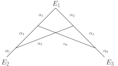
Figure 1: The “crossed-ladder” diagram with external vertices $E=\{E_{1}(x_{1}),E_{2}(x_{2}),E_{3}(x_{3})\}$.

Here we consider the $(x_{1}-x_{3})^{2}$ and $(x_{2}-x_{3})^{2}$ terms. The $(x_{1}-x_{2})^{2}$ term simply relates to $(x_{1}-x_{3})^{2}$ by symmetry. Direct calculation leads to

$$P_{13}(\alpha)=\frac{N_{13}(\alpha)}{D(\alpha)}\ ,$$ (71)

where the denominator

$$D(\alpha)= +\alpha_{1}\alpha_{2}\alpha_{3}\alpha_{4}+\alpha_{1}\alpha_{2}\alpha_{5}\alpha_{4}+\alpha_{1}\alpha_{3}\alpha_{5}\alpha_{4}+\alpha_{2}\alpha_{3}\alpha_{5}\alpha_{4}+\alpha_{1}\alpha_{3}\alpha_{6}\alpha_{4}+\alpha_{2}\alpha_{3}\alpha_{6}\alpha_{4}$$

$$+\alpha_{1}\alpha_{5}\alpha_{6}\alpha_{4}+\alpha_{2}\alpha_{5}\alpha_{6}\alpha_{4}+\alpha_{1}\alpha_{2}\alpha_{7}\alpha_{4}+\alpha_{2}\alpha_{3}\alpha_{7}\alpha_{4}+\alpha_{1}\alpha_{5}\alpha_{7}\alpha_{4}+\alpha_{3}\alpha_{5}\alpha_{7}\alpha_{4}$$

$$+\alpha_{1}\alpha_{6}\alpha_{7}\alpha_{4}+\alpha_{2}\alpha_{6}\alpha_{7}\alpha_{4}+\alpha_{3}\alpha_{6}\alpha_{7}\alpha_{4}+\alpha_{5}\alpha_{6}\alpha_{7}\alpha_{4}+\alpha_{1}\alpha_{3}\alpha_{8}\alpha_{4}+\alpha_{1}\alpha_{5}\alpha_{8}\alpha_{4}$$

$$+\alpha_{3}\alpha_{5}\alpha_{8}\alpha_{4}+\alpha_{3}\alpha_{6}\alpha_{8}\alpha_{4}+\alpha_{5}\alpha_{6}\alpha_{8}\alpha_{4}+\alpha_{1}\alpha_{7}\alpha_{8}\alpha_{4}+\alpha_{3}\alpha_{7}\alpha_{8}\alpha_{4}+\alpha_{6}\alpha_{7}\alpha_{8}\alpha_{4}$$

$$+\alpha_{1}\alpha_{2}\alpha_{3}\alpha_{6}+\alpha_{1}\alpha_{2}\alpha_{5}\alpha_{6}+\alpha_{1}\alpha_{3}\alpha_{5}\alpha_{6}+\alpha_{2}\alpha_{3}\alpha_{5}\alpha_{6}+\alpha_{1}\alpha_{2}\alpha_{6}\alpha_{7}+\alpha_{2}\alpha_{3}\alpha_{6}\alpha_{7}$$

$$+\alpha_{1}\alpha_{5}\alpha_{6}\alpha_{7}+\alpha_{3}\alpha_{5}\alpha_{6}\alpha_{7}+\alpha_{1}\alpha_{2}\alpha_{3}\alpha_{8}+\alpha_{1}\alpha_{2}\alpha_{5}\alpha_{8}+\alpha_{1}\alpha_{3}\alpha_{5}\alpha_{8}+\alpha_{2}\alpha_{3}\alpha_{5}\alpha_{8}$$

$$+\alpha_{2}\alpha_{3}\alpha_{6}\alpha_{8}+\alpha_{2}\alpha_{5}\alpha_{6}\alpha_{8}+\alpha_{3}\alpha_{5}\alpha_{6}\alpha_{8}+\alpha_{1}\alpha_{2}\alpha_{7}\alpha_{8}+\alpha_{2}\alpha_{3}\alpha_{7}\alpha_{8}+\alpha_{1}\alpha_{5}\alpha_{7}\alpha_{8}$$

$$+\alpha_{3}\alpha_{5}\alpha_{7}\alpha_{8}+\alpha_{2}\alpha_{6}\alpha_{7}\alpha_{8}+\alpha_{5}\alpha_{6}\alpha_{7}\alpha_{8}\ ,$$ (72)

sums over all the 45 spanning trees of the graph $G/(E_{1}\bigcup E_{2}\bigcup E_{3})$ shown in Fig. 2.

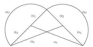
Figure 2: The contracted diagram $G/(E_{1}\bigcup E_{2}\bigcup E_{3})$.

On the other hand, one has

$$N_{13}(\alpha)= +\alpha_{1}\alpha_{2}\alpha_{3}\alpha_{4}\alpha_{8}+\alpha_{1}\alpha_{2}\alpha_{4}\alpha_{5}\alpha_{8}+\alpha_{1}\alpha_{3}\alpha_{4}\alpha_{5}\alpha_{8}+\alpha_{2}\alpha_{3}\alpha_{4}\alpha_{5}\alpha_{8}+\alpha_{1}\alpha_{2}\alpha_{3}\alpha_{6}\alpha_{8}$$

$$+\alpha_{1}\alpha_{3}\alpha_{4}\alpha_{6}\alpha_{8}+\alpha_{2}\alpha_{3}\alpha_{4}\alpha_{6}\alpha_{8}+\alpha_{1}\alpha_{2}\alpha_{5}\alpha_{6}\alpha_{8}+\alpha_{1}\alpha_{3}\alpha_{5}\alpha_{6}\alpha_{8}+\alpha_{2}\alpha_{3}\alpha_{5}\alpha_{6}\alpha_{8}$$

$$+\alpha_{1}\alpha_{4}\alpha_{5}\alpha_{6}\alpha_{8}+\alpha_{2}\alpha_{4}\alpha_{5}\alpha_{6}\alpha_{8}+\alpha_{1}\alpha_{2}\alpha_{4}\alpha_{7}\alpha_{8}+\alpha_{2}\alpha_{3}\alpha_{4}\alpha_{7}\alpha_{8}+\alpha_{1}\alpha_{2}\alpha_{6}\alpha_{7}\alpha_{8}$$

$$+\alpha_{1}\alpha_{4}\alpha_{6}\alpha_{7}\alpha_{8}+\alpha_{2}\alpha_{4}\alpha_{6}\alpha_{7}\alpha_{8}+\alpha_{1}\alpha_{5}\alpha_{6}\alpha_{7}\alpha_{8}\ .$$ (73)

The above can be decomposed according to ${\cal L}_{1}=\{\alpha_{2},\alpha_{4},\alpha_{8}\}$, ${\cal L}_{2}=\{\alpha_{1},\alpha_{6},\alpha_{8}\}$, ${\cal L}_{3}=\{\alpha_{1},\alpha_{3},\alpha_{4},\alpha_{5},\alpha_{8}\}$, ${\cal L}_{4}=\{\alpha_{2},\alpha_{3},\alpha_{5},\alpha_{6},\alpha_{8}\}$ as

$$N_{13}(\alpha)= +\alpha_{2}\alpha_{4}\alpha_{8}\bigg{(}\alpha_{1}\alpha_{3}+\alpha_{1}\alpha_{5}+\alpha_{1}\alpha_{7}+\alpha_{3}\alpha_{5}+\alpha_{3}\alpha_{6}+\alpha_{3}\alpha_{7}+\alpha_{5}\alpha_{6}+\alpha_{6}\alpha_{7}\bigg{)}$$

$$+\alpha_{1}\alpha_{6}\alpha_{8}\bigg{(}\alpha_{2}\alpha_{3}+\alpha_{2}\alpha_{5}+\alpha_{2}\alpha_{7}+\alpha_{3}\alpha_{4}+\alpha_{3}\alpha_{5}+\alpha_{4}\alpha_{5}+\alpha_{4}\alpha_{7}+\alpha_{5}\alpha_{7}\bigg{)}$$

$$+\alpha_{1}\alpha_{3}\alpha_{4}\alpha_{5}\alpha_{8}+\alpha_{2}\alpha_{3}\alpha_{5}\alpha_{6}\alpha_{8}\ .$$ (74)

The term $\alpha_{1}\alpha_{3}+\alpha_{1}\alpha_{5}+\alpha_{1}\alpha_{7}+\alpha_{3}\alpha_{5}+\alpha_{3}\alpha_{6}+\alpha_{3}\alpha_{7}+\alpha_{5}\alpha_{6}+\alpha_{6}\alpha_{7}$ sums over the spanning trees for $G/(E\bigcup{\cal L}_{1})$ and the term $\alpha_{2}\alpha_{3}+\alpha_{2}\alpha_{5}+\alpha_{2}\alpha_{7}+\alpha_{3}\alpha_{4}+\alpha_{3}\alpha_{5}+\alpha_{4}\alpha_{5}+\alpha_{4}\alpha_{7}+\alpha_{5}\alpha_{7}$ sums over the spanning trees for $G/(E\bigcup{\cal L}_{2})$. See Fig. 3 for depictions of these contracted diagrams.

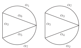
Figure 3: The contracted diagrams $G/(E\bigcup{\cal L}_{1}))$ (left) and $G/(E\bigcup{\cal L}_{2})$ (right).

Similarly, the $N_{23}$ term can be expressed as a sum over the connected paths $\{\alpha_{3},\alpha_{6},\alpha_{7},\alpha_{8}\}$ and $\{\alpha_{4},\alpha_{5},\alpha_{7},\alpha_{8}\}$

$$N_{23}(\alpha)=\alpha_{3}\alpha_{6}\alpha_{7}\alpha_{8}\bigg{(}\alpha_{2}+\alpha_{4}+\alpha_{5}\bigg{)}+\alpha_{4}\alpha_{5}\alpha_{7}\alpha_{8}\bigg{(}\alpha_{1}+\alpha_{3}+\alpha_{6}\bigg{)}\ .$$ (75)

It is easy to check that the corresponding sums $\alpha_{2}+\alpha_{4}+\alpha_{5}$ and $\alpha_{1}+\alpha_{3}+\alpha_{6}$ run over spanning trees for the corresponding contracted diagrams.

Appendix B Connecting ${\cal E}_{n}^{\prime}$ to ${\cal E}_{n}$ and path-connectedness of $\mathfrak{S}^{P}_{n}\bigcap{\cal E}^{\prime}_{n}$

To connect $\forall Z=(z_{n},z_{n-1},....z_{1})\in{\cal E}_{n}^{\prime}$ to ${\cal E}_{n}$, it is sufficient to chose the path $Z(s)|_{0\leq s\leq 1}=(z_{n}(s),z_{n-1}(s),..z_{1}(s))$ with $z_{i}(s)=i(y_{i}^{t},s\vec{y}_{i})+(sx_{i}^{t},\vec{x}_{i})$, namely, suppressing the imaginary spatial and real temporal components. Since ${\rm Re}(z_{ij}^{2}(s))=-(y_{i}^{t}-y_{j}^{t})^{2}-|\vec{x}_{i}-\vec{x}_{j}|^{2}+s^{2}(x_{i}^{t}-x_{j}^{t})^{2}+s^{2}|\vec{y}_{i}-\vec{y}_{j}|^{2}$, ${\rm Re}(z_{ij}^{2}(1))<0$ will guarantee that ${\rm Re}(z_{ij}^{2}(s))<0$ throughout $0\leq s\leq 1$, and clearly at $s=0$ the path reaches ${\cal E}_{n}$. Further notice that if $Z\in\mathfrak{S}_{n}^{P}$, then one also has $Z(s)\in\mathfrak{S}_{n}^{P}$ for the path above. Finally notice that $\mathfrak{S}^{P}_{n}\bigcap{\cal E}_{n}$ is path-connected. This shows the path-connectedness of $\mathfrak{S}^{P}_{n}\bigcap{\cal E}^{\prime}_{n}$ for any permutation $P$.

References

- Collins (2013) J. Collins, Foundations of perturbative QCD, Vol. 32 (Cambridge University Press, 2013).
- Diehl et al. (2016) M. Diehl, J. R. Gaunt, D. Ostermeier, P. Plößl, and A. Schäfer, JHEP 01, 076 (2016), arXiv:1510.08696 [hep-ph] .
- Ji (2013) X. Ji, Phys. Rev. Lett. 110, 262002 (2013), arXiv:1305.1539 [hep-ph] .
- Ji (2014) X. Ji, Sci. China Phys. Mech. Astron. 57, 1407 (2014), arXiv:1404.6680 [hep-ph] .
- Ji et al. (2021) X. Ji, Y.-S. Liu, Y. Liu, J.-H. Zhang, and Y. Zhao, Rev. Mod. Phys. 93, 035005 (2021), arXiv:2004.03543 [hep-ph] .
- Collins and Metz (2004) J. C. Collins and A. Metz, Phys. Rev. Lett. 93, 252001 (2004), arXiv:hep-ph/0408249 .
- Vladimirov (2016) A. Vladimirov, JHEP 12, 038 (2016), arXiv:1608.04920 [hep-ph] .
- Vladimirov (2018) A. Vladimirov, JHEP 04, 045 (2018), arXiv:1707.07606 [hep-ph] .
- Ji et al. (2020a) X. Ji, Y. Liu, and Y.-S. Liu, Nucl. Phys. B 955, 115054 (2020a), arXiv:1910.11415 [hep-ph] .
- Liu (2022) Y. Liu, Acta Phys. Polon. B 53, 4 (2022).
- Ji et al. (2020b) X. Ji, Y. Liu, and Y.-S. Liu, Phys. Lett. B 811, 135946 (2020b), arXiv:1911.03840 [hep-ph] .
- Ji and Liu (2022) X. Ji and Y. Liu, Phys. Rev. D 105, 076014 (2022), arXiv:2106.05310 [hep-ph] .
- Echevarria et al. (2016a) M. G. Echevarria, I. Scimemi, and A. Vladimirov, Phys. Rev. D 93, 011502 (2016a), [Erratum: Phys.Rev.D 94, 099904 (2016)], arXiv:1509.06392 [hep-ph] .
- Echevarria et al. (2016b) M. G. Echevarria, I. Scimemi, and A. Vladimirov, Phys. Rev. D 93, 054004 (2016b), arXiv:1511.05590 [hep-ph] .
- Li et al. (2020) Y. Li, D. Neill, and H. X. Zhu, Nucl. Phys. B 960, 115193 (2020), arXiv:1604.00392 [hep-ph] .
- Moult and Zhu (2018) I. Moult and H. X. Zhu, JHEP 08, 160 (2018), arXiv:1801.02627 [hep-ph] .
- Vladimirov (2020) A. A. Vladimirov, Phys. Rev. Lett. 125, 192002 (2020), arXiv:2003.02288 [hep-ph] .
- Streater and Wightman (1989) R. F. Streater and A. S. Wightman, PCT, spin and statistics, and all that (1989).
- Jost (1965) R. Jost, The general theory of quantized fields, Vol. 4 (American Mathematical Society, Providence, RI, 1965).
- Osterwalder and Schrader (1973) K. Osterwalder and R. Schrader, Commun. Math. Phys. 31, 83 (1973).
- Osterwalder and Schrader (1975) K. Osterwalder and R. Schrader, Commun. Math. Phys. 42, 281 (1975).
- Wu et al. (1976) T. T. Wu, B. M. McCoy, C. A. Tracy, and E. Barouch, Phys. Rev. B 13, 316 (1976).
- McCoy et al. (1977) B. M. McCoy, C. A. Tracy, and T. T. Wu, Phys. Rev. Lett. 38, 793 (1977).
- Feldman et al. (1985) J. Feldman, J. Magnen, V. Rivasseau, and R. Seneor, Phys. Rev. Lett. 54, 1479 (1985).
- Feldman et al. (1986) J. Feldman, J. Magnen, V. Rivasseau, and R. Seneor, Commun. Math. Phys. 103, 67 (1986).
- Luscher and Mack (1975) M. Luscher and G. Mack, Commun. Math. Phys. 41, 203 (1975).
- Hartman et al. (2016) T. Hartman, S. Jain, and S. Kundu, JHEP 05, 099 (2016), arXiv:1509.00014 [hep-th] .
- Caron-Huot (2017) S. Caron-Huot, JHEP 09, 078 (2017), arXiv:1703.00278 [hep-th] .
- Caron-Huot and Sandor (2021) S. Caron-Huot and J. Sandor, JHEP 05, 059 (2021), arXiv:2008.11759 [hep-th] .
- Ji et al. (2023) X. Ji, Y. Liu, and Y. Su, JHEP 08, 037 (2023), arXiv:2305.04416 [hep-ph] .
- Bogner and Weinzierl (2010) C. Bogner and S. Weinzierl, Int. J. Mod. Phys. A 25, 2585 (2010), arXiv:1002.3458 [hep-ph] .
- Kugo and Ojima (1979) T. Kugo and I. Ojima, Prog. Theor. Phys. Suppl. 66, 1 (1979).
- Korchemskaya and Korchemsky (1992) I. A. Korchemskaya and G. P. Korchemsky, Phys. Lett. B 287, 169 (1992).
- Korchemsky and Marchesini (1993) G. P. Korchemsky and G. Marchesini, Nucl. Phys. B 406, 225 (1993), arXiv:hep-ph/9210281 .
- Vladimirov (2017) A. A. Vladimirov, Phys. Rev. Lett. 118, 062001 (2017), arXiv:1610.05791 [hep-ph] .
- Collins (2008) J. Collins, PoS LC2008, 028 (2008), arXiv:0808.2665 [hep-ph] .
- Ji et al. (2019) X. Ji, L.-C. Jin, F. Yuan, J.-H. Zhang, and Y. Zhao, Phys. Rev. D 99, 114006 (2019), arXiv:1801.05930 [hep-ph] .
- Aglietti (1994) U. Aglietti, Nucl. Phys. B 421, 191 (1994), arXiv:hep-ph/9304274 .
- Hashimoto and Matsufuru (1996) S. Hashimoto and H. Matsufuru, Phys. Rev. D 54, 4578 (1996), arXiv:hep-lat/9511027 .
- Horgan et al. (2009) R. R. Horgan et al., Phys. Rev. D 80, 074505 (2009), arXiv:0906.0945 [hep-lat] .
- Collins (2018) J. Collins, (2018), arXiv:1801.03960 [hep-ph] .