Hacking Task Confounder in Meta-Learning

Abstract

Meta-learning enables rapid generalization to new tasks by learning meta-knowledge from a variety of tasks. It is intuitively assumed that the more tasks a model learns in one training batch, the richer knowledge it acquires, leading to better generalization performance. However, contrary to this intuition, our experiments reveal an unexpected result: adding more tasks within a single batch actually degrades the generalization performance. To explain this unexpected phenomenon, we conduct a Structural Causal Model (SCM) for causal analysis. Our investigation uncovers the presence of spurious correlations between task-specific causal factors and labels in meta-learning. Furthermore, the confounding factors differ across different batches. We refer to these confounding factors as “Task Confounders”. Based on this insight, we propose a plug-and-play Meta-learning Causal Representation Learner (MetaCRL) to eliminate task confounders. It encodes decoupled causal factors from multiple tasks and utilizes an invariant-based bi-level optimization mechanism to ensure their causality for meta-learning. Extensive experiments on various benchmark datasets demonstrate that our work achieves state-of-the-art (SOTA) performance.

Introduction

Meta-learning aims to develop algorithms capable of adapting to previously unseen tasks. To achieve this goal, meta-learning methods are trained on a diverse set of tasks, enabling them to learn meta-knowledge that can be applied to new and related tasks. Moreover, meta-learning has been demonstrated to address numerous inherent challenges in deep learning, such as computational bottlenecks and generalization issues (Du et al. 2020; Li et al. 2018). It is widely used in domains like reinforcement learning (Mitchell et al. 2021), computer vision (Mahadevkar et al. 2022), and robotics (Schrum et al. 2022).

In general, meta-learning can be defined as a bi-level optimization process. In the inner loop, task-specific parameters are independently learned based on meta-parameters. In the outer loop, the meta-parameters are updated by minimizing the average loss across multiple tasks using the learned task-specific parameters. During the meta-training process, each batch’s training set consists of a series of randomly sampled different tasks, with each task containing training samples from various categories. By leveraging shared structures across multiple tasks, the meta-learning model can acquire rich meta-knowledge, leading to great generalization and adaptation (Wang, Zhao, and Li 2021; Song et al. 2022). Therefore, a widely adopted hypothesis is that the more tasks the model learns in a single training batch, the richer knowledge it acquires, and consequently, the better its performance will be (Hospedales et al. 2021; Rivolli et al. 2022). This idea is intuitively reasonable since learning from a broader range of scenarios can help grasp a wealth of knowledge, resembling human cognition.

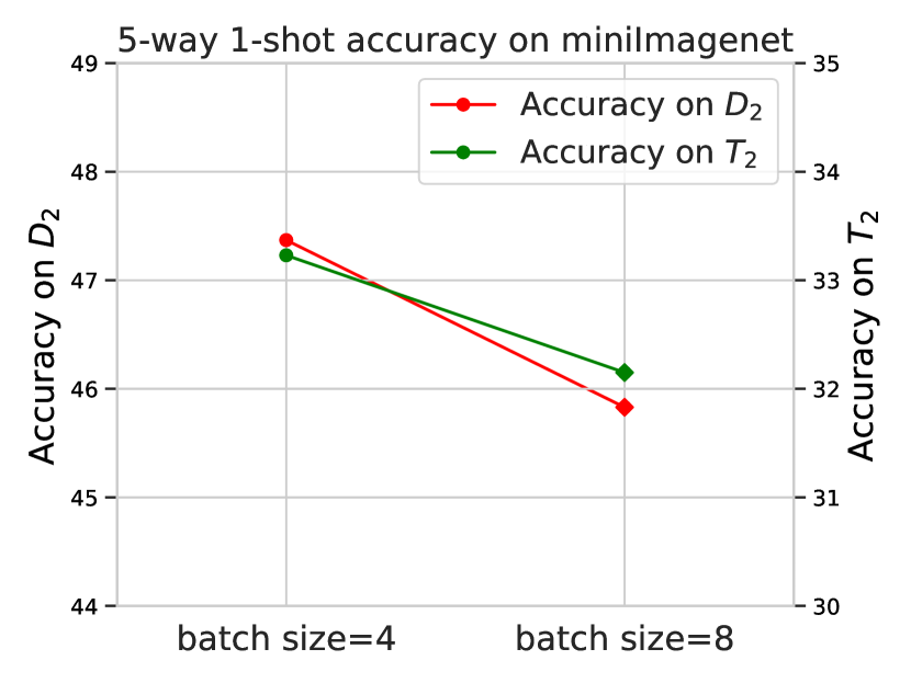
(a) miniImagenet

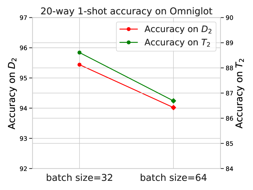
(b) Omniglot

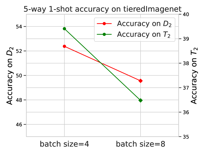
(c) tieredImagenet

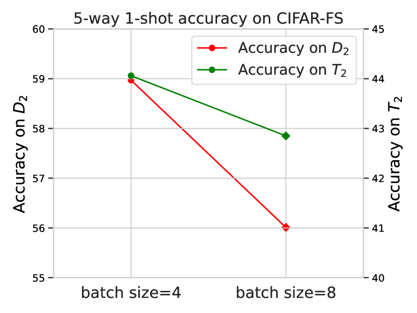
(d) CIFAR-FS

Figure 1: The empirical results on four benchmark datasets.

However, our experiments yield conflicting results. We sample two sets of non-overlapping tasks, $\mathcal{T}_{1}$ and $\mathcal{T}_{2}$. Within $\mathcal{T}_{1}$, we divide the tasks into a meta-training set $\mathcal{D}_{1}$ and a meta-testing set $\mathcal{D}_{2}$, while $\mathcal{T}_{2}$ is used solely for separate testing without being split. We train MAML (Finn, Abbeel, and Levine 2017) on $\mathcal{D}_{1}$ with two different batch size settings, i.e., batch size=$B$ and batch size=$2B$. Then we test it on $\mathcal{D}_{2}$ and $\mathcal{T}_{2}$. Intuitively, the model with a larger batch size is expected to perform better. Surprisingly, as shown in Figure 1, when batch size=$2B$, the model exhibits lower accuracy on both $\mathcal{D}_{2}$ and $\mathcal{T}_{2}$ across all four benchmark datasets.

To explore the causes of this phenomenon, we construct a Structural Causal Model (SCM). As shown in Figure 2(b), we denote the distinct causal factors of task $\tau_{i}$ and task $\tau_{j}$ as ${\rm{A}}^{i}$ and ${\rm{A}}^{j}$, as well as the shared causal factors as ${\rm{B}}^{i,j}$. To ensure a generic prior that performs well, meta-learning performs joint learning on all tasks. Thus, the non-overlapping causal factors ${\rm{A}}^{i}$ of $\tau_{i}$ may cause spurious correlations with $\tau_{j}$, and ${\rm{A}}^{j}$ holds the same with $\tau_{i}$. This misleading correlation introduces bias into meta-knowledge, ultimately affecting model generalization. Additionally, it varies across different batches, e.g., the tasks differ in different batches. We identify this confounding factor as “Task Confounder”.

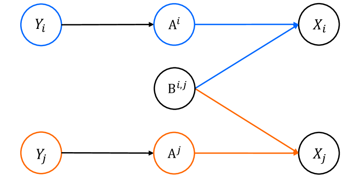
(a) data generation mechanism

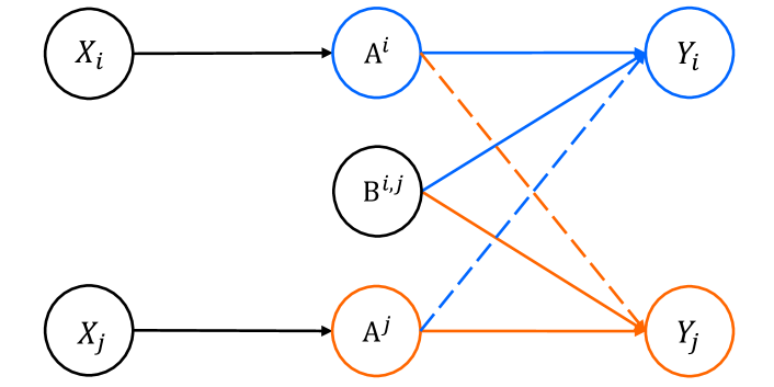
(b) meta-learning process in practice

Figure 2: The Structural Causal Model (SCM) regarding two tasks $\tau_{i}$ and $\tau_{j}$, where $(X_{i},Y_{i})$ and $(X_{j},Y_{j})$ are the samples and corresponding labels of these two tasks. The solid line means the causal correlation, and the dotted line means the spurious correlation. (a) is constructed based on the ground-truth causal mechanism, while (b) can be viewed as the inverse process of the generating mechanism.

Inspired by this insight, we propose a plug-and-play meta-learning causal representation learner (MetaCRL) to encode decoupled causal knowledge, thereby eliminating task confounders. It consists of two modules: the disentangling module and the causal module. The former aims to extract causal factors across all tasks and provide a subset of causal factors relevant to each task, while the latter is responsible for ensuring their causality. The modules achieve their objectives through a simple bi-level optimization mechanism with regularization terms. By incorporating MetaCRL into meta-learning, we dynamically eliminate task confounders during the training process. Through extensive evaluations on multiple meta-learning benchmarks, we demonstrate that MetaCRL can significantly improve performance.

Our contributions are as follows: (i) We discover a counterintuitive phenomenon: by increasing the batch size during meta-training, the model’s generalization becomes worse; (ii) We construct an SCM to analyze the phenomenon, finding spurious correlations, named “Task Confounders”, between non-shared features of training tasks and the generic label space of meta-learning; (iii) We propose MetaCRL, a plug-and-play meta-learning causal representation learner, effectively eliminating the task confounders and improving generalization performance; (iv) Extensive empirical analysis showcases the outstanding performance of MetaCRL.

Related Work

Meta-learning aims to construct tasks and learn from them using limited data, thus generalizing to new tasks based on the acquired knowledge. Typical methods can be categorized into two types: optimization-based (Finn, Abbeel, and Levine 2017; Nichol and Schulman 2018; Raghu et al. 2019) and metric-based (Snell, Swersky, and Zemel 2017; Sung et al. 2018; Chen et al. 2020) approaches. They both rely on shared structures to extract meta-knowledge, resulting in remarkable performance on new tasks. However, meta-learning still faces the crisis of performance degradation. Various approaches have been proposed to address this issue, such as adding adaptive noise(Lee et al. 2020), reducing inter-task disparities(Jamal and Qi 2019), limiting the trainable parameters(Yin et al. 2019; Oh et al. 2020), and task augmentation(Yao et al. 2021). These methods overlook the influence between tasks during the training process, which is shown to be crucial in the motivation section. In this study, we focus on the fundamental causes of performance degradation in meta-training tasks and attempt to find a general method to address this problem.

Causal learning is an important branch of machine learning, aiming to understand and infer causal relationships between events. It models the target with a directed acyclic graph and helps in optimizing the model by eliminating confounders in the causal graph. Recent studies (Yang, Zhang, and Cai 2021; Zhang et al. 2020; Nogueira et al. 2022) have already shown that it aids deep learning models in unearthing underlying causal factors. Current research attempts to combine causal knowledge with meta-learning methods to address domain challenges. Yue et al. (Yue et al. 2020) removed performance limitations of pre-trained knowledge through backdoor regulation. Ton et al. (Ton, Sejdinovic, and Fukumizu 2021) utilized causal knowledge to distinguish causes and effects in a bivariate environment with limited data. Jiang et al. (Jiang et al. 2022) used causal graphs to remove undesirable memory effects. While they all combine meta-learning and causal learning, their focus is on addressing problems that differ significantly from ours.

Problem Formulation and Analysis

Notation and Problem Definition

Given a task distribution $p(\mathcal{T})$, the meta-training set $\mathcal{D}_{tr}$ and the meta-testing set $\mathcal{D}_{te}$ are all sampled from $p(\mathcal{T})$ without any class-level overlap. We denote the $N_{tr}$ tasks in a single training batch as $\left\{\tau_{i}\right\}_{i=1}^{N_{tr}}\in\mathcal{D}_{tr}$. Each task $\tau_{i}$ consists of a support set $\mathcal{D}_{i}^{s}=(X_{i}^{s},Y_{i}^{s})=\{(x_{i,j}^{s},y_{i,j}^{s})\}_{j=1}^{N_{i}^{s}}$ and a query set $\mathcal{D}_{i}^{q}=(X_{i}^{q},Y_{i}^{q})=\{(x_{i,j}^{q},y_{i,j}^{q})\}_{j=1}^{N_{i}^{q}}$, where $(x_{i,j}^{\cdot},y_{i,j}^{\cdot})$ represents the sample and the corresponding label, and $N_{i}^{\cdot}$ denotes the number of the samples. Meta-learning utilizes the shared encoder $g$ and the classifier $h$ to learn the above tasks. For simplicity, we denote the meta-learning model as $f_{\theta}=h\circ g$ with the meta-parameter $\theta$ to be learned. Note that the optimal $f_{\theta}$ can serve as general initial priors to help task-specific models adapt quickly to new tasks.

Following (Gordon et al. 2018; Jiang et al. 2022), the objective of meta-learning can be formulated as maximizing the conditional likelihood $\sum\nolimits_{i}{p(Y_{i}^{q}|X_{i}^{q},{\cal D}_{i}^{s},{f_{\theta}})}$. This can be viewed as a bi-level optimization process. In this context, the inner-loop optimizes $p(Y_{i}^{s}|X_{i}^{s},f_{\theta})$ for learning the $i$-th task-specific model $f^{i}_{\theta}$, which can be presented as:

$$\begin{array}[]{l}\qquad\qquad f^{i}_{\theta}\leftarrow f_{\theta}-\alpha\nabla_{f_{\theta}}\mathcal{L}(Y_{i}^{s},X_{i}^{s},f_{\theta})\\[5.0pt] s.t.\quad\mathcal{L}(Y_{i}^{s},X_{i}^{s},f_{\theta})=\frac{1}{N_{i}^{s}}\sum_{j=1}^{N_{i}^{s}}y_{i,j}^{s}\log{f_{\theta}}(x_{i,j}^{s})\end{array}$$ (1)

where $\alpha$ is the learning rate. The outer loop optimizes $\sum\nolimits_{i}{p(Y_{i}^{q}|X_{i}^{q},f_{\theta}^{i},{f_{\theta}})}$ for learning $f_{\theta}$, which can be presented as:

$$\begin{array}[]{l}\qquad f_{\theta}\leftarrow f_{\theta}-\beta\nabla_{f_{\theta}}\frac{1}{N_{tr}}\sum_{i=1}^{N_{tr}}\mathcal{L}(Y_{i}^{q},X_{i}^{q},f_{\theta}^{i})\\[5.0pt] s.t.\quad\mathcal{L}(Y_{i}^{q},X_{i}^{q},f_{\theta}^{i})=\frac{1}{N_{i}^{q}}\sum_{j=1}^{N_{i}^{q}}y_{i,j}^{q}\log{f_{\theta}^{i}}(x_{i,j}^{q})\end{array}$$ (2)

where $\beta$ is the learning rate. It is worth noting that $f_{\theta}^{i}$ is obtained by taking the derivative of $f_{\theta}$, so $f_{\theta}^{i}$ can be regarded as a function of $f_{\theta}$. Therefore, $\nabla_{f_{\theta}}\frac{1}{N_{tr}}\sum_{i=1}^{N_{tr}}\mathcal{L}(Y_{i}^{q},X_{i}^{q},f_{\theta}^{i})$ can be viewed as the second derivative of $f_{\theta}$.

Empirical Evidence

According to Eq. 1 and Eq. 2, we can conclude that meta-learning can be viewed as a multi-task learning process. Meanwhile, a well-generalized meta-learning model encodes the label-related factors for all tasks to obtain rich knowledge. Therefore, intuitively, one might assume that increasing the batch size would enhance the performance. However, our experiments show that this is not always true.

In our empirical evaluation, we begin by sampling a collection of tasks, denoted as $\mathcal{T}_{1}=\left\{\tau_{i}\right\}_{i=1}^{N_{1}}$. Subsequently, we partition the sample sets of all tasks within $\mathcal{T}_{1}$ into two distinct subsets: one allocated for training, denoted as $\mathcal{D}_{1}$, and the other designated for testing, denoted as $\mathcal{D}_{2}$. Following this, we proceed to sample a new task collection $\mathcal{T}_{2}=\left\{\tau_{i}\right\}_{i=1}^{N_{2}}$, ensuring that the tasks do not overlap with $\mathcal{T}_{1}$. We establish MAML as our baseline method and select miniImagenet (Vinyals et al. 2016), Omniglot (Lake, Salakhutdinov, and Tenenbaum 2019), tieredImagenet (Ren et al. 2018) and CIFAR-FS (Bertinetto et al. 2018) as benchmark datasets. During the training phase, we utilize two different batch size settings on $\mathcal{D}_{1}$ to train MAML, i.e., batch size=$B$ and batch size=$2B$, where $B$ represents the commonly used setting on the corresponding dataset, e.g., $B=4$ for miniImagenet and $B=32$ for Omniglot. Subsequently, we evaluate the trained models on $\mathcal{D}_{2}$ and $\mathcal{T}_{2}$, respectively.

Some abnormal outcomes are summarized in Figure 1 (see appendix for full results). Our observations reveal the following: (i) Increasing the number of tasks per batch during training leads to a decrease in test accuracy on $\mathcal{D}_{2}$. It indicates that simply increasing the task quantity does not guarantee an improvement in the model’s performance on the current tasks. Furthermore, this observation suggests that the synergistic enhancement between different tasks is not always evident; in fact, instances of task confounders, where different tasks inhibit each other, may also manifest. (ii) The test accuracy on $\mathcal{T}{2}$ also decreases when the number of tasks per batch during training is increased. In conjunction with observation (i), it becomes evident that the generalization of the meta-learning model is suppressed when there are task confounders among multiple tasks.

Causal Analysis and Motivation

To explore the reasons behind the task confounders mentioned above, we construct an SCM for meta-learning regarding two tasks $\tau_{i}$ and $\tau_{j}$ based on data generation mechanisms, as illustrated in Figure 2(a). In this model, $Y_{i}$ and $Y_{j}$ denote the label variables for tasks $\tau_{i}$ and $\tau_{j}$ respectively, while $X_{i}$ and $X_{j}$ signify the sample variables for the two tasks, respectively. Additionally, ${{\rm A}^{i}}$ and ${{\rm A}^{j}}$ represent distinct sets of causal factors exclusive to tasks $\tau_{i}$ and $\tau_{j}$, respectively, such as color, shape, and texture. On the other hand, ${{\rm B}^{i,j}}$ encompasses causal factors shared between tasks $\tau_{i}$ and $\tau_{j}$. We assume that the samples and the labels are both generated by a ground-truth causal mechanism following (Suter et al. 2019; Hu et al. 2022). Specifically, we assume that the sample is generated by disentangled causal mechanisms, e.g., $p({X_{i}}|{{\rm A}^{i}},{{\rm{B}}^{i,j}})=\prod\nolimits_{k}{p({X_{i}}|{{\rm A}^{i}_{k}})}\prod\nolimits_{t}{p({X_{i}}|{\rm B}_{t}^{i,j})}$, where ${\rm A}^{i}_{k}$ denotes the $k$-th element of ${\rm A}^{i}$ and ${\rm B}_{t}^{i,j}$ denotes the $t$-th element of ${\rm B}^{i,j}$. As ${\rm A}^{i}$, ${\rm A}^{j}$, and ${\rm B}^{i,j}$ represent high-level knowledge of the data, we could naturally define the task label variable $Y_{i}$ for task $i$ as the cause of the ${\rm B}^{i,j}$ and ${\rm A}^{i}$. For the task $\tau_{i}$, we call ${\rm B}^{i,j}$ and ${\rm A}^{i}$ as the causal feature variables that are causally related to $Y_{i}$, and we call ${\rm A}^{j}$ as the non-causal feature variables to task $\tau_{i}$. Therefore, we have $p({X_{i}}|{{\rm A}^{i}},{{\rm{B}}^{i,j}},{{\rm A}^{j}})=p({X_{i}}|{{\rm A}^{i}},{{\rm{B}}^{i,j}})$.

Based on the proposed SCM, an ideal meta-learning predictor for each task should only utilize causal factors and be invariant to any intervention on non-causal factors. However, the joint learning of multiple tasks can give rise to the issue of spurious correlations, thereby making it challenging to achieve optimal predictions. In order to investigate the mechanisms underlying the generation of spurious correlations, we consider the scenario of two binary classification tasks. Let $Y_{i}$ and $Y_{j}$ be variables from $\left\{{\pm 1}\right\}$. We assume the two tasks have non-overlapping factors, e.g., ${{\rm{B}}^{i,j}}=\emptyset$, and the elements in ${{\rm A}^{i}}$ and ${{\rm A}^{j}}$ satisfy the constraint of Gaussian distribution. Then, we have:

Theorem 1

If the correlation between $Y_{i}$ and $Y_{j}$ is not equal to 0.5, the optimal classifier has non-zero weights for non-causal factors for each task. If the correlation between $Y_{i}$ and $Y_{j}$ equals 0.5 and the number of training samples is limited, the optimal classifier also has non-zero weights for non-causal factors for each task.

As inferred from the aforementioned theorem, the learned model leverages the causal factors from other tasks to facilitate the learning of the target task. The SCM corresponding to this process is illustrated in Figure 2(b). Taking the task $\tau_{i}$ as an example, the meta-learning model uses the causal factors ${{\rm A}^{j}}$ belonging to the task $\tau_{j}$ for learning $Y_{i}$. Thus, there is a spurious correlation between ${{\rm A}^{j}}$ and $Y_{i}$, which can be represented as a spurious path ${{\rm A}^{j}}\to Y_{i}$. Also, we can obtain the spurious path ${{\rm A}^{i}}\to Y_{j}$. The learning process can be viewed as the inverse process of the generating mechanism. Therefore, we can obtain the SCM with two spurious paths, which can reflect the internal mechanism of task confounders in multi-task learning. The proof of Theorem 1 is provided in Appendix A.

Methodology

Based on the above evidence and analysis, we can know that task confounders can cause spurious correlations between causal factors and labels. An ideal meta-learning model should learn multi-task knowledge in a shared representation and identify which portions of knowledge are causally related to each task. This inspires us to propose a method called MetaCRL that can encode decoupled causal knowledge. It serves as a plug-and-play learner that consists of two modules: the disentangling module and the causal module. The disentangling module aims to acquire all causal factors and provide subsets of causal factors specifically relevant to individual tasks, while the causal module aims to ensure the causality of factors in the disentangling module. The pseudocode of our MetaCRL is provided in Appendix B.

Disentangling Module

For a pre-trained CNN-based encoder, each channel can be regarded as being related to a kind of semantic information or visual concept (Islam, Jia, and Bruce 2020). Thus, we can use the data representation to learn the causal factors. During the training phase, we denote the $N_{tr}$ training tasks as $\left\{\tau_{i}\right\}_{i=1}^{N_{tr}}$. Suppose that the number of causal factors is $N_{k}$, then, we propose obtaining these $N_{k}$ factors through the learning of a matrix $\Xi\in{{\mathbb{R}}^{N_{z}\times N_{k}}}$, where $N_{z}$ represents the dimension of the feature representation, e.g., the output dimension of the encoder $g$, and each column of $\Xi$ represents a distinct factor. Based on $\Xi$, we can obtain a new representation of each sample, which can be called a causal representation, e.g., the causal representation for $x_{i,j}^{s}$ can be presented as ${\Xi^{\rm{T}}}g(x_{i,j}^{s})$. Based on the causal analysis above, the causal factors should be divided into $N_{tr}$ overlapping groups, and each group corresponds to a task. To obtain these groups, we propose a learnable grouping function $f_{gr}$, which is implemented using Multi-Layer Perceptrons (MLPs). Specifically, for task $\tau_{i}$, we first calculate the average sample $x_{i}$ for this task, e.g., ${x_{i}}=\frac{1}{N_{i}^{s}+N_{i}^{q}}(\sum\nolimits_{j=1}^{N_{i}^{s}}{x_{i,j}^{s}}+\sum\nolimits_{j=1}^{N_{i}^{q}}{x_{i,j}^{q}})$. Subsequently, $x_{i}$ is input into $g$, $\Xi$, and $f_{gr}$, e.g., ${f_{gr}}({\Xi^{\rm{T}}}g({x_{i}}))$, yielding a vector with all elements greater than zero and matching the dimensionality of the causal representation. Concurrently, each element is subject to the normalization operation $\rm{Norm}$. As a result, the individual elements of the output vector ${\rm{Norm}}(f_{gr})$ can be interpreted as the probabilities that each causal factor belongs to $\tau_{i}$. In a word, we can obtain the causal factors for each task based on $\tau_{i}$ and $f_{gr}$.

Ideally, each factor in $\Xi$ should represent a distinct semantic, and changing one factor should not affect others. However, in reality, without explicit constraints, the factors in $\Xi$ may still be correlated, hindering the learning of causal structures (Locatello et al. 2019). Therefore, we propose a regularization term to achieve complete decoupling. Specifically, we directly penalize the similarity between different factors, which can be formulated as:

$$\mathcal{L}_{\rm{DM}}(\Xi)=\sum\limits_{i=1}^{{N_{k}}-1}\sum\limits_{j=i+1}^{N_{k}}{\Xi_{:,i}^{\rm{T}}{\Xi_{:,j}}}$$ (3)

where ${{\Xi_{:,i}}}$ represents the $i$-th column of $\Xi$. As we can see, minimizing $\mathcal{L}_{\rm{DM}}(\Xi)$ can lead to a similarity of 0 between different causal factors, thereby empirically establishing independence among distinct factors.

Note that each task is only related to a small number of factors, and the factors of different tasks can vary greatly. It may lead to degenerate solutions in which only a few factors are utilized. Therefore, we need to constrain the output of $f_{gr}$ to be sparse and diverse. To achieve this, we propose to use the $L_{1}$ norm with an entropy term to the output of $f_{gr}$:

$$\begin{array}[]{l}\mathcal{L}_{\rm{DM}}(f_{gr})=\sum\limits_{i=1}^{{N_{tr}}}{{{\left\|{{f_{gr}}({\Xi^{\rm{T}}}g({x_{i}}))}\right\|}_{1}}}\\ \quad\quad\quad\quad\quad\quad-{\rm{Entropy}}(\frac{{\sum\nolimits_{j}{{f_{gr}}{{({\Xi^{\rm{T}}}g({x_{i}}))}_{j}}}}}{{\sum\nolimits_{i}{\sum\nolimits_{j}{{f_{gr}}{{({\Xi^{\rm{T}}}g({x_{i}}))}_{j}}}}}})\end{array}$$ (4)

where ${{f_{gr}}{{({\Xi^{\rm{T}}}g({x_{i}}))}_{j}}}$ represents the $j$-th element of the output of $f_{gr}$. We can see that minimizing the first term of $\mathcal{L}_{\rm{DM}}(f_{gr})$ can make the output of $f_{gr}$ to be sparse, and maximizing the second term of $\mathcal{L}_{\rm{DM}}(f_{gr})$ can make the output of $f_{gr}$ to be diverse.

By combining Eq.3 and Eq.4, the loss of the disentangling module can be presented as:

$$\mathcal{L}_{\rm{DM}}(f_{gr},\Xi)=\lambda_{1}\cdot\mathcal{L}_{\rm{DM}}(\Xi)+\lambda_{2}\cdot\mathcal{L}_{\rm{DM}}(f_{gr})$$ (5)

where $\lambda_{1}$ and $\lambda_{2}$ denote the loss weights of $\mathcal{L}_{\rm{DM}}(\Xi)$ and $\mathcal{L}_{\rm{DM}}(f_{gr})$, respectively.

Causal Module

In the disentangling module, each column of $\Xi$ is treated as a causal factor. However, due to the random initialization of matrix $\Xi$ and the absence of explicit constraints in the disentangling module, ensuring causality in $\Xi$ becomes challenging. Moreover, the causal factors for each task also exhibit randomness, making it difficult to guarantee their authenticity. To solve these problems, we propose the causal module to ensure causality in the disentangling module. Following (Koyama and Yamaguchi 2020), we can see that a model invariant to multiple distributions could learn causal correlations. Also, based on Theorem 9 described in (Arjovsky et al. 2019), by enforcing invariance over multiple training datasets that exhibit distribution shifts, the task-specific models should only utilize causal factors that are helpful to themselves, and assign zero weights to those non-causal factors for the task. Therefore, the causal module is designed to facilitate causal learning by using this invariance.

As widely known, during the training phase of meta-learning, the training data can be divided into multiple support sets and multiple query sets. As they comprise different samples, they can be regarded as distinct data distributions with distributional shifts. Meanwhile, the learning process in Eq.2 can be depicted as follows: First, for every $f_{\theta}$, optimizing Eq. 1 can achieve an optimal $f_{\theta}^{i}$ and $\mathcal{L}(Y_{i}^{s},X_{i}^{s},f_{\theta}^{i})$ on the support set. Subsequently, altering the value of $f_{\theta}$ impacts the optimal $f_{\theta}^{i}$ accordingly. At last, seek the optimal $f_{\theta}$ to obtain the optimal $f_{\theta}^{i}$ that can optimize $\frac{1}{N_{tr}}\sum_{i=1}^{N_{tr}}\mathcal{L}(Y_{i}^{q},X_{i}^{q},f_{\theta}^{i})$ on the query set. Consequently, the optimization of Eq.1 and Eq.2 can be interpreted as achieving optimality across multiple datasets using the same $f_{\theta}$. Based on the above illustration, we propose to utilize a bi-level optimization mechanism to learn $\Xi$ and $f_{gr}$, e.g., similar to Eq.1 and Eq.2, thus ensuring causality. Specifically, for the first level, we learn $\Xi^{{}^{\prime}}$ and ${f}_{gr}^{{}^{\prime}}$ with the support sets through the following objectives:

$$\begin{array}[]{l}\qquad\qquad\qquad\left\{\begin{matrix}\Xi^{{}^{\prime}}\leftarrow\Xi-\alpha_{1}{\nabla_{\Xi}}\tilde{\mathcal{L}}\\ f_{gr}^{{}^{\prime}}\leftarrow{f}_{gr}-\alpha_{2}{\nabla_{{f_{gr}}}}\tilde{\mathcal{L}}\end{matrix}\right.\\[15.0pt] s.t.\quad\tilde{\mathcal{L}}=\frac{1}{N_{tr}}\sum_{i=1}^{N_{tr}}{\mathcal{L}(Y_{i}^{s},X_{i}^{s},\Xi,{{f}_{gr}})}+{\mathcal{L}_{{\rm{DM}}}}(\Xi,{{f}_{gr}})\\[8.0pt] \qquad\mathcal{L}(Y_{i}^{s},X_{i}^{s},\Xi,f_{gr})=\frac{1}{{N_{i}^{s}}}\sum\nolimits_{j=1}^{N_{i}^{s}}y_{i,j}^{s}\log\mathrm{z}_{i,j}^{s}\\[8.0pt] \qquad\mathrm{z}_{i,j}^{s}=h\{{\rm{Norm[}}{f_{gr}}({\Xi^{\rm{T}}}g({x_{i}}))]\odot[{\Xi^{\rm{T}}}g(x_{i,j}^{s})]\}\end{array}$$ (6)

and for the second level, we learn ${\Xi}$ and ${{f}_{gr}}$ with the query sets through the following objectives:

$$\begin{array}[]{l}\qquad\qquad\qquad\left\{\begin{matrix}\Xi\leftarrow\Xi-\alpha_{3}{\nabla_{\Xi}}\tilde{\mathcal{L}^{{}^{\prime}}}\\ {f_{gr}}\leftarrow{{f}_{gr}}-\alpha_{4}{\nabla_{{f_{gr}}}}\tilde{\mathcal{L}^{{}^{\prime}}}\end{matrix}\right.\\[15.0pt] s.t.\quad\tilde{\mathcal{L}^{{}^{\prime}}}=\frac{1}{N_{tr}}\sum_{i=1}^{N_{tr}}{\mathcal{L}(Y_{i}^{q},X_{i}^{q},\Xi^{{}^{\prime}},f_{gr}^{{}^{\prime}})}+{\mathcal{L}_{{\rm{DM}}}}(\Xi^{{}^{\prime}},f_{gr}^{{}^{\prime}})\\[8.0pt] \qquad\mathcal{L}(Y_{i}^{q},X_{i}^{q},\Xi^{{}^{\prime}},f_{gr}^{{}^{\prime}})=\frac{1}{{N_{i}^{q}}}\sum\nolimits_{j=1}^{N_{i}^{q}}y_{i,j}^{q}\log\mathrm{z}_{i,j}^{q}\\[8.0pt] \qquad\mathrm{z}_{i,j}^{q}=h\{{\rm{Norm[}}{f_{gr}}({{\Xi^{{}^{\prime}}}^{\rm{T}}}g({x_{i}}))]\odot[{{\Xi^{{}^{\prime}}}^{\rm{T}}}g(x_{i,j}^{q})]\}\end{array}$$ (7)

where $\odot$ represents the element-wise multiplication operator between two vectors, while $\alpha_{1}$, $\alpha_{2}$, $\alpha_{3}$ and $\alpha_{4}$ are the learning rates. It’s worth noting that $\mathcal{L}(Y_{i}^{\cdot},X_{i}^{\cdot},\Xi,{f_{gr}})$ is optimized using the causal representation ${\Xi^{\rm{T}}}g(x_{i,j}^{\cdot})$ with the weight ${\rm{Norm[}}{f_{gr}}({\Xi^{\rm{T}}}g({x_{i}}))]$. The weight is intended to restrict the causal features of samples in the task $\tau_{i}$ to be associated only with a subset of causal factors.

The learning process of $\Xi$ and $f_{gr}$ can be regarded as enforcing invariance over the support sets and the query sets, thus, the bi-level optimization mechanism for $\Xi$ and $f_{gr}$ can ensure causality. Meanwhile, Eq.6 and Eq.7 are learned based on pre-defined $h$ and $g$, thus rendering the MetaCRL a plug-and-play learner.

Overall Objective

In this subsection, we embed the above causal representation learning process into a meta-learning framework for joint optimization. The training process for MetaCRL in each batch is divided into two steps. In the first step, with $\Xi$ and $f_{gr}$ held fixed, we optimize $h$ and $g$. Specifically, the objective of the inner loop mentioned in Eq.1 becomes:

$$\begin{array}[]{l}\qquad f^{i}_{\theta}\leftarrow f_{\theta}-\alpha\nabla_{f_{\theta}}\tilde{\mathcal{L}}(Y_{i}^{s},X_{i}^{s},f_{\theta})\\[5.0pt] s.t.\quad\tilde{\mathcal{L}}(Y_{i}^{s},X_{i}^{s},f_{\theta})=\frac{1}{N_{i}^{s}}\sum_{j=1}^{N_{i}^{s}}y_{i,j}^{s}\log\mathrm{z}_{i,j}^{s}\end{array}$$ (8)

where $\mathrm{z}_{i,j}^{s}$ is calculated the same as Eq.6. The objective of the outer loop mentioned in Eq.2 becomes:

$$\begin{array}[]{l}\quad f_{\theta}\leftarrow f_{\theta}-\beta\nabla_{f_{\theta}}\frac{1}{N_{tr}}\sum_{i=1}^{N_{tr}}\tilde{\mathcal{L}}(Y_{i}^{q},X_{i}^{q},f_{\theta}^{i})\\[5.0pt] s.t.\quad\tilde{\mathcal{L}}(Y_{i}^{q},X_{i}^{q},f_{\theta}^{i})=\frac{1}{N_{i}^{q}}\sum_{j=1}^{N_{i}^{q}}y_{i,j}^{q}\log\mathrm{z}_{i,j}^{q}\end{array}$$ (9)

here, $\mathrm{z}_{i,j}^{q}$ is calculated as mentioned in Eq.7. Furthermore, in the second step, with $h$ and $g$ held fixed, we optimize $\Xi$ and $f_{gr}$ using Eq.6 and Eq.7.

In conclusion, MetaCRL, the meta-learning causal representation method we proposed, is a plug-and-play learner. By incorporating the causal invariant-based optimization mechanism and the additional regularization term, we can effectively eliminate task confounders that leads to model degradation and improve generalization capability.

Experiment

We evaluate MetaCRL on various scenarios, including sinusoid regression, image classification, drug activity prediction, and pose prediction. Considering that MetaCRL addresses the “Task Confounder” problem to enhance generalization, we compare it with two generalization baselines, MetaMix(Yao et al. 2021) and Dropout-Bins(Jiang et al. 2022). We also assess its performance on several backbones, including MAML(Finn, Abbeel, and Levine 2017), ANIL(Raghu et al. 2019), MetaSGD(Li et al. 2017), and T-NET(Lee and Choi 2018), to demonstrate its compatibility. Furthermore, the ablation study and visualization highlight the robustness of our method. We determine the hyperparameters based on the results shown in Appendix. More details about datasets, baselines, implementation, and additional experimental results can be found in Appendices C-F.

Sinusoid Regression

Firstly, we evaluate the performance of our MetaCRL on a sinusoid regression problem. Following (Jiang et al. 2022), the data for each task is generated in the form of $A\sin w\cdot x+b+\epsilon$, where $A\in\left[0.1,5.0\right]$, $w\in\left[0.5,2.0\right]$, and $b\in\left[0,2\pi\right]$. We add Gaussian observation noise with $\mu=0$ and $\epsilon=0.3$ to each data point sampled from the target task. In this experiment, we set $\lambda_{1}$ and $\lambda_{2}$ to 0.4 and 0.2. We use the Mean Squared Error (MSE) as the evaluation metric.

The results are shown in Table 1. Our method achieves improvements compared to the baselines, resulting in an average MSE reduction of 0.034 and 0.013, respectively. MetaCRL demonstrates even more substantial improvements across four different backbones, achieving an MSE reduction of over 0.1. Furthermore, we introduce IFSL (Yue et al. 2020) and MR-MAML (Yin et al. 2019) that constructed based on SCM, but their effects are less pronounced. As expected, our method exhibits significant enhancements, showcasing its high compatibility.

Model	5-shot	10-shot
IFSL	0.592 $\pm$ 0.141	0.178 $\pm$ 0.040
MR-MAML	0.581 $\pm$ 0.110	0.104 $\pm$ 0.029
MAML	0.593 $\pm$ 0.120	0.166 $\pm$ 0.061
MAML + MetaMix	0.476 $\pm$ 0.109	0.085 $\pm$ 0.024
MAML + Dropout-Bins	0.452 $\pm$ 0.081	0.062 $\pm$ 0.017
MAML + Ours	0.440 $\pm$ 0.079	0.054 $\pm$ 0.018
ANIL	0.541 $\pm$ 0.118	0.103 $\pm$ 0.032
ANIL + MetaMix	0.514 $\pm$ 0.106	0.083 $\pm$ 0.022
ANIL + Dropout-Bins	0.487 $\pm$ 0.110	0.088 $\pm$ 0.025
ANIL + Ours	0.468 $\pm$ 0.094	0.081 $\pm$ 0.019
MetaSGD	0.577 $\pm$ 0.126	0.152 $\pm$ 0.044
MetaSGD + MetaMix	0.468 $\pm$ 0.118	0.072 $\pm$ 0.023
MetaSGD + Dropout-Bins	0.435 $\pm$ 0.089	0.040 $\pm$ 0.011
MetaSGD + Ours	0.408 $\pm$ 0.071	0.038 $\pm$ 0.010
T-NET	0.564 $\pm$ 0.128	0.111 $\pm$ 0.042
T-NET + MetaMix	0.498 $\pm$ 0.113	0.094 $\pm$ 0.025
T-NET + Dropout-Bins	0.470 $\pm$ 0.091	0.077 $\pm$ 0.028
T-NET + Ours	0.462 $\pm$ 0.078	0.071 $\pm$ 0.019

Table 1: Performance (MSE) comparison on the sinusoid regression problem. The best results are highlighted in bold.

Image Classification

Next, we proceed to conduct tests in image classification, utilizing two benchmark datasets, miniImagenet and Omniglot. Notably, we introduce a specialized dataset called “TC”, which comprises 50 groups of tasks identified as being affected by task confounders. We measure the performance in the ”TC” dataset by comparing the experimental results with the performance of bachbones. More details about this dataset are provided in Appendix C. In this experiment, we set $\lambda_{1}$ and $\lambda_{2}$ to 0.5 and 0.35, respectively. The evaluation metric employed here is the average accuracy.

The results are shown in Table 2. Across all datasets, our method consistently surpasses the SOTA baseline. Notably, for the third data group, our approach outperforms the other baselines by a significant margin. This indicates that our MetaCRL can achieve similar or even better generalization improvements than baselines do without the need for task-specific or general-label space augmentation, while also demonstrating a unique advantage in handling task confounders. MetaCRL continues to exhibit remarkable performance and adeptly eliminates task confounders.

Model	Omniglot	miniImagenet	TC
MAML	87.15 $\pm$ 0.61	33.16 $\pm$ 1.70	0.00
MAML + MetaMix	91.97 $\pm$ 0.51	38.97 $\pm$ 1.81	+0.42
MAML + Dropout-Bins	92.89 $\pm$ 0.46	39.66 $\pm$ 1.74	-0.14
MAML + Ours	93.00 $\pm$ 0.42	41.55 $\pm$ 1.76	+4.12
ANIL	89.17 $\pm$ 0.56	34.96 $\pm$ 1.71	0.00
ANIL + MetaMix	92.88 $\pm$ 0.51	37.82 $\pm$ 1.75	-0.10
ANIL + Dropout-Bins	92.82 $\pm$ 0.49	38.09 $\pm$ 1.76	+0.97
ANIL + Ours	92.91 $\pm$ 0.52	38.55 $\pm$ 1.81	+3.56
MetaSGD	87.81 $\pm$ 0.61	33.97 $\pm$ 0.92	0.00
MetaSGD + MetaMix	93.44 $\pm$ 0.45	40.28 $\pm$ 0.96	+0.05
MetaSGD + Dropout-Bins	93.93 $\pm$ 0.40	40.31 $\pm$ 0.96	+1.08
MetaSGD + Ours	94.12 $\pm$ 0.43	41.22 $\pm$ 0.93	+6.19
T-NET	87.66 $\pm$ 0.59	33.69 $\pm$ 1.72	0.00
T-NET + MetaMix	93.16 $\pm$ 0.48	39.18 $\pm$ 1.73	+0.28
T-NET + Dropout-Bins	93.54 $\pm$ 0.49	39.06 $\pm$ 1.72	+1.03
T-NET + Ours	93.81 $\pm$ 0.52	40.08 $\pm$ 1.74	+4.65

Table 2: Performance (accuracy $\pm$ 95% confidence interval) of image classification on (20-way 1-shot) Omniglot and (5-way 1-shot) miniImagenet. See Appendix F for full results.

Drug Activity Prediction

Following (Yao et al. 2021), we evaluate MetaCRL on the drug activity prediction task (Martin et al. 2019). The dataset is designed to forecast the activity of compounds on specific target proteins, encompassing a total of 4276 tasks. In this experiment, $\lambda_{1}$ and $\lambda_{2}$ are both set to 0.3, and the evaluation metric is the squared Pearson correlation coefficient ($R^{2}$), reflecting the correlation between predictions and the actual values for each task. We record both the mean and median $R^{2}$ values, along with the count of $R^{2}$ values exceeding 0.3, which stands as a reliable indicator in pharmacology.

The results are shown in Table 3. Across the diverse sets of data, our approach attains performance levels akin to the SOTA baseline across all tasks. Notably, we achieve a noteworthy enhancement of 3 in the reliability index $R^{2}>0.3$. This achievement underscores the effectiveness of our approach across disparate domains and the pervasive influence of task confounders. See Appendix F for full results.

Model	Group 1			Group 2			Group 3			Group 4
	Mean	Med.	$>$ 0.3	Mean	Med.	$>$ 0.3	Mean	Med.	$>$ 0.3	Mean	Med.	$>$ 0.3
MAML	0.371	0.315	52	0.321	0.254	43	0.318	0.239	44	0.348	0.281	47
MAML + Dropout-Bins	0.410	0.376	60	0.355	0.257	48	0.320	0.275	46	0.370	0.337	56
MAML + Ours	0.413	0.378	60	0.360	0.261	50	0.334	0.282	51	0.375	0.341	59
ANIL	0.355	0.296	50	0.318	0.297	49	0.304	0.247	46	0.338	0.301	50
ANIL + MetaMix	0.347	0.292	49	0.302	0.258	45	0.301	0.282	47	0.348	0.303	51
ANIL + Dropout-Bins	0.394	0.321	53	0.338	0.271	48	0.312	0.284	46	0.370	0.297	50
ANIL + Ours	0.401	0.339	57	0.341	0.277	49	0.312	0.291	47	0.366	0.301	51

Table 3: Performance comparison on drug activity prediction. “Mean”, “Mde.”, and “$>0.3$” are the mean, the median value of $R^{2}$, and the number of analyzes for $R^{2}>0.3$. Values in the table is based on the results in (Jiang et al. 2022).

Pose Prediction

Lastly, we undertake the fourth benchmark, focusing on pose prediction. This task is constructed using the Pascal 3D dataset (Xiang, Mottaghi, and Savarese 2014). We randomly select 50 objects for meta-training and 15 additional objects for meta-testing. The values of $\lambda_{1}$ and $\lambda_{2}$ are set to 0.3 and 0.2. The evaluation metric employed here is MSE.

The results are shown in Table 4. Our MetaCRL achieves best performance. Notably, drawing insights from the findings presented in (Yao et al. 2021), we posit that augmenting the dataset could yield more effective results in this scenario, potentially outperforming the reliance solely on meta-regularization techniques. Thus, our approach incorporates regularization terms and still manages to achieve enhanced performance, thereby affirming its efficacy.

Model	10-shot	15-shot
MAML	3.113 $\pm$ 0.241	2.496 $\pm$ 0.182
MAML + MetaMix	2.429 $\pm$ 0.198	1.987 $\pm$ 0.151
MAML + Dropout-Bins	2.396 $\pm$ 0.209	1.961 $\pm$ 0.134
MAML + Ours	2.355 $\pm$ 0.200	1.931 $\pm$ 0.134
ANIL	6.921 $\pm$ 0.415	6.602 $\pm$ 0.385
ANIL + MetaMix	6.394 $\pm$ 0.385	6.097 $\pm$ 0.311
ANIL + Dropout-Bins	6.289 $\pm$ 0.416	6.064 $\pm$ 0.397
ANIL + Ours	6.287 $\pm$ 0.401	6.055 $\pm$ 0.339
MetaSGD	2.811 $\pm$ 0.239	2.017 $\pm$ 0.182
MetaSGD + MetaMix	2.388 $\pm$ 0.204	1.952 $\pm$ 0.134
MetaSGD + Dropout-Bins	2.369 $\pm$ 0.217	1.927 $\pm$ 0.120
MetaSGD + Ours	2.362 $\pm$ 0.196	1.920 $\pm$ 0.191
T-NET	2.841 $\pm$ 0.177	2.712 $\pm$ 0.225
T-NET + MetaMix	2.562 $\pm$ 0.280	2.410 $\pm$ 0.192
T-NET + Dropout-Bins	2.487 $\pm$ 0.212	2.402 $\pm$ 0.178
T-NET + Ours	2.481 $\pm$ 0.274	2.400 $\pm$ 0.171

Table 4: Performance (MSE $\pm$ 95% confidence interval) comparison on pose prediction.

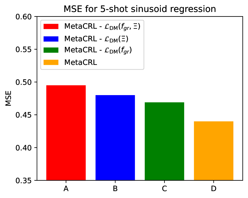
(a) Sinusoid regression

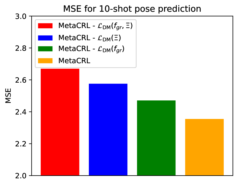
(b) pose prediction

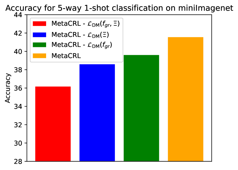
(c) miniImagenet

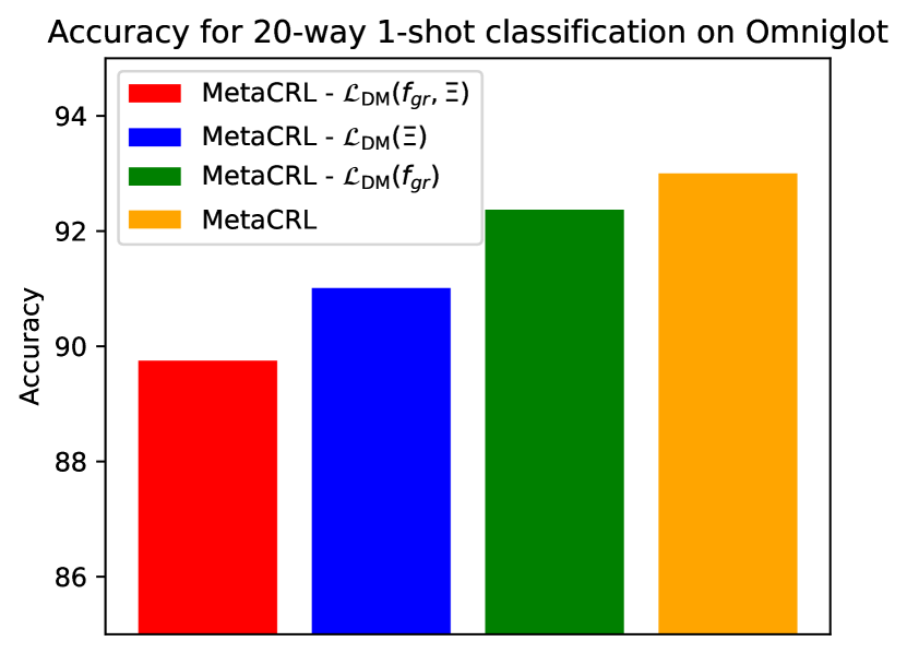
(d) Omniglot

Figure 3: Ablation study of MetaCRL on 4 benchmarks. The backbone in this experiment is MAML.

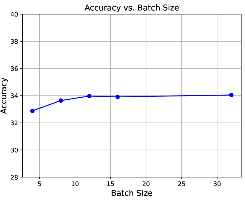
Figure 4: Accuracy (%) of models trained with different batch size on miniImagenet.

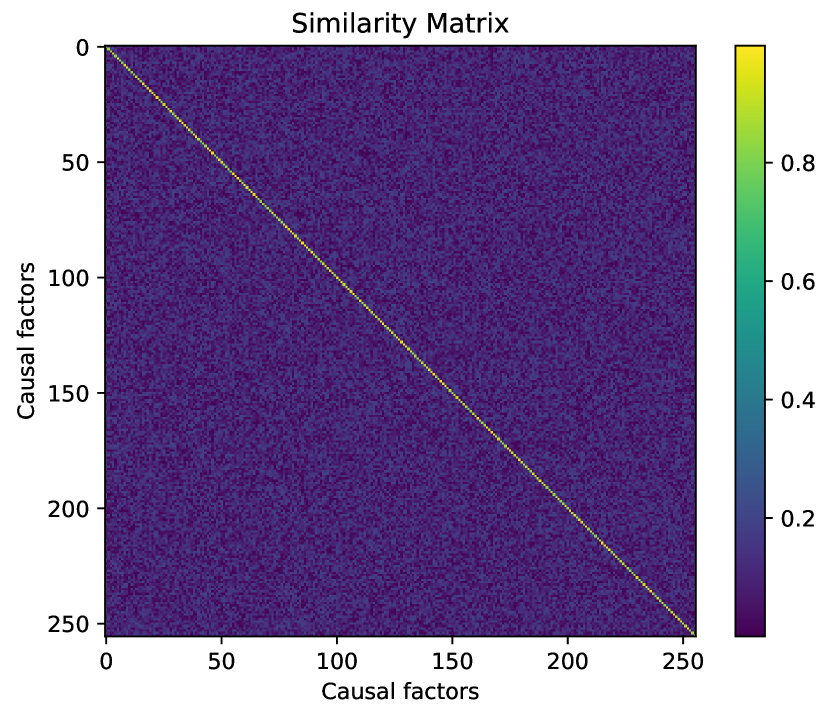
Figure 5: Visualization of the similarity matrix for causal factors in meta-training.

Ablation Study

We conduct ablation study to explore the impact of different regularization terms, that is $\mathcal{L}_{\rm{DM}}(\Xi)$, $\mathcal{L}_{\rm{DM}}(f_{gr})$, and their combination $\mathcal{L}_{\rm{DM}}(f_{gr},\Xi)$. We select two classification and two regression scenarios from the aforementioned experiments for evaluation. The results, as shown in Figure 3, indicate that the first two regularization terms promote the model in all data sets, and the improvement is the largest when combined. Moreover, combining the aforementioned results, despite eliminating the regularization terms, our work still significantly outperforms the backbones, illustrating the effectiveness of the causal mechanism.

Visualization

To better evaluate the effect of MetaCRL, we select MAML as the backbone and visualize the following metrics: (i) accuracy under different batch sizes; and (ii) the similarity between causal factors. The former evaluates MetaCRL’s efficacy in ensuring causality, while the latter assesses the decoupling of causal factors. Figures 5 and 5 show visualizations for these two aspects, respectively. Figure 5 shows that the model’s performance doesn’t decrease as batch size increases, which indicates that MetaCRL effectively eliminates task confounders. Figure 5 demonstrates that the disentangling module successfully decouples causal factors.

Conclusion

In this paper, we propose a novel problem called “Task Confounder” and present a method called MetaCRL to address its unique challenges. We begin by analyzing a counterintuitive performance degradation phenomenon with SCM, revealing spurious correlations between causal factors of the training tasks and the generic label space, called “Task Confounder”. Then, we devise MetaCRL, which consists of two modules: (i) the disentangling module that acquires causal factors; (ii) the causal module that ensures causality of the factors. It is a plug-and-play causal representation learner that can be easily introduced into the meta-learning framework to eliminate task confounders. Extensive experiments demonstrate the effectiveness of our approach. Our work uncovers a novel and significant issue in meta-learning, providing valuable insights for future research.

References

- Arjovsky et al. (2019) Arjovsky, M.; Bottou, L.; Gulrajani, I.; and Lopez-Paz, D. 2019. Invariant Risk Minimization. CoRR, abs/1907.02893.
- Bertinetto et al. (2018) Bertinetto, L.; Henriques, J. F.; Torr, P. H.; and Vedaldi, A. 2018. Meta-learning with differentiable closed-form solvers. arXiv preprint arXiv:1805.08136.
- Chen et al. (2020) Chen, J.; Zhan, L.-M.; Wu, X.-M.; and Chung, F.-l. 2020. Variational metric scaling for metric-based meta-learning. In Proceedings of the AAAI conference on artificial intelligence, volume 34, 3478–3485.
- Du et al. (2020) Du, Y.; Xu, J.; Xiong, H.; Qiu, Q.; Zhen, X.; Snoek, C. G.; and Shao, L. 2020. Learning to learn with variational information bottleneck for domain generalization. In Computer Vision–ECCV 2020: 16th European Conference, Glasgow, UK, August 23–28, 2020, Proceedings, Part X 16, 200–216. Springer.
- Finn, Abbeel, and Levine (2017) Finn, C.; Abbeel, P.; and Levine, S. 2017. Model-agnostic meta-learning for fast adaptation of deep networks. In International conference on machine learning, 1126–1135. PMLR.
- Gordon et al. (2018) Gordon, J.; Bronskill, J.; Bauer, M.; Nowozin, S.; and Turner, R. E. 2018. Meta-learning probabilistic inference for prediction. arXiv preprint arXiv:1805.09921.
- Hospedales et al. (2021) Hospedales, T.; Antoniou, A.; Micaelli, P.; and Storkey, A. 2021. Meta-learning in neural networks: A survey. IEEE transactions on pattern analysis and machine intelligence, 44(9): 5149–5169.
- Hu et al. (2022) Hu, Z.; Zhao, Z.; Yi, X.; Yao, T.; Hong, L.; Sun, Y.; and Chi, E. 2022. Improving multi-task generalization via regularizing spurious correlation. Advances in Neural Information Processing Systems, 35: 11450–11466.
- Islam, Jia, and Bruce (2020) Islam, M. A.; Jia, S.; and Bruce, N. D. 2020. How much position information do convolutional neural networks encode? arXiv preprint arXiv:2001.08248.
- Jamal and Qi (2019) Jamal, M. A.; and Qi, G.-J. 2019. Task agnostic meta-learning for few-shot learning. In Proceedings of the IEEE/CVF Conference on Computer Vision and Pattern Recognition, 11719–11727.
- Jiang et al. (2022) Jiang, Y.; Chen, Z.; Kuang, K.; Yuan, L.; Ye, X.; Wang, Z.; Wu, F.; and Wei, Y. 2022. The Role of Deconfounding in Meta-learning. In International Conference on Machine Learning, 10161–10176. PMLR.
- Koyama and Yamaguchi (2020) Koyama, M.; and Yamaguchi, S. 2020. When is invariance useful in an Out-of-Distribution Generalization problem? arXiv preprint arXiv:2008.01883.
- Lake, Salakhutdinov, and Tenenbaum (2019) Lake, B. M.; Salakhutdinov, R.; and Tenenbaum, J. B. 2019. The Omniglot challenge: a 3-year progress report. Current Opinion in Behavioral Sciences, 29: 97–104.
- Lee et al. (2020) Lee, H. B.; Nam, T.; Yang, E.; and Hwang, S. J. 2020. Meta dropout: Learning to perturb latent features for generalization.
- Lee and Choi (2018) Lee, Y.; and Choi, S. 2018. Gradient-based meta-learning with learned layerwise metric and subspace. In International Conference on Machine Learning, 2927–2936. PMLR.
- Li et al. (2018) Li, D.; Yang, Y.; Song, Y.-Z.; and Hospedales, T. 2018. Learning to generalize: Meta-learning for domain generalization. In Proceedings of the AAAI conference on artificial intelligence, volume 32.
- Li et al. (2017) Li, Z.; Zhou, F.; Chen, F.; and Li, H. 2017. Meta-sgd: Learning to learn quickly for few-shot learning. arXiv preprint arXiv:1707.09835.
- Locatello et al. (2019) Locatello, F.; Bauer, S.; Lucic, M.; Raetsch, G.; Gelly, S.; Schölkopf, B.; and Bachem, O. 2019. Challenging common assumptions in the unsupervised learning of disentangled representations. In international conference on machine learning, 4114–4124. PMLR.
- Mahadevkar et al. (2022) Mahadevkar, S. V.; Khemani, B.; Patil, S.; Kotecha, K.; Vora, D.; Abraham, A.; and Gabralla, L. A. 2022. A review on machine learning styles in computer vision-techniques and future directions. IEEE Access.
- Martin et al. (2019) Martin, E. J.; Polyakov, V. R.; Zhu, X.-W.; Tian, L.; Mukherjee, P.; and Liu, X. 2019. All-assay-Max2 pQSAR: activity predictions as accurate as four-concentration IC50s for 8558 Novartis assays. Journal of chemical information and modeling, 59(10): 4450–4459.
- Mitchell et al. (2021) Mitchell, E.; Rafailov, R.; Peng, X. B.; Levine, S.; and Finn, C. 2021. Offline meta-reinforcement learning with advantage weighting. In International Conference on Machine Learning, 7780–7791. PMLR.
- Nichol and Schulman (2018) Nichol, A.; and Schulman, J. 2018. Reptile: a scalable metalearning algorithm. arXiv preprint arXiv:1803.02999, 2(3): 4.
- Nogueira et al. (2022) Nogueira, A. R.; Pugnana, A.; Ruggieri, S.; Pedreschi, D.; and Gama, J. 2022. Methods and tools for causal discovery and causal inference. Wiley interdisciplinary reviews: data mining and knowledge discovery, 12(2): e1449.
- Oh et al. (2020) Oh, J.; Yoo, H.; Kim, C.; and Yun, S.-Y. 2020. Boil: Towards representation change for few-shot learning. arXiv preprint arXiv:2008.08882.
- Raghu et al. (2019) Raghu, A.; Raghu, M.; Bengio, S.; and Vinyals, O. 2019. Rapid learning or feature reuse? towards understanding the effectiveness of maml. arXiv preprint arXiv:1909.09157.
- Ren et al. (2018) Ren, M.; Triantafillou, E.; Ravi, S.; Snell, J.; Swersky, K.; Tenenbaum, J. B.; Larochelle, H.; and Zemel, R. S. 2018. Meta-learning for semi-supervised few-shot classification. arXiv preprint arXiv:1803.00676.
- Rivolli et al. (2022) Rivolli, A.; Garcia, L. P.; Soares, C.; Vanschoren, J.; and de Carvalho, A. C. 2022. Meta-features for meta-learning. Knowledge-Based Systems, 240: 108101.
- Schrum et al. (2022) Schrum, M. L.; Hedlund-Botti, E.; Moorman, N.; and Gombolay, M. C. 2022. Mind meld: Personalized meta-learning for robot-centric imitation learning. In 2022 17th ACM/IEEE International Conference on Human-Robot Interaction (HRI), 157–165. IEEE.
- Snell, Swersky, and Zemel (2017) Snell, J.; Swersky, K.; and Zemel, R. 2017. Prototypical networks for few-shot learning. Advances in neural information processing systems, 30.
- Song et al. (2022) Song, X.; Zheng, S.; Cao, W.; Yu, J.; and Bian, J. 2022. Efficient and effective multi-task grouping via meta learning on task combinations. Advances in Neural Information Processing Systems, 35: 37647–37659.
- Sung et al. (2018) Sung, F.; Yang, Y.; Zhang, L.; Xiang, T.; Torr, P. H.; and Hospedales, T. M. 2018. Learning to compare: Relation network for few-shot learning. In Proceedings of the IEEE conference on computer vision and pattern recognition, 1199–1208.
- Suter et al. (2019) Suter, R.; Miladinovic, D.; Schölkopf, B.; and Bauer, S. 2019. Robustly disentangled causal mechanisms: Validating deep representations for interventional robustness. In International Conference on Machine Learning, 6056–6065. PMLR.
- Ton, Sejdinovic, and Fukumizu (2021) Ton, J.-F.; Sejdinovic, D.; and Fukumizu, K. 2021. Meta learning for causal direction. In Proceedings of the AAAI Conference on Artificial Intelligence, volume 35, 9897–9905.
- Vinyals et al. (2016) Vinyals, O.; Blundell, C.; Lillicrap, T.; Wierstra, D.; et al. 2016. Matching networks for one shot learning. Advances in neural information processing systems, 29.
- Wang, Zhao, and Li (2021) Wang, H.; Zhao, H.; and Li, B. 2021. Bridging multi-task learning and meta-learning: Towards efficient training and effective adaptation. In International conference on machine learning, 10991–11002. PMLR.
- Xiang, Mottaghi, and Savarese (2014) Xiang, Y.; Mottaghi, R.; and Savarese, S. 2014. Beyond pascal: A benchmark for 3d object detection in the wild. In IEEE winter conference on applications of computer vision, 75–82. IEEE.
- Yang, Zhang, and Cai (2021) Yang, X.; Zhang, H.; and Cai, J. 2021. Deconfounded image captioning: A causal retrospect. IEEE Transactions on Pattern Analysis and Machine Intelligence.
- Yao et al. (2021) Yao, H.; Huang, L.-K.; Zhang, L.; Wei, Y.; Tian, L.; Zou, J.; Huang, J.; et al. 2021. Improving generalization in meta-learning via task augmentation. In International conference on machine learning, 11887–11897. PMLR.
- Yin et al. (2019) Yin, M.; Tucker, G.; Zhou, M.; Levine, S.; and Finn, C. 2019. Meta-learning without memorization. arXiv preprint arXiv:1912.03820.
- Yue et al. (2020) Yue, Z.; Zhang, H.; Sun, Q.; and Hua, X.-S. 2020. Interventional few-shot learning. Advances in neural information processing systems, 33: 2734–2746.
- Zhang et al. (2020) Zhang, D.; Zhang, H.; Tang, J.; Hua, X.-S.; and Sun, Q. 2020. Causal intervention for weakly-supervised semantic segmentation. Advances in Neural Information Processing Systems, 33: 655–666.