FedASMU: Efficient Asynchronous Federated Learning with Dynamic Staleness-aware Model Update

Abstract

As a promising approach to deal with distributed data, Federated Learning (FL) achieves major advancements in recent years. FL enables collaborative model training by exploiting the raw data dispersed in multiple edge devices. However, the data is generally non-independent and identically distributed, i.e., statistical heterogeneity, and the edge devices significantly differ in terms of both computation and communication capacity, i.e., system heterogeneity. The statistical heterogeneity leads to severe accuracy degradation while the system heterogeneity significantly prolongs the training process. In order to address the heterogeneity issue, we propose an Asynchronous Staleness-aware Model Update FL framework, i.e., FedASMU, with two novel methods. First, we propose an asynchronous FL system model with a dynamical model aggregation method between updated local models and the global model on the server for superior accuracy and high efficiency. Then, we propose an adaptive local model adjustment method by aggregating the fresh global model with local models on devices to further improve the accuracy. Extensive experimentation with 6 models and 5 public datasets demonstrates that FedASMU significantly outperforms baseline approaches in terms of accuracy (0.60% to 23.90% higher) and efficiency (3.54% to 97.98% faster).

10cm(5.5cm,18cm) To appear in AAAI 2024

1 Introduction

In recent years, numerous edge devices have been generating large amounts of distributed data.Due to the implementation of laws and regulations, e.g., General Data Protection Regulation (GDPR) (EU 2018), the traditional training approach, which aggregates the distributed data into a central server or a data center, becomes almost impossible. As a promising approach, Federated Learning (FL) (Kairouz et al. 2021; Liu et al. 2022a) enables collaborative model training by transferring gradients or models instead of raw data. FL avoids privacy or security issues incurred by direct raw data transfer while exploiting multiple edge devices to train a global model. FL has been applied in diverse areas, such as computer vision (Liu et al. 2020), nature language processing (Liu et al. 2021), bioinformatics (Chen et al. 2021), and healthcare (Nguyen et al. 2022a).

Traditional FL typically exploits a parameter server (server) (Li et al. 2014; Liu et al. 2023a) to coordinate the training process on each device with a synchronous (McMahan et al. 2017; Li et al. 2020; Liu et al. 2023b; Jia et al. 2023) mechanism. The synchronous training process generally consists of multiple rounds and each round contains five steps. First, the server selects a set of devices (Shi et al. 2020). Second, the server broadcasts the global model to the selected devices. Third, local training is carried out with the data in each selected device. Fourth, each device uploads the updated model (gradients) to the server. Fifth, the server aggregates the uploaded models to generate a new global model when all the selected devices complete the aforementioned four steps. Although the synchronous mechanism is effective and simple to implement, stragglers may significantly prolong the training process (Jiang et al. 2022) with heterogeneous devices (Lai et al. 2021; Yang et al. 2021). Powerful devices may remain idle when the server is waiting for stragglers (Wu et al. 2020), incurring significant efficiency degradation.

Within the FL paradigm, the devices are typically highly heterogeneous in terms of computation and communication capacity (Li, Ota, and Dong 2018; Wu et al. 2020; Nishio and Yonetani 2019; Che et al. 2022, 2023b) and data distribution (McMahan et al. 2017; Li et al. 2020; Wang et al. 2020; Che et al. 2023a). Some devices may complete the local training and update the model within a short time, while some other devices may take a much longer time to finish this process and may fail to upload the model because of modest bandwidth or high latency, which is denoted by system heterogeneity. In addition, the data in each device may be non-Independent and Identically Distributed (non-IID) data, which refers to statistical heterogeneity. The statistical heterogeneity can lead to diverse local objectives (Wang et al. 2020) and client drift (Karimireddy et al. 2020; Hsu, Qi, and Brown 2019) issues, which degrades the accuracy of the global model in FL.

Asynchronous FL (Xu et al. 2021; Wu et al. 2020; Nguyen et al. 2022a) enables the server to aggregate the uploaded models without waiting for stragglers, which improves the efficiency. However, this mechanism may encounter low accuracy brought by stale uploaded models and non-IID data (Zhou et al. 2021a). For instance, when a device uploads a model updated based on an old global model, the global model has already been updated multiple times. Then, the simple aggregation of the uploaded model may drag the global model to previous status, which corresponds to inferior accuracy. In addition, the asynchronous FL mechanism may fail to converge (Su and Li 2022) due to the lack of the staleness control (Xie, Koyejo, and Gupta 2019).

Existing works address the system heterogeneity and the statistical heterogeneity separately. Some works focus on device scheduling (Shi et al. 2020; Shi, Zhou, and Niu 2020; Wu et al. 2020; Zhou et al. 2022; Liu et al. 2022b) to avoid the inefficiency incurred by stragglers while this mechanism may correspond to inferior accuracy due to insufficient participation of devices. Asynchronous FL approaches are proposed to mitigate the system heterogeneity while they either exploit static polynomial formula to deal with the staleness (Xie, Koyejo, and Gupta 2019; Su and Li 2022; Chen, Mao, and Ma 2021) or leverage simple attention mechanism (Chen et al. 2020). However, they cannot dynamically adjust the importance of each uploaded model within the model aggregation process, which leads to modest accuracy. Some other approaches introduce regularization (Li et al. 2020), gradient normalization (Wang et al. 2020), and momentum methods (Hsu, Qi, and Brown 2019; Jin et al. 2022) to address the statistical heterogeneity, while they focus on synchronous FL.

In this paper, we propose an original Asynchronous Federated learning framework with Staleness-aware Model Update (FedASMU). To address the system heterogeneity, we design an asynchronous FL system and propose a dynamical adjustment method to update the importance of updated local models and the global model based on both the staleness and the local loss for superior accuracy and high efficiency. We enable devices to adaptively aggregate fresh global models so as to reduce the staleness of the local model. We summarize the major contributions in this paper as follows:

• We propose a novel asynchronous FL system model with a dynamic model aggregation method on the server, which adjusts the importance of updated local models and the global model based on the staleness and the impact of local loss for superior accuracy and high efficiency.

• We propose an adaptive local model adjustment method on devices to integrate fresh global models into the local model so as to reduce staleness for superb accuracy. The model adjustment consists of a Reinforcement Learning (RL) method to select a proper time slot to retrieve global models and a dynamic method to adjust the local model aggregation.

• We conduct extensive experiments with 9 state-of-the-art baseline approaches, 6 typical models, and 5 public real-life datasets, which reveals FedASMU can well address the heterogeneity issues and significantly outperforms the baseline approaches.

The rest of the paper is organized as follows. We present the related work in Section 2. Then, we formulate the problem and explain the system model in Section 3. We propose the staleness-aware model update in Section 4. The experimental results are given in Section 5. Finally, Section 6 concludes the paper.

2 Related Work

A bunch of FL approaches (McMahan et al. 2017; Li et al. 2020; Wang et al. 2020; Karimireddy et al. 2020; Acar et al. 2021) have been designed to collaboratively train a global model utilizing the distributed data in mobile devices. Most of them (Bonawitz et al. 2019) exploit a synchronous mechanism to perform the model aggregation on the server. With the synchronous mechanism, the server needs to wait for all the selected devices to upload models before the model aggregation, which is inefficient because of stragglers. Due to diverse device availability and system heterogeneity, the probability of the occurrence of the straggler effect increases when the scale of devices becomes large (Li et al. 2014).

Three types of approaches are proposed to address the system heterogeneity with the synchronous mechanism. The first type is to schedule proper devices to perform the local training process (Shi et al. 2020; Shi, Zhou, and Niu 2020; Wu et al. 2020) while considering the computation and communication capacity to achieve load balance among multiple devices. However, this approach may significantly reduce the participation frequency of some modest devices, which degrades accuracy. Second, pruning (Zhang et al. 2022) or dropout (Horvath et al. 2021) techniques are leveraged during the training process, while incurring lossy compression and modest accuracy. Third, the device clustering approach (Li et al. 2022) groups the devices of similar capacity into the same cluster, and utilizes a hierarchical architecture (Abad et al. 2020) to perform model aggregation. All these approaches focus on the synchronous mechanism with low efficiency and may incur severe accuracy degradation due to statistical heterogeneity.

Multiple model aggregation methods (Karimireddy et al. 2020; Mitra et al. 2021; Sattler, Müller, and Samek 2020) exist to handle the statistical heterogeneity with the synchronous mechanism. In particular, regularization (Li et al. 2020; Acar et al. 2021), gradient normalization (Wang et al. 2020), classifier calibration (Luo et al. 2021), and momentum-based (Hsu, Qi, and Brown 2019; Reddi et al. 2021) methods adjust the local objectives to reduce the accuracy degradation brought by heterogeneous data. Contrastive learning (Li, He, and Song 2021), personalization (Sun et al. 2021; Ozkara et al. 2021), meta-learning-based method (Khodak, Balcan, and Talwalkar 2019), and multi-task learning (Smith et al. 2017) adapt the global model or local models to non-IID data. However, these methods cannot dynamically adjust the importance of diverse models and only focus on the synchronous mechanism.

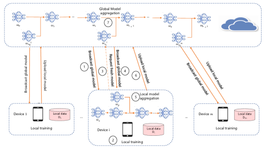
Figure 1: The system model of FedASMU.

To conquer the system heterogeneity problem, asynchronous FL (Xu et al. 2021; Nguyen et al. 2022a) enables the global model aggregation without waiting for all the devices. The asynchronous FL can be performed once a model is uploaded from an arbitrary device (Xie, Koyejo, and Gupta 2019) or when multiple models are buffered (Nguyen et al. 2022b). However, the old uploaded models may drag the global model to a previous status, which significantly degrades the accuracy (Su and Li 2022). Several methods are proposed to improve the accuracy of asynchronous FL. For instance, the impact of the staleness and the divergence of model updates is considered to adjust the importance of uploaded models (Su and Li 2022), which cannot dynamically adapt the weights based on the training status, e.g., loss values. The attention mechanism and the average local training time are exploited to adjust the weights of uploaded models (Chen et al. 2020) without the consideration of staleness. In addition, the uploaded model with severe staleness can be replaced by the latest global model (Wu et al. 2020) to reduce the impact of staleness while losing important information from the device. Furthermore, a staleness-based polynomial formula can be utilized to assign high weights to fresh models (Park et al. 2021; Xie, Koyejo, and Gupta 2019; Chen, Mao, and Ma 2021) while the loss value of the model can be leveraged to adjust the importance of models (Park et al. 2021). However, these methods only consider static formulas, which cannot dynamically adjust the importance of models for the objective of minimizing the loss so as to improve the accuracy.

Different from the existing works, we propose an asynchronous FL framework, i.e., FedASMU, to address the system heterogeneity. FedASMU adjusts the importance of uploaded models based on the staleness while enabling devices to adaptively aggregate fresh global models to further mitigate the staleness issues, which handles the statistical heterogeneity.

3 Aysnchronous System Architecture

In this section, we present the problem formulation for FL and the asynchronous system model.

We consider an FL setting composed of a powerful server and $m$ devices, denoted by $\mathcal{M}$, which collaboratively train a global model (the main notations are summarized in Appendix). Each device $i$ stores a local dataset $\mathcal{D}_{i}=\{\boldsymbol{x}_{i,d}\in\mathbb{R}^{s},y_{i,d}\in\mathbb{R}\}_{d=1}^{D_{i}}$ with $D_{i}=|\mathcal{D}_{i}|$ data samples where $\boldsymbol{x}_{i,d}$ is the $d$-th $s$-dimensional input data vector, and $y_{i,d}$ is the label of $\boldsymbol{x}_{i,d}$. The whole dataset is denoted by $\mathcal{D}=\bigcup_{i\in\mathcal{M}}\mathcal{D}_{i}$ with $D=\sum_{i\in\mathcal{M}}D_{i}$. Then, the objective of the training process within FL is:

$$\vspace{-3mm}\min_{\boldsymbol{w}}\Big{\{}\mathcal{F}(\boldsymbol{w})\triangleq\frac{1}{|D|}\sum_{i\in\mathcal{M}}|\mathcal{D}_{i}|\mathcal{F}_{i}(\boldsymbol{w})\Big{\}}, \mathcal{P}$$ ()

where $\boldsymbol{w}$ represents the global model, $\mathcal{F}_{i}(\boldsymbol{w})$ is the local loss function defined as $\mathcal{F}_{i}(\boldsymbol{w})\triangleq\frac{1}{|D_{i}|}\sum_{\{\boldsymbol{x}_{i,d},y_{i,d}\}\in\mathcal{D}_{i}}F(\boldsymbol{w},\boldsymbol{x}_{i,d},y_{i,d})$, and $F(\boldsymbol{w},\boldsymbol{x}_{i,d},y_{i,d})$ is the loss function to measure the error of the model parameter $\boldsymbol{w}$ on data sample $\{\boldsymbol{x}_{i,d},y_{i,d}\}$.

In order to address the problem defined in Formula $\mathcal{P}$, we propose an asynchronous FL framework as shown in Figure 1. The server triggers the local training of $m^{\prime}$ devices with a constant time period $\mathcal{T}$. The training process is composed of multiple global rounds. At the beginning of the training, the version of the global model is 0. Then, after each global round, the version of the global model increases by 1. Each global round is composed of 7 steps. First, the server triggers $m^{\prime}(m^{\prime}\leq m)$ devices and broadcasts the global model $\boldsymbol{w}_{o}$ to each device at Step ①. The $m^{\prime}$ devices are randomly selected available devices. Then, each device performs local training with its local dataset at Step ②. During the local training process, Device $i$ requests a fresh global model (Step ③) from the server to reduce the staleness of the local training as the global model may be updated at the same time. Then, the server sends the global model $\boldsymbol{w}_{g}$ to the device at Step ④, if $\boldsymbol{w}_{g}$ is newer than $\boldsymbol{w}_{o}$, i.e., $g>o$. After receiving the fresh global model, the device aggregates the global model and the latest local model to a new model at Step ⑤ and continues the local training with the new model. When the local training is completed, Device $i$ uploads the local model to the server at Step ⑥. Finally, the server aggregates the latest global model $\boldsymbol{w}_{t}$ with the uploaded model $\boldsymbol{w}^{i}_{o}$ at Step ⑦. When aggregating the global model $\boldsymbol{w}_{t}$ and the uploaded local model $\boldsymbol{w}^{i}_{o}$, the staleness of the local model is calculated as $\tau_{i}=t-o+1$. When the staleness $\tau_{i}$ is significant, the local model may drag the global model to a previous version corresponding to inferior accuracy due to legacy information. We discard the uploaded local models when the staleness exceeds a predefined threshold $\tau$ to meet the staleness bound so as to ensure the convergence (Ho et al. 2013).

4 Staleness-aware Model Update

In this section, we propose our dynamic staleness-aware model aggregation method on the server (Step ⑦) and the adaptive local model adjustment method on devices (Steps ③ and ⑤).

Dynamic Model Update on the Server

In this subsection, we propose our dynamic staleness-aware model update method on the server. When the server receives an uploaded model $\boldsymbol{w}_{o}^{i}$ from Device $i$ with the original version $o$, it updates the current global model $\boldsymbol{w}_{t}$ according to the following formula:

$$\boldsymbol{w}_{t+1}=(1-\alpha^{i}_{t})\boldsymbol{w}_{t}+\alpha^{i}_{t}\boldsymbol{w}_{o}^{i},\vspace{-1mm}$$ (1)

where $\alpha^{i}_{t}$ represents the importance of the uploaded model from Device $i$ at global round $t$, which may have a significant impact on the accuracy of the aggregated model (Xie, Koyejo, and Gupta 2019). Then, we decompose the problem defined in Formula $\mathcal{P}$ to the following bi-level optimization problem (Bard 1998):

$$\min_{\boldsymbol{w},\boldsymbol{A}}\Big{\{} \mathcal{F}(\boldsymbol{w},\boldsymbol{A})\triangleq\frac{1}{|D|}\sum_{i\in\mathcal{M}}|\mathcal{D}_{i}|\mathcal{F}_{i}(\boldsymbol{w}(\boldsymbol{A}))\Big{\}},$$

$$\boldsymbol{w}(\boldsymbol{A})=(1-\alpha^{i}_{t})\boldsymbol{w}_{t}+\alpha^{i}_{t}\boldsymbol{w}_{o}^{i},\alpha^{i}_{t}\in\boldsymbol{A}, \mathcal{P}1$$ ()

s.t. $$~{}\boldsymbol{w}^{i}_{o}=\mathop{\rm argmin}_{\boldsymbol{w}^{i}_{o}}\mathcal{F}_{i}(\boldsymbol{w}^{i}_{o})~{}\forall~{}i\in\mathcal{M}, \mathcal{P}2$$ ()

$$~{}\boldsymbol{A}=\mathop{\rm argmin}_{\boldsymbol{A}}\mathcal{F}(\boldsymbol{w},\boldsymbol{A}),\vspace{-4mm} \mathcal{P}3$$ ()

where $\boldsymbol{A}=\{\alpha_{t}^{1},\alpha_{t}^{2},...,\alpha_{t}^{m}\}$ is a set of values corresponding to the importance of the uploaded models from devices. Problem $\mathcal{P}2$ is the minimization of the local loss function, which is detailed in Section 4. Inspired by (Xie, Koyejo, and Gupta 2019), we propose a dynamic polynomial function to represent $\alpha^{i}_{t}$ defined in Formula 4 for Problem $\mathcal{P}3$.

$$\xi^{i}_{t}(o) =\frac{\lambda^{i}_{t}}{\sqrt{t}(t-o+1)^{\sigma^{i}_{t}}}+\iota^{i}_{t},$$

$$\alpha^{i}_{t}(o) =\frac{\mu_{\alpha}\xi^{i}_{t}(o)}{1+\mu_{\alpha}\xi^{i}_{t}(o)},\vspace{-4mm}$$ (2)

where $\mu_{\alpha}$ refers to a hyper-parameter, $t-o+1$ represents the staleness, $t$ represents the version of the current global model, $o$ corresponds to the version of the global model that Device $i$ received before local training, $\lambda^{i}_{t}$, $\sigma^{i}_{t}$, and $\iota^{i}_{t}$ are control parameters on Device $i$ at the $t$-th global round. These three parameters are dynamically adjusted according to Formula 4 to reduce the loss of the global model (see details in Appendix).

$$\lambda^{i}_{t} =\lambda^{i}_{o-1}-\eta_{\lambda^{i}}\nabla_{\lambda^{i}_{o-1}}\mathcal{F}(\boldsymbol{w}_{o}),$$

$$\sigma^{i}_{t} =\sigma^{i}_{o-1}-\eta_{\sigma^{i}}\nabla_{\sigma^{i}_{o-1}}\mathcal{F}(\boldsymbol{w}_{o}),$$ (3)

$$\iota^{i}_{t} =\iota^{i}_{o-1}-\eta_{\iota^{i}}\nabla_{\iota^{i}_{o-1}}\mathcal{F}(\boldsymbol{w}_{o}),$$

where $\eta_{\lambda^{i}}$, $\eta_{\sigma^{i}}$, and $\eta_{\iota^{i}}$ represent the corresponding learning rates for dynamic adjustment, $\nabla_{\lambda^{i}_{o-1}}\mathcal{F}(\boldsymbol{w}_{o})$, $\nabla_{\sigma^{i}_{o-1}}\mathcal{F}(\boldsymbol{w}_{o})$, and $\nabla_{\iota^{i}_{o-1}}\mathcal{F}(\boldsymbol{w}_{o})$ correspond to the respective partial derivatives of the loss function.

Algorithm 1 FedASMU on the Server

0:   $T$: The maximum number of global rounds $m^{\prime}$: The number of devices to be triggered $\tau$: The predefined staleness limit $\mathcal{T}$: The constant time period to trigger devices $\boldsymbol{w}_{0}$: The initial global model $\lambda_{0}$, $\sigma_{0}$, $\iota_{0}$: The initial control parameters$\eta_{\lambda^{i}}$, $\eta_{\sigma^{i}}$, $\eta_{\iota^{i}}$: The learning rates for the dynamic adjustment

0:   $\boldsymbol{w}_{T}$: The global model at Round $T$

1:  while The training is not finished (in parallel) do

2:     if Should trigger new devices then

3:        Trigger and broadcast the global model to $m^{\prime}$ devices for parallel local training

4:        Sleep $\mathcal{T}$

5:     end if

6:  end while

7:  for $t$ in $\{1,2,...,T\}$ do

8:     Receive $\boldsymbol{w}^{i}_{o}$

9:     if $t-o+1>\tau$ then

10:        Discard $\boldsymbol{w}^{i}_{o}$ and continue

11:     else

12:        Update $\lambda_{t}^{i}$, $\sigma_{t}^{i}$, $\iota_{t}^{i}$ according to Formula 4

13:        Update $\alpha^{i}_{t}$ utilizing Formula 4

14:        Update $\boldsymbol{w}_{t}$ exploiting Formula 1

15:     end if

16:  end for

The model aggregation algorithm of FedASMU on the server is shown in Algorithm 1. A separated thread periodically triggers $m^{\prime}$ devices when the number of devices performing training is smaller than a predefined value (Lines 1 - 6). When the server receives $\boldsymbol{w}^{i}_{o}$ (Line 8), it verifies if the uploaded model is within the staleness bound (Line 9). If not, the server ignores the $\boldsymbol{w}^{i}_{o}$ (Line 10). Otherwise, the server updates the control parameters $\lambda_{t}^{i}$, $\sigma_{t}^{i}$, $\iota_{t}^{i}$ according to Formula 4 (Line 12) and calculates $\alpha^{i}_{t}$ based on Formula 4 (Line 13). Afterward, the server updates the global model (Line 14). Please see the details of the convergence analysis in Appendix.

Adaptive Model Update on Devices

In this subsection, we present the local training process with an adaptive local model adjustment method on devices to address Problem $\mathcal{P}2$.

When Device $i$ is triggered to perform local training, it receives a global model $\boldsymbol{w}_{o}$ from the server and takes it as the initial local model $\boldsymbol{w}_{o,0}$. Within the local training process, the Stochastic Gradient Descent (SGD) approach (Robbins and Monro 1951; Zinkevich et al. 2010) is exploited to update the local model based on the local dataset $\mathcal{D}_{i}$ as defined in Formula 4.

$$\boldsymbol{w}_{o,l}=\boldsymbol{w}_{o,l-1}-\eta_{i}\nabla\mathcal{F}_{i}(\boldsymbol{w}_{o,l-1},\zeta_{l-1}),\zeta_{l-1}\sim\mathcal{D}_{i},$$ (4)

where $o$ is the version of the global model, $l$ represents the number of local epochs, $\eta_{i}$ refers to the learning rate on Device $i$, and $\nabla\mathcal{F}_{i}(\cdot)$ corresponds to the gradient based on an unbiased sampled mini-batch $\zeta_{l-1}$ from $\mathcal{D}_{i}$.

In order to reduce the gap between the local model and the global model, we propose aggregating the fresh global model with the local model during the local training process of the devices. During the local training, the global model may be intensively updated simultaneously. Thus, the model aggregation with the fresh global model can well reduce the gap between the local model and the global model. However, it is complicated to determine the time slot to send the request and the weights to aggregate the fresh global model. In this section, we first propose a Reinforcement Learning (RL) method to select a proper time slot. Then, we explain the dynamic local model aggregation method.

Intelligent Time Slot Selection

We propose an RL-based intelligent time slot selector to choose a proper time slot to request a fresh global model from the server. In order to reduce communication overhead, we assume only one fresh global model is received during the local training. When the request is sent early, the server performs few updates and the final updated local model may still suffer from severe staleness. However, when the request is sent late, the local update cannot leverage the information from the fresh global model, corresponding to inferior accuracy. Thus, it is beneficial to choose a proper time slot to send the request.

The intelligent time slot selector is composed of a meta model on the server and a local model on each device. The meta model generates an initial time slot decision for each device, and is updated when a device performs the first local training. The local model is initialized with the initial time slot and updated within the device during the following local training to generate personalized proper time slot for the fresh global model request. We exploit a Long Short-Term Memory (LSTM)-based network with a fully connected layer for the meta model and a $\mathcal{Q}$-learning method (Watkins and Dayan 1992) for each local model. Both the meta model and the local model generate the probability for each time slot. We exploit the $\epsilon$-greedy strategy (Xia and Zhao 2015) to perform the selection.

Algorithm 2 FedASMU on Devices

0:   $t$: The number of the meta model update $t_{i}$: The number of local model aggregation $\mathcal{L}^{i}$: The maximum number of epochs on Device $i$ $\boldsymbol{w}_{o}$: The original global model with Version $o$ $\boldsymbol{w}_{g}$: The fresh global model with Version $g$$\theta^{i}_{t-1}$: The parameters of the meta model $\gamma^{i}_{t_{i}-1}$, $\upsilon^{i}_{t_{i}-1}$: The control parameters

0:   $\boldsymbol{w}^{i}_{o,\mathcal{L}}$: The trained local model

1:  $l^{*}\leftarrow$ Generate a time slot using $\theta^{i}_{t-1}$ or $\mathcal{H}_{t_{i}-1}^{i}$

2:  $\boldsymbol{w}^{i}_{o,0}\leftarrow\boldsymbol{w}_{o}$

3:  for $l$ in $\{1,2,...,\mathcal{L}^{i}\}$ do

4:     if $l=l^{*}$ then

5:        Send a fresh global model request to server

6:        Receive $\boldsymbol{w}_{g}$

7:     end if

8:     if $\boldsymbol{w}_{g}$ is updated then

9:        $\beta^{i}_{t_{i}-1}\leftarrow$ Calculation based on Formula 4

10:        Update $\boldsymbol{w}_{o,l-1}$ with $\beta^{i}_{t_{i}-1}$, $\boldsymbol{w}_{g}$ and Formula 7

11:        Update $\gamma^{i}_{t_{i}}$ and $\upsilon^{i}_{t_{i}}$ based on Formula 4

12:        $\mathcal{R}\leftarrow loss_{o,l}^{b,i}-loss_{o,l}^{a,i}$

13:        $b_{t_{i}}\leftarrow(1-\rho)b_{t_{i}-1}+\rho\mathcal{R}$

14:        Update $\theta_{t}$ or $\mathcal{H}_{t_{i}}^{i}$ with $\mathcal{R}$

15:     end if

16:     Update $\boldsymbol{w}_{o,l}$ based on Formula 4

17:  end for

Table 1: The accuracy and training time with FedASMU and diverse baseline approaches. “Acc” represents the convergence accuracy of the global model. “Time” refers to the training time to achieve a target accuracy, i.e., 0.30 for LeNet with CIFAR-10, 0.13 for LeNet with CIFAR-100, 0.40 for CNN with CIFAR-10, 0.15 for CNN with CIFAR-100, 0.25 for ResNet with CIFAR-100, and 0.12 for ResNet with Tiny-ImageNet. “/” represents that the method does not achieve the target accuracy.

Method	LeNet				CNN				ResNet
	CIFAR-10		CIFAR-100		CIFAR-10		CIFAR-100		CIFAR-100		Tiny-ImageNet
	Acc	Time	Acc	Time	Acc	Time	Acc	Time	Acc	Time	Acc	Time
FedASMU	0.486	8800	0.182	20737	0.603	10109	0.277	30569	0.358	16027	0.171	22415
FedAvg	0.431	125514	0.168	95306	0.551	117794	0.243	73145	0.299	109680	0.146	155023
FedProx	0.363	126958	0.172	93430	0.371	/	0.243	73145	0.302	109680	0.148	151935
MOON	0.302	437531	0.172	93430	0.47	100302	0.212	252703	0.302	106021	0.149	139444
FedDyn	0.279	/	0.147	70260	0.507	43974	0.193	52874	0.328	73711	0.142	103661
FedAsync	0.478	36565	0.158	102113	0.491	24931	0.23	37160	0.315	21107	0.143	31288
PORT	0.305	366182	0.104	/	0.385	/	0.145	/	0.314	35712	0.134	78155
ASO-Fed	0.408	83712	0.153	110942	0.482	92246	0.208	103090	0.276	198797	0.122	359899
FedBuff	0.365	9829	0.174	25791	0.364	/	0.201	65736	0.315	27672	0.148	43523
FedSA	0.306	21077	0.0835	/	0.508	20415	0.189	94169	0.195	/	0.116	/

Within the local training process, we define the reward as the difference between the loss value before model aggregation and that after aggregation. For instance, before aggregating the fresh global model with the request sent after $l^{*}$ local epochs, the loss value of $\mathcal{F}_{i}(\boldsymbol{w}_{o,l^{*}},\zeta_{l^{*}})$ is $loss_{o,l^{*}}^{b,i}$ and that after aggregation is $loss_{o,l^{*}}^{a,i}$. Then, the reward is $\mathcal{R}=loss_{o,l^{*}}^{b,i}-loss_{o,l^{*}}^{a,i}$. Inspired by (Zoph and Le 2017), we update the LSTM model with Formula 5 once an initial aggregation is performed.

$$\theta_{t}=\theta_{t-1}+\eta_{RL}\sum_{l=1}^{\mathcal{L}}\nabla_{\theta_{t-1}}\log P(\mathcal{s}_{l}|\mathcal{s}_{(l-1):1};\theta_{t-1})(\mathcal{R}-b_{t}),$$ (5)

where $\theta_{t}$ represents the parameters in the meta model after the $t$-th meta model update, $\eta_{RL}$ refers to the learning rate for the training process of RL, $\mathcal{L}$ is the maximum number of local epochs, $\mathcal{s}_{l}$ corresponds to the decision of sending the request (1) or not (0) after the $l$-th local epoch, and $b_{t}$ is a base value to reduce the bias of the model. The model is pre-trained with some historical data and dynamically updated during the training process of FedASMU on each device. The $\mathcal{Q}$-learning method manages a mapping $\mathcal{H}^{i}$ between the decision and the reward on Device $i$, which is updated with a weighted average of historical values and reward as shown in Formula 4, inspired by (Dietterich 2000).

$$\mathcal{H}^{i}_{t_{i}}(l^{*}_{t_{i}-1},a_{t_{i}-1})=\mathcal{H}^{i}_{t_{i}-1}(l^{*}_{t_{i}-1},a_{t_{i}-1})+\phi(\mathcal{R}$$

$$+\psi\max_{a}{\mathcal{H}^{i}_{t_{i}-1}(l^{*}_{t_{1}},a)-\mathcal{H}^{i}_{t_{i}-1}(l^{*}_{t_{i}-1},a_{t_{i}-1})}),\vspace{-8mm}$$ (6)

where $a_{t_{i}-1}$ represents the action, $l^{*}_{t_{i}-1}$ represents the number of local epochs to send the request within the $(t_{i}-1)$-th local model aggregation, $\phi$ and $\psi$ are hyper-parameters. The action is within an action space, i.e., $a_{t_{i}-1}\in\{add,stay,minus\}$, with $add$ representing adding 1 epoch to $l^{*}_{t_{i}-1}$ ($l^{*}_{t_{i}}=l^{*}_{t_{i}-1}+1$), $stay$ representing staying with the same epoch ($l^{*}_{t_{i}}=l^{*}_{t_{i}-1}+1$), and $minus$ representing removing 1 epoch from $l^{*}_{t_{i}-1}$ ($l^{*}_{t_{i}}=l^{*}_{t_{i}-1}-1$).

Dynamic Local Model Aggregation

When receiving a fresh global model $\boldsymbol{w}_{g}$, Device $i$ performs local model aggregation with its current local model $\boldsymbol{w}_{o,l}^{b}$ utilizing Formula 7.

$$\boldsymbol{w}_{o,l}^{a}=(1-\beta^{i}_{t_{i}-1})\boldsymbol{w}_{o,l}^{b}+\beta^{i}_{t_{i}-1}\boldsymbol{w}_{g},\vspace{-1mm}$$ (7)

where $\beta^{i}_{t_{i}-1}$ is the weight of the fresh global model on Device $i$ at the $(t_{i}-1)$-th local global model aggregation. Formula 7 differs from Formula 1 as the received fresh global model corresponds to a higher global version. We exploit Formula 4 to calculate $\beta^{i}_{t-1}$.

$$\phi^{i}_{t_{i}-1}(g,o) =\frac{\gamma^{i}_{t_{i}-1}}{\sqrt{g}}(1-\frac{\upsilon^{i}_{t_{i}-1}}{\sqrt{g-o+1}}),$$

$$\beta^{i}_{t_{i}-1}(g,o) =\frac{\mu_{\beta}\phi^{i}_{t_{i}-1}(g,o)}{1+\mu_{\beta}\phi^{i}_{t_{i}-1}(g,o)},\vspace{-4mm}$$ (8)

where $\mu_{\beta}$ is a hyper-parameter, $\gamma^{i}_{t_{i}-1}$ and $\upsilon^{i}_{t_{i}-1}$ are control parameters to be dynamically adjusted based on Formula 4 (see details in Appendix).

$$\gamma^{i}_{t_{i}} =\gamma^{i}_{t_{i}-1}-\eta_{\gamma^{i}}\nabla_{\gamma^{i}_{t_{i}-1}}\mathcal{F}_{i}(\boldsymbol{w}_{o,l}^{b},\zeta_{l-1}),$$

$$\upsilon^{i}_{t_{i}} =\upsilon^{i}_{t_{i}-1}-\eta_{\upsilon^{i}}\nabla_{\upsilon^{i}_{t_{i}-1}}\mathcal{F}_{i}(\boldsymbol{w}_{o,l}^{b},\zeta_{l-1}),\zeta_{l-1}\sim\mathcal{D}_{i},\vspace{-4mm}$$ (9)

where $\eta_{\gamma^{i}}$ and $\eta_{\upsilon^{i}}$ are learning rates for $\gamma^{i}_{t_{i}}$ and $\upsilon^{i}_{t_{i}}$.

The model update algorithm of FedASMU on devices is shown in Algorithm 2. First, an epoch number $l^{*}$ (time slot) to send a request for a fresh global model is generated based on $\theta_{t-1}$ when $t=1$ or $\mathcal{H}_{t_{i}-1}^{i}$ when $t\neq 1$ (Line 1). In the $l^{*}$-th local epoch, the device sends a request to the server (Line 5), and it waits for the fresh global model (Line 6). After receiving the fresh global model (Line 8), we exploit Formula 4 to update $\beta^{i}_{t_{i}-1}$ (Line 9), Formula 7 to update $\boldsymbol{w}_{o,l-1}$ (Line 10), Formula 4 to update $\gamma^{i}_{t-1}$ and $\upsilon^{i}_{t-1}$ (Line 11), the reward values (Line 12), $b_{t-1}$ with $\rho$ being a hyper-parameter (Line 13), $\theta_{t}$ when $t=1$ or $\mathcal{H}_{t_{i}-1}^{i}$ when $t\neq 1$ (Line 14). Finally, the local model is updated (Line 16).

5 Experiments

In this section, we present the experimental comparison of FedASMU with 9 state-of-the-art approaches. We first present the experimentation setup. Then, we demonstrate the experimental results.

Experimental Setup

We consider an FL environment with a server and 100 heterogeneous devices. We consider both the asynchronous baseline approaches, i.e., FedAsync (Xie, Koyejo, and Gupta 2019), PORT (Su and Li 2022), ASO-Fed (Chen et al. 2020), FedBuff (Nguyen et al. 2022b), FedSA (Chen, Mao, and Ma 2021), and synchronous baseline approaches, i.e., FedAvg (McMahan et al. 2017), FedProx (Li et al. 2020), MOON (Li, He, and Song 2021), and FedDyn (Acar et al. 2021). We utilize 5 public datasets, i.e., Fashion-MNIST (FMNSIT) (Xiao, Rasul, and Vollgraf 2017), CIFAR-10 and CIFAR-100 (Krizhevsky, Hinton et al. 2009), IMDb (Zhou et al. 2021b), and Tiny-ImageNet (Le and Yang 2015). The data on each device is non-IID based on a Dirichlet distribution (Li et al. 2021). We leverage 6 models to deal with the data, i.e., LeNet5 (LeNet) (LeCun et al. 1989), a synthetic CNN network (CNN), ResNet20 (ResNet) (He et al. 2016), AlexNet (Krizhevsky, Sutskever, and Hinton 2012), TextCNN (Zhou et al. 2021b), and VGG-11 (VGG) (Simonyan and Zisserman 2015). Please see details in Appendix.

Evaluation of FedASMU

Table 2: The accuracy and training time with FedASMU and diverse baseline approaches. “Acc” is the convergence accuracy of the global model. “Time” refers to the training time to achieve a target accuracy, i.e., 0.40 for AlexNet with CIFAR-10, 0.12 for AlexNet with CIFAR-100, 0.45 for VGG with CIFAR-10, 0.12 for VGG with CIFAR-100, 0.85 for TextCNN, and 0.70 for LeNet. “/” represents that the method does not achieve the target accuracy.

Method	AlexNet				VGG				TextCNN		LeNet
	CIFAR-10		CIFAR-100		CIFAR-10		CIFAR-100		IMDb		FMNIST
	Acc	Time	Acc	Time	Acc	Time	Acc	Time	Acc	Time	Acc	Time
FedASMU	0.490	12591	0.246	12150	0.653	43093	0.264	83226	0.882	3537	0.829	8250
FedAvg	0.432	157678	0.205	92558	0.508	335866	0.0975	/	0.874	13960	0.706	65000
FedProx	0.433	141125	0.209	91369	0.505	331991	0.0929	/	0.875	15668	0.708	65000
MOON	0.429	157678	0.202	89297	0.47	335866	0.0991	/	0.875	13960	0.708	65000
FedDyn	0.428	144999	0.197	103950	0.549	190403	0.218	307955	0.874	12674	0.761	40607
FedAsync	0.411	83693	0.203	13717	0.637	45940	0.147	375236	0.875	5837	0.779	12371
PORT	0.365	/	0.192	17400	0.552	75036	0.209	120533	0.876	4884	0.711	75716
ASO-Fed	0.446	55292	0.238	60864	0.533	268349	0.125	405906	0.811	/	0.756	41100
FedBuff	0.469	27763	0.223	27672	0.62	109082	0.238	167053	0.876	7671	0.767	27179
FedSA	0.416	18363	0.176	15933	0.383	/	0.0319	/	0.865	5251	0.783	8553

As shown in Tables 1 and 2, FedASMU consistently corresponds to the highest convergence accuracy and training speed. Compared with synchronous baseline approaches, the training speed of FedASMU is much faster than FedAvg (58.23% to 92.01%), FedProx (58.23% to 93.06%), MOON(74.66% to 97.98%), and FedDyn (42.10% to 91.31%) because of asynchronous model update, while the convergence accuracy of FedASMU can still outperform the baseline approaches (0.80% to 16.65% higher for FedAvg, 0.70% to 23.20% higher for FedProx, 0.70% to 18.30% higher for MOON, 0.80% to 18.90% higher for FedDyn). Compared with asynchronous baseline approaches, FedASMU corresponds to the fastest to achieve a target accuracy (6.19% to 84.95% faster than FedAsync, 27.57% to 97.59% faster than PORT, 70.38% to 93.75% faster than ASO-Fed, 10.46% to 69.64% faster than FedBuff, and 3.54% to 67.5% faster than FedSA). In addition, the accuracy of FedASMU is significantly higher (0.70% to 11.70% compared with FedAsync, 0.60% to 21.80% compared with PORT, 2.89% to 13.90% compared with ASO-Fed, and 0.60% to 23.90% compared with FedBuff). The accuracy advantage of FedASMU is brought by the dynamic adjustment of the weights within the model aggregation process on both the server and the devices while the high training speed is because of the asynchronous mechanism and the aggregation of the local model and the fresh global model during the local training process.

We further carry out experimental evaluation with diverse bandwidth, various device heterogeneity, and bigger number of devices (see details in Appendix). When devices have limited network connection (the bandwidth becomes modest), FedASMU corresponds to slightly higher accuracy (5.04% to 9.34%) and training speed (21.21% to 62.17%) compared with baseline approaches. The advantages of FedASMU become less significant due to extra global model transfer. Although FedASMU introduces more data communication while retrieving fresh global models, it can well improve the efficiency of the FL training. When the devices are heterogeneous (the diversity of the computation and communication capacity becomes severe), FedASMU performs much better, i.e., the advantages augment 13.67% to 20.10% in terms of accuracy and 85.39% to 91.93% in terms of efficiency. When the devices significantly differ, FedASMU can dynamically adjust the model aggregation on both the server and devices with much better performance. The performance of FedASMU is significantly better than that of the baseline approaches with more devices (4.52% to 15.05% higher in terms of accuracy and 53.47% to 91.20% faster), which demonstrates the excellent scalability of FedASMU.

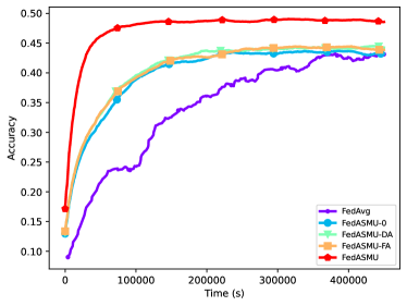
(a) LeNet

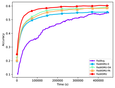
(b) CNN

Figure 2: The accuracy and training time with FedASMU, FedASMU-DA, FedASMU-FA, FedASMU-0, and FedAvg on CIFAR-10.

As shown in Figure 2, we conduct an ablation study with FedASMU-DA, FedASMU-FA, FedASMU-0, and FedAvg. FedASMU-DA represents FedASMU without dynamic model aggregation. FedASMU-FA refers to FedASMU without fresh global model aggregation. FedASMU-0 is FedASMU without the two methods, equivalent to FedAsync with staleness bound. As the dynamic weight adjustment can improve the accuracy, FedASMU outperforms FedASMU-DA (1.38% to 4.32%) and FedASMU-FA outperforms FedASMU-0 (0.65% to 3.04%) in terms of accuracy. As the fresh global model aggregation can reduce the staleness between local models and the global model, FedASMU corresponds to a shorter training time (44.77% to 73.96%) to achieve the target accuracy (0.30 for LeNet and 0.40 for CNN) and higher accuracy (1.75% to 4.71%) compared with FedASMU-FA. In addition, FedASMU-DA leads to better performance (1.04% to 3.41% in terms of accuracy and 15.71% to 19.54% faster) compared with FedASMU-0. Both FedASMU-DA and FedASMU-FA outperform FedAvg in terms of accuracy (0.73% to 3.75%) and efficiency (72.88% to 85.72%). Although FedASMU-0 corresponds to slightly higher accuracy (0.08% to 0.34%) compared with FedAvg, it leads to much higher efficiency (67.84% to 82.26% faster) because of the asynchronous mechanism.

6 Conclusion

In this paper, we propose a novel Asynchronous Stateness-aware Model Update FL framework, i.e., FedASMU, with an asynchronous system model and two novel methods, i.e., a dynamic model aggregation method on the server and an adaptive local model adjustment method on devices. Extensive experimentation reveals significant advantages of FedASMU compared with synchronous and asynchronous baseline approaches in terms of accuracy (0.60% to 23.90% higher) and efficiency (3.54% to 97.98% faster).

Appendix A Appendix

Details for Model Update

In this section, we present the details to calculate the partial deviation for the control parameters on the server and the devices.

Details on the Server

Let us denote the local model for the $(o-1)$-th global model aggregation by $\boldsymbol{w}_{o^{\prime}}^{i}$. Then, we get the version of the global model after aggregating the local model $\boldsymbol{w}_{o^{\prime}}^{i}$ as $o$.

$$\nabla_{\lambda_{o-1}^{i}}\mathcal{F}(\boldsymbol{w}_{o}) =(\frac{\partial\mathcal{F}(\boldsymbol{w}_{o})}{\partial\boldsymbol{w}_{o}})^{\mathrm{T}}\frac{\partial\boldsymbol{w}_{o}}{\partial\lambda_{o-1}^{i}}$$

$$\approx(\frac{\partial\mathcal{F}_{i}(\boldsymbol{w}_{o})}{\partial\boldsymbol{w}_{o}})^{\mathrm{T}}\frac{\partial\boldsymbol{w}_{o}}{\partial\lambda_{o-1}^{i}}$$

$$=g_{i}^{\mathrm{T}}(\boldsymbol{w}_{o})\frac{\partial\boldsymbol{w}_{o}}{\partial\lambda_{o-1}^{i}},$$

where the $\approx$ represents the approximation of the global partial deviation of $\boldsymbol{w}_{o}$ by that on Device $i$.

$$g_{i}^{\mathrm{T}}(\boldsymbol{w}_{o})\approx\frac{\boldsymbol{w}_{o}^{i}-\boldsymbol{w}_{o}}{\eta_{i}\mathcal{L}},$$

where $\boldsymbol{w}_{o}^{i}$ is the updated local model, and $\boldsymbol{w}_{o}$ is the original global model to generate $\boldsymbol{w}_{o}^{i}$. The calculation of $g_{i}^{\mathrm{T}}(\boldsymbol{w}_{o})$ does not incur extra communication.

$$\boldsymbol{w}_{o} =(1-\alpha^{i}_{o-1})\boldsymbol{w}_{o-1}+\alpha^{i}_{o-1}\boldsymbol{w}_{o^{\prime}}^{i}$$

$$=\boldsymbol{w}_{o-1}+\alpha^{i}_{o-1}(\boldsymbol{w}_{o^{\prime}}^{i}-\boldsymbol{w}_{o-1}),$$

where $\boldsymbol{w}_{o-1}^{i}$ and $\boldsymbol{w}_{o-1}$ are independent with $\lambda^{i}_{o-1}$. Thus, we have:

$$\frac{\partial\boldsymbol{w}_{o}}{\partial\lambda_{o-1}^{i}} =\frac{\partial(\boldsymbol{w}_{o-1}+\alpha^{i}_{o-1}(\boldsymbol{w}_{o^{\prime}}^{i}-\boldsymbol{w}_{o-1}))}{\partial\lambda_{o-1}^{i}}$$

$$=(\boldsymbol{w}_{o^{\prime}}^{i}-\boldsymbol{w}_{o-1})\frac{\partial\alpha^{i}_{o-1}}{\partial\lambda_{o-1}^{i}}.$$

After elaborating $\alpha^{i}_{o-1}$, we have:

$$\frac{\partial\alpha^{i}_{o-1}}{\partial\lambda_{o-1}^{i}} =\frac{\partial(1-(1+\mu_{\alpha}\xi^{i}_{o-1})^{(-1)})}{\partial\lambda_{o-1}^{i}}$$

$$=\frac{\mu_{\alpha}}{(1+\mu_{\alpha}\xi^{i}_{o-1})^{2}}\frac{\partial\xi^{i}_{o-1}}{\partial\lambda_{o-1}^{i}}$$

$$=\frac{\mu_{\alpha}}{(1+\mu_{\alpha}\xi^{i}_{o-1})^{2}}\frac{1}{\sqrt{o-1}(o-o^{\prime})^{\sigma^{i}_{o-1}}},$$

where $\xi^{i}_{o-1}$ represents $\xi^{i}_{o-1}(o^{\prime})$ with $o^{\prime}$ representing the version of the original global model to generate updated local model $\boldsymbol{w}_{o^{\prime}}^{i}$ at the $(o-1)$-th global round. Finally, we can calculate the partial deviation of the loss function in terms of $\lambda_{o-1}^{i}$:

$$\nabla_{\lambda^{i}_{o-1}}\mathcal{F}(\boldsymbol{w}_{o})\approx\frac{\mu_{\alpha}(\boldsymbol{w}_{o}^{i}-\boldsymbol{w}_{o})(\boldsymbol{w}_{o^{\prime}}^{i}-\boldsymbol{w}_{o-1})}{\eta_{i}\mathcal{L}\sqrt{o-1}(1+\mu_{\alpha}\xi^{i}_{o-1})^{2}(o-o^{\prime})^{\sigma^{i}_{o-1}}}.$$

Similarly, we can get the partial deviation of the loss function in terms of $\sigma_{o-1}^{i}$ and $\iota_{o-1}^{i}$:

$$\nabla_{\sigma^{i}_{o-1}}\mathcal{F}(\boldsymbol{w}_{o}) \approx\frac{\mu_{\alpha}\ln(\sigma^{i}_{o-1})(\boldsymbol{w}_{o}-\boldsymbol{w}_{o}^{i})(\boldsymbol{w}_{o^{\prime}}^{i}-\boldsymbol{w}_{o-1})}{\eta_{i}\mathcal{L}\sqrt{o-1}(1+\mu_{\alpha}\xi^{i}_{o-1})^{2}(o-o^{\prime})^{\sigma^{i}_{o-1}}},$$

$$\nabla_{\iota^{i}_{o-1}}\mathcal{F}(\boldsymbol{w}_{o}) \approx\frac{\mu_{\alpha}(\boldsymbol{w}_{o}^{i}-\boldsymbol{w}_{o})(\boldsymbol{w}_{o^{\prime}}^{i}-\boldsymbol{w}_{o-1})}{\eta_{i}\mathcal{L}(1+\mu_{\alpha}\xi^{i}_{o-1})^{2}}.$$

Details on the Devices

$$\nabla_{\gamma^{i}_{t_{i}-1}}\mathcal{F}_{i}(\boldsymbol{w}_{o,l}^{b},\zeta_{l-1}) =(\frac{\partial\mathcal{F}_{i}(\boldsymbol{w}_{o,l}^{b},\zeta_{l-1})}{\partial\boldsymbol{w}_{o,l}^{b}})^{\mathrm{T}}\frac{\partial\boldsymbol{w}_{o,l}^{b}}{\partial\gamma_{t_{i}-1}^{i}}$$

$$=g_{o,l}^{\mathrm{T}}(\boldsymbol{w}_{o,l}^{b})\frac{\partial\boldsymbol{w}_{o,l}^{b}}{\partial\gamma_{t_{i}-1}^{i}},$$

where $g_{o,l}^{\mathrm{T}}(\boldsymbol{w}_{o,l}^{b})$ is the local gradient on Device $i$ with $\boldsymbol{w}_{o,l}^{b}$ and $\zeta_{l-1}$.

$$\boldsymbol{w}_{o,l}^{b} =(1-\beta^{i}_{t_{i}-1})\boldsymbol{w}_{o,l}^{a}+\beta^{i}_{t_{i}-1}\boldsymbol{w}_{g}$$

$$=\boldsymbol{w}_{o,l}^{a}+\beta^{i}_{t_{i}-1}(\boldsymbol{w}_{g}-\boldsymbol{w}_{o,l}^{a}),$$

where $\boldsymbol{w}_{g}$ and $\boldsymbol{w}_{o,l}^{a}$ are independent with $\gamma_{t_{i}-1}^{i}$. Then, we have:

$$\frac{\partial\boldsymbol{w}_{o,l}^{b}}{\partial\gamma_{t_{i}-1}^{i}} =\frac{\partial(\boldsymbol{w}_{o,l}^{a}+\beta^{i}_{t_{i}-1}(\boldsymbol{w}_{g}-\boldsymbol{w}_{o,l}^{a}))}{\partial\gamma_{t_{i}-1}^{i}}$$

$$=(\boldsymbol{w}_{g}-\boldsymbol{w}_{o,l}^{a})\frac{\partial\beta^{i}_{t_{i}-1}}{\partial\gamma_{t_{i}-1}^{i}}.$$

After elaborating $\beta^{i}_{t_{i}-1}$, we have:

$$\frac{\partial\beta^{i}_{t_{i}-1}}{\partial\gamma_{t_{i}-1}^{i}} =\frac{\partial(1-(1+\mu_{\beta}\phi^{i}_{t_{i}-1})^{-1})}{\partial\gamma_{t_{i}-1}^{i}}$$

$$=\frac{\mu_{\beta}}{(1+\mu_{\beta}\phi^{i}_{t_{i}-1})^{2}}\frac{\partial\phi^{i}_{t_{i}-1}}{\partial\gamma_{t_{i}-1}^{i}}$$

$$=\frac{\mu_{\beta}}{\sqrt{g}(1+\mu_{\beta}\phi^{i}_{t_{i}-1})^{2}}(1-\frac{\upsilon^{i}_{t_{i}-1}}{\sqrt{g-o+1}}),$$

where $\phi^{i}_{t_{i}-1}$ represents $\phi^{i}_{t_{i}-1}(g,o)$. Finally, we can calculate the partial deviation of the loss function in terms of $\gamma_{t_{i}-1}^{i}$:

$$\nabla_{\gamma^{i}_{t_{i}-1}}\mathcal{F}_{i}(\boldsymbol{w}_{o,l}^{b},\zeta_{l-1})$$

$$={} (\boldsymbol{w}_{g}-\boldsymbol{w}_{o,l}^{a})\frac{\mu_{\beta}g_{o,l}^{\mathrm{T}}(\boldsymbol{w}_{o,l}^{b})}{\sqrt{g}(1+\mu_{\beta}\phi^{i}_{t_{i}-1})^{2}}(1-\frac{\upsilon^{i}_{t_{i}-1}}{\sqrt{g-o+1}}).$$

Similarly, we can get the partial deviation of the loss function in terms of $\upsilon^{i}_{t_{i}-1}$:

$$\nabla_{\upsilon^{i}_{t_{i}-1}}\mathcal{F}_{i}(\boldsymbol{w}_{o,l}^{b},\zeta_{l-1}) =\frac{\mu_{\beta}\gamma^{i}_{t_{i}-1}g_{o,l}^{\mathrm{T}}(\boldsymbol{w}_{o,l}^{b})(\boldsymbol{w}_{o,l}^{a}-\boldsymbol{w}_{g})}{\sqrt{g}\sqrt{g-o+1}(1+\mu_{\beta}\phi^{i}_{t_{i}-1})^{2}}.$$

Convergence Analysis

In this section, we present the assumptions, the convergence guarantees of FedASMU, and the proof.

Assumption 1.

($L$-smoothness) The loss function $\mathcal{F}_{i}$ is differentiable and $L$-smooth for each device $i\in\mathcal{M}$ and $\forall x,y$, $\mathcal{F}_{i}(y)-\mathcal{F}_{i}(x)\leq\left\langle\nabla\mathcal{F}_{i}(x),y-x\right\rangle+\frac{L}{2}\|y-x\|^{2}$ with $L>0$.

Assumption 2.

($\mu$-strongly convex) The loss function $\mathcal{F}_{i}$ is $\mu$-strongly convex for each device $i\in\mathcal{M}$: $\langle\nabla\mathcal{F}_{i}(x)-\nabla\mathcal{F}_{i}(y),x-y\rangle\geq\mu\parallel x-y\parallel^{2}$ with $\mu>0$.

Assumption 3.

(Unbiased sampling) The local sampling is unbiased and the local gradients are unbiased stochastic gradients $\mathbb{E}_{\zeta_{l}\sim\mathcal{D}_{i}}[\nabla\mathcal{F}_{i}(\boldsymbol{w}_{o,l};\zeta_{l})]=\nabla\mathcal{F}_{i}(\boldsymbol{w}_{o,l})$.

Assumption 4.

(Bounded local gradient) The stochastic gradients are bounded on each device $i\in\mathcal{M}$: $\mathbb{E}_{\zeta_{l}\sim\mathcal{D}_{i}}\parallel\nabla\mathcal{F}_{i}(\boldsymbol{w}_{o,l};\zeta_{l})\parallel^{2}\leq{\mathcal{G}^{2}}$.

Assumption 5.

(Bounded local variance) The variance of local stochastic gradients are bounded on each device $i\in\mathcal{M}$ is bounded: $\mathbb{E}_{\zeta_{l}\sim\mathcal{D}_{i}}\parallel\nabla\mathcal{F}_{i}(\boldsymbol{w}_{o,l};\zeta_{l})-\mathcal{F}(\boldsymbol{w}_{o,l})\parallel^{2}\leq{\mathcal{V}^{2}}$.

Theorem 1.

Let Assumptions 1 - 5 hold, after $T$ global updates, FedASMU converges to a critical point:

$$\min_{t=0}^{T}{\mathbb{E}}\parallel\nabla\mathcal{F}(\boldsymbol{w}_{o,l})\parallel^{2}$$

$$\leq~{} \frac{2{\mathbb{E}}\left[\mathcal{F}(\boldsymbol{w}_{0})-\mathcal{F}(\boldsymbol{w}_{T})\right]}{\alpha_{min}\mathcal{L}_{min}^{3}}+{\mathcal{O}}\left(\frac{L\mathcal{G}^{2}\mathcal{L}_{max}}{\mathcal{L}_{min}^{3}}\right)$$

$$\quad+{\mathcal{O}}\left(\frac{\mathcal{L}^{i}\mathcal{V}^{2}}{\mathcal{L}_{min}^{7}}\right)+{\mathcal{O}}\left(\frac{\tau\mathcal{G}^{2}\mathcal{L}_{max}}{\mathcal{L}_{min}^{7}}\right)$$

$$\quad+{\mathcal{O}}\left(\frac{\mathcal{G}^{2}\mathcal{L}_{max}}{\mathcal{L}_{min}^{3}}\right)+{\mathcal{O}}\left(\frac{L\mathcal{G}^{2}\mathcal{L}_{max}}{\mathcal{L}_{min}^{3}}\right)$$

$$+{\mathcal{O}}\left(\frac{L\tau^{2}\mathcal{G}^{2}\mathcal{L}_{max}^{2}}{\mathcal{L}_{min}^{3}}\right)+{\mathcal{O}}\left(\frac{L\tau^{2}\mathcal{G}^{2}\mathcal{L}_{max}^{2}}{\mathcal{L}_{min}^{3}}\right),$$

where $\alpha_{min}\leq\alpha_{t}^{i}$, $\mathcal{L}_{min}\leq\mathcal{L}_{t}\leq\mathcal{L}_{max}$, $\eta_{i}=\frac{1}{\sqrt{T}}$, $\forall i\in\mathcal{M}$, and $T=\mathcal{L}_{min}^{6}$.

Proof.

First, we denote the optimal model by $\boldsymbol{w}^{*}$, the new fresh global gradient is not received at the $l$-th local epoch, and we have the following inequality with the vanilla SGD in devices:

$$~{}{\mathbb{E}}\left[\mathcal{F}(\boldsymbol{w}_{o,l})-\mathcal{F}(\boldsymbol{w}^{*})\right]$$

$$= ~{}{\mathbb{E}}_{\zeta_{l-1}\sim\mathcal{D}_{i}}\left[\mathcal{F}(\boldsymbol{w}_{o,l-1}-\eta_{i}\nabla\mathcal{F}_{i}(\boldsymbol{w}_{o,l-1},\zeta_{l-1}))-\mathcal{F}(\boldsymbol{w}^{*})\right]$$

$$\leq ~{}\mathcal{F}(\boldsymbol{w}_{o,l-1})-F(\boldsymbol{w}^{*})$$

$$\quad-\eta_{i}{\mathbb{E}}_{\zeta_{l-1}\sim\mathcal{D}_{i}}\left[\left\langle\nabla\mathcal{F}(\boldsymbol{w}_{o,l-1}),\nabla\mathcal{F}_{i}(\boldsymbol{w}_{o,l-1},\zeta_{l-1})\right\rangle\right]$$

$$\quad+\frac{L\eta_{i}^{2}}{2}{\mathbb{E}}_{\zeta_{l-1}\sim\mathcal{D}_{i}}\left[\|\nabla\mathcal{F}_{i}(\boldsymbol{w}_{o,l-1},\zeta_{l-1})\|^{2}\right]$$

$$\leq ~{}\mathcal{F}(\boldsymbol{w}_{o,l-1})-F(\boldsymbol{w}^{*})+\frac{L\eta_{i}^{2}\mathcal{G}^{2}}{2}$$

$$\quad-\eta_{i}\underbrace{{\mathbb{E}}_{\zeta_{l-1}\sim\mathcal{D}_{i}}\left[\left\langle\nabla\mathcal{F}(\boldsymbol{w}_{o,l-1}),\nabla\mathcal{F}_{i}(\boldsymbol{w}_{o,l-1},\zeta_{l-1})\right\rangle\right]}_{A},$$ (1)

where the first inequality comes from $L$-smoothness and the second one is from bounded local gradient. Then, we focus on $A$.

$$~{}\mathbb{E}_{\zeta_{l-1}\sim\mathcal{D}_{i}}\parallel\nabla\mathcal{F}_{i}(\boldsymbol{w}_{o,l-1};\zeta_{l-1})-\nabla\mathcal{F}(\boldsymbol{w}_{o,l-1})\parallel^{2}$$

$$= ~{}{\mathbb{E}}\parallel\nabla\mathcal{F}(\boldsymbol{w}_{o,l-1})\parallel^{2}-2A$$

$$\quad+~{}\mathbb{E}_{\zeta_{l-1}\sim\mathcal{D}_{i}}\parallel\nabla\mathcal{F}_{i}(\boldsymbol{w}_{o,l-1};\zeta_{l-1})\parallel^{2}.$$

Based on the bounded local variance assumption, we have:

$$\mathcal{V}^{2}=~{} {\mathbb{E}}\parallel\nabla\mathcal{F}(\boldsymbol{w}_{o,l-1})\parallel^{2}-2A$$

$$\quad+~{}\mathbb{E}_{\zeta_{l-1}\sim\mathcal{D}_{i}}\parallel\nabla\mathcal{F}_{i}(\boldsymbol{w}_{o,l-1};\zeta_{l-1})\parallel^{2},$$

and we can get $A$:

$$A= \frac{1}{2}({\mathbb{E}}\parallel\nabla\mathcal{F}(\boldsymbol{w}_{o,l-1})\parallel^{2}-~{}\mathcal{V}^{2}$$

$$\quad+~{}\mathbb{E}_{\zeta_{l-1}\sim\mathcal{D}_{i}}\parallel\nabla\mathcal{F}_{i}(\boldsymbol{w}_{o,l-1};\zeta_{l-1})\parallel^{2}),$$

Plug this into Formula 1, and we have:

$$~{}{\mathbb{E}}\left[\mathcal{F}(\boldsymbol{w}_{o,l})-\mathcal{F}(\boldsymbol{w}^{*})\right]$$

$$\leq ~{}\mathcal{F}(\boldsymbol{w}_{o,l-1})-F(\boldsymbol{w}^{*})+\frac{L\eta_{i}^{2}\mathcal{G}^{2}}{2}$$

$$\quad-\frac{\eta_{i}}{2}({\mathbb{E}}\parallel\nabla\mathcal{F}(\boldsymbol{w}_{o,l-1})\parallel^{2}-\mathcal{V}^{2}$$

$$\quad+~{}\mathbb{E}_{\zeta_{l-1}\sim\mathcal{D}_{i}}\parallel\nabla\mathcal{F}_{i}(\boldsymbol{w}_{o,l-1};\zeta_{l-1})\parallel^{2})$$

$$\leq ~{}\mathcal{F}(\boldsymbol{w}_{o,l-1})-F(\boldsymbol{w}^{*})-\frac{\eta_{i}}{2}{\mathbb{E}}\parallel\nabla\mathcal{F}(\boldsymbol{w}_{o,l-1})\parallel^{2}$$

$$\quad+\frac{L\eta_{i}^{2}\mathcal{G}^{2}+\eta_{i}\mathcal{V}^{2}}{2},$$

where the second inequality is because $\mathbb{E}_{\zeta_{l-1}\sim\mathcal{D}_{i}}\parallel\nabla\mathcal{F}_{i}(\boldsymbol{w}_{o,l-1};\zeta_{l-1})\parallel^{2}\geq 0$. By rearranging the terms and telescoping, we have:

$${\mathbb{E}}\parallel\nabla\mathcal{F}(\boldsymbol{w}_{o,l-1})\parallel^{2}\leq \frac{2}{\eta_{i}}{\mathbb{E}}\left[\mathcal{F}(\boldsymbol{w}_{o,l-1})-\mathcal{F}(\boldsymbol{w}_{o,l})\right]$$

$$\quad+L\eta_{i}\mathcal{G}^{2}+\mathcal{V}^{2}.$$

However, when the fresh global model $\boldsymbol{w}_{g}$ is received right at the $l^{*}$-th local epoch, we have:

$${\mathbb{E}}\parallel\nabla\mathcal{F}(\boldsymbol{w}_{o,l^{*}})\parallel^{2}$$

$$\leq \frac{2}{\eta_{i}}{\mathbb{E}}\left[\mathcal{F}(\boldsymbol{w}_{o,l^{*}-1}^{a})-\mathcal{F}(\boldsymbol{w}_{o,l^{*}})\right]+L\eta_{i}\mathcal{G}^{2}+\mathcal{V}^{2}$$

$$= \frac{2}{\eta_{i}}{\mathbb{E}}\left[\mathcal{F}((1-\beta^{i}_{t_{i}-1})\boldsymbol{w}_{o,l^{*}-1}^{b}+\beta^{i}_{t_{i}-1}\boldsymbol{w}_{g})-\mathcal{F}(\boldsymbol{w}_{o,l^{*}})\right]$$

$$\quad+L\eta_{i}\mathcal{G}^{2}+\mathcal{V}^{2}$$

$$\leq \frac{2}{\eta_{i}}{\mathbb{E}}\left[(1-\beta^{i}_{t_{i}-1})\mathcal{F}(\boldsymbol{w}_{o,l^{*}-1}^{b})+\beta^{i}_{t_{i}-1}\mathcal{F}(\boldsymbol{w}_{g})-\mathcal{F}(\boldsymbol{w}_{o,l^{*}})\right]$$

$$\quad+L\eta_{i}\mathcal{G}^{2}+\mathcal{V}^{2}$$

$$= \frac{2}{\eta_{i}}{\mathbb{E}}\left[(1-\beta^{i}_{t_{i}-1})\mathcal{F}(\boldsymbol{w}_{o,l^{*}-1})+\beta^{i}_{t_{i}-1}\mathcal{F}(\boldsymbol{w}_{g})-\mathcal{F}(\boldsymbol{w}_{o,l^{*}})\right]$$

$$\quad+L\eta_{i}\mathcal{G}^{2}+\mathcal{V}^{2}$$

$$= \frac{2}{\eta_{i}}{\mathbb{E}}\left[\mathcal{F}(\boldsymbol{w}_{o,l^{*}-1})-\mathcal{F}(\boldsymbol{w}_{o,l^{*}})\right]$$

$$\quad+\frac{2\beta^{i}_{t_{i}-1}}{\eta_{i}}{\mathbb{E}}\left[\mathcal{F}(\boldsymbol{w}_{g})-\mathcal{F}(\boldsymbol{w}_{o,l^{*}-1})\right]$$

$$\quad+L\eta_{i}\mathcal{G}^{2}+\mathcal{V}^{2}$$ (2)

where the second inequality is because of convexity of $\mathcal{F}(\cdot)$. Then, we can get:

$$~{}\sum_{l=1}^{\mathcal{L}^{i}}{\mathbb{E}}\parallel\nabla\mathcal{F}(\boldsymbol{w}_{o,l})\parallel^{2}$$

$$\leq ~{}\frac{2}{\eta_{i}}{\mathbb{E}}\left[\mathcal{F}(\boldsymbol{w}_{o,0})-\mathcal{F}(\boldsymbol{w}_{o,\mathcal{L}^{i}})\right]+\mathcal{L}^{i}(L\eta_{i}\mathcal{G}^{2}+\mathcal{V}^{2})$$

$$\quad+\frac{2\beta^{i}_{t_{i}-1}}{\eta_{i}}{\mathbb{E}}\left[\mathcal{F}(\boldsymbol{w}_{g})-\mathcal{F}(\boldsymbol{w}_{o,l^{*}-1})\right]$$

$$= ~{}\frac{2}{\eta_{i}}{\mathbb{E}}\left[\mathcal{F}(\boldsymbol{w}_{o})-\mathcal{F}(\boldsymbol{w}_{o}^{i})\right]+\mathcal{L}^{i}(L\eta_{i}\mathcal{G}^{2}+\mathcal{V}^{2})$$

$$\quad+\frac{2\beta^{i}_{t_{i}-1}}{\eta_{i}}{\mathbb{E}}\left[\mathcal{F}(\boldsymbol{w}_{g})-\mathcal{F}(\boldsymbol{w}_{o,l^{*}-1})\right]$$

$$= ~{}\frac{2}{\eta_{i}}\underbrace{{\mathbb{E}}\left[\mathcal{F}(\boldsymbol{w}_{o})-\mathcal{F}(\boldsymbol{w}_{o}^{i})\right]}_{B}+\mathcal{L}^{i}(L\eta_{i}\mathcal{G}^{2}+\mathcal{V}^{2})$$

$$\quad+\frac{2}{\eta_{i}}\beta^{i}_{t_{i}-1}\underbrace{{\mathbb{E}}\left[\mathcal{F}(\boldsymbol{w}_{o,0})-\mathcal{F}(\boldsymbol{w}_{o,l^{*}-1})\right]}_{C}$$

$$\quad+\frac{2}{\eta_{i}}\beta^{i}_{t_{i}-1}\underbrace{{\mathbb{E}}\left[\mathcal{F}(\boldsymbol{w}_{g})-\mathcal{F}(\boldsymbol{w}_{o})\right]}_{D}.$$

First, we focus on the calculation of $B$.

$${\mathbb{E}}\left[\mathcal{F}(\boldsymbol{w}_{t+1})-\mathcal{F}(\boldsymbol{w}_{t})\right]$$

$$= ~{}{\mathbb{E}}\left[\mathcal{F}((1-\alpha^{i}_{t})\boldsymbol{w}_{t}+\alpha^{i}_{t}\boldsymbol{w}_{o}^{i})-\mathcal{F}(\boldsymbol{w}_{t})\right]$$

$$\leq ~{}{\mathbb{E}}\left[(1-\alpha^{i}_{t})\mathcal{F}(\boldsymbol{w}_{t})+\alpha^{i}_{t}\mathcal{F}(\boldsymbol{w}_{o}^{i})-\mathcal{F}(\boldsymbol{w}_{t})\right]$$

$$= ~{}\alpha^{i}_{t}{\mathbb{E}}\left[\mathcal{F}(\boldsymbol{w}_{o}^{i})-\mathcal{F}(\boldsymbol{w}_{t})\right]$$

$$= ~{}\alpha^{i}_{t}{\mathbb{E}}\left[\mathcal{F}(\boldsymbol{w}_{o}^{i})-\mathcal{F}(\boldsymbol{w}_{o})+\mathcal{F}(\boldsymbol{w}_{o})-\mathcal{F}(\boldsymbol{w}_{t})\right],$$

where the inequility is because $\mathcal{F}(\cdot)$ is convex. Then, we have:

$$~{}{\mathbb{E}}\left[\mathcal{F}(\boldsymbol{w}_{t+1})-\mathcal{F}(\boldsymbol{w}_{t})\right]$$

$$\leq ~{}\alpha^{i}_{t}{\mathbb{E}}\left[\mathcal{F}(\boldsymbol{w}_{o}^{i})-\mathcal{F}(\boldsymbol{w}_{o})+\mathcal{F}(\boldsymbol{w}_{o})-\mathcal{F}(\boldsymbol{w}_{t})\right].$$

And, we can get:

$$~{}{\mathbb{E}}\left[\mathcal{F}(\boldsymbol{w}_{o})-\mathcal{F}(\boldsymbol{w}_{o}^{i})\right]$$

$$\leq ~{}\frac{1}{\alpha^{i}_{t}}{\mathbb{E}}\left[\mathcal{F}(\boldsymbol{w}_{t})-\mathcal{F}(\boldsymbol{w}_{t+1})\right]+{\mathbb{E}}\left[\mathcal{F}(\boldsymbol{w}_{o})-\mathcal{F}(\boldsymbol{w}_{t})\right].$$

Using $L$-smoothness, we have:

$$~{}{\mathbb{E}}\left[\mathcal{F}(\boldsymbol{w}_{o})-\mathcal{F}(\boldsymbol{w}_{t})\right]$$

$$\leq ~{}\left\langle\nabla\mathcal{F}(\boldsymbol{w}_{t}),\boldsymbol{w}_{o}-\boldsymbol{w}_{t}\right\rangle+\frac{L}{2}\parallel\boldsymbol{w}_{o}-\boldsymbol{w}_{t}\parallel^{2}$$

$$\leq ~{}\parallel\nabla\mathcal{F}(\boldsymbol{w}_{t})\parallel\parallel\boldsymbol{w}_{o}-\boldsymbol{w}_{t}\parallel+\frac{L}{2}\parallel\boldsymbol{w}_{o}-\boldsymbol{w}_{t}\parallel^{2}$$

As the fresh global model is incurred to reduce the difference between the local model and the global model, the difference between the global models of two versions is because of the local updates. Then, we have the upper bound of local updates:

$$~{}\parallel\boldsymbol{w}_{o,0}-\boldsymbol{w}_{o,\mathcal{L}^{i}}\parallel$$

$$\leq ~{}\parallel\boldsymbol{w}_{o,0}-\boldsymbol{w}_{o,1}\parallel+\parallel\boldsymbol{w}_{o,1}-\boldsymbol{w}_{o,2}\parallel+\cdots$$

$$\quad+\parallel\boldsymbol{w}_{o,\mathcal{L}^{i}-1}-\boldsymbol{w}_{o,\mathcal{L}^{i}}\parallel$$

$$\leq ~{}\eta_{i}\mathcal{L}^{i}\mathcal{G}.$$

And, we get:

$$\parallel\boldsymbol{w}_{o}-\boldsymbol{w}_{o+1}\parallel =\parallel\boldsymbol{w}_{o}-(1-\alpha_{t}^{i})\boldsymbol{w}_{o}-\alpha_{t}^{i}\boldsymbol{w}_{o,\mathcal{L}^{i}}\parallel$$

$$=\alpha_{t}^{i}\parallel\boldsymbol{w}_{o,0}-\boldsymbol{w}_{o,\mathcal{L}^{i}}\parallel$$

$$\leq\eta_{i}\alpha_{t}^{i}\mathcal{L}\mathcal{G}.$$

Thus, we have:

$$\parallel\boldsymbol{w}_{o}-\boldsymbol{w}_{t}\parallel \leq(t-o+1)\eta_{i}\alpha_{t}^{i}\mathcal{L}^{i}\mathcal{G},$$

where $t-o+1\leq\tau$ because of staleness bound. Then, we can get:

$$\parallel\boldsymbol{w}_{o}-\boldsymbol{w}_{t}\parallel \leq\tau\eta_{i}\alpha_{t}^{i}\mathcal{L}^{i}\mathcal{G}.$$

Then, we have:

$$~{}{\mathbb{E}}\left[\mathcal{F}(\boldsymbol{w}_{o})-\mathcal{F}(\boldsymbol{w}_{t})\right]$$

$$\leq ~{}\parallel\nabla\mathcal{F}(\boldsymbol{w}_{t})\parallel\parallel\boldsymbol{w}_{o}-\boldsymbol{w}_{t}\parallel+\frac{L}{2}\parallel\boldsymbol{w}_{o}-\boldsymbol{w}_{t}\parallel^{2}$$

$$\leq\tau\eta_{i}\alpha_{t}^{i}\mathcal{L}^{i}\mathcal{G}^{2}+\frac{L}{2}(\tau\eta_{i}\alpha_{t}^{i}\mathcal{L}^{i}\mathcal{G})^{2}.$$

And, we can calculate $B$:

$$B\leq \frac{1}{\alpha^{i}_{t}}{\mathbb{E}}\left[\mathcal{F}(\boldsymbol{w}_{t})-\mathcal{F}(\boldsymbol{w}_{t+1})\right]+\tau\eta_{i}\alpha_{t}^{i}\mathcal{L}\mathcal{G}^{2}$$

$$\quad+\frac{L}{2}(\tau\eta_{i}\alpha_{t}^{i}\mathcal{L}\mathcal{G})^{2}.$$

Now, we focus on the calculation of $C$. Based on the convexity of $\mathcal{F}(\cdot)$, we have:

$$~{}{\mathbb{E}}\left[\mathcal{F}(\boldsymbol{w}_{o,l-1})-\mathcal{F}(\boldsymbol{w}_{o,l})\right]$$

$$\leq ~{}\left\langle\nabla\mathcal{F}(\boldsymbol{w}_{o,l}),\boldsymbol{w}_{o,l-1}-\boldsymbol{w}_{o,l}\right\rangle+\frac{L}{2}\parallel\boldsymbol{w}_{o,l-1}-\boldsymbol{w}_{o,l}\parallel^{2}$$

$$= ~{}\eta_{i}\left\langle\nabla\mathcal{F}(\boldsymbol{w}_{o,l}),\nabla\mathcal{F}_{i}(\boldsymbol{w}_{o,l-1})\right\rangle+\frac{L\eta_{i}^{2}}{2}\parallel\nabla\mathcal{F}_{i}(\boldsymbol{w}_{o,l-1})\parallel^{2}$$

$$\leq ~{}\frac{\eta_{i}}{2}(\parallel\nabla\mathcal{F}(\boldsymbol{w}_{o,l})\parallel^{2}+\parallel\nabla\mathcal{F}_{i}(\boldsymbol{w}_{o,l-1})\parallel^{2})+\frac{L\eta_{i}^{2}\mathcal{G}^{2}}{2}$$

$$\leq ~{}\frac{2\eta_{i}+L\eta_{i}^{2}}{2}\mathcal{G}^{2},$$

Then, we can have:

$$C= ~{}{\mathbb{E}}\left[\mathcal{F}(\boldsymbol{w}_{o,0})-\mathcal{F}(\boldsymbol{w}_{o,l^{*}-1})\right]$$

$$\leq ~{}\frac{2\eta_{i}+L\eta_{i}^{2}}{2}(l^{*}-1)\mathcal{G}^{2}$$

$$\leq ~{}\frac{2\eta_{i}+L\eta_{i}^{2}}{2}\mathcal{L}^{i}\mathcal{G}^{2}.$$

Next, we focus on the calculation of $D$.

$$D \leq\left\langle\nabla\mathcal{F}(\boldsymbol{w}_{o}),\boldsymbol{w}_{g}-\boldsymbol{w}_{o}\right\rangle+\frac{L}{2}\|\boldsymbol{w}_{g}-\boldsymbol{w}_{o}\|^{2}$$

$$\leq\|\nabla\mathcal{F}(\boldsymbol{w}_{o})\|\|\boldsymbol{w}_{g}-\boldsymbol{w}_{o}\|+\frac{L}{2}\|\boldsymbol{w}_{g}-\boldsymbol{w}_{o}\|^{2}.$$

As $(g-o\leq\tau)$ because of staleness bound, we have:

$$\parallel\boldsymbol{w}_{g}-\boldsymbol{w}_{o}\parallel\leq(g-o)\eta_{i}\alpha_{t}^{i}\mathcal{L}\mathcal{G}\leq\tau\eta_{i}\alpha_{t}^{i}\mathcal{L}\mathcal{G}.$$

Then, we have:

$$D \leq\|\nabla\mathcal{F}(\boldsymbol{w}_{o})\|\|\boldsymbol{w}_{g}-\boldsymbol{w}_{o}\|+\frac{L}{2}\|\boldsymbol{w}_{g}-\boldsymbol{w}_{o}\|^{2}$$

$$\leq\tau\eta_{i}\alpha_{t}^{i}\mathcal{L}\mathcal{G}^{2}+\frac{L}{2}(\tau\eta_{i}\alpha_{t}^{i}\mathcal{L}\mathcal{G})^{2}.$$

By rearranging the terms, we have

$$~{}\sum_{l=1}^{\mathcal{L}^{i}}{\mathbb{E}}\parallel\nabla\mathcal{F}(\boldsymbol{w}_{o,l})\parallel^{2}$$

$$\leq ~{}\frac{2}{\eta_{i}}\underbrace{{\mathbb{E}}\left[\mathcal{F}(\boldsymbol{w}_{o})-\mathcal{F}(\boldsymbol{w}_{o}^{i})\right]}_{B}$$

$$\quad+\frac{2}{\eta_{i}}\beta^{i}_{t_{i}-1}\underbrace{{\mathbb{E}}\left[\mathcal{F}(\boldsymbol{w}_{o,0})-\mathcal{F}(\boldsymbol{w}_{o,l^{*}-1})\right]}_{C}$$

$$\quad+\frac{2}{\eta_{i}}\beta^{i}_{t_{i}-1}\underbrace{{\mathbb{E}}\left[\mathcal{F}(\boldsymbol{w}_{g})-\mathcal{F}(\boldsymbol{w}_{o})\right]}_{D}+\mathcal{L}^{i}(L\eta_{i}\mathcal{G}^{2}+\mathcal{V}^{2})$$

$$\leq ~{}\frac{2}{\eta_{i}}(\frac{1}{\alpha^{i}_{t}}{\mathbb{E}}\left[\mathcal{F}(\boldsymbol{w}_{t})-\mathcal{F}(\boldsymbol{w}_{t+1})\right])$$

$$\quad+\frac{2}{\eta_{i}}(\tau\eta_{i}\alpha_{t}^{i}\mathcal{L}^{i}\mathcal{G}^{2}+\frac{L}{2}(\tau\eta_{i}\alpha_{t}^{i}\mathcal{L}^{i}\mathcal{G})^{2})$$

$$\quad+\beta^{i}_{t_{i}-1}\frac{2\eta_{i}+L\eta_{i}^{2}}{2}\mathcal{L}^{i}\mathcal{G}^{2}$$

$$\quad+\beta^{i}_{t_{i}-1}(\tau\eta_{i}\alpha_{t}^{i}\mathcal{L}^{i}\mathcal{G}^{2}+\frac{L}{2}(\tau\eta_{i}\alpha_{t}^{i}\mathcal{L}^{i}\mathcal{G})^{2})$$

$$\quad+\mathcal{L}^{i}(L\eta_{i}\mathcal{G}^{2}+\mathcal{V}^{2})$$

$$= ~{}\frac{2{\mathbb{E}}\left[\mathcal{F}(\boldsymbol{w}_{t})-\mathcal{F}(\boldsymbol{w}_{t+1})\right]}{\alpha^{i}_{t}\eta_{i}}+\mathcal{L}^{i}\mathcal{V}^{2}$$

$$\quad+\frac{\beta^{i}_{t_{i}-1}+\tau^{2}(\alpha_{t}^{i})^{2}\mathcal{L}^{i}}{2}L\mathcal{L}^{i}\eta_{i}^{2}\mathcal{G}^{2}$$

$$\quad+(2\tau\alpha_{t}^{i}+L\tau^{2}\eta_{i}(\alpha_{t}^{i})^{2}\mathcal{L}^{i}+\beta^{i}_{t_{i}-1}\eta_{i}$$

$$\quad+\beta^{i}_{t_{i}-1}\tau+\eta_{i}\alpha_{t}^{i}+L\eta_{i})\mathcal{L}^{i}\mathcal{G}^{2}.$$

We take $\alpha_{min}\leq\alpha_{t}^{i}\leq 1$ and $0\leq\beta^{i}_{t_{i}-1}\leq 1$ with $\alpha_{min}>0$, we can get:

$$~{}\sum_{l=1}^{\mathcal{L}^{i}}{\mathbb{E}}\parallel\nabla\mathcal{F}(\boldsymbol{w}_{o,l})\parallel^{2}$$

$$\leq ~{}\frac{2{\mathbb{E}}\left[\mathcal{F}(\boldsymbol{w}_{t})-\mathcal{F}(\boldsymbol{w}_{t+1})\right]}{\alpha_{min}\eta_{i}}+\mathcal{L}^{i}\mathcal{V}^{2}+\frac{1+\tau^{2}\mathcal{L}^{i}}{2}L\mathcal{L}^{i}\eta_{i}^{2}\mathcal{G}^{2}$$

$$+(3\tau+L\tau^{2}\eta_{i}\mathcal{L}^{i}+2\eta_{i}+L\eta_{i})\mathcal{L}^{i}\mathcal{G}^{2}.$$

After $T$ global rounds, we have:

$$~{}\frac{1}{\sum_{t=0}^{T}\mathcal{L}_{t}}\sum_{t=0}^{T}\sum_{l=0}^{\mathcal{L}_{t}}{\mathbb{E}}\parallel\nabla\mathcal{F}(\boldsymbol{w}_{o,l})\parallel^{2}$$

$$\leq ~{}\frac{2{\mathbb{E}}\left[\mathcal{F}(\boldsymbol{w}_{0})-\mathcal{F}(\boldsymbol{w}_{T})\right]}{\alpha_{min}\eta_{i}T\mathcal{L}_{min}}+\frac{1+\tau^{2}\mathcal{L}_{max}}{2T\mathcal{L}_{min}}L\mathcal{L}_{max}\eta_{i}\mathcal{G}^{2}$$

$$+\frac{3\tau+L\tau^{2}\eta_{i}\mathcal{L}_{max}+2\eta_{i}+L\eta_{i}}{T\mathcal{L}_{min}}\mathcal{L}_{max}\mathcal{G}^{2}+\frac{\mathcal{L}_{max}\mathcal{V}^{2}}{T\mathcal{L}_{min}},$$

where $\mathcal{L}_{t}$ represents the maximum local epochs within the $t$-th global round with $\mathcal{L}_{min}\leq\mathcal{L}_{t}\leq\mathcal{L}_{max}$. We take $\eta_{i}=\frac{1}{\sqrt{T}}$ and $T=\mathcal{L}_{min}^{6}$, and can get:

$$~{}\frac{1}{\sum_{t=0}^{T}\mathcal{L}_{t}}\sum_{t=0}^{T}\sum_{l=0}^{\mathcal{L}_{t}}{\mathbb{E}}\parallel\nabla\mathcal{F}(\boldsymbol{w}_{o,l})\parallel^{2}$$

$$\leq ~{}\frac{2{\mathbb{E}}\left[\mathcal{F}(\boldsymbol{w}_{0})-\mathcal{F}(\boldsymbol{w}_{T})\right]}{\alpha_{min}\mathcal{L}_{min}^{3}}+\frac{1+\tau^{2}\mathcal{L}_{max}}{2\mathcal{L}_{min}^{3}}L\mathcal{L}_{max}\mathcal{G}^{2}$$

$$\quad+\frac{3\tau\mathcal{L}_{max}\mathcal{G}^{2}+\mathcal{L}^{i}\mathcal{V}^{2}}{\mathcal{L}_{min}^{7}}+\frac{L\tau^{2}\mathcal{L}_{max}+2+L}{\mathcal{L}_{min}^{3}}\mathcal{L}_{max}\mathcal{G}^{2}$$

$$\leq \frac{2{\mathbb{E}}\left[\mathcal{F}(\boldsymbol{w}_{0})-\mathcal{F}(\boldsymbol{w}_{T})\right]}{\alpha_{min}\mathcal{L}_{min}^{3}}+{\mathcal{O}}\left(\frac{L\mathcal{G}^{2}\mathcal{L}_{max}}{\mathcal{L}_{min}^{3}}\right)$$

$$\quad+{\mathcal{O}}\left(\frac{\mathcal{L}^{i}\mathcal{V}^{2}}{\mathcal{L}_{min}^{7}}\right)+{\mathcal{O}}\left(\frac{\tau\mathcal{G}^{2}\mathcal{L}_{max}}{\mathcal{L}_{min}^{7}}\right)$$

$$\quad+{\mathcal{O}}\left(\frac{\mathcal{G}^{2}\mathcal{L}_{max}}{\mathcal{L}_{min}^{3}}\right)+{\mathcal{O}}\left(\frac{L\mathcal{G}^{2}\mathcal{L}_{max}}{\mathcal{L}_{min}^{3}}\right)$$

$$+{\mathcal{O}}\left(\frac{L\tau^{2}\mathcal{G}^{2}\mathcal{L}_{max}^{2}}{\mathcal{L}_{min}^{3}}\right)+{\mathcal{O}}\left(\frac{L\tau^{2}\mathcal{G}^{2}\mathcal{L}_{max}^{2}}{\mathcal{L}_{min}^{3}}\right)$$

∎

Experiment details

Table 3: The network structure of CNN.

Layer (type)	Parameters	Input Layer
conv1(Convolution)	channels=64, kernel_size=2	data
activation1(Activation)	null	conv1
conv2(Convolution)	channels=32, kernel_size=2	activation1
activation2(Activation)	null	conv2
flatten1(Flatten)	null	activation2
dense1(Dense)	units=10	flatten1
softmax(SoftmaxOutput)	null	dense1

In the experiment, we exploit a CNN model with the network structure shown in Table 3. We exploit 44 Tesla V100 GPU cards to simulate the FL environment. We simulate device heterogeneity by considering the variations in local training times, i.e., the training time of the slowest device is five times longer than that of the fastest device, and the training time of each device is independently and randomly sampled within this range. We exploit a learning rate decay for the training process. In addition, we take 500 as the maximum number of epochs for synchronous approaches and 5000 as that of asynchronous approaches. The server triggers one idle task every 5 seconds, with a maximum parallelism constraint, i.e., 10% of the total device number. We fine-tune the hyper-parameters for each approach and report the best one in the paper. The summary of main notations is shown in Table 4 and the values of hyper-parameters are shown in Tables 5 and 6.

Table 4: Summary of main notations.

Notation	Definition
$\mathcal{M}$; $m$	The set of edge devices; the size of $\mathcal{M}$
$\mathcal{D}$; $|\mathcal{D}|$	The global dataset; the size of $\mathcal{D}$
$\mathcal{D}_{i}$; $|\mathcal{D}_{i}|$	The dataset on Device $i$; the size of $\mathcal{D}_{i}$
$\mathcal{F}(\cdot)$; $\mathcal{F}_{i}(\cdot)$	The global loss function; the local loss function on Device $i$
$T$	The maximum number of global rounds
$\mathcal{L}^{i}$	The maximum number of local epochs on Device $i$
$\tau$	The maximum staleness
$\mathcal{T}$	The constant time period to trigger devices
$m^{\prime}$	The number of devices to trigger within each time period
$\boldsymbol{w}_{t}$	The global model of Version $t$
$\boldsymbol{w}_{o}^{i}$	The updated local model from Device $i$ with the original version $o$
$\boldsymbol{w}_{o,l}$	The updated local model with the original version $o$ at local epoch $l$
$\boldsymbol{w}_{g}$	The fresh global model of Version $g$
$\lambda_{t}^{i}$, $\sigma_{t}^{i}$, $\iota_{t}^{i}$	The control parameters of Device $i$ within the $t$-th local training on the Server
$\eta_{\lambda^{i}}$, $\eta_{\sigma^{i}}$, $\eta_{\iota^{i}}$	The learning rates to update control parameters for Device $i$ on the Server
$\alpha^{i}_{t}$	The weight of updated local model from Device $i$ and the $t$-th local training
$\beta^{i}_{t_{i}}$	The weight of fresh global model on Device $i$ for the $t_{i}$-th local model aggregation
$\gamma^{i}_{t_{i}}$, $\upsilon^{i}_{t_{i}}$	The control parameters of Device $i$ for the $t_{i}$-th local model aggregation
$\eta_{\gamma^{i}}$, $\eta_{\upsilon^{i}}$	The learning rates to update control parameters for Device $i$ on devices
$\eta_{i}$	The learning rate on Device $i$
$\eta^{i}_{RL}$	The learning rate for the update of RL on Device $i$
$\Theta_{t}$	The parameters in the RL model at global round $t$

Table 5: Values of hyper-parameters in the experimentation.

Name	Values
	LeNet			CNN		ResNet
	FMNIST	CIFAR-10	CIFAR-100	CIFAR-10	CIFAR-100	CIFAR-100	Tiny-ImageNet
$m$	100	100	100	100	100	100	100
$m^{\prime}$	10	10	10	10	10	10	10
$T$	500	500	500	500	500	500	500
$\tau$	99	99	99	99	99	99	99
$\mathcal{T}$	10	10	10	10	10	10	10
$\eta_{\lambda^{i}}$	0.0001	0.001	0.0001	0.001	0.00001	0.0001	0.0001
$\eta_{\sigma^{i}}$	0.0001	0.001	0.0001	0.001	0.00001	0.0001	0.0001
$\eta_{\iota^{i}}$	0.0001	0.1	0.0001	0.0001	0.00001	0.0001	0.0001
$\eta_{\gamma^{i}}$	0.0001	0.1	0.0001	0.1	0.00001	0.0001	0.0001
$\eta_{\upsilon^{i}}$	0.0001	0.001	0.0001	0.001	0.00001	0.0001	0.0001
$\eta_{i}$	0.005	0.03	0.03	0.028	0.013	0.03	0.03
$\eta^{i}_{RL}$	0.001	0.001	0.001	0.001	0.001	0.001	0.001

Table 6: Values of hyper-parameters in the experimentation.

Name	Values
	AlexNet		VGG		TextCNN
	CIFAR-10	CIFAR-100	CIFAR-10	CIFAR-100	IMDb
$m$	100	100	100	100	100
$m^{\prime}$	10	10	10	10	10
$T$	500	500	500	500	500
$\tau$	99	99	99	99	99
$\mathcal{T}$	10	10	10	10	10
$\eta_{\lambda^{i}}$	0.0001	0.0001	0.0001	0.0001	0.0001
$\eta_{\sigma^{i}}$	0.0001	0.0001	0.0001	0.0001	0.0001
$\eta_{\iota^{i}}$	0.0001	0.0001	0.0001	0.0001	0.0001
$\eta_{\gamma^{i}}$	0.0001	0.0001	0.0001	0.0001	0.0001
$\eta_{\upsilon^{i}}$	0.0001	0.0001	0.0001	0.0001	0.0001
$\eta_{i}$	0.03	0.03	0.03	0.03	0.001
$\eta^{i}_{RL}$	0.001	0.001	0.001	0.001	0.001

Visualization of Experimental Results

The visualization of the experimental results with diverse baseline approaches and normal bandwidth are shown in Figures 3, 4, 5, 6. In addition, the visualization of the experimentation within diverse environments, i.e., various numbers of devices, diversified device heterogeneity, and different network bandwidth, are shown in Figure 7. First, as shown in Figure 7(a), we verify that FedASMU can still outperform baseline approaches (from 5.04% to 9.34% in terms of accuracy and from 21.21% to 74.01% in terms of efficiency) when the network becomes modest (50 times lower than the normal network bandwidth). Then, we vary the heterogeneity of devices to show that FedASMU can well address the heterogeneity with superb accuracy and high efficiency, by augmenting the difference (from 110 times faster to 440 times faster) between the fastest device and the lowest device while randomly sample the local training time for the other devices, as shown in Figure 7(b). Finally, we carry out experiments with 100 and 200 devices to show that FedASMU corresponds to excellent scalability as shown in Figure 7(c).

Communication Overhead Analysis

The additional communication overhead of FedASMU mainly lies in the downloading global models in the down-link channel from server to devices. Since the down-link channel has high bandwidth, which incurs acceptable extra costs with significant benefits (higher accuracy and shorter training time). To analyze the performance of FedASMU, we carry out extra experimentation with the bandwidth of 100 (100 times smaller than normal), the advantages of FedASMU becomes even more significant compared with 50 (50 times smaller) (5.04%-9.34% for 50 to 1.4%-12.6% for 100) in terms of accuracy and (21.21%-62.17% for 50 to 6.7%-71.9% for 100) in terms of training time, which reveals excellent performance of FedASMU within modest network environments.

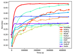
(a) LeNet & CIFAR-10

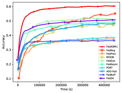
(b) CNN & CIFAR-10

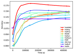
(c) ResNet & Tiny-ImageNet

Figure 3: The accuracy and training time for FedASMU and baseline approaches with CIFAR-10 and Tiny-ImageNet.

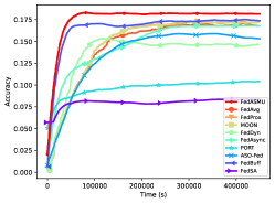
(a) LeNet & CIFAR-100

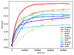
(b) CNN & CIFAR-100

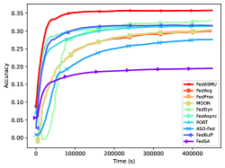
(c) ResNet & CIFAR-100

Figure 4: The accuracy and training time for FedASMU and baseline approaches with CIFAR-100.

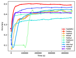
(a) AlexNet & CIFAR-10

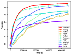
(b) VGG & CIFAR-10

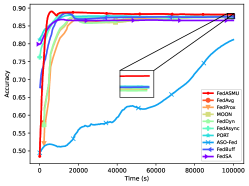
(c) TextCNN & IMDb

Figure 5: The accuracy and training time for FedASMU and baseline approaches with CIFAR-10 and IMDb

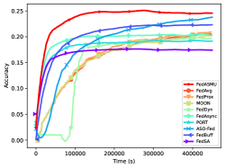
(a) AlexNet & CIFAR-100

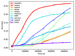
(b) VGG & CIFAR-100

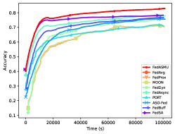
(c) LeNet & FMNIST

Figure 6: The accuracy and training time for FedASMU and baseline approaches with CIFAR-100 and FMNIST.

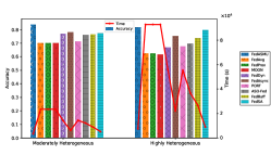
(a) Diversified device hetergeneity

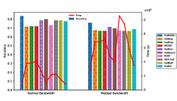
(b) Different network bandwidth

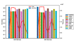
(c) Various numbers of devices

Figure 7: The accuracy and training time to achieve target accuracy (0.60) for FedASMU and baseline approaches with LeNet and FMNIST in diverse environments.

Hyper-parameter Fine-tuning

We conduct extra experiments on FMNIST and LeNet with varying trigger periods $\mathcal{T}$, $\eta_{\lambda^{i}}$, $\eta_{\sigma^{i}}$, and $\eta_{\iota^{i}}$, which correspond to little difference (0.0% to 0.8% with only one exceptional case of 2.4%) thanks to our dynamic model aggregation. Thus, FedASMU is not sensitive to the hyper-parameters and easy to fine-tune.

Comparison with Other Baselines

We carry out extra experimentation to compare FedASMU with three more recent works in asynchronous FL, i.e., FedDelay (Koloskova, Stich, and Jaggi 2022), SyncDrop (Dun et al. 2022), and AsyncPart (Wang, Zhang, and Wang 2021). We find FedASMU significantly outperforms these three approaches in terms of accuracy (0.063% for FedDelay, 11.2% for SyncDrop, and 6.7% for AsyncPart) and training time for a target accuracy (69.2% for FedDelay, 19.4% for SyncDrop, and 75.9% for AsyncPart).

Ablation Study for Request Time Slot Selection

We carry out extra experimentation with three heuristics. H1: the device sends the request just after the first local epoch. H2: the device sends the request in the middle of the local trainng. H3: the device sends the request at the last but one local epoch. The accuracy of our RL approach is significantly higher than H1 (2.4%), H2 (2.2%), and H3 (2.8%).

References

• Abad et al. (2020) Abad, M. S. H.; Ozfatura, E.; Gunduz, D.; and Ercetin, O. 2020. Hierarchical federated learning across heterogeneous cellular networks. In IEEE Int. Conf. on Acoustics, Speech and Signal Processing (ICASSP), 8866–8870.
• Acar et al. (2021) Acar, D. A. E.; Zhao, Y.; Matas, R.; Mattina, M.; Whatmough, P.; and Saligrama, V. 2021. Federated Learning Based on Dynamic Regularization. In Int. Conf. on Learning Representations (ICLR), 1–36.
• Bard (1998) Bard, J. F. 1998. Practical Bilevel Optimization: Algorithms and Applications. Springer.
• Bonawitz et al. (2019) Bonawitz, K.; Eichner, H.; Grieskamp, W.; Huba, D.; Ingerman, A.; Ivanov, V.; Kiddon, C.; Konevcnỳ, J.; Mazzocchi, S.; McMahan, B.; et al. 2019. Towards federated learning at scale: System design. Machine Learning and Systems (MLSys), 1: 374–388.
• Che et al. (2023a) Che, T.; Liu, J.; Zhou, Y.; Ren, J.; Zhou, J.; Sheng, V. S.; Dai, H.; and Dou, D. 2023a. Federated Learning of Large Language Models with Parameter-Efficient Prompt Tuning and Adaptive Optimization. In Conf. on Empirical Methods in Natural Language Processing (EMNLP). Singapore: Association for Computational Linguistics.
• Che et al. (2022) Che, T.; Zhang, Z.; Zhou, Y.; Zhao, X.; Liu, J.; Jiang, Z.; Yan, D.; Jin, R.; and Dou, D. 2022. Federated Fingerprint Learning with Heterogeneous Architectures. In IEEE Int. Conf. on Data Mining (ICDM), 31–40. IEEE.
• Che et al. (2023b) Che, T.; Zhou, Y.; Zhang, Z.; Lyu, L.; Liu, J.; Yan, D.; Dou, D.; and Huan, J. 2023b. Fast federated machine unlearning with nonlinear functional theory. In Int. Conf. on Machine Learning (ICML), 4241–4268. PMLR.
• Chen, Mao, and Ma (2021) Chen, M.; Mao, B.; and Ma, T. 2021. FedSA: A staleness-aware asynchronous Federated Learning algorithm with non-IID data. Future Generation Computer Systems (FGCS), 120: 1–12.
• Chen et al. (2021) Chen, S.; Xue, D.; Chuai, G.; Yang, Q.; and Liu, Q. 2021. FL-QSAR: a federated learning-based QSAR prototype for collaborative drug discovery. Bioinformatics, 36(22-23): 5492–5498.
• Chen et al. (2020) Chen, Y.; Ning, Y.; Slawski, M.; and Rangwala, H. 2020. Asynchronous online federated learning for edge devices with non-iid data. In IEEE Int. Conf. on Big Data (Big Data), 15–24.
• Dietterich (2000) Dietterich, T. G. 2000. Hierarchical reinforcement learning with the MAXQ value function decomposition. Journal of artificial intelligence research, 13: 227–303.
• Dun et al. (2022) Dun, C.; Garcia, M. H.; Jermaine, C.; Dimitriadis, D.; and Kyrillidis, A. 2022. Efficient and Light-Weight Federated Learning via Asynchronous Distributed Dropout. In Int. Conf. on Artificial Intelligence and Statistics (AISTATS).
• EU (2018) EU. 2018. European Union’s General Data Protection Regulation (GDPR). https://eugdpr.org/, accessed 2018-1.
• He et al. (2016) He, K.; Zhang, X.; Ren, S.; and Sun, J. 2016. Deep Residual Learning for Image Recognition. In IEEE Conf. on Computer Vision and Pattern Recognition (CVPR), 770–778. Las Vegas, USA: IEEE.
• Ho et al. (2013) Ho, Q.; Cipar, J.; Cui, H.; Lee, S.; Kim, J. K.; Gibbons, P. B.; Gibson, G. A.; Ganger, G.; and Xing, E. P. 2013. More effective distributed ml via a stale synchronous parallel parameter server. Advances in neural information processing systems (NeurIPS), 26.
• Horvath et al. (2021) Horvath, S.; Laskaridis, S.; Almeida, M.; Leontiadis, I.; Venieris, S.; and Lane, N. 2021. Fjord: Fair and accurate federated learning under heterogeneous targets with ordered dropout. Advances in Neural Information Processing Systems (NeurIPS), 34: 12876–12889.
• Hsu, Qi, and Brown (2019) Hsu, T.-M. H.; Qi, H.; and Brown, M. 2019. Measuring the effects of non-identical data distribution for federated visual classification. arXiv preprint arXiv:1909.06335.
• Jia et al. (2023) Jia, J.; Liu, J.; Zhou, C.; Tian, H.; Dong, M.; and Dou, D. 2023. Efficient Asynchronous Federated Learning with Sparsification and Quantization. Concurrency and Computation: Practice and Experience. To appear.
• Jiang et al. (2022) Jiang, Z.; Wang, W.; Li, B.; and Li, B. 2022. Pisces: Efficient Federated Learning via Guided Asynchronous Training. arXiv preprint arXiv:2206.09264.
• Jin et al. (2022) Jin, J.; Ren, J.; Zhou, Y.; Lv, L.; Liu, J.; and Dou, D. 2022. Accelerated Federated Learning with Decoupled Adaptive Optimization. In Int. Conf. on Machine Learning (ICML), volume 162, 10298–10322.
• Kairouz et al. (2021) Kairouz, P.; McMahan, H. B.; Brendan Avent, A. B.; Mehdi Bennis, A. N. B.; Bonawitz, K.; Charles, Z.; Cormode, G.; Cummings, R.; D’Oliveira, R. G.; Rouayheb, S. E.; Evans, D.; Gardner, J.; Garrett, Z.; Gascón, A.; Badih Ghazi, P. B. G.; Gruteser, M.; Harchaoui, Z.; He, C.; He, L.; Huo, Z.; Hutchinson, B.; Hsu, J.; Jaggi, M.; Javidi, T.; Joshi, G.; Khodak, M.; Konečný, J.; Korolova, A.; Koushanfar, F.; Koyejo, S.; Lepoint, T.; Liu, Y.; Mittal, P.; Mohri, M.; Nock, R.; Özgür, A.; Pagh, R.; Raykova, M.; Qi, H.; Ramage, D.; Raskar, R.; Song, D.; Song, W.; Stich, S. U.; Sun, Z.; Suresh, A. T.; Tramèr, F.; Vepakomma, P.; Wang, J.; Xiong, L.; Xu, Z.; Yang, Q.; Yu, F. X.; Yu, H.; and Zhao, S. 2021. Advances and Open Problems in Federated Learning. Foundations and Trends® in Machine Learning, 14(1).
• Karimireddy et al. (2020) Karimireddy, S. P.; Kale, S.; Mohri, M.; Reddi, S.; Stich, S.; and Suresh, A. T. 2020. SCAFFOLD: Stochastic Controlled Averaging for Federated Learning. In Int. Conf. on Machine Learning (ICML), volume 119, 5132–5143.
• Khodak, Balcan, and Talwalkar (2019) Khodak, M.; Balcan, M.-F. F.; and Talwalkar, A. S. 2019. Adaptive Gradient-Based Meta-Learning Methods. In Advances in Neural Information Processing Systems (NeurIPS), volume 32, 1–12.
• Koloskova, Stich, and Jaggi (2022) Koloskova, A.; Stich, S. U.; and Jaggi, M. 2022. Sharper Convergence Guarantees for Asynchronous SGD for Distributed and Federated Learning. ArXiv, abs/2206.08307.
• Krizhevsky, Hinton et al. (2009) Krizhevsky, A.; Hinton, G.; et al. 2009. Learning multiple layers of features from tiny images.
• Krizhevsky, Sutskever, and Hinton (2012) Krizhevsky, A.; Sutskever, I.; and Hinton, G. E. 2012. ImageNet Classification with Deep Convolutional Neural Networks. In Annual Conf. on Neural Information Processing Systems (NeurIPS), 1106–1114.
• Lai et al. (2021) Lai, F.; Zhu, X.; Madhyastha, H. V.; and Chowdhury, M. 2021. Oort: Efficient federated learning via guided participant selection. In USENIX Symposium on Operating Systems Design and Implementation (OSDI), 19–35.
• Le and Yang (2015) Le, Y.; and Yang, X. 2015. Tiny imagenet visual recognition challenge. CS 231N, 7(7): 3.
• LeCun et al. (1989) LeCun, Y.; Boser, B.; Denker, J.; Henderson, D.; Howard, R.; Hubbard, W.; and Jackel, L. 1989. Handwritten digit recognition with a back-propagation network. In Advances in Neural Information Processing Systems (NeurIPS), volume 2, 1–9.
• Li et al. (2022) Li, G.; Hu, Y.; Zhang, M.; Liu, J.; Yin, Q.; Peng, Y.; and Dou, D. 2022. FedHiSyn: A Hierarchical Synchronous Federated Learning Framework for Resource and Data Heterogeneity. In Int. Conf. on Parallel Processing (ICPP), 1–10. To appear.
• Li, Ota, and Dong (2018) Li, H.; Ota, K.; and Dong, M. 2018. Learning IoT in edge: Deep learning for the Internet of Things with edge computing. IEEE network, 32(1): 96–101.
• Li et al. (2014) Li, M.; Andersen, D. G.; Park, J. W.; Smola, A. J.; Ahmed, A.; Josifovski, V.; Long, J.; Shekita, E. J.; and Su, B.-Y. 2014. Scaling distributed machine learning with the parameter server. In USENIX Symposium on Operating Systems Design and Implementation (OSDI), 583–598.
• Li et al. (2021) Li, Q.; Diao, Y.; Chen, Q.; and He, B. 2021. Federated learning on non-iid data silos: An experimental study. arXiv preprint arXiv:2102.02079.
• Li, He, and Song (2021) Li, Q.; He, B.; and Song, D. 2021. Model-Contrastive Federated Learning. In IEEE/CVF Conf. on Computer Vision and Pattern Recognition (CVPR), 10713–10722.
• Li et al. (2020) Li, T.; Sahu, A. K.; Zaheer, M.; Sanjabi, M.; Talwalkar, A.; and Smith, V. 2020. Federated Optimization in Heterogeneous Networks. In Machine Learning and Systems (MLSys), volume 2, 429–450.
• Liu et al. (2022a) Liu, J.; Huang, J.; Zhou, Y.; Li, X.; Ji, S.; Xiong, H.; and Dou, D. 2022a. From distributed machine learning to federated learning: a survey. Knowledge and Information Systems (KAIS), 64(4): 885–917.
• Liu et al. (2022b) Liu, J.; Jia, J.; Ma, B.; Zhou, C.; Zhou, J.; Zhou, Y.; Dai, H.; and Dou, D. 2022b. Multi-Job Intelligent Scheduling With Cross-Device Federated Learning. IEEE Transactions on Parallel and Distributed Systems (TPDS), 34(2): 535–551.
• Liu et al. (2023a) Liu, J.; Wu, Z.; Yu, D.; Ma, Y.; Feng, D.; Zhang, M.; Wu, X.; Yao, X.; and Dou, D. 2023a. Heterps: Distributed deep learning with reinforcement learning based scheduling in heterogeneous environments. Future Generation Computer Systems (FGCS), 148: 106–117.
• Liu et al. (2023b) Liu, J.; Zhou, X.; Mo, L.; Ji, S.; Liao, Y.; Li, Z.; Gu, Q.; and Dou, D. 2023b. Distributed and deep vertical federated learning with big data. Concurrency and Computation: Practice and Experience, e7697.
• Liu et al. (2021) Liu, M.; Ho, S.; Wang, M.; Gao, L.; Jin, Y.; and Zhang, H. 2021. Federated learning meets natural language processing: A survey. arXiv preprint arXiv:2107.12603.
• Liu et al. (2020) Liu, Y.; Huang, A.; Luo, Y.; Huang, H.; Liu, Y.; Chen, Y.; Feng, L.; Chen, T.; Yu, H.; and Yang, Q. 2020. Fedvision: An online visual object detection platform powered by federated learning. In AAAI Conf. on Artificial Intelligence (AAAI), 13172–13179.
• Luo et al. (2021) Luo, M.; Chen, F.; Hu, D.; Zhang, Y.; Liang, J.; and Feng, J. 2021. No Fear of Heterogeneity: Classifier Calibration for Federated Learning with Non-IID Data. In Advances in Neural Information Processing Systems (NeurIPS), volume 34, 5972–5984.
• McMahan et al. (2017) McMahan, B.; Moore, E.; Ramage, D.; Hampson, S.; and y Arcas, B. A. 2017. Communication-efficient learning of deep networks from decentralized data. In Artificial Intelligence and Statistics (AISTATS), 1273–1282.
• Mitra et al. (2021) Mitra, A.; Jaafar, R.; Pappas, G. J.; and Hassani, H. 2021. Linear Convergence in Federated Learning: Tackling Client Heterogeneity and Sparse Gradients. In Advances in Neural Information Processing Systems (NeurIPS), volume 34, 14606–14619.
• Nguyen et al. (2022a) Nguyen, D. C.; Pham, Q.-V.; Pathirana, P. N.; Ding, M.; Seneviratne, A.; Lin, Z.; Dobre, O.; and Hwang, W.-J. 2022a. Federated learning for smart healthcare: A survey. ACM Computing Surveys (CSUR), 55(3): 1–37.
• Nguyen et al. (2022b) Nguyen, J.; Malik, K.; Zhan, H.; Yousefpour, A.; Rabbat, M.; Malek, M.; and Huba, D. 2022b. Federated Learning with Buffered Asynchronous Aggregation. In Int. Conf. on Artificial Intelligence and Statistics (AISTATS), volume 151, 3581–3607.
• Nishio and Yonetani (2019) Nishio, T.; and Yonetani, R. 2019. Client selection for federated learning with heterogeneous resources in mobile edge. In IEEE Int. Conf. on communications (ICC), 1–7.
• Ozkara et al. (2021) Ozkara, K.; Singh, N.; Data, D.; and Diggavi, S. 2021. QuPeD: Quantized Personalization via Distillation with Applications to Federated Learning. In Advances in Neural Information Processing Systems (NeurIPS), volume 34, 3622–3634.
• Park et al. (2021) Park, J.; Han, D.-J.; Choi, M.; and Moon, J. 2021. Sageflow: Robust federated learning against both stragglers and adversaries. In Advances in Neural Information Processing Systems (NeurIPS), volume 34, 840–851.
• Reddi et al. (2021) Reddi, S. J.; Charles, Z.; Zaheer, M.; Garrett, Z.; Rush, K.; Konevcný, J.; Kumar, S.; and McMahan, H. B. 2021. Adaptive Federated Optimization. In Int. Conf. on Learning Representations (ICLR), 1–38.
• Robbins and Monro (1951) Robbins, H.; and Monro, S. 1951. A stochastic approximation method. The annals of mathematical statistics, 400–407.
• Sattler, Müller, and Samek (2020) Sattler, F.; Müller, K.-R.; and Samek, W. 2020. Clustered federated learning: Model-agnostic distributed multitask optimization under privacy constraints. IEEE Transactions on Neural Networks and Learning Systems (TNNLS), 32(8): 3710–3722.
• Shi, Zhou, and Niu (2020) Shi, W.; Zhou, S.; and Niu, Z. 2020. Device scheduling with fast convergence for wireless federated learning. In IEEE Int. Conf. on Communications (ICC), 1–6.
• Shi et al. (2020) Shi, W.; Zhou, S.; Niu, Z.; Jiang, M.; and Geng, L. 2020. Joint device scheduling and resource allocation for latency constrained wireless federated learning. IEEE Transactions on Wireless Communications, 20(1): 453–467.
• Simonyan and Zisserman (2015) Simonyan, K.; and Zisserman, A. 2015. Very Deep Convolutional Networks for Large-Scale Image Recognition. In Int. Conf. on Learning Representations (ICLR).
• Smith et al. (2017) Smith, V.; Chiang, C.-K.; Sanjabi, M.; and Talwalkar, A. S. 2017. Federated Multi-Task Learning. In Advances in Neural Information Processing Systems (NeurIPS), volume 30, 1–11.
• Su and Li (2022) Su, N.; and Li, B. 2022. How Asynchronous can Federated Learning Be? In IEEE/ACM Int. Symposium on Quality of Service (IWQoS), 1–11.
• Sun et al. (2021) Sun, B.; Huo, H.; YANG, Y.; and Bai, B. 2021. PartialFed: Cross-Domain Personalized Federated Learning via Partial Initialization. In Advances in Neural Information Processing Systems (NeurIPS), volume 34, 23309–23320.
• Wang et al. (2020) Wang, J.; Liu, Q.; Liang, H.; Joshi, G.; and Poor, H. V. 2020. Tackling the Objective Inconsistency Problem in Heterogeneous Federated Optimization. In Advances in Neural Information Processing Systems (NeurIPS), volume 33, 7611–7623.
• Wang, Zhang, and Wang (2021) Wang, Z.; Zhang, Z.; and Wang, J. 2021. Asynchronous Federated Learning over Wireless Communication Networks. IEEE Int. Conf. on Communications (ICC), 1–7.
• Watkins and Dayan (1992) Watkins, C. J. C. H.; and Dayan, P. 1992. Technical Note Q-Learning. Machine Learning, 8: 279–292.
• Wu et al. (2020) Wu, W.; He, L.; Lin, W.; Mao, R.; Maple, C.; and Jarvis, S. 2020. SAFA: A semi-asynchronous protocol for fast federated learning with low overhead. IEEE Transactions on Computers, 70(5): 655–668.
• Xia and Zhao (2015) Xia, Z.; and Zhao, D. 2015. Online reinforcement learning by bayesian inference. In Int. Joint Conf. on Neural Networks (IJCNN), 1–6.
• Xiao, Rasul, and Vollgraf (2017) Xiao, H.; Rasul, K.; and Vollgraf, R. 2017. Fashion-mnist: a novel image dataset for benchmarking machine learning algorithms. arXiv preprint arXiv:1708.07747.
• Xie, Koyejo, and Gupta (2019) Xie, C.; Koyejo, S.; and Gupta, I. 2019. Asynchronous federated optimization. arXiv preprint arXiv:1903.03934.
• Xu et al. (2021) Xu, C.; Qu, Y.; Xiang, Y.; and Gao, L. 2021. Asynchronous federated learning on heterogeneous devices: A survey. arXiv preprint arXiv:2109.04269.
• Yang et al. (2021) Yang, C.; Wang, Q.; Xu, M.; Chen, Z.; Bian, K.; Liu, Y.; and Liu, X. 2021. Characterizing impacts of heterogeneity in federated learning upon large-scale smartphone data. In Web Conf. (WWW), 935–946.
• Zhang et al. (2022) Zhang, H.; Liu, J.; Jia, J.; Zhou, Y.; and Dai, H. 2022. FedDUAP: Federated Learning with Dynamic Update and Adaptive Pruning Using Shared Data on the Server. In Int. Joint Conf. on Artificial Intelligence (IJCAI), 2776–2782.
• Zhou et al. (2022) Zhou, C.; Liu, J.; Jia, J.; Zhou, J.; Zhou, Y.; Dai, H.; and Dou, D. 2022. Efficient device scheduling with multi-job federated learning. In AAAI Conf. on Artificial Intelligence (AAAI), 9971–9979.
• Zhou et al. (2021a) Zhou, C.; Tian, H.; Zhang, H.; Zhang, J.; Dong, M.; and Jia, J. 2021a. TEA-fed: time-efficient asynchronous federated learning for edge computing. In ACM Int. Conf. on Computing Frontiers, 30–37.
• Zhou et al. (2021b) Zhou, Y.; Pu, G.; Ma, X.; Li, X.; and Wu, D. 2021b. Distilled One-Shot Federated Learning. arXiv preprint arXiv:2009.07999, abs/2009.07999(1): 1–16.
• Zinkevich et al. (2010) Zinkevich, M.; Weimer, M.; Smola, A. J.; and Li, L. 2010. Parallelized Stochastic Gradient Descent. In Advances in Neural Information Processing Systems (NeurIPS), volume 23, 1–37.
• Zoph and Le (2017) Zoph, B.; and Le, Q. V. 2017. Neural Architecture Search with Reinforcement Learning. In Int. Conf. on Learning Representations (ICLR).