Cosmological FLRW phase transitions and micro-structure under Kaniadakis statistics

Abstract

This article is devoted to the study of the thermodynamics phase transitions and critical phenomena of an FLRW cosmological model under the so-called Kaniadakis’s statistics. The equation of state is derived from the corrected Friedmann field equations and the thermodynamics unified first law. This reveals the existence of non-trivial critical points where a first-order phase transition takes place. The system behaves as an “inverted” van der Waals fluid in this concern. Interestingly, the numerical values of the critical exponents are the same as those of the van der Waals system. Besides, to obtain more insights into the thermodynamics description, the so-called Ruppeiner’s geometry is studied through the normalized scalar curvature, disclosing this invariant zone where the system undergoes repulsive/attractive interactions. Near the critical point, this curvature provides again the same critical exponent and universal constant value as for van der Waals fluid.

I Introduction

The so-called Kaniadakis’s entropy Kaniadakis:2002zz ; Kaniadakis:2005zk , has attracted much interest in recent years. This information measure corresponds to a relativistic generalization of the classical and well-known Boltzmann-Gibbs-Shannon entropy. In Moradpour:2020dfm , using the relation between Tsallis’s and Kaniadakis’s entropies, it was possible to extrapolate this latter into the gravitational context. Specifically, re-written it in terms of the black hole (BH) entropy Bekenstein:1973ur . This achievement allowed to explore a series of gravitational phenomena such as observational constraints on holographic dark energy Hernandez-Almada:2021aiw ; Hernandez-Almada:2021rjs ; Drepanou:2021jiv ; Nojiri:2022dkr ; Nojiri:2022aof ; Odintsov:2023vpj ; Sania:2023fjx , generalized second and third laws of thermodynamics Abreu:2021kwu ; Moradpour:2021soz , slow-roll inflation Lambiase:2023ryq , BHs thermodynamics Luciano:2023bai ; Odintsov:2023qfj ; Cimidiker:2023kle ; Lymperis:2021qty , micro-canonical and canonical descriptions Nojiri:2023ikl , generalized entropy and its microscopic interpretation Odintsov:2022qnn ; Nojiri:2023bom and general cosmological setups Lymperis:2021qty ; Sheykhi:2023aqa , to name a few.

In this respect, it is worth noticing that most of the mentioned investigations were possible due to the so-called gravity-thermodynamics conjecture Jacobson:1995ab ; Padmanabhan:2003gd ; Padmanabhan:2002sha . This is so because, starting from a purely thermodynamics description, this conjecture allows us to determine the field equations Lymperis:2021qty ; Sheykhi:2023aqa . Of course, in doing so, some assumptions and prescriptions are necessary. For instance, for spherically symmetric space-times, one needs to consider that the Misner-Sharp energy Misner:1964je obeys the classical thermodynamics relation, that is, it is equal to the product of the density of the matter distribution by the thermodynamics volume. Also, it is necessary to consider that Clausius’s relation holds. Etc.

From the side of static/stationary space-times, for example, BHs, the thermodynamics studies were performed by using the approach given in the seminal articles Smarr:1972kt ; Bardeen:1973gs ; Hawking:1975vcx ; Gibbons:1976ue by replacing the Bekenstein’s entropy Bekenstein:1973ur by the Kaniadakis entropy Kaniadakis:2002zz ; Kaniadakis:2005zk ; Moradpour:2020dfm . On the other hand, for cosmological models, being these space-times dynamical, the above scheme was done by using the thermodynamics unified first law (UFL) Hayward:1993wb ; Hayward:1994bu ; Hayward:1997jp , and of course, changing the event horizon (EH) by the apparent horizon (AH) Kodama:1979vn ; Faraoni:2011hf ; Faraoni:2015ula .

So, taking advantage of these antecedents, a natural question arises: Can the usual gravitational entropy (Bekenstein’s entropy) be replaced with Kaniadakis’s entropy to get non-trivial thermodynamics phenomena for an FLRW cosmological model? In case of positive answer, are these phenomena feasible at least from a pure theoretical point of view? These simple questions arise because in the General Relativity (GR) scenario, it is well-known that the FLRW model does not present thermodynamics phase transitions Abdusattar:2023pck . Nevertheless, this situation drastically changes if one introduces further degrees of freedom, such as scalar fields, other than the gravitational ones Fernandes:2021dsb . Indeed, any additional field minimally or not minimally coupled to gravity shall modify the field equations and all the thermodynamics-associated quantities, such as the entropy, Misner-Sharp energy, etc. Therefore, one expects (in principle) a more involved description of thermodynamics.

It is clear from the above paragraph that once a modified theory of gravity and its equations are fully provided, and one is able from the Euclidean path integral formulation to obtain the full thermodynamics description. Here, the situation is quite different because assuming that the UFL “always” holds and taking from the very beginning a specific form of the entropy, the equations of motion are coming. So, in principle, nothing prevents us from using this fact as the starting point to investigate under what conditions intriguing thermodynamics phenomena are happening.

So, utilizing the above fact, the main aim and motivation of the present research is to realize how Kaniadakis’s information measure modifies the thermodynamic behavior of an FLRW cosmological model. To achieve this goal, we use the corrected Friedmann field equations at leading order in the parameter $K$ Sheykhi:2023aqa , determining in this way the equation of state and its critical points in an analytical way. The system undergoes a first-order phase transition, similar to the transition of a van der Waals’s fluid, but in the “opposite direction”. By this, we mean that the stable/unstable regions in van der Waals fluid are permuted by unstable/stable zones in the present system. Despite this strange feature, the critical exponents’ numerical values coincide with those found for a van der Waals fluid (in the mean field approximation). Moreover, to obtain further insights into the micro-structure of the system, we perform the analysis from the point of view of the so-called Ruppiner’s geometry Ruppeiner:1981znl ; Ruppeiner:1983zz ; Ruppeiner:1995zz . This analysis reveals the regions where attractive/repulsive interactions dominate. Interestingly, near the critical point, the normalized scalar curvature also has the critical exponent value obtained in mean field theory.

The article is organized as follows: Sect. II briefly reviews Kaniadakis’s entropy formulation in the gravitational context, modified Friedmann field equations, the equation of state obtained from the UFL, and the corrected Misner-Sharp energy expression in Sect. III, the thermodynamics phase transition, critical exponents, and Ruppeiner’s geometry are analyzed in detail—finally, Sect. IV concludes the present research.

The mostly positive signature $(-,+,+,+)$ is used throughout the article.

II Modified Friedmann equations

In this section, we review in short how the Friedmann field equations are modified when the well-known Kaniadakis entropy (also known as the $K$-Entropy)Kaniadakis:2002zz ; Kaniadakis:2005zk is employed. These expressions are obtained through the UFL on an FLRW metric. Moreover, the corresponding expression for the corrected Misner-Sharp (MS) energy Misner:1964je and the equation of state-driven thermodynamics description of the FLRW Universe within this modified scenario are given.

II.1 FLRW model and Kaniadakis information measure

The original Kaniadakis entropy expression is given by Kaniadakis:2002zz ; Kaniadakis:2005zk

$$S_{K}=-k_{B}\sum_{i}n_{i}\text{ln}_{(K)}n_{i}\quad\mbox{with}\quad ln_{(K)}x=\frac{x^{K}-x^{-K}}{2K},$$ (1)

or equivalently Abreu:2016avj ; Abreu:2017fhw ; Abreu:2017hiy ; Abreu:2018mti

$$S_{K}=-k_{B}\sum_{i=1}^{\mathcal{W}}\frac{P_{i}^{1+K}-P_{i}^{1-K}}{2K},$$ (2)

with $P_{i}$ the probability of a system being in a specific microstate and $\mathcal{W}$ the total configuration number. Clearly, this information measure is a generalization of the seminal Boltzmann-Gibbs-Shannon entropy. In a more widely context, in the gravitational framework, it has been shown that the Kaniadakis entropy (1) can be written as follows Moradpour:2020dfm

$$S_{K}=\frac{1}{K}\text{sinh}{\left(KS_{\text{BH}}\right)},$$ (3)

being $S_{\text{BH}}$ the BH entropy given by Bekenstein:1973ur

$$S_{\text{BH}}=\frac{A}{4}.$$ (4)

It is worth mentioning that the area $A$ appearing in the above expression corresponds to the area of the event horizon BH; however, as we are most interested in studying cosmological models, this area should be replaced by the area of the apparent horizon (AH). So, the Eq. (3) shall be expressed as

$$S_{K}=\frac{1}{K}\text{sinh}{\left(KS_{\text{AH}}\right)},\quad S_{\text{AH}}=\frac{A_{\text{AH}}}{4},\quad 0<K<1.$$ (5)

This result is universal in RG; the entropy is always a quarter of the area, independently of the model at hand. This is so because this expression is derived from the Euclidean action using the on-shell Lagrangian of the theory, a fundamental object of the theory.

In this case, since there is no associated action principle from which the Kaniadakis entropy can be derived, one option to find the modified Friedmann field equations is to appeal to the gravitational-thermodynamics conjecture Jacobson:1995ab ; Padmanabhan:2003gd ; Padmanabhan:2002sha . Given a thermodynamic law with corresponding identifications and interpretations of gravitational quantities, the field equations and their corrections can be consistently found. As the FLRW

$$ds^{2}=-dt^{2}+a^{2}(t)\left(\frac{dr^{2}}{1-kr^{2}}+r^{2}d\Omega^{2}\right)$$ (6)

model is a dynamical system, the associated thermodynamics law to describe it properly, is the so-called UFL Hayward:1993wb ; Hayward:1994bu ; Hayward:1997jp

$$\nabla_{i}E=A\psi_{i}+W\nabla_{i}V,$$ (7)

where the energy–supply is encoded by the vector $A\psi_{i}$ and the density work by $W$. In general, these last two objects are defined by

$$\psi_{i}\equiv T^{j}_{i}\nabla_{i}R+W\nabla_{i}R,$$ (8)

and

$$W\equiv-\frac{1}{2}h_{ij}T^{ij},$$ (9)

respectively. Nevertheless, as the thermodynamics takes place on the AH, to determine this surface, the line element (6) can be cast as a warped product between a two-dimensional manifold $\mathcal{M}_{2}$ (the $t-r$ plane) and a two-sphere $\mathbb{S}^{2}$ as

$$ds^{2}=h_{ij}dx^{i}dx^{j}+R^{2}d\Omega^{2},$$ (10)

where $h_{ij}$ is the induced metric on the manifold $\mathcal{M}_{2}$ and $R(t,r)\equiv a(t)r$ is the physical radius. So, it is not hard to show that the AH is the solution of the following differential equation

$$h^{ij}\nabla_{i}R\nabla_{j}R=0\Rightarrow R_{\text{AH}}=\frac{1}{\sqrt{H^{2}+\frac{k}{a^{2}}}}.$$ (11)

Notice that Latin indexes run over $i,j=t,r$. In this way, the trace of the energy-momentum tensor $h_{ij}T^{ij}$ on the t-r orthogonal to the two-spheres of symmetry is given by $h_{ij}T^{ij}=p-\rho$, being $p$ the isotropic pressure and $\rho$ the density of the perfect fluid filling the Universe.

Now, projecting the UFL (7) along the AH, one obtains (Hayward:1997jp, )

$$z^{i}\nabla_{i}E=\frac{\kappa_{\text{HK}}}{8\pi}z^{i}\nabla_{i}A+Wz^{i}\nabla_{i}V,$$ (12)

where the following identification has been done $A\psi_{i}=\frac{\kappa_{\text{HK}}}{8\pi}z^{i}\nabla_{i}A$ (Hayward:1997jp, ; Cai:2006rs, ) and $z^{i}$ is a vector tangent to the AH. This step allows us to identify the so-called Hayward-Kodama (HK) surface gravity $\kappa_{\text{HK}}$. Taking into account that it is a purely geometric object (independent of the underlying theory), it has the following definition (Hayward:1997jp, )

$$\kappa_{\text{HK}}=\frac{1}{2\sqrt{-h}}\partial_{i}\left(\sqrt{-h}h^{ij}\partial_{j}R\right),$$ (13)

where $h\equiv\text{det}(h_{ij})$. Therefore, the temperature $T$ is defined as

$$T=\frac{\kappa_{\text{HK}}}{2\pi}.$$ (14)

Despite having the same definition as Hawking’s temperature Hawking:1975vcx , the main difference is that the HK surface gravity is a dynamical object.

After replacing the surface gravity with the temperature in the project UFL (12), the first term on the right-hand side can be recognized as the Clausius relation, $dE=-TdS$, where by using (5) and some algebraic reduction, one arrives to Lymperis:2021qty

$$\text{cosh}{\left[\frac{K\pi}{H^{2}+\frac{k}{a^{2}}}\right]}\left[\dot{H}-\frac{k}{a^{2}}\right]=-4\pi G(\rho+p),$$ (15)

$$\text{cosh}{\left[\frac{K\pi}{H^{2}+\frac{k}{a^{2}}}\right]}\left[H^{2}+\frac{k}{a^{2}}\right]-K\pi\text{shi}{\left[\frac{K\pi}{H^{2}+\frac{k}{a^{2}}}\right]}=\frac{8\pi G}{3}\rho,$$ (16)

where $\operatorname{shi}(x)\equiv\int_{0}^{x}\sinh\left(x^{\prime}\right)/x^{\prime}dx^{\prime}$. It should noted that in deriving the above expressions, it was assumed the energy MS $E=\rho V$, with $V=4\pi R^{3}_{\text{AH}}/3$. Obviously, taking the limit $K\rightarrow 0$ the Eqs. (15)-(16) become the original GR Friedmann field equations. Furthermore, these expressions can be formally expressed in terms of the AH and its variation through (11).

II.2 The equation of state and the Misner-Sharp energy

At this stage, we can derive the equation of state (EoS) of the cosmological FLRW model. To achieve this goal, from the Eqs. of motion (15)-(16) the density work (9) reads

$$\begin{split}W=\frac{T}{2R_{\text{AH}}}\text{cosh}{(K\pi R^{2}_{\text{AH}})}+\frac{1}{8\pi R^{2}_{\text{AH}}}\text{cosh}{(K\pi R^{2}_{\text{AH}})}&\\ -\frac{3K}{8}\text{shi}{(K\pi R^{2}_{\text{AH}})},\end{split}$$ (17)

where

$$T=-\frac{1}{2\pi R_{\text{AH}}}\left(1-\frac{\dot{R}_{\text{AH}}}{2HR_{\text{AH}}}\right)$$ (18)

has been used. Now, as $W=P$, being $P$ the pressure of the whole system, the Eq. (17) provides

$$\begin{split}P(v,T)=\frac{T}{v}\text{cosh}{\left(\frac{K\pi v^{2}}{4}\right)}+\frac{1}{2\pi v^{2}}\text{cosh}{\left(\frac{K\pi v^{2}}{4}\right)}&\\ -\frac{3K}{8}\text{shi}{\left(\frac{K\pi v^{2}}{4}\right)},\end{split}$$ (19)

where we have introduced the molar volume $v=2R_{\text{AH}}$. As can be seen from the EoS (19), it is not possible to obtain the information about the critical points $\{v_{c},T_{c}\}$, where possible phase transitions are happening, in an analytical way. Of course, solving the system numerically will be interesting, including all the information to check under what conditions phase transitions are occurring. Nevertheless, it is interesting to see how the first corrections influence the thermodynamics description of these modified Friedmann field equations. So, expanding the EoS (19) around $K=0$ and keeping just the leading order, one gets

$$\begin{split}P(v,T)=\frac{T}{v}+\frac{1}{2\pi v^{2}}+\left(\frac{\pi^{2}}{32}v^{3}T-\frac{5\pi}{64}v^{2}\right)K^{2}+\mathcal{O}\left(K^{4}\right).\end{split}$$ (20)

Next, the criticality conditions for the EoS (20) are

$$\left(\frac{\partial P}{\partial v}\right)\bigg{|}_{T}=\left(\frac{\partial^{2}P}{\partial v^{2}}\right)\bigg{|}_{T}=0.$$ (21)

These conditions lead to

$$\begin{split}v_{c}=\frac{2}{\sqrt{\pi}}\left(\frac{1}{K^{2}}\right)^{1/4}\left(\frac{8-2\sqrt{15}}{\sqrt{15}}\right)^{1/4},&\\ \quad T_{c}=-\sqrt{\frac{5K}{12\pi}}\left(\frac{8+2\sqrt{15}}{\sqrt{15}}\right)^{-1/4}.\end{split}$$ (22)

Interestingly, the resulting critical temperature $T_{c}$, at which the phase transition occurs, is negative. In this case, the above result can be justified as follows:

1. For those cosmological models presenting an expanding evolution ($\dot{R}_{\text{AH}}>0$), the matter distribution filling the Universe could be, for example (from a purely theoretical point of view) the so-called stiff matter, that is, a matter field satisfying the barotropic EoS $p=\rho$. This type of matter content was used to study the early Universe stage, leading to a classical bouncing model free from singularities Oliveira-Neto:2011uhf ; Banks:2008ep . What is more, the same issue was tackled from the quantum point of view in Falciano:2007yf .

   Usually, in this scenario, this kind of matter distribution is accompanied by a negative temperature Vieira:2016lyj . Therefore, a cosmological model with a negative temperature is feasible. On the other hand, the final sign of the temperature strongly depends on the sign of the surface gravity and the causal feature of the AH Binetruy:2014ela ; Helou:2015yqa ; Helou:2015zma . In this concern, an expanding cosmology has a past AH leading to $T\propto-\kappa_{\text{HK}}$, while a stiff matter content leads to an outer AH, providing $\kappa_{\text{HK}}>0$, so $T<0$.

2. Another scenario where a negative temperature drives the cosmological evolution is the case of contracting cosmology ($\dot{R}_{\text{AH}}<0$). In such a case, the matter distribution corresponds to a phantom field Cruz:2023wtq , satisfying $p=\omega\rho$ with $\omega<-1$. The main difference with respect to the stiff matter case is that the causal structure of the AH here corresponds to an inner-future horizon. The inner characteristic means $\kappa_{\text{HK}}<0$, whilst the future feature implies $T\propto+\kappa_{\text{HK}}$, thus $T<0$. Nevertheless, this possibility is discarded for the present case since the system (21) has a not real or positive defined volume.

The previous discussion determines that the present model is dominated by a stiff matter distribution with a negative temperature, corresponding to an expanding cosmological era characterized by an outer-past AH.

After replacing the critical points (22) into the EoS (20), one gets the following values for the critical pressure $P_{c}$

$$P(v_{c},T_{c})=P_{c}=-\frac{\sqrt{75+40\sqrt{15}}}{12\sqrt{2}}K.$$ (23)

Next, the study of phase transitions is better carried out by expression of the EoS (20) as a function of the reduced variables

$$\tilde{P}\equiv\frac{P}{P_{c}},\quad\tilde{v}\equiv\frac{v}{v_{c}},\quad\tilde{T}\equiv\frac{T}{T_{c}},$$ (24)

leading to

$$\begin{split}\tilde{P}=\frac{1}{2\left(6\sqrt{5}-5\sqrt{3}\right)\tilde{v}^{2}}\bigg{(}-3\sqrt{3}+6\sqrt{5}\tilde{v}\tilde{T}+3\bigg{(}4\sqrt{5}&\\ -5\sqrt{3}\bigg{)}\tilde{v}^{4}+\left(8\sqrt{3}-6\sqrt{5}\right)\tilde{v}^{5}\tilde{T}\bigg{)}.\end{split}$$ (25)

As can be seen, the reduced EoS (25) is independent of the parameter $K$. However, the critical values are depending on the parameter $K$.

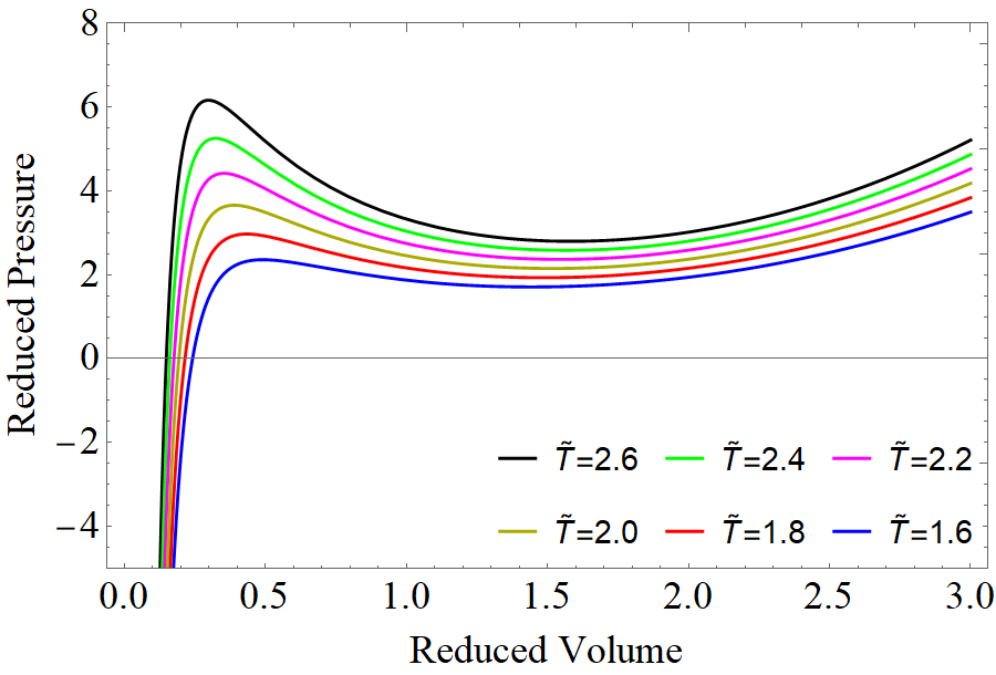
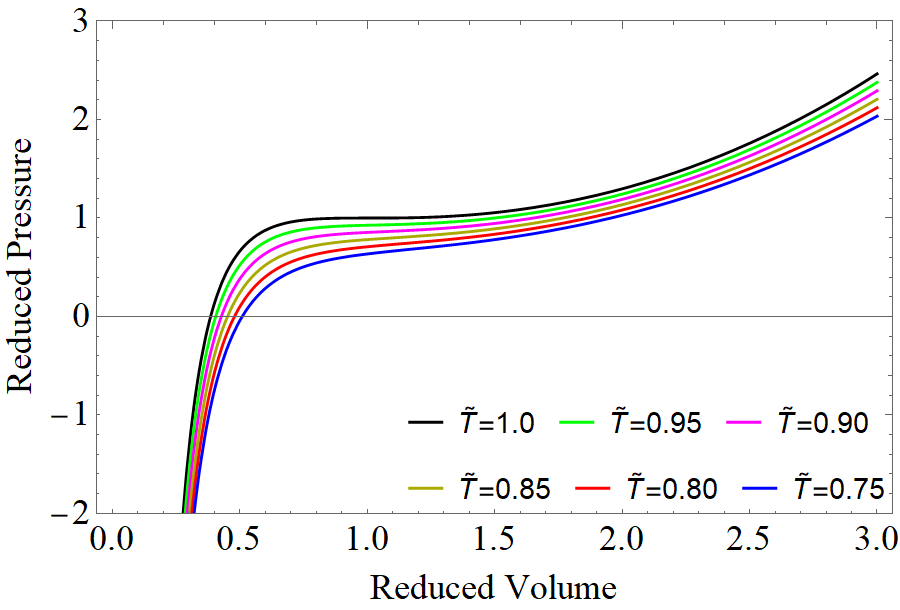
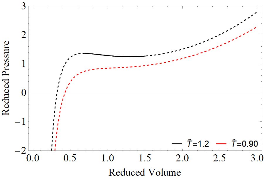
Figure 1: Left panel: The reduced pressure versus the reduced volume for different values of temperature above the critical one. It is clear that the system undergoes a phase transition. Middle panel: The trend of the reduced pressure versus the reduced volume for different values of temperature below the critical one. Here, the system does not present any abrupt behavior, and there is no phase transition. Right panel: A comparison between two isotherms, one for $\tilde{T}>0$ (black line) and the second one for $\tilde{T}<0$ (red line). A finite stable region (solid black line) occurs when the system undergoes a phase transition. In contrast, when no phase transition is happening, the system is completely unstable from the thermodynamic point of view.

Finally, to close this section, we are going to provide the corrected MS energy. To achieve this aim, one can proceed in two equivalent ways, that is, i) using $E=\rho V$ or ii) by integrating the UFL (7). First, this relation is valid since we are dealing with a spherical system, where the volume of the reservoir coincides, in this case, with the physical volume $V$ (the thermodynamic volume). Of course, this assumption was considered in deriving the corrected Friedmann field equations Lymperis:2021qty ; Sheykhi:2023aqa from the UFL (7). In the second case, the UFL can be expressed as

$$dE=-TdS+WdV\Rightarrow E=\int(-TdS+WdV).$$ (26)

The former provides

$$E=\frac{R_{\text{AH}}}{2}\text{cosh}{\left(K\pi R^{2}_{\text{AH}}\right)}-\frac{\pi K}{2}R^{3}_{\text{AH}}\text{shi}{\left(K\pi R^{2}_{\text{AH}}\right)}.$$ (27)

Expanding around $K$, the above expression provides

$$E=\frac{R_{\text{AH}}}{2}-\frac{\pi^{2}R^{5}_{\text{AH}}}{4}K^{2}+\mathcal{O}(K^{4}),$$ (28)

this result also can be obtained from (26) inserting the expanded expression of (5) and performing the algebraic steps. In the limit $K\rightarrow 0$, the expression (26) reduces to MS energy corresponding to an entropy $S=A_{\text{AH}}/4$.

III Thermodynamics description

This section is devoted to the analysis of the thermodynamics phase transitions and critical points. The phase transition study is performed by employing different perspectives. One using the usual thermodynamics tools Goldenfeld:1992qy , that is, by checking the EoS and associated thermodynamics quantities behavior and the second one from the point of view of the so-called Ruppeiner’s geometry Ruppeiner:1981znl ; Ruppeiner:1983zz ; Ruppeiner:1995zz ; Ruppeiner:2013yca ; Ruppeiner:2018pgn ; Ruppeiner:2023wkq . This latter shall provide us some insights not only about phase transitions (through the Ruppeiner’s scalar curvature), also some information about how the particles of the fluid interact ı.e., an idea about the micro-structure of the system.

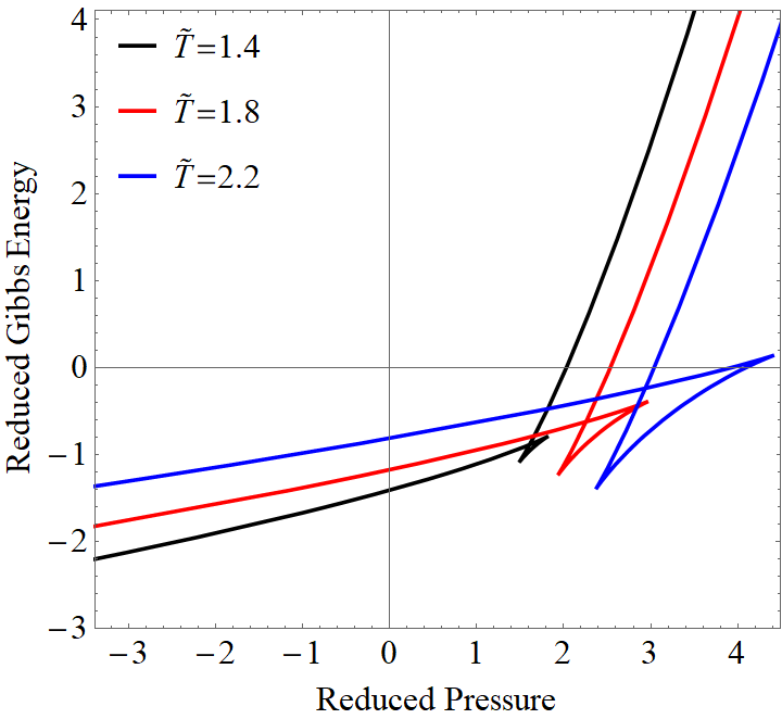
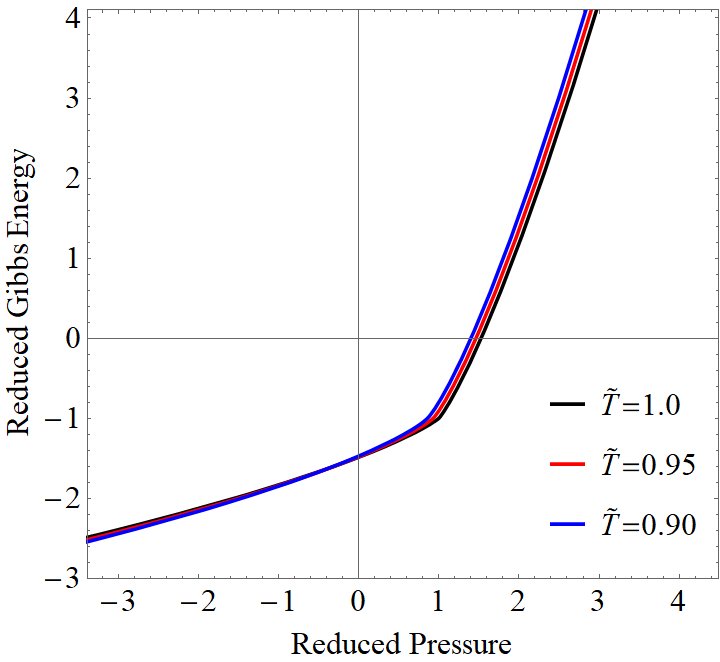
Figure 2: Left panel: The trend of the reduced Gibbs’s free energy versus the reduced pressure, for $\tilde{T}>T_{c}$. As can be appreciated, this thermodynamics quantity exhibits the classical swallowtail shape, corresponding to a first-order phase transition. Right panel: The behavior of the reduced Gibbs’s free energy against the reduced pressure, for $\tilde{T}<T_{c}$. In this case, this thermodynamics response function is smooth; no phase transition is occurring.

III.1 Phase transitions

The EoS (25) behavior is depicted in Fig. 1 (isotherms). The left panel shows the trend of the isotherms for temperatures above the critical one, and the middle panel displays the behavior for values below the critical point. In comparison with a real gas (van der Waals’s gas), for example, the behavior of the EoS (25) illustrated in Fig. 1 is quite different. First of all, the phase transition occurs above the critical point (left panel), while below it, the system does not present any drastic change (middle panel). Moreover, for those values below the critical point, the system is completely unstable, that is, $\partial\tilde{P}/\partial\tilde{v}>0$. On the other hand, for values above the critical temperature, there is a “small” region where the system is stable   i.e., $\partial\tilde{P}/\partial\tilde{v}<0$. These regions are clear from the right panel in Fig. 1, where the dashed red line shows the isotherm for $\tilde{T}=0.90$, being explicit the increasing behavior of $\tilde{P}$ with increasing volume $\tilde{v}$. The black dashed portions are displaying the zones where the system is unstable for values above the critical value, $\tilde{T}=1.2$, while the solid region on this curve shows the stable portion.

Again, comparing the present case with the canonical van der Waals’s scenario, stable branches are larger than the present system in the latter, and unstable states are bounded. Here, the situation is quite unconventional because the phase transition region seems to be stable. To account for the existence of first-order phase transition, Fig. 2 shows the behavior of the reduced Gibbs’s free energy versus the reduced pressure

$$\begin{split}\tilde{G}(\tilde{v},\tilde{T})=\frac{1}{12\left(2\sqrt{15}-5\right)\tilde{v}}\bigg{[}-36+4\left(4\sqrt{15}-15\right)\tilde{v}^{4}&\\ -9\left(\sqrt{15}-4\right)\tilde{v}^{5}\tilde{T}-12\tilde{v}\tilde{T}\text{Log}(\tilde{v})\bigg{]}.\end{split}$$ (29)

The left panel illustrates the behavior for values $\tilde{T}>T_{c}$, exhibiting the characteristic swallowtail shape. On the other hand, the right panel of Fig. 2 displays the trend for values $\tilde{T}<T_{c}$, where the reduced Gibbs’s free energy is completely smooth.

III.2 Critical exponents

Compute the values of the critical exponent associated with this system to get more insights into the critical point. To do so, one needs to compute the behavior of the heat capacity at constant volume $C_{v}$, the shear viscosity $\eta$, the compressibility $\kappa_{T}$ and pressure $P$ following

$$C_{v}\sim|\tau|^{-\hat{\alpha}},$$ (30)

$$\eta\sim v_{l}-v_{s}\sim|\tau|^{\hat{\beta}},$$

$$\kappa_{T}=-\frac{1}{v}\left(\frac{\partial v}{\partial P}\right)\bigg{|}_{T}\sim|\tau|^{-\hat{\gamma}},$$

$$P-P_{c}\sim\left|v-v_{c}\right|^{\hat{\delta}},$$

with $\{\hat{\alpha},\hat{\beta},\hat{\gamma},\hat{\delta}\}$ the critical exponents. To obtain the values of these quantities, it is necessary to expand the pressure (20) around the critical values $\{v_{c},T_{c}\}$. This expansion produces

$$\begin{split}P=P_{c}+\left[\left(\frac{\partial P}{\partial T}\right)\bigg{|}_{v}\right]\bigg{|}_{c}\left(T+T_{c}\right)+\frac{1}{2!}\left[\left(\frac{\partial^{2}P}{\partial T^{2}}\right)\bigg{|}_{v}\right]\bigg{|}_{c}&\\ \times\left(T+T_{c}\right)^{2}+\left[\left(\frac{\partial^{2}P}{\partial T\partial v}\right)\right]\bigg{|}_{c}\left(T+T_{c}\right)\left(v-v_{c}\right)&\\ +\frac{1}{3!}\left[\left(\frac{\partial^{3}P}{\partial v^{3}}\right)\bigg{|}_{T}\right]\bigg{|}_{c}\left(v-v_{c}\right)^{3}+\ldots\end{split}$$ (31)

Notice that the criticality conditions (21) have been used in the above expansion. Also, those terms corresponding to the expansion around the critical temperature are proportional to $(T+T_{c})$ and not to $(T-T_{c})$ since our thermodynamics system has a negative absolute temperature. Now, introducing the dimensionless variables $\tau\equiv T/T_{c}+1$ and $\omega\equiv v/v_{c}-1$ and the reduced variables, the expression (31) reads

$$\tilde{P}=1+A\tau+B\tau\omega+C\tau\omega^{2}+D\omega^{3}+\ldots,$$ (32)

where the coefficients $\{A,B,C,D\}$ are given by

$$A =-\frac{4}{35}(5+2\sqrt{15}), B =-\frac{4}{35}(15-\sqrt{15})$$ (33)

$$C =2\sqrt{\frac{3}{5}}, D =\frac{2}{7}(1-\sqrt{15}).$$

As the reduced pressure (25) is linear in $\tilde{T}$, the heat capacity at constant volume $C_{v}$ is zero, implying $\hat{\alpha}=0$. Now, employing Maxwell’s area rule (to determine the remaining critical exponents)

$$\tilde{P}^{*}\left(\omega_{s}-\omega_{l}\right)=\int^{\omega_{s}}_{\omega_{l}}\tilde{P}d\omega,$$ (34)

from (32) one obtains

$$\begin{split}\tilde{P}^{*}\left(\omega_{s}-\omega_{l}\right)=\int^{\omega_{l}}_{\omega_{s}}\left(1+A\tau+B\tau\omega+C\tau\omega^{2}+D\omega^{3}\right)d\omega.\end{split}$$ (35)

In the above integral expression, $\omega_{s}$ and $\omega_{l}$ stand for the so-called small and large volumes in two different phases. In between these two, we have a mixture of both of them. Next, the vapor’s endpoint and the liquid’s starting point have the same pressure. Similarly, here the pressure does not change, that is, $\tilde{P}^{*}=\tilde{P}_{l}=\tilde{P}_{s}$. Therefore, from (32) one gets

$$B\tau\left(\omega_{l}-\omega_{s}\right)+C\tau\left(\omega^{2}_{l}-\omega^{2}_{s}\right)+D\left(\omega^{3}_{l}-\omega^{3}_{s}\right)=0.$$ (36)

On the other hand, the integral in the right member of (35) provides

$$\begin{split}\left(1+A\tau\right)\left(\omega_{l}-\omega_{s}\right)+\frac{B\tau}{2}\left(\omega^{2}_{l}-\omega^{2}_{s}\right)+\frac{C\tau}{3}\left(\omega^{3}_{l}-\omega^{3}_{s}\right)&\\ +\frac{3D}{4}\left(\omega^{4}_{l}-\omega^{4}_{s}\right)=\tilde{P}(\omega_{s},\tau)\left(\omega_{s}-\omega_{l}\right).\end{split}$$ (37)

Solving the set of Eqs. (36)-(37) for $\omega_{s}$ and $\omega_{l}$, one obtains the following result

$$\tilde{v}_{s} =1+\sqrt{\hat{A}_{s}\tau+\hat{B}_{s}\tau^{2}}+\hat{C}_{s}\tau,$$ (38)

$$\tilde{v}_{l} =1+\sqrt{\hat{A}_{l}\tau+\hat{B}_{l}\tau^{2}}+\hat{C}_{l}\tau,$$

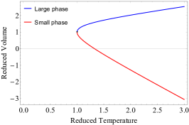
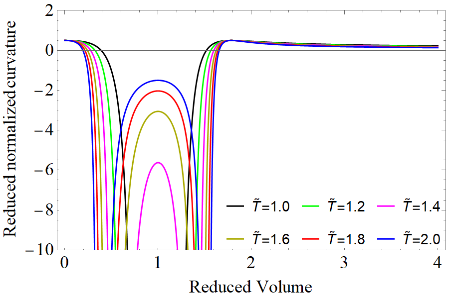
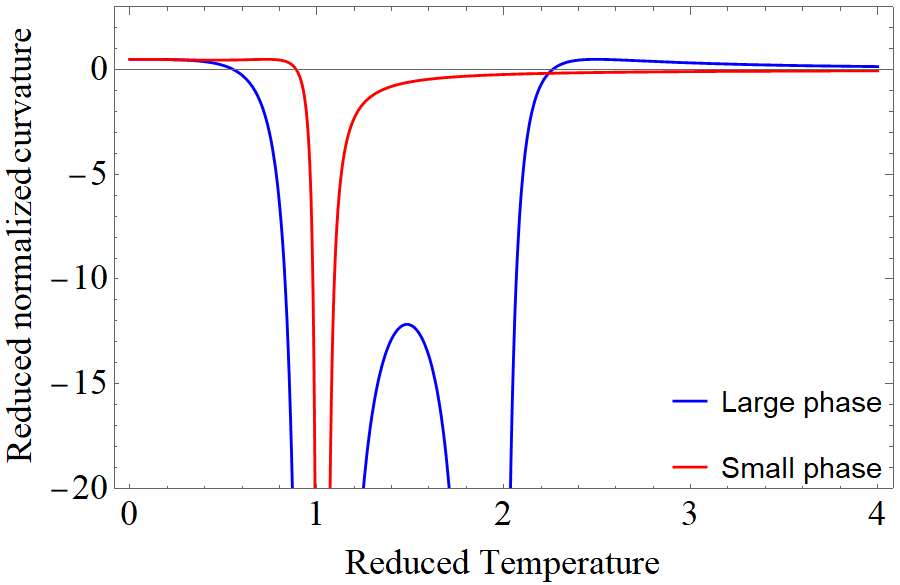
Figure 3: Left panel: The coexistence locus, plotted regarding the reduced volume and temperature. The blue line corresponds to the so-called large phase, while the red one is to the so-called small phase. The black dot is the critical point where these two phases meet. Middle panel: The trend of the reduced normalized curvature versus the reduced volume for different values of $\tilde{T}$ above the critical temperature. As seen (from the right to the left), it is positive, presenting the system as a repulsive interaction. After some point, it becomes negative, meaning the presence of an attractive interaction. Finally, it retakes positive values. This fact accounts for the existence of phase transition. Right panel: Again, the behavior of the reduced normalized curvature, but this time as a function of the reduced temperature at the small and large phases.

where $\{\hat{A}_{i},\hat{B}_{i},\hat{C}_{i}\}$, $i=s,l$, are numerical coefficients. So, from the second relation of Eq. (30) and taking the lower order in $\tau$ of expressions (38), one gets

$$\eta\sim v_{l}-v_{s}\sim(\omega_{l}-\omega_{s})v_{c}\sim|\tau|^{1/2}.$$ (39)

Therefore, the critical exponent $\hat{\beta}$ equals $1/2$. For the critical exponent corresponding to the compressibility $\kappa_{T}$, using (32) up first order,

$$\left(\frac{\partial\tilde{P}}{\partial\tilde{v}}\right)\bigg{|}_{\tau}\simeq\frac{B}{{v}_{c}}\tau,$$ (40)

where $\partial\omega/\partial\tilde{v}=1/v_{c}$ has been used. Then, the third expression in (30) becomes

$$\kappa_{T}\simeq\frac{1}{B\tau}\sim\tau^{-1},$$ (41)

yielding to $\hat{\gamma}=1$. Lastly, by evaluating (32) at the critical temperature, this gives us

$$\tilde{P}-1\sim\omega^{3}\sim\left(\tilde{v}-1\right)^{3},$$ (42)

providing $\hat{\delta}=3$. Collecting all the critical exponent values one has: $\{\hat{\alpha},\hat{\beta},\hat{\gamma},\hat{\delta}\}=\{0,1/2,1,3\}$. These values are the same numerical values predicted for a van der Waals gas. In some sense, this system can be viewed as an inverted van der Waals’s system, that is, the stable branches of a van der Waals’s fluid are permuted by unstable branches for a Kaniadakis’s fluid and vice-versa. Exhibiting both systems is a first-order phase transition with some similarities.

Finally, it is essential to highlight the behavior of the reduced volume against the reduced temperature at the coexistence locus. As can be appreciated in Fig. 3 (left panel), the coexistence curve exhibits the so-called small (red line) and large (blue line) phases, with the black dot as the critical point at which these two phases meet. As the phase transition takes place for those values $\tilde{T}>T_{c}$, the coexistence curves cover this region.

III.3 Ruppeiner’s Geometry

The so-called Ruppeiner’s geometry or geometrothermodynamics Ruppeiner:1981znl ; Ruppeiner:1983zz ; Ruppeiner:1995zz , is a powerful tool to understand the micro-structure of a thermodynamical system better. To do so, it is necessary to compute the scalar curvature (Ricci’s scalar) associated with the following thermodynamics line element

$$\begin{split}dl^{2}=g_{\mu\nu}dx^{\mu}dx^{\nu}\Rightarrow dl^{2}=\frac{1}{T}\bigg{(}-\frac{C_{v}}{T}dT^{2}&\\ +\left(\frac{\partial P}{\partial v}\right)\bigg{|}_{T}dv^{2}\bigg{)}.\end{split}$$ (43)

To obtain the above line element expressed in terms of thermodynamics variables, one needs to endow the geometry with thermodynamical meaning as follows: i) the space-time coordinates $x^{\mu}$ should be functions of the internal energy $U$ and the molar volume $v$, ii) the metric tensor $g_{\mu\nu}$ should be related with the entropy $S$ using $g_{\mu\nu}=-\frac{\partial S^{2}}{\partial x^{\mu}\partial x^{\nu}}$ and iii) express the first thermodynamic law in terms of the entropy $S$ and then use thermodynamics relation among the variables.

Using the reduced pressure (25), the associated reduced Riccis’s scalar $\tilde{\mathcal{R}}$ to the $(\tilde{v},\tilde{T})$-plane described by the line element (43) is given by

$$\tilde{\mathcal{R}}(\tilde{v},\tilde{T})=\frac{\left(\sqrt{3}-\tilde{A}\tilde{v}^{4}\right)\left(\sqrt{3}-\tilde{A}\tilde{v}^{4}-2\sqrt{5}\tilde{v}\tilde{T}+\tilde{B}\tilde{v}^{5}\tilde{T}\right)}{2C_{v}\left(\sqrt{3}-\tilde{A}\tilde{v}^{4}-\sqrt{5}\tilde{v}\tilde{T}+\tilde{B}\tilde{v}^{5}\tilde{T}\right)^{2}},$$ (44)

with $\tilde{A}=5\sqrt{3}-4\sqrt{5}$ and $\tilde{B}=4\sqrt{3}-3\sqrt{5}$.

As in the van der Waals’s gas, here $C_{v}=0$, this makes the line element (43) degenerated, and through $\mathcal{R}$ one can see that this value of the heat capacity at constant volume, constitutes a curvature singularity. A way to solve this issue is to introduce the so-called normalized scalar curvature Wei:2015iwa

$$\tilde{\mathcal{R}}_{N}=C_{v}\tilde{\mathcal{R}}.$$ (45)

In this form (44) becomes

$$\tilde{\mathcal{R}}_{N}(\tilde{v},\tilde{T})=\frac{\left(\sqrt{3}-\tilde{A}\tilde{v}^{4}\right)\left(\sqrt{3}-\tilde{A}\tilde{v}^{4}-2\sqrt{5}\tilde{v}\tilde{T}+\tilde{B}\tilde{v}^{5}\tilde{T}\right)}{2\left(\sqrt{3}-\tilde{A}\tilde{v}^{4}-\sqrt{5}\tilde{v}\tilde{T}+\tilde{B}\tilde{v}^{5}\tilde{T}\right)^{2}},$$ (46)

eliminating the singularity at $C_{v}=0$. However, there is a double point at

$$\tilde{T}_{\text{div}}=\frac{12+3\sqrt{15}+\sqrt{15}\tilde{v}^{4}}{15\tilde{v}+4\sqrt{15}\tilde{v}-3\tilde{v}^{5}}$$ (47)

where $\tilde{\mathcal{R}}_{N}$ diverges. What is more, at the critical point, its behavior is

$$\lim_{(\tilde{v},\tilde{T})\rightarrow(1,1)}\tilde{\mathcal{R}}_{N}(\tilde{v},\tilde{T})\rightarrow-\infty.$$ (48)

In the middle panel of Fig. 3 it is shown the trend of the reduced normalized curvature versus the reduced volume. For $\tilde{T}>1$, this scalar is positive in nature, which means that the system is under a repulsive interaction. Then, as the reduced volume decreases, the reduced normalized curvature becomes negative in nature, implying an attractive interaction. Finally, this scalar again takes positive values for small enough reduced volumes, leading to a repulsive interaction among the particle fluids. Interestingly, there are two divergent points where the scalar curvature goes to negative infinity. With a decrease in temperature, these two divergent points get close, coinciding at $\tilde{T}=1$ (see black line in the middle panel of Fig. 3). This behavior of the reduced normalized curvatures accounts for the thermodynamics phase transition. Besides, as $\tilde{T}$ increases, the magnitude of the reduced normalized curvature $|\tilde{\mathcal{R}}|$ tends to zero.

In terms of the reduced temperature (coexistence locus), the reduced normalized curvature is exhibited in the right panel of Fig. 3. Here, the large phase (blue line) shows (from right to left) regions where the reduced normalized curvatures go from repulsive, attractive, and repulsive zones. On the other hand, the small phase (red line) is negative (attractive interaction). There is a divergent behavior at $\tilde{T}$, and finally, for $\tilde{T}<1$, it becomes positive again (repulsive interaction). So, the attractive behavior and the divergent points are in the coexistence phase. These regions are excluded due to the fact that the equation of state is invalid in the coexistence phase. So, there is only an attractive interaction among the molecules of the fluid.

For values $\tilde{T}\leq 1$, the trend of the reduced normalized curvature is depicted in Fig. 4. In this case, the two divergent points disappear, appearing a negative well-like potential at $\tilde{v}=1$. Moreover, as $\tilde{T}$ decreases in magnitude, this well-like potential is shallower.

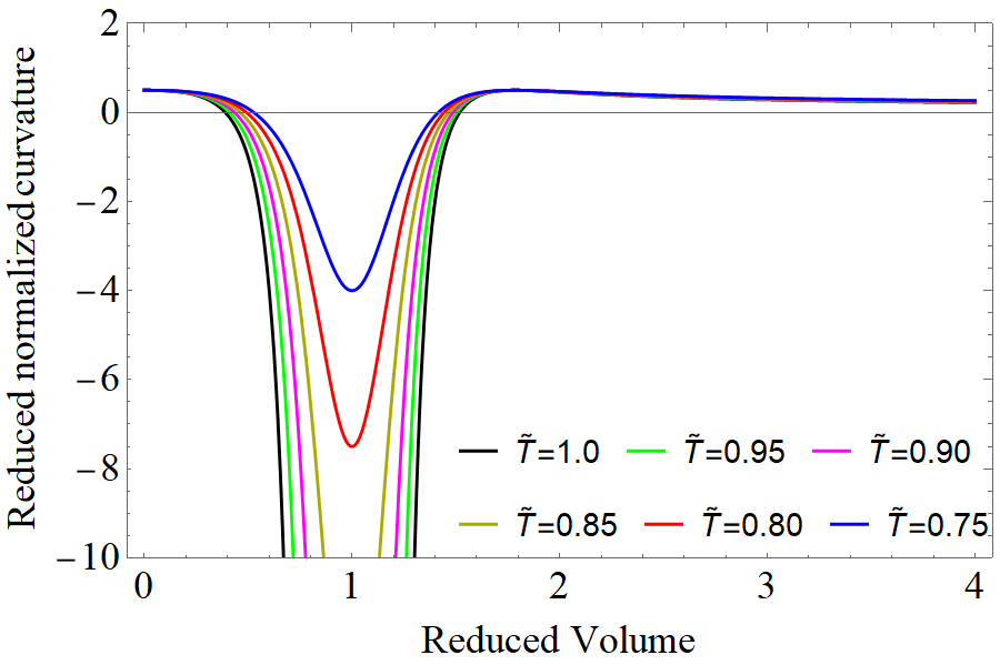
Figure 4: The trend of the reduced normalized scalar curvature $\tilde{\mathcal{R}}_{N}$ versus the reduced volume $\tilde{v}$, for different values of the reduced temperature $\tilde{T}$, starting from the critical one (black line) and values above it. As $\tilde{T}$ decreases in magnitude, the well-like potential formed around the critical point $\{\tilde{v},\tilde{T}\}$ shallower.

Now, it is important to examine the critical exponent of $\tilde{\mathcal{R}}_{N}$ near the critical point along the coexistence curves for small phase (sp) and large phase (lp), which can give us some universal properties of the system. In general, it satisfies

$$\tilde{\mathcal{R}}_{N}\sim-(\tilde{T}-1)^{\hat{\epsilon}}.$$ (49)

Evaluating (46) at (38) and keeping the leading order, one gets

$$\tilde{\mathcal{R}}_{N}(\text{sp})=\tilde{\mathcal{R}}_{N}(\text{lp})=-\frac{1}{8}(\tilde{T}-1)^{-2}+\mathcal{O}(\tilde{T}-1)^{-3/2}.$$ (50)

Therefore, from the above expansion, as $\tilde{T}\rightarrow 1$

$$\tilde{\mathcal{R}}_{N}(\tilde{T}-1)^{2}=-\frac{1}{8}.$$ (51)

This result confirms that near the critical point $\tilde{\mathcal{R}}(\tilde{T}-1)^{2}C_{v}$ has a universal value $-1/8$ and critical exponent $\hat{\epsilon}=2$. Again, these values correspond to those values found for a van der Waals gas Wei:2015iwa . Nevertheless, this system drifts apart from the usual van der Waals gas behavior.

IV Conclusions

This paper studies modified Friedmann equations using Kaniadakis’s entropy, thermodynamics phase transitions, and the microstructure of the FLRW cosmological model.

As a first approach to the problem, we have worked at leading order on the parameter $K$ for the EoS (20). This allows for obtaining analytical solutions for the system. (21). The results show that this model is driven by a stiff matter distribution, subject to a negative absolute temperature (22). These facts reveal that cosmology corresponds to an expanding cosmological era where the AH is an outer-past surface.

The system undergoes a first-order phase transition. This phenomenon takes place for those values greater than the critical temperature $\tilde{T}>T_{c}$. In contrast, for those values below the critical one, the system does not present any drastic change (see left and middle panels in Fig. 1 and Fig. 2 where Gibbs’s free energy displays the swallow tail shape). This behavior is novel, because in comparison with the van der Waals’s fluid, the first order phase transition occurs below the critical point, what is more, here one has a kind of an inverse van der Waals’s system. That is, those regions belonging to the coexistence phase where the van der Waals’s fluid is stable/unstable, in the present case, are unstable/stable. Although these zones are not described by the EoS (25), forbidden regions. On the other hand, for $\tilde{T}<T_{c}$ the system is completely unstable (see right panel in Fig. 1).

The behavior near the critical point shows that the critical exponents obtained the same values for a van der Waals fluid in the mean-field theory. Also, there are small and large phases, as shown in the left panel of Fig 3. From the point of view of Ruppeiner’s geometry, the normalized scalar curvature also has the corresponding van der Waals’s critical exponent. Besides expanding this object around the small and large phases, one obtains the universal constant $-1/8$ at the leading order. At the coexistent phase, the normalized scalar curvature is positive for $\tilde{v}>1$. It becomes negative as $\tilde{v}$ approaches the critical value. Then it is positive again for small $\tilde{v}$. From previous studies, we know that $\tilde{\mathcal{R}}_{N}>0$ means repulsive interaction and $\tilde{\mathcal{R}}_{N}<0$ attractive interaction. Here, the coexistence phase presents both types of interaction among the particles of the system (see middle panel of Fig. 3). However, these states are not valid or covered by the thermodynamics description of the EoS (25). In terms of the reduced temperature at the small and large phases, the trend of $\tilde{\mathcal{R}}_{N}$ is depicted in the right panel of 3. As can be appreciated, there are two divergent points for the large phase, while there is only one divergent point around the critical point for the small one. Furthermore, for the small phase, the normalized scalar curvature changes in sign only once, coming from attractive to repulsive interaction. On the other hand, from Fig. 4, the behavior of $\tilde{\mathcal{R}}_{N}$ versus $\tilde{v}$ for values below the critical point is exhibited. In this case, there is only one divergent point around the critical value $\tilde{v}=v_{c}$. The behavior around the critical point, in this case, resembles a negative well-like potential, where as $\tilde{T}$ decreases in magnitude, this well-like potential is shallower.

To conclude this work, it is worth mentioning that Kaniadakis’s entropy introduces interesting and intriguing modifications to the Friedmann cosmological model from a pure classical thermodynamics description. The results obtained in this research seem to be not very realistic. This is so because the system presents large unstable thermodynamic regions. Perhaps, with additional studies and using the complete entropy instead of expanding it and keeping just the leading order in $K$, one can find a more detailed picture proving more accurate information, requiring this analysis a numerical treatment. On the other hand, from a theoretical point of view in case of the early Universe evolution state were driven by an stiff matter with a negative absolute temperature, the unstable behavior of the system can be matched with the presence of this peculiar matter distribution subject to this unconventional absolute temperature. Therefore, the present thermodynamics description could, in principle, provide an explanation for this strange cosmological evolution era. Nevertheless, further studies are necessary to corroborate it. This issue shall be addressed elsewhere.

References

- (1) G. Kaniadakis, Statistical mechanics in the context of special relativity, Phys. Rev. E 66 (2002) 056125. arXiv:cond-mat/0210467, doi:10.1103/PhysRevE.66.056125.
- (2) G. Kaniadakis, Statistical mechanics in the context of special relativity. II., Phys. Rev. E 72 (2005) 036108. arXiv:cond-mat/0507311, doi:10.1103/PhysRevE.72.036108.
- (3) H. Moradpour, A. H. Ziaie, M. Kord Zangeneh, Generalized entropies and corresponding holographic dark energy models, Eur. Phys. J. C 80 (8) (2020) 732. arXiv:2005.06271, doi:10.1140/epjc/s10052-020-8307-x.
- (4) J. D. Bekenstein, Black holes and entropy, Phys. Rev. D 7 (1973) 2333–2346. doi:10.1103/PhysRevD.7.2333.
- (5) A. Hernández-Almada, G. Leon, J. Magaña, M. A. García-Aspeitia, V. Motta, E. N. Saridakis, K. Yesmakhanova, Kaniadakis-holographic dark energy: observational constraints and global dynamics, Mon. Not. Roy. Astron. Soc. 511 (3) (2022) 4147–4158. arXiv:2111.00558, doi:10.1093/mnras/stac255.
- (6) A. Hernández-Almada, G. Leon, J. Magaña, M. A. García-Aspeitia, V. Motta, E. N. Saridakis, K. Yesmakhanova, A. D. Millano, Observational constraints and dynamical analysis of Kaniadakis horizon-entropy cosmology, Mon. Not. Roy. Astron. Soc. 512 (4) (2022) 5122–5134. arXiv:2112.04615, doi:10.1093/mnras/stac795.
- (7) N. Drepanou, A. Lymperis, E. N. Saridakis, K. Yesmakhanova, Kaniadakis holographic dark energy and cosmology, Eur. Phys. J. C 82 (5) (2022) 449. arXiv:2109.09181, doi:10.1140/epjc/s10052-022-10415-9.
- (8) S. Nojiri, S. D. Odintsov, T. Paul, Early and late universe holographic cosmology from a new generalized entropy, Phys. Lett. B 831 (2022) 137189. arXiv:2205.08876, doi:10.1016/j.physletb.2022.137189.
- (9) S. Nojiri, S. D. Odintsov, V. Faraoni, From nonextensive statistics and black hole entropy to the holographic dark universe, Phys. Rev. D 105 (4) (2022) 044042. arXiv:2201.02424, doi:10.1103/PhysRevD.105.044042.
- (10) S. D. Odintsov, S. D’Onofrio, T. Paul, Holographic realization from inflation to reheating in generalized entropic cosmology (6 2023). arXiv:2306.15225, doi:10.1016/j.dark.2023.101277.
- (11) Sania, N. Azhar, S. Rani, A. Jawad, Cosmic and Thermodynamic Consequences of Kaniadakis Holographic Dark Energy in Brans–Dicke Gravity, Entropy 25 (4) (2023) 576. doi:10.3390/e25040576.
- (12) E. M. C. Abreu, J. A. Neto, Statistical approaches on the apparent horizon entropy and the generalized second law of thermodynamics, Phys. Lett. B 824 (2022) 136803. arXiv:2107.04869, doi:10.1016/j.physletb.2021.136803.
- (13) H. Moradpour, A. H. Ziaie, I. P. Lobo, J. P. Morais Graça, U. K. Sharma, A. S. Jahromi, The third law of thermodynamics, non-extensivity and energy definition in black hole physics, Mod. Phys. Lett. A 37 (12) (2022) 2250076. arXiv:2106.00378, doi:10.1142/S0217732322500766.
- (14) G. Lambiase, G. G. Luciano, A. Sheykhi, Slow-roll inflation and growth of perturbations in Kaniadakis modification of Friedmann cosmology, Eur. Phys. J. C 83 (10) (2023) 936. arXiv:2307.04027, doi:10.1140/epjc/s10052-023-12112-7.
- (15) G. G. Luciano, E. Saridakis, criticalities, phase transitions and geometrothermodynamics of charged AdS black holes from Kaniadakis statistics (8 2023). arXiv:2308.12669.
- (16) S. D. Odintsov, T. Paul, Generalised (non-singular) entropy functions with applications to cosmology and black holes, 2023. arXiv:2301.01013.
- (17) I. Cimidiker, M. P. Dabrowski, H. Gohar, Generalized uncertainty principle impact on nonextensive black hole thermodynamics, Class. Quant. Grav. 40 (14) (2023) 145001. arXiv:2301.00609, doi:10.1088/1361-6382/acdb40.
- (18) A. Lymperis, S. Basilakos, E. N. Saridakis, Modified cosmology through Kaniadakis horizon entropy, Eur. Phys. J. C 81 (11) (2021) 1037. arXiv:2108.12366, doi:10.1140/epjc/s10052-021-09852-9.
- (19) S. Nojiri, S. D. Odintsov, Micro-canonical and canonical description for generalised entropy, Phys. Lett. B 845 (2023) 138130. arXiv:2304.09014, doi:10.1016/j.physletb.2023.138130.
- (20) S. D. Odintsov, T. Paul, A non-singular generalized entropy and its implications on bounce cosmology, Phys. Dark Univ. 39 (2023) 101159. arXiv:2212.05531, doi:10.1016/j.dark.2022.101159.
- (21) S. Nojiri, S. D. Odintsov, T. Paul, Microscopic interpretation of generalized entropy, Phys. Lett. B 847 (2023) 138321. arXiv:2311.03848, doi:10.1016/j.physletb.2023.138321.
- (22) A. Sheykhi, Corrections to Friedmann equations inspired by Kaniadakis entropy (2 2023). arXiv:2302.13012.
- (23) T. Jacobson, Thermodynamics of space-time: The Einstein equation of state, Phys. Rev. Lett. 75 (1995) 1260–1263. arXiv:gr-qc/9504004, doi:10.1103/PhysRevLett.75.1260.
- (24) T. Padmanabhan, Gravity and the thermodynamics of horizons, Phys. Rept. 406 (2005) 49–125. arXiv:gr-qc/0311036, doi:10.1016/j.physrep.2004.10.003.
- (25) T. Padmanabhan, Classical and quantum thermodynamics of horizons in spherically symmetric space-times, Class. Quant. Grav. 19 (2002) 5387–5408. arXiv:gr-qc/0204019, doi:10.1088/0264-9381/19/21/306.
- (26) C. W. Misner, D. H. Sharp, Relativistic equations for adiabatic, spherically symmetric gravitational collapse, Phys. Rev. 136 (1964) B571–B576. doi:10.1103/PhysRev.136.B571.
- (27) L. Smarr, Mass formula for Kerr black holes, Phys. Rev. Lett. 30 (1973) 71–73, [Erratum: Phys.Rev.Lett. 30, 521–521 (1973)]. doi:10.1103/PhysRevLett.30.71.
- (28) J. M. Bardeen, B. Carter, S. W. Hawking, The Four laws of black hole mechanics, Commun. Math. Phys. 31 (1973) 161–170. doi:10.1007/BF01645742.
- (29) S. W. Hawking, Particle Creation by Black Holes, Commun. Math. Phys. 43 (1975) 199–220, [Erratum: Commun.Math.Phys. 46, 206 (1976)]. doi:10.1007/BF02345020.
- (30) G. W. Gibbons, S. W. Hawking, Action Integrals and Partition Functions in Quantum Gravity, Phys. Rev. D 15 (1977) 2752–2756. doi:10.1103/PhysRevD.15.2752.
- (31) S. A. Hayward, General laws of black hole dynamics, Phys. Rev. D 49 (1994) 6467–6474. doi:10.1103/PhysRevD.49.6467.
- (32) S. A. Hayward, Gravitational energy in spherical symmetry, Phys. Rev. D 53 (1996) 1938–1949. arXiv:gr-qc/9408002, doi:10.1103/PhysRevD.53.1938.
- (33) S. A. Hayward, Unified first law of black hole dynamics and relativistic thermodynamics, Class. Quant. Grav. 15 (1998) 3147–3162. arXiv:gr-qc/9710089, doi:10.1088/0264-9381/15/10/017.
- (34) H. Kodama, Conserved Energy Flux for the Spherically Symmetric System and the Back Reaction Problem in the Black Hole Evaporation, Prog. Theor. Phys. 63 (1980) 1217. doi:10.1143/PTP.63.1217.
- (35) V. Faraoni, Cosmological apparent and trapping horizons, Phys. Rev. D 84 (2011) 024003. arXiv:1106.4427, doi:10.1103/PhysRevD.84.024003.
- (36) V. Faraoni, Cosmological and Black Hole Apparent Horizons, Vol. 907, 2015. doi:10.1007/978-3-319-19240-6.
- (37) H. Abdusattar, Insight into the Microstructure of FRW Universe from a P-V Phase Transition, JHEP 09 (2023) 147. arXiv:2304.08348, doi:10.1007/JHEP09(2023)147.
- (38) P. G. S. Fernandes, Gravity with a generalized conformal scalar field: theory and solutions, Phys. Rev. D 103 (10) (2021) 104065. arXiv:2105.04687, doi:10.1103/PhysRevD.103.104065.
- (39) G. Ruppeiner, Application of Riemannian geometry to the thermodynamics of a simple fluctuating magnetic system, Phys. Rev. A 24 (1) (1981) 488. doi:10.1103/PhysRevA.24.488.
- (40) G. Ruppeiner, Thermodynamic Critical Fluctuation Theory?, Phys. Rev. Lett. 50 (1983) 287–290. doi:10.1103/PhysRevLett.50.287.
- (41) G. Ruppeiner, Riemannian geometry in thermodynamic fluctuation theory, Rev. Mod. Phys. 67 (1995) 605–659, [Erratum: Rev.Mod.Phys. 68, 313–313 (1996)]. doi:10.1103/RevModPhys.67.605.
- (42) E. M. C. Abreu, J. Ananias Neto, E. M. Barboza, R. C. Nunes, Jeans instability criterion from the viewpoint of Kaniadakis’ statistics, EPL 114 (5) (2016) 55001. arXiv:1603.00296, doi:10.1209/0295-5075/114/55001.
- (43) E. M. C. Abreu, J. A. Neto, E. M. Barboza, R. C. Nunes, Tsallis and Kaniadakis statistics from the viewpoint of entropic gravity formalism, Int. J. Mod. Phys. A 32 (05) (2017) 1750028. arXiv:1701.06898, doi:10.1142/S0217751X17500282.
- (44) E. M. C. Abreu, J. A. Neto, A. C. R. Mendes, A. Bonilla, Tsallis and Kaniadakis statistics from a point of view of the holographic equipartition law, EPL 121 (4) (2018) 45002. arXiv:1711.06513, doi:10.1209/0295-5075/121/45002.
- (45) E. M. C. Abreu, J. A. Neto, A. C. R. Mendes, R. M. de Paula, Loop Quantum Gravity Immirzi parameter and the Kaniadakis statistics, Chaos, Solitons and Fractals 118 (2019) 307–310. arXiv:1808.01891, doi:10.1016/j.chaos.2018.11.033.
- (46) R.-G. Cai, L.-M. Cao, Unified first law and thermodynamics of apparent horizon in FRW universe, Phys. Rev. D 75 (2007) 064008. arXiv:gr-qc/0611071, doi:10.1103/PhysRevD.75.064008.
- (47) G. Oliveira-Neto, G. A. Monerat, E. V. Correa Silva, C. Neves, L. G. Ferreira Filho, An Early Universe Model with Stiff Matter and a Cosmological Constant, Int. J. Mod. Phys. Conf. Ser. 03 (2011) 254–265. arXiv:1106.3963, doi:10.1142/S2010194511001346.
- (48) T. Banks, Holographic Space-time from the Big Bang to the de Sitter era, J. Phys. A 42 (2009) 304002. arXiv:0809.3951, doi:10.1088/1751-8113/42/30/304002.
- (49) F. T. Falciano, N. Pinto-Neto, E. S. Santini, An Inflationary Non-singular Quantum Cosmological Model, Phys. Rev. D 76 (2007) 083521. arXiv:0707.1088, doi:10.1103/PhysRevD.76.083521.
- (50) J. P. P. Vieira, C. T. Byrnes, A. Lewis, Cosmology with Negative Absolute Temperatures, JCAP 08 (2016) 060. arXiv:1604.05099, doi:10.1088/1475-7516/2016/08/060.
- (51) P. Binétruy, A. Helou, The Apparent Universe, Class. Quant. Grav. 32 (20) (2015) 205006. arXiv:1406.1658, doi:10.1088/0264-9381/32/20/205006.
- (52) A. Helou, Dynamics of the Cosmological Apparent Horizon: Surface Gravity & Temperature (2015). arXiv:1502.04235.
- (53) A. Helou, Dynamics of the four kinds of Trapping Horizons and Existence of Hawking Radiation (2015). arXiv:1505.07371.
- (54) M. Cruz, S. Lepe, Thermodynamics of a transient phantom scenario, Phys. Dark Univ. 42 (2023) 101367. arXiv:2304.02735, doi:10.1016/j.dark.2023.101367.
- (55) N. Goldenfeld, Lectures on phase transitions and the renormalization group, Westview Press, New York, 1992.
- (56) G. Ruppeiner, Thermodynamic curvature and black holes, Springer Proc. Phys. 153 (2014) 179–203. arXiv:1309.0901, doi:10.1007/978-3-319-03774-5_10.
- (57) G. Ruppeiner, Thermodynamic Black Holes, Entropy 20 (6) (2018) 460. arXiv:1803.08990, doi:10.3390/e20060460.
- (58) G. Ruppeiner, A.-M. Sturzu, Black hole microstructures in the extremal limit, Phys. Rev. D 108 (8) (2023) 086004. arXiv:2304.06187, doi:10.1103/PhysRevD.108.086004.
- (59) S.-W. Wei, Y.-X. Liu, Insight into the Microscopic Structure of an AdS Black Hole from a Thermodynamical Phase Transition, Phys. Rev. Lett. 115 (11) (2015) 111302, [Erratum: Phys.Rev.Lett. 116, 169903 (2016)]. arXiv:1502.00386, doi:10.1103/PhysRevLett.115.111302.