On Valid Multivariate Generalizations of the Confluent Hypergeometric Covariance Function

Abstract

Modeling of multivariate random fields through Gaussian processes calls for the construction of valid cross-covariance functions describing the dependence between any two component processes at different spatial locations. The required validity conditions often present challenges that lead to complicated restrictions on the parameter space. The purpose of this paper is to present a simplified techniques for establishing multivariate validity for the recently-introduced Confluent Hypergeometric (CH) class of covariance functions. Specifically, we use multivariate mixtures to present both simplified and comprehensive conditions for validity, based on results on conditionally negative semidefinite matrices and the Schur product theorem. In addition, we establish the spectral density of the CH covariance and use this to construct valid multivariate models as well as propose new cross-covariances. We show that our proposed approach leads to valid multivariate cross-covariance models that inherit the desired marginal properties of the CH model and outperform the multivariate Matérn model in out-of-sample prediction under slowly-decaying correlation of the underlying multivariate random field. We also establish properties of multivariate CH models, including equivalence of Gaussian measures, and demonstrate their use in modeling a multivariate oceanography data set consisting of temperature, salinity and oxygen, as measured by autonomous floats in the Southern Ocean.

Keywords: Argo floats, cross-covariance, multivariate random fields, spectral construction.

1 Introduction

Multivariate random fields are ubiquitous in several different applications, and Gaussian processes remain a popular tool for modeling such data. However, the analysis in multiple dimensions poses some unique challenges: it is not enough to construct a valid univariate covariance function (which must be positive definite), but the entire matrix of marginal and cross-covariances must be valid. Moreover, one ideally should retain flexibility in the marginal covariances and introduce flexibility in the cross-covariances. The second goal often conflicts with the first; to construct a valid joint model, flexibility of the individual covariance functions may be lost. Concerned with this aspect, the traditional thrust in the literature (see, e.g., Gneiting et al.,, 2010; Apanasovich et al.,, 2012) has focused on simple parametric covariance functions, such as Matérn, and considered how to build a valid cross-covariance using this component as the marginal model. The challenge with this approach is that establishing validity for the joint model often leads to complicated and artificial restrictions which must be worked out in a dimension-specific manner. This happens because one considers two processes at a time, and the desired validity conditions are combined post hoc. Thus, the construction of a valid covariance function for two correlated series (e.g., temperature and oxygen over a spatial region) must be re-done when one adds a third (e.g., temperature, oxygen, and salinity over the same region).

In this paper, we establish validity conditions primarily using the approach of multivariate mixtures. Although the mixture approach has attracted some recent attention (Emery et al.,, 2022; Emery and Porcu,, 2023, and others), it remains relatively obscure compared to the two-at-a-time approaches mentioned above. However, the chief benefit here is that (a) conditions of validity can be established in an identical manner regardless of the dimension one is dealing with and (b) it is still possible to allow considerable flexibility in the marginal and cross-covariance terms.

The chief focus of the current paper is the recently proposed Confluent Hypergeometric (CH) family of covariance functions (Ma and Bhadra,, 2022), that rectifies one significant limitation of the Matérn class. The main reason for the popularity of Matérn over other covariances is the precise control over the degree of mean square differentiability of the associated random process (see, e.g., Chapter 2 of Stein,, 1999). However, the Matérn class possesses exponentially decaying tails, which could be too fast a rate of decay for some applications. Other covariances such as the generalized Cauchy class admit polynomial tails, at the expense of allowing no control over the degree of mean square differentiability. The CH class allows the best of both worlds: it contains two parameters that control the degree of mean squared differentiability and the polynomial tail decay rate, respectively, that are independent of each other. The CH class has demonstrated considerable success in one dimension over the Matérn class in simulations and in the analysis of atmospheric CO₂ data (Ma and Bhadra,, 2022). A valid multivariate generalization, however, has so far remained elusive. This is the gap that the current article closes.

Since the CH covariance is a continuous mixture of the Matérn covariance (Ma and Bhadra,, 2022), demonstrating validity of the multivariate model through a continuous mixture of a multivariate Matérn model is a natural approach. Using this, we introduce a valid model that provides full flexibility in the origin behavior, tail behavior, and scale of each of the marginal covariances, as well as flexibility in the origin behavior and scale of the cross-covariances. In addition, we establish the spectral density of the CH covariance at all frequencies, whereas Ma and Bhadra, (2022) only provided results on the tail behavior of the spectral density. This gives us additional tools to ensure validity of the multivariate covariance and construct new cross-covariance models. Recently, Yarger et al., (2023) proposed using the spectral density to construct asymmetric multivariate Matérn models. Inspired by this approach, we provide constructive techniques for flexible asymmetric CH cross-covariances in the current paper.

We compare multivariate CH and Matérn models in simulation studies and an analysis of an oceanography data set. Similar to results in Ma and Bhadra, (2022), the multivariate CH covariance provides advantages when there are larger gaps between the spatial locations of observations. In our data analysis, we focus on oceanographic temperature, salinity, and oxygen data collected by devices called floats. We plot the oxygen data used in Figure 1, which comes from the Southern Ocean Carbon and Climate Observations and Modeling (SOCCOM) project (Johnson et al.,, 2020). The SOCCOM project is part of the larger Argo project dedicated to float-based monitoring of the oceans (Wong et al.,, 2020; Argo,, 2023). We include data from the months of February, March, and April over the years 2017-2023, resulting in 436 total locations. Since there are a limited number of such floats, gaps between observations are very often hundreds of kilometers apart. However, leveraging available temperature and salinity data (which are more abundant) should be expected to improve predictions of oxygen, suggesting that a multivariate data analysis is useful. Through the models we established, the multivariate relationship between these variables can be flexibly estimated, including varying polynomial tail decay behavior of the marginal covariances.

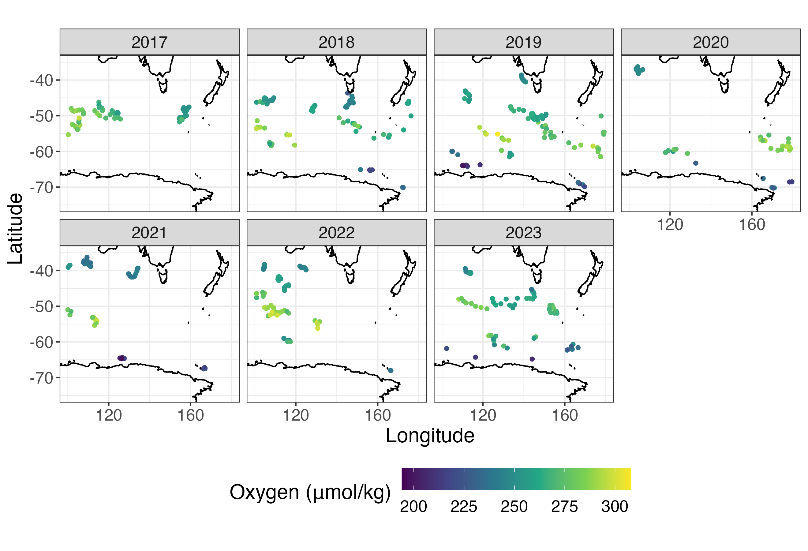
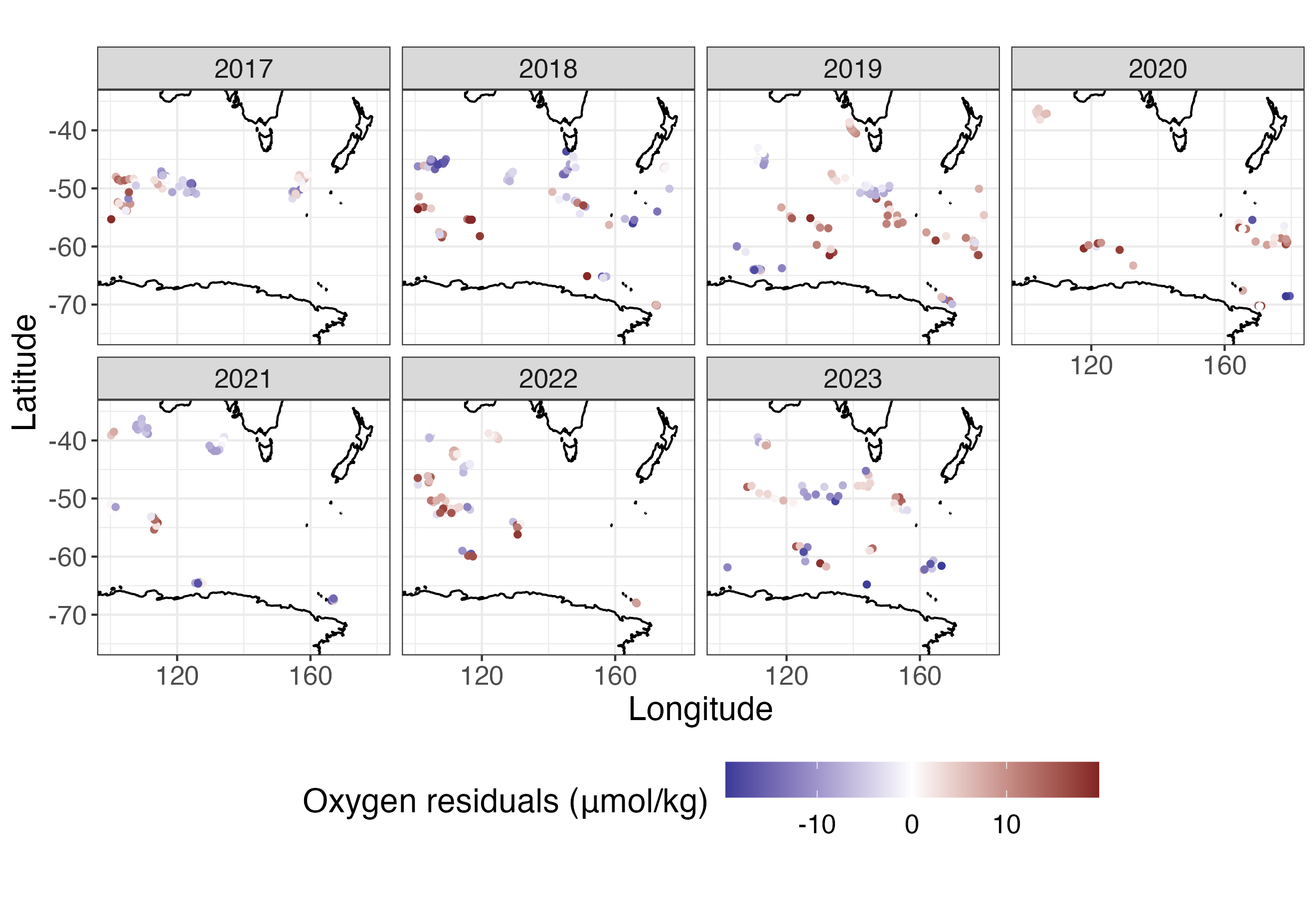
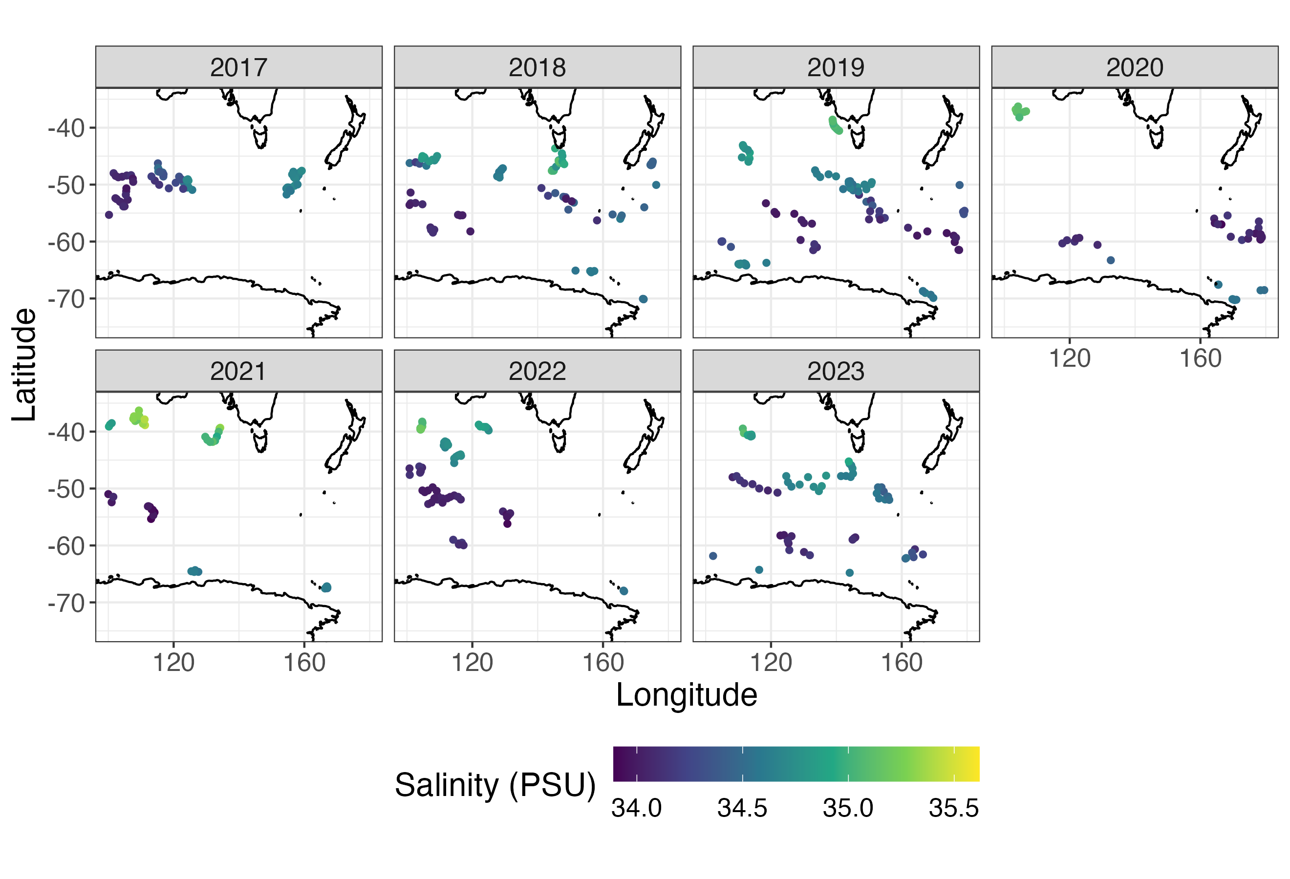
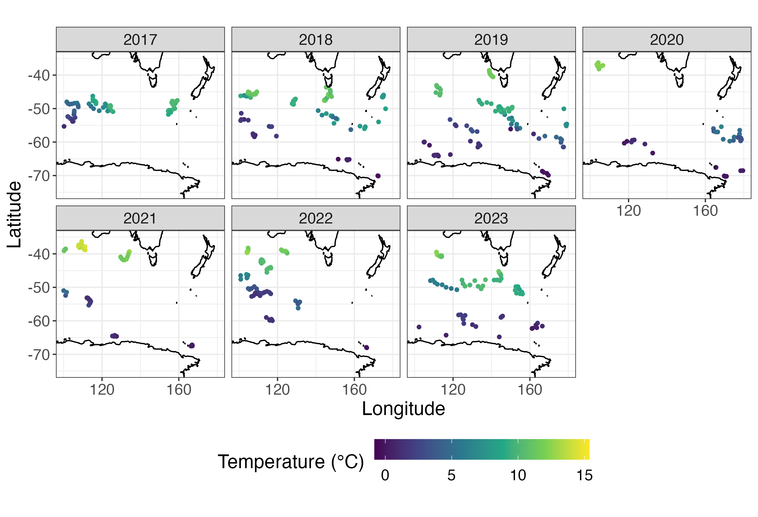
Figure 1: Oxygen (Top), salinity (Middle), and temperature (Bottom) measurements taken at 150 meters deep in the ocean during the months of February, March, and April, which were used in the data application. (Left) Original data and (Right) residuals computed after estimating a spatially-varying mean.

The rest of the paper is organized as follows. In Section 2, we review some background material on the univariate CH and Matérn classes for Gaussian random fields. We also provide the new result on the spectral density of the CH class in Section 2.1. The main topic of this paper: valid multivariate generalizations of the CH class is discussed in Section 3. Extensive simulations supporting the theory are discussed in Section 4, followed by the analysis of multivariate oceanography data in the Southern Ocean in Section 5. We conclude with some future directions in Section 6.

1.1 Notations and preliminaries

We use $\odot$ to denote the Hadamard, or entry-wise product of two matrices of the same dimension. In some sections (as specified later), we omit this notation and take all matrix operations entry-wise. We denote $f(z)\overset{z\to\infty}{\asymp}g(z)$ to mean $\lim_{z\to\infty}{f(z)}/{g(z)}=c$ for some $c\in(0,\infty)$, while the notation $f(z)\overset{z\to\infty}{\sim}g(z)$ is reserved for the case $c=1$. Let $\lVert x\rVert=\sqrt{\sum_{i=1}^{d}x_{i}}$ be the Euclidean norm in $d$ dimensions. For a scalar $z$, let $\lfloor z\rfloor$ denote the floor function, the largest integer less than or equal to $z$. Let $\Gamma(z)$ denote the Gamma function and $B(a,b)=\Gamma(a)\Gamma(b)/\Gamma(a+b)$ denote the Beta function.

2 Review of Univariate CH and Matérn Classes and New Results on CH Spectral Density

We begin with a discussion of the Matérn covariance model, a celebrated and commonly-used class of covariance functions in spatial statistics; a comprehensive overview of this model and its extensions is given in Porcu et al., (2023). In general, a covariance function models the covariance between a process at different locations. For a process $Y(s)$ for $s\in\mathbb{R}^{d}$, a commonly-used assumption in spatial statistics is that $\mathbb{E}(Y(s))=0$ and $\mathbb{E}[Y(s)Y(t)]=C(t-s;\theta)$ for all $s,t\in\mathbb{R}^{d}$ and $C(\cdot;\theta)$ is a covariance function. This is often referred to as “second-order” stationarity. For a vector $h\in\mathbb{R}^{d}$ and parameters $\nu>0$, $\phi>0$, and $\sigma^{2}>0$, the Matérn model may be defined as:

$$C(h;\theta)=\mathcal{M}(h;\nu,\phi,\sigma^{2}) =\sigma^{2}\frac{2^{1-\nu}}{\Gamma(\nu)}\left(\frac{\lVert h\rVert}{\phi}\right)^{\nu}\mathcal{K}_{\nu}\left(\frac{\lVert h\rVert}{\phi}\right),$$

where $\mathcal{K}_{\nu}(\cdot)$ is the modified Bessel function of the second kind (see, e.g., Stein,, 1999). We use a slightly different parameterization of the Matérn model compared to Ma and Bhadra, (2022). Therefore, later results and construction for the Confluent Hypergeometric covariance is slightly different than in Ma and Bhadra, (2022). The spectral density of the Matérn model is

$$f_{\mathcal{M}}(x;\nu,\phi,\sigma^{2}) =\sigma^{2}\frac{\Gamma(\nu+\frac{d}{2})}{\pi^{\frac{d}{2}}\Gamma(\nu)\phi^{2\nu}}\left(\phi^{-2}+\lVert x\rVert^{2}\right)^{-\nu-\frac{d}{2}},$$ (1)

so that $\mathcal{M}(h;\nu,\phi,\sigma^{2})=\int_{\mathbb{R}^{d}}e^{\mathbbm{i}h^{\top}x}f_{\mathcal{M}}(x;\nu,\phi,\sigma^{2})dx$. In the Matérn model, the parameter $\sigma^{2}$ controls the marginal variance of the resulting process: $\mathcal{M}(0;\nu,\phi,\sigma^{2})=\sigma^{2}$. The parameter $\nu$ is called the smoothness parameter due to the property that $Y(s)$ is $\lfloor\nu\rfloor$-times mean-square differentiable. Finally, the parameter $\phi$ is a range parameter controlling how fast the covariance decays. In particular, since $\mathcal{K}_{\nu}(z)\overset{|z|\to\infty}{\sim}\sqrt{\pi/(2|z|)}\textrm{exp}(-|z|)$ (DLMF,, 2021), we have:

$$\mathcal{M}(h;\nu,\phi,\sigma^{2})\overset{\lVert h\rVert\to\infty}{\sim}\sigma^{2}2^{\frac{1}{2}-\nu}\sqrt{\pi}\left(\frac{\lVert h\rVert}{\phi}\right)^{\nu-\frac{1}{2}}\textrm{exp}\left(-\frac{\lVert h\rVert}{\phi}\right).$$

For large $\lVert h\rVert$, the covariance then primarily decays exponentially.

However, in many settings, covariances with slower decay may be desired. With this in mind, Ma and Bhadra, (2022) introduced a “Confluent Hypergeometric” covariance class, defined as

$$\mathcal{CH}(h;\nu,\alpha,\beta,\sigma^{2}) =\frac{\beta^{2\alpha}}{2^{\alpha}\Gamma(\alpha)}\int_{0}^{\infty}\mathcal{M}(h;\nu,\phi,\sigma^{2})\phi^{-2\alpha-2}\textrm{exp}\left(-\frac{\beta^{2}}{2\phi^{2}}\right)d\phi^{2}$$

$$=\sigma^{2}\frac{\Gamma(\nu+\alpha)}{\Gamma(\nu)}\mathcal{U}\left(\alpha,1-\nu,\frac{\lVert h\rVert^{2}}{2\beta^{2}}\right),$$

where $\mathcal{U}(a,b,z)$ represents a confluent hypergeometric function of the second kind (see, e.g., Chapter 13 of DLMF,, 2021). We refer to $\mathcal{CH}(h;\nu,\alpha,\beta,\sigma^{2})$ as a CH covariance. The CH covariance is obtained as a mixture of the Matérn covariance over the parameter $\phi^{2}$ with respect to an inverse gamma distribution with parameters $\alpha$ and $\beta^{2}/2$. When the marginal covariance of $Y(s)$ is CH, $\nu$ continues to control the smoothness of the process, while the parameter $\alpha$ controls the tail decay of the covariance or the long range dependence of the covariance. In particular,

$$\mathcal{CH}(h;\nu,\alpha,\beta,\sigma^{2})\overset{\lVert h\rVert\to\infty}{\sim}\sigma^{2}\frac{\Gamma(\nu+\alpha)2^{\alpha}}{\Gamma(\nu)}\left(\frac{\lVert h\rVert}{\beta}\right)^{-2\alpha},$$

using 13.2.6 of DLMF, (2021), which establishes that $\mathcal{U}(a,b,z)\overset{z\to\infty}{\sim}z^{-a}$ for $z\in\mathbb{R}$. The parameter $\beta$ in the CH covariance plays a similar role to $\phi$ in the Matérn covariance, so we refer to it as a range parameter.

2.1 Spectral density of the univariate isotropic CH class

While the tail decay of the spectral density of the CH covariance was presented in Ma and Bhadra, (2022), we now present in full generality the spectral density of the CH covariance when $\alpha>d/2$ (as noted in Ma and Bhadra,, 2022, the spectral density is infinite when $0<\alpha\leq d/2$).

Proposition 2.1 (Spectral density of CH covariance).

Suppose that $\alpha>\frac{d}{2}$. Then the spectral density of the univariate CH covariance is

$$f_{\mathcal{CH}}(x;\nu,\alpha,\beta,\sigma^{2}) =\sigma^{2}\frac{\Gamma(\nu+\frac{d}{2})\beta^{d}}{(2\pi)^{d/2}B(\alpha,\nu)}\mathcal{U}\left(\nu+\frac{d}{2},1-\alpha+\frac{d}{2},\frac{\beta^{2}\lVert x\rVert^{2}}{2}\right).$$

We present a concise proof in Section S.1.2. We offer a few comments on this result here. Due to the asymptotic expansion of $\mathcal{U}(a,c,z)\overset{z\to\infty}{\sim}z^{-a}$ (13.2.6, DLMF,, 2021), our expression matches the tail of the spectral density found in Ma and Bhadra, (2022). Notice that the form of the CH covariance and its spectral density have opposite forms in the arguments of $\mathcal{U}$. While $\nu$ controls the origin behavior of the covariance and the tail behavior of the spectral density, $\alpha$ controls the tail behavior of the covariance and the origin behavior of the spectral density. The exact form of the spectral density gives us additional tools to construct and simulate valid multivariate CH processes, which is the primary focus on this work.

3 Construction of Valid Multivariate CH Cross-Covariance Models and Their Properties

To begin, we first discuss a few approaches for constructing valid multivariate Matérn models. Unsurprisingly, we use them later to develop multivariate CH models. In the multivariate case, we have that $Y(s)$ is vector-valued: $\boldsymbol{Y}(s)=[Y_{1}(s),Y_{2}(s),\dots,Y_{p}(s)]^{\top}$. Similarly, instead of a scalar-valued covariance function $C(h;\theta)$, we now deal with a matrix-valued covariance function $\mathbb{E}[\boldsymbol{Y}(s+h)\boldsymbol{Y}(s)^{\top}]=\boldsymbol{C}(h;\boldsymbol{\theta})=[C_{jk}(h;\boldsymbol{\theta})]_{j,k=1}^{p}$, where $C_{jj}(h;\boldsymbol{\theta})$ are referred to as the marginal covariance functions, and $C_{jk}(h;\boldsymbol{\theta})$ for $j\neq k$ are the cross-covariance functions that describe the covariance between $Y_{j}(s+h)$ and $Y_{k}(s)$.

A primary concern in the construction of multivariate Matérn models has been ensuring the validity of the model. In particular, for any $n\in\mathbb{N}$ and any unique set of points $\{s_{1},s_{2},\dots,s_{n}\}$ with $s_{i}\in\mathbb{R}^{d}$, one must ensure that $\sum_{i_{1}=1}^{n}\sum_{i_{2}=1}^{n}y_{i_{1}}y_{i_{2}}\boldsymbol{C}(s_{i_{1}}-s_{i_{2}};\boldsymbol{\theta})$ is symmetric and positive semidefinite for any vector $y=(y_{1},y_{2},\dots,y_{n})\in\mathbb{C}^{n}$; see Section 2 of Yarger et al., (2023). A multivariate version of Bochner’s theorem establishes that one can use the spectral representation to determine if a model is valid (cf. Theorem 2.2 of Yarger et al.,, 2023). If the spectral densities for each component are available, that is,

$$\boldsymbol{C}(h;\boldsymbol{\theta}) =\int_{\mathbb{R}^{d}}e^{\mathbbm{i}h^{\top}x}\boldsymbol{f}(x;\boldsymbol{\theta})dx,$$

where $\boldsymbol{f}(x;\boldsymbol{\theta})=[f_{jk}(x;\boldsymbol{\theta})]_{j,k=1}^{p}$, $\boldsymbol{C}(h;\boldsymbol{\theta})$ may be shown to be valid if $\boldsymbol{f}(x;\boldsymbol{\theta})$ is Hermitian and positive semidefinite for all $x\in\mathbb{R}^{d}$. We refer to $\boldsymbol{f}(x;\boldsymbol{\theta})$ as a matrix-valued spectral density and $f_{jk}(x;\boldsymbol{\theta})$ as the spectral density for the $j,k$ component.

Initially, Gneiting et al., (2010) proposed multivariate Matérn models with Matérn-like cross-covariances and used the spectral density of the Matérn class to establish a valid model, which was generalized in Bevilacqua et al., (2015). For the Matérn model, we take:

$$\boldsymbol{C}(h;\boldsymbol{\theta}) =[\mathcal{M}(h;\nu_{jk},\phi_{jk},\sigma_{jk})]_{j,k=1}^{p};$$ (2)

for parameters $\{\sigma_{jk},\nu_{jk},\phi_{jk}\}_{j,k=1}^{p}$ and $\sigma_{jk}=\sigma_{kj}$, $\nu_{jk}=\nu_{kj}$, and $\phi_{jk}=\phi_{kj}$ for all $j$ and $k$. Here, the diagonal entries $\sigma_{jj}$ now represent the marginal variances of each of the processes, and $\sigma_{jk}$ for $j\neq k$ represent the marginal cross-covariances. Gneiting et al., (2010) and Apanasovich et al., (2012) established conditions for the validity of this model by using the spectral densities $\boldsymbol{f}(x;\boldsymbol{\theta})=[f_{\mathcal{M}}(x;\nu_{jk},\phi_{jk},\sigma_{jk})]_{j,k=1}^{p}$. At times, however, these conditions are quite technical.

Recently, Yarger et al., (2023) proposed to instead construct multivariate Matérn models beginning with the spectral density. In particular, they proposed taking $f_{jk}(x;\boldsymbol{\theta})=\sigma_{jk}f_{\mathcal{M}}(x;\nu_{j},\phi_{j},1)^{\frac{1}{2}}f_{\mathcal{M}}(x;\nu_{k},\phi_{k},1)^{\frac{1}{2}}$. Validity of the model is immediate as long as the matrix $\boldsymbol{\sigma}=[\sigma_{jk}]_{j,k=1}^{p}$ is positive semidefinite. Furthermore, there is flexibility in choosing which square root of the Matérn spectral density to use. Yarger et al., (2023) also introduced cross-covariance functions that have more flexible variance parameterization, resulting in asymmetric forms of the cross-covariance. In only certain cases will the resulting covariance be proportional to a Matérn class. We refer to this approach of constructing valid cross-covariance functions as “spectrally-generated.” Construction in the spectral domain makes validity conditions of the model simple; however, closed-form expressions of the covariance may not always be attainable and may need to be computed through fast Fourier transforms. The approaches of Gneiting et al., (2010) and Yarger et al., (2023) both rely on the spectral density to ensure validity.

In addition to using the spectral density, validity for multivariate Matérn models with form (2) has been shown using a mixture representation of the Matérn covariance, most notably in Emery et al., (2022). In particular, we define a model

$$\boldsymbol{C}(h;\boldsymbol{\theta}) =\int_{0}^{\infty}\boldsymbol{C}_{*}(h;\boldsymbol{\theta},u)\odot\boldsymbol{p}(u|\boldsymbol{\theta})du,$$

where $\boldsymbol{C}_{*}(h;\boldsymbol{\theta},u)$ is a multivariate covariance function that has parameter $u$, and $\boldsymbol{p}(u|\boldsymbol{\theta})$ is a matrix of probability density functions. Then, if $\boldsymbol{C}_{*}(h;\boldsymbol{\theta},u)$ is a valid multivariate covariance for all $u\in(0,\infty)$, and the matrix of $\boldsymbol{p}(u|\boldsymbol{\theta})$ is positive semidefinite for all $u\in(0,\infty)$, the resulting covariance $\boldsymbol{C}(h;\boldsymbol{\theta})$ is also valid (Emery et al.,, 2022). Since the CH covariance is a mixture of the Matérn covariance, one can construct a valid multivariate CH covariance with a mixture of a valid multivariate Matérn model.

We begin by proposing a class of models constructed in the same way as (2) by using cross-covariances that are proportional to CH covariance functions.

3.1 A valid multivariate CH model

Consider a multivariate covariance model with entries $\mathcal{CH}(h;\nu_{jk},\alpha_{jk},\beta_{jk},\sigma_{jk})$. Throughout, assume $\alpha_{jk}>0$, $\beta_{jk}>0$, $\nu_{jk}>0$, and $\sigma_{jj}>0$ for each $j$ and $k$. Let $\boldsymbol{\sigma}=[\sigma_{jk}]$, $\boldsymbol{\nu}=[\nu_{jk}]$, $\boldsymbol{\alpha}=[\alpha_{jk}]$, and $\boldsymbol{\beta}=[\beta_{jk}]$ be $p\times p$ matrices represented by the parameters. In this Subsection, as well as Subsections 3.2 and 3.3, take all matrix operations elementwise. For example, $\Gamma(\boldsymbol{\nu})=[\Gamma(\nu_{jk})]$ and $\mathcal{CH}(h;\boldsymbol{\nu},\boldsymbol{\alpha},\boldsymbol{\beta},\boldsymbol{\sigma})=\left[\mathcal{CH}(h;\nu_{jk},\alpha_{jk},\beta_{jk},\sigma_{jk})\right]_{j,k=1}^{p}$. Before discussing validity conditions, we list a few properties of the multivariate covariance:

• Tail decay: The tail decay of multivariate covariance is,

  $$\mathcal{CH}(h;\boldsymbol{\nu},\boldsymbol{\alpha},\boldsymbol{\beta},\boldsymbol{\sigma})\overset{\lVert h\rVert\to\infty}{\sim}\boldsymbol{\sigma}\frac{2^{\boldsymbol{\alpha}}\Gamma(\boldsymbol{\nu}+\boldsymbol{\alpha})}{\Gamma(\boldsymbol{\nu})}\left(\frac{\lVert h\rVert}{\boldsymbol{\beta}}\right)^{-2\boldsymbol{\alpha}}.$$

  This follows from the asymptotic expansion of $\mathcal{U}(a,b,z)$ discussed above and matches the results in Ma and Bhadra, (2022).

• Smoothness: The $j$-th process is $\lfloor\nu_{jj}\rfloor$ times continuously differentiable. This follows from Ma and Bhadra, (2022).

• Spectral density: The multivariate spectral density of the model is,

  $$\boldsymbol{\sigma}\frac{\Gamma(\boldsymbol{\nu}+\frac{d}{2})\boldsymbol{\beta}^{d}}{(2\pi)^{d/2}B(\boldsymbol{\alpha},\boldsymbol{\nu})}\mathcal{U}\left(\boldsymbol{\nu}+\frac{d}{2},1-\boldsymbol{\alpha}+\frac{d}{2},\boldsymbol{\beta}^{2}\frac{\lVert x\rVert^{2}}{2}\right),$$

  which follows directly from Proposition 2.1.

• Tail behavior of spectral density: As $\lVert x\rVert\to\infty$, the spectral density decays like:

  $$\boldsymbol{\sigma}\frac{\Gamma(\boldsymbol{\nu}+\frac{d}{2})2^{\boldsymbol{\nu}}}{\boldsymbol{\beta}^{2\boldsymbol{\nu}}B(\boldsymbol{\alpha},\boldsymbol{\nu})\pi^{d/2}}\lVert x\rVert^{-2\boldsymbol{\nu}-d}.$$ (3)

  This follows from 13.2.6 of DLMF, (2021).

Such properties may only be useful if we have a valid model. We now give one class of valid models of this form. For easier notation, set $\nu_{j}=\nu_{jj}$, $\alpha_{j}=\alpha_{jj}$, and $\beta_{j}=\beta_{jj}$.

Theorem 3.1.

Suppose that $\nu_{jk}=(\nu_{j}+\nu_{k})/2$, $\alpha_{jk}=(\alpha_{j}+\alpha_{k})/2$, and $\beta_{jk}^{2}=(\beta_{j}^{2}+\beta_{k}^{2})/2$ for all $j\neq k$. Then the multivariate model defined by $\mathcal{CH}(h;\nu_{jk},\alpha_{jk},\beta_{jk},\sigma_{jk})$ is valid if

$$\boldsymbol{\sigma}\boldsymbol{\beta}^{2\boldsymbol{\alpha}}\frac{\Gamma(\boldsymbol{\nu}+\frac{d}{2})}{\Gamma(\boldsymbol{\nu})\Gamma(\boldsymbol{\alpha})}=\left[\sigma_{jk}\left(\frac{\beta_{j}^{2}+\beta_{k}^{2}}{2}\right)^{\frac{\alpha_{j}+\alpha_{k}}{2}}\frac{\Gamma(\frac{\nu_{j}+\nu_{k}}{2}+\frac{d}{2})}{\Gamma(\frac{\nu_{j}+\nu_{k}}{2})\Gamma(\frac{\alpha_{j}+\alpha_{k}}{2})}\right]_{j,k=1}^{p};$$ (4)

is positive semidefinite.

Proof.

In this case, we begin with the valid parsimonious multivariate Matérn, where $\nu_{jk}=(\nu_{j}+\nu_{k})/2$ and $\phi_{jk}=\phi$ for all $j$ and $k$:

$$\boldsymbol{\sigma}\frac{2^{1-\boldsymbol{\nu}}}{\Gamma(\boldsymbol{\nu})}\left(\frac{h}{\phi}\right)^{\boldsymbol{\nu}}\mathcal{K}_{\boldsymbol{\nu}}\left(\frac{h}{\phi}\right),$$

which is known to be valid if the matrix $\boldsymbol{\sigma}\frac{\Gamma(\boldsymbol{\nu}+\frac{d}{2})}{\Gamma(\boldsymbol{\nu})}$ is positive semidefinite (Gneiting et al.,, 2010). We then consider the multivariate covariance of:

$$\int_{0}^{\infty}\boldsymbol{\sigma}\frac{2^{1-\boldsymbol{\nu}}}{\Gamma(\boldsymbol{\nu})}\left(\frac{h}{\phi}\right)^{\boldsymbol{\nu}}\mathcal{K}_{\boldsymbol{\nu}}\left(\frac{h}{\phi}\right)\frac{\boldsymbol{\beta}^{2\boldsymbol{\alpha}}}{2^{\boldsymbol{\alpha}}\Gamma(\boldsymbol{\alpha})}\phi^{-2\boldsymbol{\alpha}-2}\textrm{exp}\left(-\boldsymbol{\beta}^{2}/(2\phi^{2})\right)d\phi^{2}.$$

This is a scale-mixture of the parsimonious multivariate Matérn model, and it is valid if:

$$\boldsymbol{\sigma}\frac{\Gamma(\boldsymbol{\nu}+\frac{d}{2})}{\Gamma(\boldsymbol{\nu})}\frac{\boldsymbol{\beta}^{2\boldsymbol{\alpha}}}{\Gamma(\boldsymbol{\alpha})}\times\left(\sqrt{2}\phi\right)^{-2\boldsymbol{\alpha}}\phi^{-2}\textrm{exp}\left(-\boldsymbol{\beta}^{2}/(2\phi^{2})\right),$$ (5)

is positive semidefinite for all $\phi^{2}>0$, combining the validity conditions of the parsimonious multivariate Matérn and rearranging the term $\phi^{-2\boldsymbol{\alpha}-2}/2^{\boldsymbol{\alpha}}$. See Emery et al., (2022) and Alegría et al., (2019) for examples of constructing valid multivariate models for scale-mixtures of valid covariances. Consider left and right multiplication of (5) by the matrix

$$\textrm{diag}\left(\left[\sqrt{2}\phi\right]^{\alpha_{j}}\times\phi\times\textrm{exp}\left(\frac{\beta_{j}^{2}}{4\phi^{2}}\right),j=1,\dots,p\right),$$

and instead of checking the positive semidefiniteness of (5), we may check the positive semidefiniteness of the resulting matrix, which has $j$, $k$ entry:

$$\sigma_{jk}\frac{\Gamma(\nu_{jk}+\frac{d}{2})}{\Gamma(\nu_{jk})}\frac{\beta_{jk}^{2\alpha_{jk}}}{\Gamma(\alpha_{jk})}\times\left(\sqrt{2}\phi\right)^{-2\alpha_{jk}+\alpha_{j}+\alpha_{k}}\textrm{exp}\left(-\frac{1}{2\phi^{2}}\left[\beta_{jk}^{2}-\frac{(\beta_{j}^{2}+\beta_{k}^{2})}{2}\right]\right).$$

Then, the choice of $\alpha_{jk}=(\alpha_{j}+\alpha_{k})/2$ and $\beta_{jk}^{2}=(\beta_{j}^{2}+\beta_{k}^{2})/2$ leads to the terms to the right of $\times$ dropping out, resulting in a matrix with $j$, $k$ entry:

$$\sigma_{jk}\frac{\Gamma(\nu_{jk}+\frac{d}{2})}{\Gamma(\nu_{jk})}\frac{\beta_{jk}^{2\alpha_{jk}}}{\Gamma(\alpha_{jk})},$$

giving us the condition in (4). ∎

This choice gives simple validity conditions and eliminates the need to estimate additional parameters $\nu_{jk}$, $\alpha_{jk}$, and $\beta_{jk}$ for $j\neq k$, while allowing the different covariances to have different $\nu_{j}$, $\alpha_{j}$, and $\beta_{jj}$ values. In some ways, it is similar to the parsimonious multivariate Matérn model of Gneiting et al., (2010), but this model also allows the tail behavior and the scale parameter to vary for each process. Through the mixing approach, we do not rely on the assumption that $\alpha_{j}>d/2$ for each $j$ (in contrast to Proposition 2.1). Also, we may relax the requirement on $\beta_{jk}$ straightforwardly. Based on the definition and properties of a conditionally negative semidefinite matrix (reviewed in Section S.1 and Emery et al.,, 2022), we may take $\boldsymbol{\beta}^{2}$ to be any conditionally negative semidefinite matrix. This allows $\beta_{jk}^{2}\geq(\beta_{j}^{2}+\beta_{k}^{2})/2$, for example.

Notice that the conditions for validity are similar to previous work on the multivariate Matérn in Gneiting et al., (2010), Apanasovich et al., (2012), and Emery et al., (2022). The term $\boldsymbol{\beta}^{2\boldsymbol{\alpha}}$ involves the scale parameters raised to a power; however, instead of raised to the power $2\boldsymbol{\nu}$ (as in, e.g., Example 3 of Emery et al.,, 2022), $\boldsymbol{\beta}$ is raised to the power $2\boldsymbol{\alpha}$. The term $\Gamma(\boldsymbol{\nu}+d/2)/\Gamma(\boldsymbol{\nu})$ results immediately from mixing the valid parsimonious multivariate Matérn model. We additionally have $1/\Gamma(\boldsymbol{\alpha})$, a remnant from the inverse gamma mixing distribution. These conditions suggest that processes with different smoothnesses, tail decay, or scale parameters cannot be perfectly correlated.

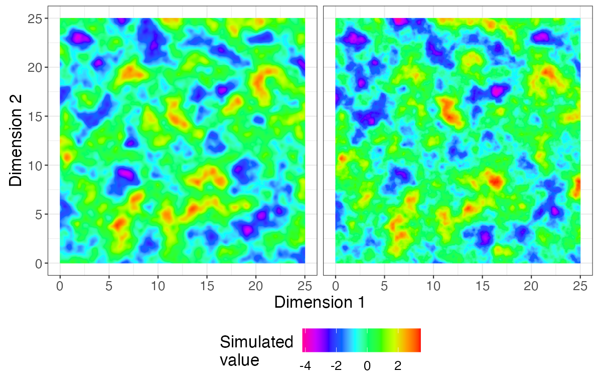
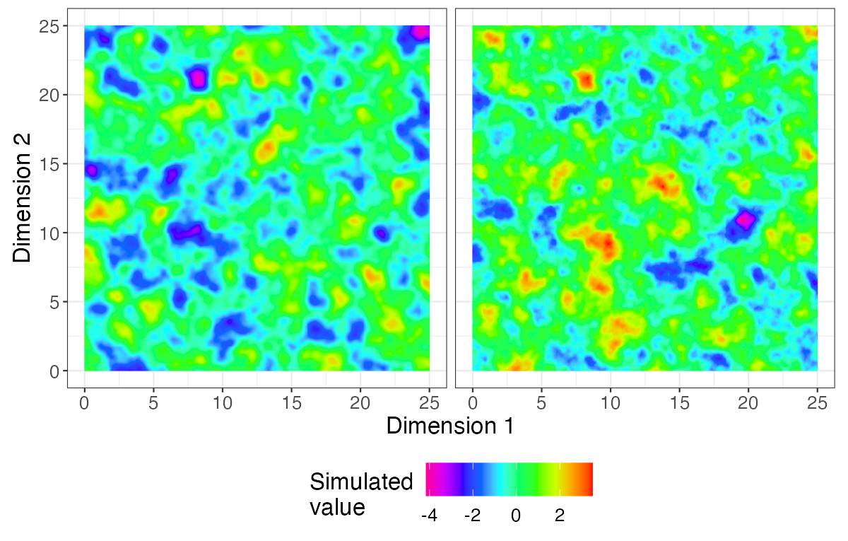
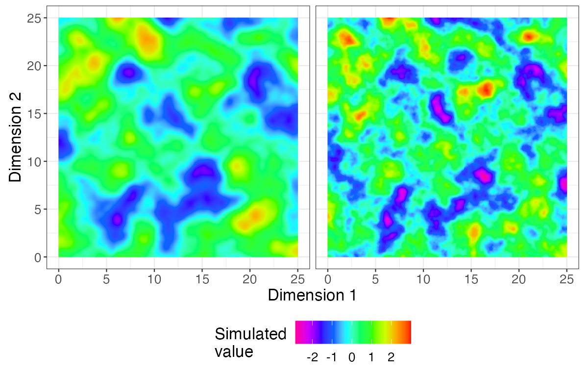
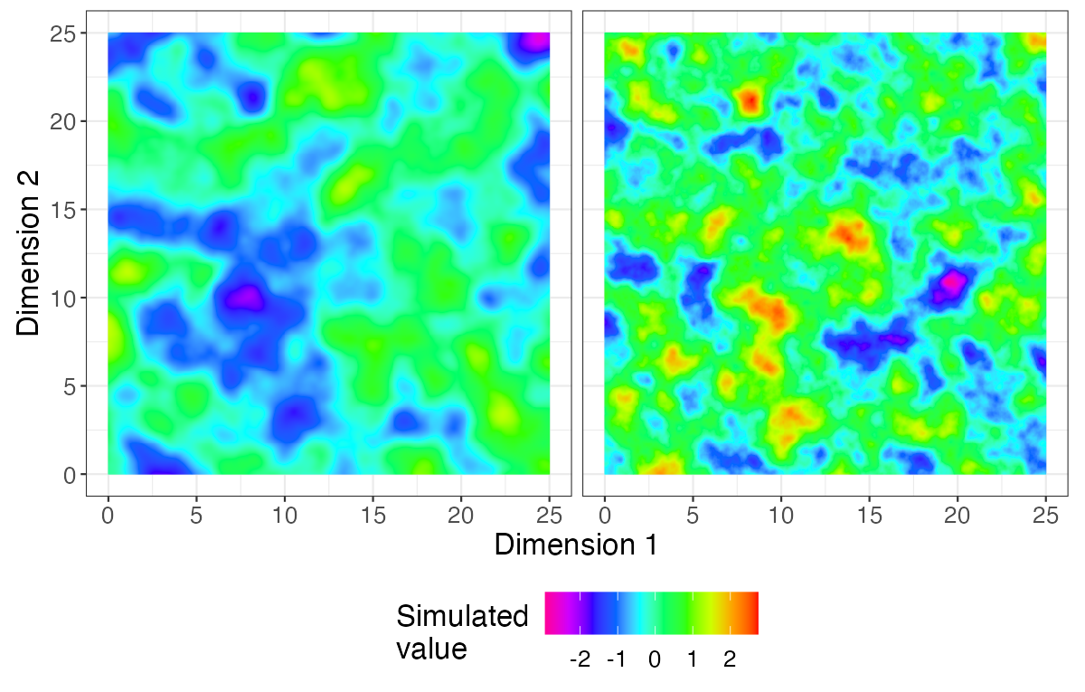
Figure 2: (Top) Bivariate CH processes with $\nu_{1}=2.5$, $\nu_{2}=1.5$, $\alpha_{1}=3$, $\alpha_{2}=1.5$, $\beta_{j}=\beta_{k}=1$, and $\sigma_{jj}=\sigma_{kk}=1$. (Left) With $\sigma_{jk}=0.8$; (Right) With $\sigma_{jk}=-0.8$. (Bottom) Bivariate Matérn processes with $\phi_{jk}=\phi_{jj}=\phi_{kk}=1$, $\nu_{1}=2.5$, $\nu_{2}=1.5$, $\nu_{12}=2$, $\sigma_{jk}=\pm 0.8$.

Using the spectral density of the CH class, we can straightfowardly simulate processes efficiently using the approach of Emery et al., (2016). We plot two simulations of bivariate processes in Figure 2 and compare to simulated bivariate Matérn processes using the same random seed. Similar to results in Ma and Bhadra, (2022), some visual properties of the fields are not very intuitive. For fixed range parameters $\beta_{jk}=\phi_{jk}=1$, the CH covariance decays faster near $h=0$ compared to the Matérn covariance, leading to nearby contrasting values of $Y_{j}(s)$. In addition, as in Ma and Bhadra, (2022), the influence of $\nu_{j}$ is less visually apparent for CH processes compared to the Matérn processes.

3.2 Other validity conditions for the multivariate CH model

We focus on the model in Theorem 3.1 since it gives full flexibility to the parameters of the marginal processes while only slightly increasing the number of parameters needed to estimate the model (principally, the off-diagonal $\sigma_{jk}$ which describe the marginal covariance between processes). We believe that in most cases it would be a suitable model. However, in the multivariate Matérn literature, considerable research has been focused on finding more flexible conditions for validity (Apanasovich et al.,, 2012; Emery et al.,, 2022). For example, we might be interested to have $\nu_{jk}\neq(\nu_{j}+\nu_{k})/2$. We outline additional results here, beginning with the most general setting we consider in this work.

Theorem 3.2.

Consider a multivariate CH covariance of the form $\mathcal{CH}(h;\boldsymbol{\nu},\boldsymbol{\alpha},\boldsymbol{\beta},\boldsymbol{\sigma})$, and note the definition of a conditionally negative semidefinite matrix reviewed in Section S.1 and Emery et al., (2022). If the following conditions hold, then the multivariate CH model is valid:

1. $\boldsymbol{\nu}$ is conditionally negative semidefinite.

2. $\boldsymbol{\beta}$ is conditionally negative semidefinite.

3. $\alpha_{jk}=(\alpha_{jj}+\alpha_{kk})/2$ for all $j$ and $k$.

4. $\frac{\boldsymbol{\sigma}}{\Gamma(\boldsymbol{\nu})\Gamma(\boldsymbol{\alpha})}\boldsymbol{\nu}^{\boldsymbol{\nu}+\frac{d}{2}}{\textrm{exp}}(-\boldsymbol{\nu})\boldsymbol{\beta}^{2\boldsymbol{\alpha}}$ is positive semidefinite.

This extends constructions in Emery et al., (2022); a proof is provided in Section S.1.2.

We next present a theorem that, when some simplifications of the model are made, accomplishes two goals. First, the conditions for validity can be made weaker in some cases, allowing for higher correlation between processes compared to the conditions presented in Theorem 3.1. Second, we may choose $\alpha_{jk}$ more flexibly: $\alpha_{jk}\geq(\alpha_{j}+\alpha_{k})/2>d/2$.

Proposition 3.3.

Consider a multivariate CH covariance of the form $\mathcal{CH}(h;\boldsymbol{\nu},\boldsymbol{\alpha},\boldsymbol{\beta},\boldsymbol{\sigma})$ with the restrictions $\nu_{jk}=(\nu_{j}+\nu_{k})/2$ for all $j$ and $k$, $\alpha_{j}>d/2$ for all $j$, $\alpha_{jk}\geq(\alpha_{j}+\alpha_{k})/2$ for $j\neq k$, and $\beta_{jk}=\beta$ for all $j$ and $k$. This class of models is valid if the matrix $\boldsymbol{\sigma}/B(\boldsymbol{\alpha},\boldsymbol{\nu})$ is positive semidefinite.

The proof is presented in Section S.1.2 and relies on the spectral density of the CH covariance. We next compare Theorem 3.1 and Proposition 3.3 at their intersection: $\alpha_{j}>d/2$, $\alpha_{jk}=(\alpha_{j}+\alpha_{k})/2$, and $\beta_{jk}=\beta$ for all $j$ and $k$. In this setting, Theorem 3.1 establishes that we have the condition of positive semidefiniteness of $\boldsymbol{\sigma}\Gamma(\boldsymbol{\nu}+d/2)/(\Gamma(\boldsymbol{\nu})\Gamma(\boldsymbol{\alpha}))$, while Proposition 3.3 gives the condition of positive semidefiniteness of $\boldsymbol{\sigma}\Gamma(\boldsymbol{\nu}+\boldsymbol{\alpha})/(\Gamma(\boldsymbol{\nu})\Gamma(\boldsymbol{\alpha}))$. Consider the $p=2$ case in $d=1$ with $\alpha_{1}=\nu_{1}=3/2$, $\nu_{12}=(\nu_{1}+\nu_{2})/2$, $\alpha_{12}=(\alpha_{1}+\alpha_{2})/2$, and $\beta_{1}=\beta_{2}=\beta_{12}$. For varying values of $\nu_{2}$ and $\alpha_{2}$, we compute the maximum possible correlation between the processes based on (1) numerical evaluation of the spectral density (2) conditions based on Theorem 3.1, and (3) conditions based on Proposition 3.3.

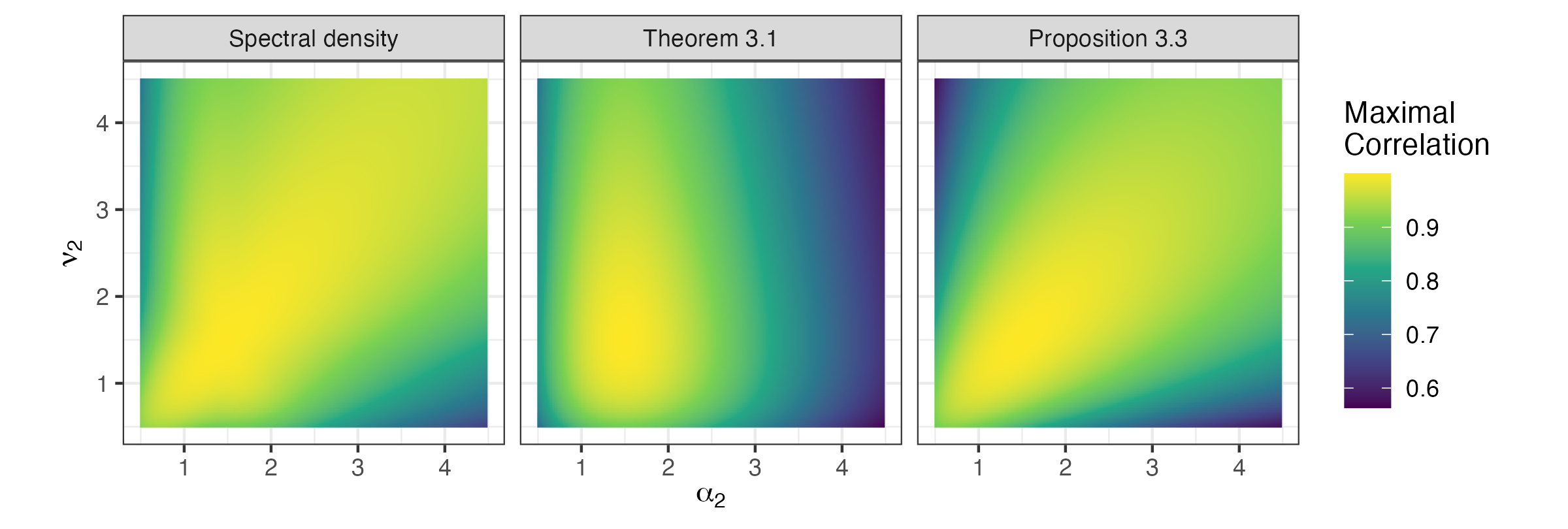
Figure 3: Maximum marginal correlation between two processes with $\nu_{1}=\alpha_{1}=3/2$, $\nu_{12}=(\nu_{1}+\nu_{2})/2$, $\alpha_{12}=(\alpha_{1}+\alpha_{2})/2$, and $\beta_{1}=\beta_{2}=\beta_{12}$. The parameters $\nu_{2}$ and $\alpha_{2}$ are varying. “Spectral density” is based on the spectral density evaluated between $10^{-5}$ to $10^{5}$. The others are based on bounds presented here.

We plot the results in Figure 3. While Theorem 3.1 appears relatively sharp when $|\nu_{2}-\nu_{1}|$ is large and $|\alpha_{2}-\alpha_{1}|$ is small, Proposition 3.3 is sharper when $|\nu_{2}-\nu_{1}|$ is small and $|\alpha_{2}-\alpha_{1}|$ is large. In fact, when $\nu=\nu_{j}=\nu_{k}=\nu_{jk}$, $\alpha_{j}>d/2$, $\alpha_{jk}\geq(\alpha_{j}+\alpha_{k})/2$, and $\beta_{jk}=\beta$ for all $j$ and $k$, the tail behavior of the spectral density in (3) demonstrates that Proposition 3.3 provides a condition that is not only sufficient but also necessary, since the matrix-valued tail of the spectral density decays as $c(x,\nu,\beta,d)\boldsymbol{\sigma}/B(\boldsymbol{\alpha},\boldsymbol{\nu})$ where $c(x,\nu,\beta,d)$ is a positive scalar that does not affect the matrix’s definiteness. In addition, while both Theorems 3.1 and 3.2 assume $\alpha_{jk}=(\alpha_{j}+\alpha_{k})/2$, the additional result in Proposition 3.3 gives more choice in the tail behavior of cross-covariance functions.

We conclude by noting that one cannot construct a valid multivariate CH model when $\nu_{jk}<(\nu_{j}+\nu_{k})/2$, which was also established for the multivariate Matérn in Gneiting et al., (2010). To see this, one may look at the the tail behavior of the matrix-valued spectral density in (3), which cannot be positive semidefinite in this case for arbitrarily large $\lVert x\rVert$.

3.3 Equivalence of Gaussian measures under multivariate CH model

We derive results on the Gaussian equivalence of measures for the multivariate covariance structure, which implies that the multivariate CH class has asymptotically equivalent predictions under different values of the covariance parameters. Let $(\Omega,\mathcal{F})$ be a measurable space with sample space $\Omega$ and $\sigma$-algebra $\mathcal{F}$. Let $\mathcal{P}_{1}(\cdot)$ and $\mathcal{P}_{2}(\cdot)$ be two probability measures on $(\Omega,\mathcal{F})$. We say that $\mathcal{P}_{1}(\cdot)$ and $\mathcal{P}_{2}(\cdot)$ are equivalent on $(\Omega,\mathcal{F})$ if $\mathcal{P}_{1}(\cdot)$ is absolutely continuous with respect to $\mathcal{P}_{2}(\cdot)$ on $(\Omega,\mathcal{F})$ and vice-versa. We say that $\mathcal{P}_{1}(\cdot)$ and $\mathcal{P}_{2}(\cdot)$ are equivalent on the paths of a random process $\boldsymbol{Y}(s)$ if they are equivalent on the $\sigma$-algebra generated by $\boldsymbol{Y}(s)$. Zhang, (2004) has established that the equivalence of Gaussian measures has important implications for parameter estimation. Here, a multivariate random Gaussian process $\boldsymbol{Y}(s)\in\mathbb{R}^{p}$ with mean $(0,0,\dots,0)^{\top}$ and covariance function $\boldsymbol{C}(\cdot;\boldsymbol{\theta})$ on a bounded domain corresponds to a Gaussian measure that we use to evaluate properties of the covariance.

We begin with an equivalence result for the multivariate CH covariance presented in Section 3.1. Similar to Bachoc et al., (2022), we make the following assumption.

Assumption 3.4.

Let $\lambda_{1}(M)$ for a matrix $M$ be the smallest eigenvalue of $M$. Assume that:

$$\inf_{x\geq 0}\lambda_{1}\left(\left[\sigma_{jk}\frac{\Gamma(\nu_{jk}+\frac{d}{2})\beta_{jk}^{d}}{(2\pi)^{\frac{d}{2}}B(\alpha_{jk},\nu_{jk})}\left(1+u\right)^{2\nu+d}\mathcal{U}\left(\nu_{jk}+\frac{d}{2},1-\alpha_{jk}+\frac{d}{2},\beta_{jk}^{2}\frac{u^{2}}{2}\right)\right]_{j,k=1}^{p}\right)>0.$$

This assumption is analogous to Equation 8 of Bachoc et al., (2022), demonstrating that the diagonal elements of the spectral density decay on the order of $(1+u)^{-2\nu-d}$ for large $u$. This also implies that after normalization by $(1+u)^{2\nu+d}$ the matrix spectral density is well-conditioned for any $x\geq 0$. As discussed in Bachoc et al., (2022), such a condition is only slightly more restrictive than ensuring the validity of the multivariate covariance.

Proposition 3.5.

Let $\mathcal{P}_{i}$ be the Gaussian probability measure corresponding to the multivariate covariance $\mathcal{CH}(h;\nu,\boldsymbol{\alpha}^{(i)},\boldsymbol{\beta}^{(i)},\boldsymbol{\sigma}^{(i)})$ for $i=1,2$, $d=1,2,$ or $3$, $\nu>0$, and $\alpha_{jk}^{(i)}>d/2$ for all $j$ and $k$. Assume that Assumption 3.4 holds for both parameter sets $i=1,2$. Then $\mathcal{P}_{1}$ and $\mathcal{P}_{2}$ are equivalent on the paths of $\boldsymbol{Y}(s)$ if:

$$\sigma_{jk}^{(1)}\frac{\Gamma\left(\nu+\alpha_{jk}^{(1)}\right)}{\left(\beta_{jk}^{(1)}\right)^{2\nu}\Gamma\left(\alpha_{jk}^{(1)}\right)}=\sigma_{jk}^{(2)}\frac{\Gamma\left(\nu+\alpha_{jk}^{(2)}\right)}{\left(\beta_{jk}^{(2)}\right)^{2\nu}\Gamma\left(\alpha_{jk}^{(2)}\right)},$$

for all $j$ and $k\in\{1,2,\dots,p\}$.

The proof follows straightforwardly from Theorem 2 of Bachoc et al., (2022) and the characterization of the tail decay of the spectral density in (3). We recover the result presented in Theorem 3 of Ma and Bhadra, (2022) when $p=1$, and for $p>1$ Proposition 3.5 requires checking the condition in Theorem 3 of Ma and Bhadra, (2022) for each of the covariances and cross-covariances. Equivalence results for multivariate processes whose components have different smoothnesses have not been established for the multivariate Matérn model, so we do not consider that extension here. Proposition 3.5 implies that if all processes have the same smoothness parameter $\nu$, the parameters $\beta_{jk}$, $\alpha_{jk}$, and $\sigma_{jk}$ are not identifiable under infill asymptotics on a bounded domain (Zhang,, 2004). Furthermore, it suggests that a misspecified multivariate CH model may attain asymptotically efficient prediction.

We next discuss the equivalence of the multivariate CH covariance and the multivariate Matérn covariance.

Proposition 3.6.

Let $\mathcal{P}_{1}$ be the Gaussian probability measure corresponding to the multivariate covariance $\mathcal{CH}(h;\nu,\boldsymbol{\alpha},\boldsymbol{\beta},\boldsymbol{\sigma}^{(1)})$, $d=1,2,$ or $3$, $\nu>0$, and $\alpha_{jk}>d/2$ for all $j$ and $k$. Assume that Assumption 3.4 holds for these parameters. Let $\mathcal{P}_{\mathcal{M}}$ be the Gaussian probability measure corresponding to the multivariate covariance $\mathcal{M}(h;\nu,\boldsymbol{\phi},\boldsymbol{\sigma}^{(2)})$, $d=1,2,$ or $3$. Assume Equation 8 of Bachoc et al., (2022) holds for this multivariate Matérn covariance. Then $\mathcal{P}_{1}$ and $\mathcal{P}_{\mathcal{M}}$ are equivalent on the paths of $\boldsymbol{Y}(s)$ if:

$$\boldsymbol{\sigma}^{(1)}\frac{2^{\nu}\Gamma\left(\nu+\boldsymbol{\alpha}\right)}{\boldsymbol{\beta}^{2\nu}\Gamma\left(\boldsymbol{\alpha}\right)}=\boldsymbol{\sigma}^{(2)}\frac{1}{\boldsymbol{\phi}^{2\nu}};~{}~{}~{}~{}~{}\textrm{that is, }~{}~{}\sigma_{jk}^{(1)}\frac{2^{\nu}\Gamma\left(\nu+\alpha_{jk}\right)}{\beta_{jk}^{2\nu}\Gamma\left(\alpha_{jk}\right)}=\sigma_{jk}^{(2)}\frac{1}{\phi_{jk}^{2\nu}},$$

for all $j$ and $k\in\{1,2,\dots,p\}$.

This again follows from Theorem 2 of Bachoc et al., (2022) and the spectral densities of the Matérn and CH class. We recover Theorem 4 of Ma and Bhadra, (2022) when $p=1$, and our result essentially implies checking the condition of the result in Ma and Bhadra, (2022) for each of the covariances and cross-covariances.

3.4 Spectrally-generated multivariate CH models

Thus far, we have restricted ourselves to cross-covariances proportional to a CH covariance. However, as discussed by Yarger et al., (2023), Alegría et al., (2021), and Li and Zhang, (2011) among others, cross-covariance functions may have considerably more flexible form. For example, they may be asymmetric so that $\mathbb{E}[Y_{j}(s)Y_{k}(s^{\prime})]\neq\mathbb{E}[Y_{j}(s^{\prime})Y_{k}(s)]$ for $j\neq k$. Yarger et al., (2023) proposed using the spectral density to create more flexible multivariate Matérn models. Since the spectral density of the CH covariance is now available as established in Proposition 2.1, we may follow their approach to construct valid multivariate CH models.

Before introducing asymmetric forms, we first consider an isotropic multivariate covariance using the spectral density with $j$, $k$ entry:

$$\begin{split}&\int_{\mathbb{R}^{d}}e^{\mathbbm{i}h^{\top}x}\sigma_{jk}\left(f_{\mathcal{CH}}(x;\nu_{j},\alpha_{j},\beta_{j},1)\right)^{\frac{1}{2}}\left(f_{\mathcal{CH}}(x;\nu_{k},\alpha_{k},\beta_{k},1)\right)^{\frac{1}{2}}dx.\\ \end{split}$$ (6)

For $j=k$, this reduces to the CH covariance with parameters $\nu_{j}$, $\alpha_{j}$, $\beta_{j}$, and $\sigma_{jj}$; we assume that $\alpha_{j}>d/2$ for all $j$ so that the spectral density is meaningful as a representation of the CH covariance. Since we may represent the matrix-valued spectral density as $\boldsymbol{P}(x)\boldsymbol{\sigma}\boldsymbol{P}(x)^{\top}$ (under matrix multiplication), where $\boldsymbol{P}(x)=\textrm{diag}(f_{\mathcal{CH}}(x;\nu_{j},\alpha_{j},\beta_{j},1)^{\frac{1}{2}},j=1,\dots,p)$, it is evident that the matrix-valued spectral density is positive semidefinite for any $x$ (and thus the model is valid) when $\boldsymbol{\sigma}$ is positive semidefinite. While the integral in (6) likely does not have a closed form, we can compute it efficiently using fast Fourier transforms. This also may be reduced from a $d$-dimensional Fourier transform to a $1$-dimensional Hankel transform based on Stein, (1999):

$$(2\pi)^{\frac{d}{2}}\int_{0}^{\infty}\lVert h\rVert^{-\frac{d-2}{2}}J_{\frac{d-2}{2}}(\lVert h\rVert x)x^{\frac{d}{2}}\sigma_{jk}\left(f_{\mathcal{CH}}(x;\nu_{j},\alpha_{j},\beta_{j},1)\right)^{\frac{1}{2}}\left(f_{\mathcal{CH}}(x;\nu_{k},\alpha_{k},\beta_{k},1)\right)^{\frac{1}{2}}dx.$$ (7)

Like the class of models presented in Theorem 3.1, additional parameters $\nu_{jk}$, $\alpha_{jk}$, and $\beta_{jk}$ for $j\neq k$ do not need to be estimated. In Figure 4, we plot cross-covariances for different parameter values. Predictably, the parameters $\nu_{j}$, $\alpha_{j}$, and $\beta_{j}$ still have influence over the origin behavior, the tail behavior, and the scale of the cross-covariance, respectively.

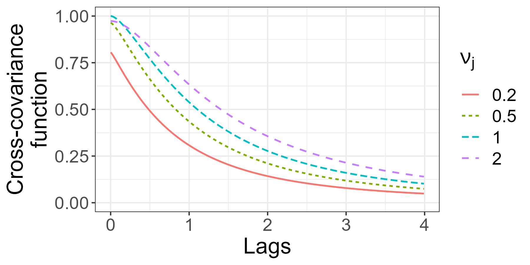
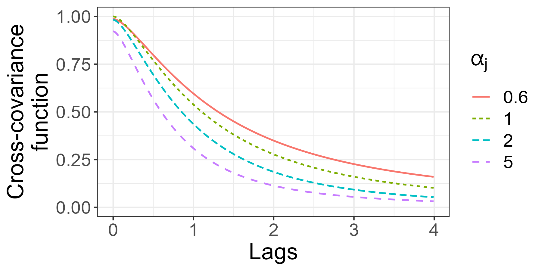
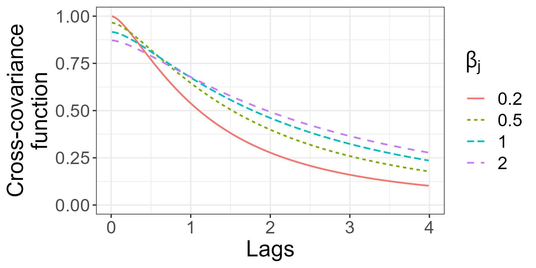
Figure 4: Overview of isotropic spectral cross-covariances in $d=1$ with $\sigma_{jk}=1$. Unless otherwise specified, we take $\nu_{j}=\nu_{k}=\alpha_{j}=\alpha_{k}=\beta_{j}=\beta_{k}=1$ Cross-covariances with $\nu_{j}$ varying (Left), with $\alpha_{j}$ varying (Middle), with $\beta_{j}$ varying (Right).

The approach to create asymmetric forms in the cross-covariance replaces $\sigma_{jk}$ with a complex-valued parameterization. In the setting $d=1$, we consider the multivariate covariance with $j$, $k$ entry:

$$\int_{\mathbb{R}}e^{\mathbbm{i}hx}\left(\Re[\sigma_{jk}]-\textrm{sign}[x]\mathbbm{i}\Im[\sigma_{jk}]\right)\left(f_{\mathcal{CH}}(x;\nu_{j},\alpha_{j},\beta_{j},1)\right)^{\frac{1}{2}}\left(f_{\mathcal{CH}}(x;\nu_{k},\alpha_{k},\beta_{k},1)\right)^{\frac{1}{2}}dx.$$

Here, $\Re[z]$ and $\Im[z]$ denote the real and imaginary parts of $z$, $\textrm{sign}[z]=\mathbb{I}(z>0)-\mathbb{I}(z<0)$ is the sign function, and the matrix of $[\sigma_{jk}]$ is now a positive semidefinite and Hermitian matrix with potentially complex entries on the off-diagonal (continuing to ensure the validity of the model). On the diagonals, $\Im[\sigma_{jj}]=0$ and we return to (6) with a CH covariance. However, on the off-diagonals, if $\Im[\sigma_{jk}]\neq 0$, we obtain asymmetry in the cross-covariance. If $\Re[\sigma_{jk}]=0$, then the cross-covariance is an odd function, that is, $\mathbb{E}[Y_{j}(s)Y_{k}(s^{\prime})]=-\mathbb{E}[Y_{j}(s^{\prime})Y_{k}(s)]$. This follows from the properties of the Hilbert transform of an even function and the relationship between the Hilbert and Fourier transform (King,, 2009); see also the discussion in Section 3.2 of Yarger et al., (2023). In Figure 5, we plot an example of cross-covariances with varying values for $\sigma_{jk}$, with $\nu_{j}=\nu_{k}=1/2$ and $\alpha_{j}=\alpha_{k}=\beta_{j}=\beta_{k}=1$, as well as cross-covariances with $\sigma_{jk}=\mathbbm{i}$ and other parameters varying. By varying $\Re[\sigma_{jk}]$ and $\Im[\sigma_{jk}]$ together, the model’s flexibility covers the symmetric case as well as a variety of asymmetric cases. Similarly to the CH class, the parameters $\alpha_{j}$ and $\alpha_{k}$ appear to control the tail behavior of the cross-covariance, while $\nu_{j}$ and $\nu_{k}$ have more impact near $h=0$.

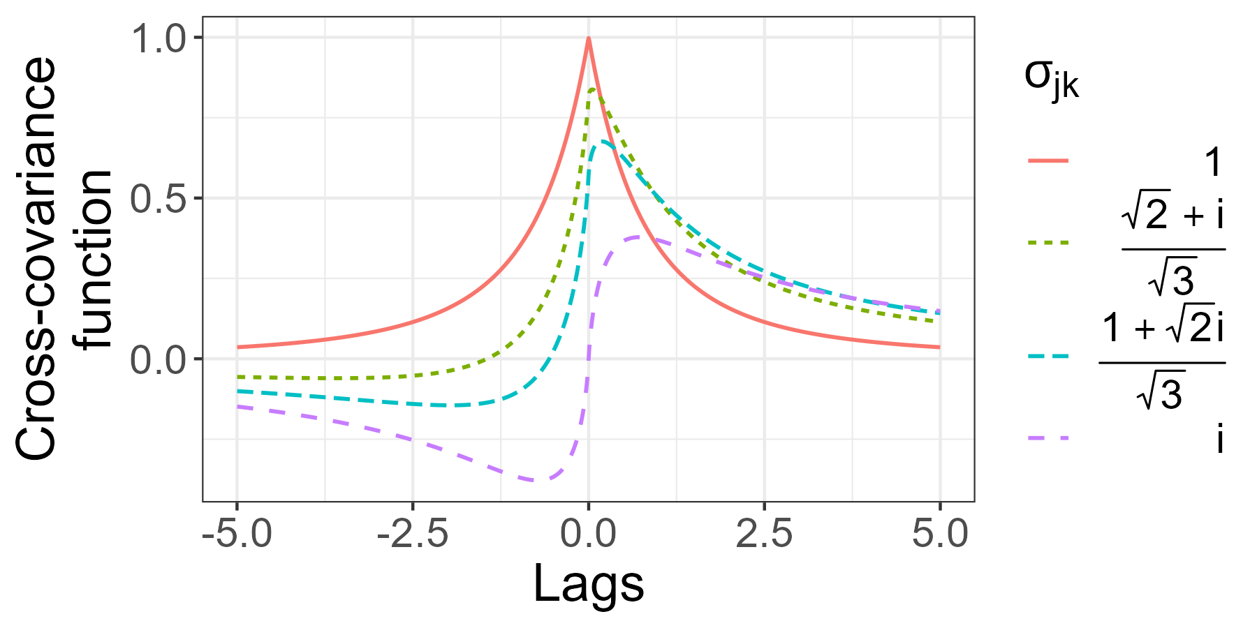
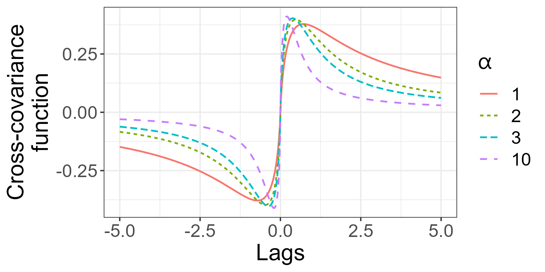
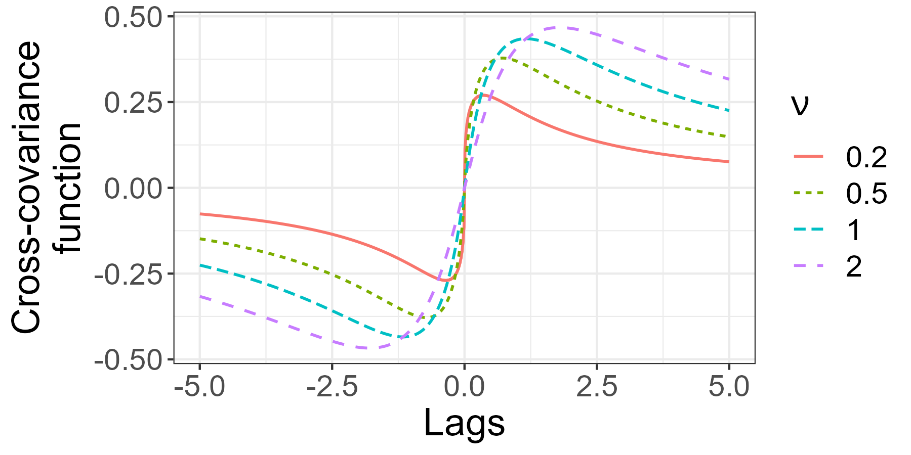
Figure 5: Overview of asymmetric cross-covariances. (Left) Cross-covariances with $\nu_{j}=\nu_{k}=1/2$, $\alpha_{j}=\alpha_{k}=1$, $\beta_{j}=\beta_{k}=1$, and $|\sigma_{jk}|$ held constant, and the real and complex parts of $\sigma_{jk}$ varying. In this setting, $\sigma_{jk}=1$ gives a CH covariance. (Middle and Right) Cross-covariances with $\sigma_{jk}=\mathbbm{i}$ and $\beta_{j}=\beta_{k}=1$: (Middle) varying $\alpha=\alpha_{j}=\alpha_{k}$ with $\nu_{j}=\nu_{k}=1/2$; (Right) varying $\nu=\nu_{j}=\nu_{k}$ with $\alpha_{j}=\alpha_{k}=1$.

For $d>1$, one may extend this model using polar coordinates similar to Section 4 of Yarger et al., (2023). Computations for the spectral approach are more challenging for the multivariate CH covariance compared to the multivariate Matérn covariance in Yarger et al., (2023) due to necessary evaluations of the special functions $\mathcal{U}(\cdot,\cdot,\cdot)$ in the spectral density. While challenging computationally, working through the spectral domain allows for a comprehensive description of the origin behavior of the processes (see Section 6 of Yarger et al.,, 2023).

The spectral approach also enables construction of cross-covariances when it may be unclear what the cross-covariance should be. For example, suppose that $Y_{1}(s)$ has Matérn covariance function $\mathcal{M}(h;\nu_{1},\phi,\sigma_{11})$ and $Y_{2}(s)$ has CH covariance function $\mathcal{CH}(h;\nu_{2},\alpha,\beta,\sigma_{22})$ with $\alpha>d/2$. It is not immediately clear if one can or should use a function proportional to a Matérn covariance or CH covariance as the cross-covariance. However, the cross-covariance generated by $\int_{\mathbb{R}^{d}}e^{\mathbbm{i}h^{\top}x}\sigma_{12}(f_{\mathcal{M}}(x;\nu_{1},\phi,1))^{\frac{1}{2}}(f_{\mathcal{CH}}(x;\nu_{2},\alpha,\beta,1))^{\frac{1}{2}}dx$ for $\sigma_{12}\in\mathbb{R}$ gives a cross-covariance between $Y_{1}(s)$ and $Y_{2}(s)$ that is valid by construction through the spectral density whenever $|\sigma_{12}|\leq\sqrt{\sigma_{11}\sigma_{22}}$. Constructing a cross-covariance between two processes that have a different class of marginal covariance functions was first done (and only done, thus far, to our knowledge) by Porcu et al., (2018).

4 Simulation Experiments

Suppose that we observe samples from a bivariate process consisting of $Y_{1}(s)$ at locations $\boldsymbol{s}_{1}=(s_{11},s_{12},\dots,s_{1n_{1}})$ and $Y_{2}(s)$ at locations $\boldsymbol{s}_{2}=(s_{21},s_{22},\dots,s_{2n_{2}})$. That is, we observe $n_{1}$ samples of $Y_{1}(s)$ and $n_{2}$ samples of $Y_{2}(s)$, with $s_{ji}\in\mathbb{R}^{2}$ for $j\in\{1,2\}$. If $n_{1}=n_{2}$ and $s_{1i}=s_{2i}$ for all $i\in\{1,2,\dots,n_{1}\}$, the processes are observed at the same locations, and we say that our samples of $Y_{1}(s)$ and $Y_{2}(s)$ are colocated. Suppose that we are interested in predicting both $Y_{1}(s)$ and $Y_{2}(s)$ at a set of additional locations $\boldsymbol{s}_{out}$ of size $n_{out}$. For each simulation study, we consider samples of the bivariate process $(Y_{1}(s),Y_{2}(s))$ on the spatial domain of $[0,1]\times[0,1]$. We generate $\boldsymbol{s}_{1}$ as a random sample of points on $[0,1]\times[0,1]$ with $n_{1}=100$. The locations $\boldsymbol{s}_{2}$ are similarly generated with $n_{2}=200$, so that $\boldsymbol{s}_{1}$ and $\boldsymbol{s}_{2}$ are entirely distinct from each other. Finally, we sample $\boldsymbol{s}_{out}$ similarly with $n_{out}=200$, so that we predict at entirely different locations than in $\boldsymbol{s}_{1}$ and $\boldsymbol{s}_{2}$.

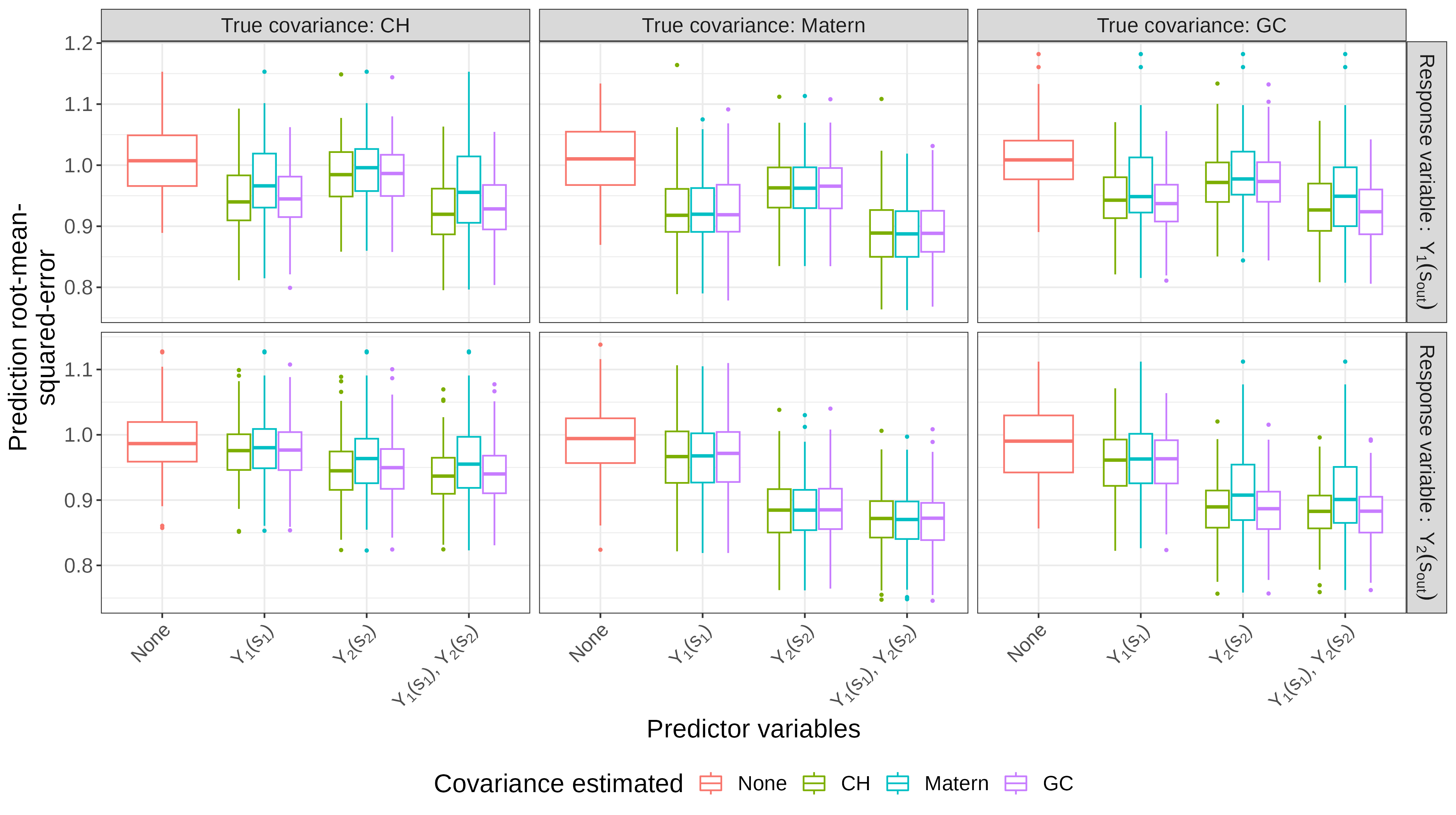
Figure 6: Simulation prediction error results. The boxplots are formed from the prediction RMSE of each of the 100 simulations.

We estimate the parameters numerically by maximum likelihood. For more simple comparison with the Matérn model we assume that one knows that $\beta_{1}=\beta_{2}$. We also consider estimating a bivariate parsimonious Matérn model with $\nu_{12}=(\nu_{1}+\nu_{2})/2$ and $\phi_{12}=\phi_{1}=\phi_{2}$. Finally, as in Ma and Bhadra, (2022), we also estimate a generalized Cauchy (GC) covariance, with multivariate form $\sigma_{jk}\left(1+\left(\frac{\lVert h\rVert}{\phi_{jk}}\right)^{\alpha_{jk}}\right)^{-\frac{\beta_{jk}}{\alpha_{jk}}}.$ Since conditions for validity of the multivariate GC model remain quite technical (see Moreva and Schlather,, 2023; Emery and Porcu,, 2023), we assume that $\alpha_{jk}=\alpha$, $\beta_{jk}=\beta$, and $\phi_{jk}=\phi$ for all $j$ and $k$, which considerably simplifies the estimated covariance. Let $Y_{1}(\boldsymbol{s}_{1})=[Y_{1}(s_{1j})]_{j=1}^{n_{1}}$ and likewise for similar expressions. We consider the predictions using conditional expectations given $Y_{1}(\boldsymbol{s}_{1})$, $Y_{2}(\boldsymbol{s}_{2})$, or both in the Gaussian process setting. We also compare against the null prediction of $0$ at each location. We consider three studies with three different data-generating models; we compare approaches over $100$ simulations, with results presented in Figure 6 and Table 1.

For our first study, we use the multivariate CH covariance with parameters $\nu_{1}=1.75$, $\nu_{2}=1.25$, $\nu_{12}=1.5$, $\alpha_{1}=1.1$, $\alpha_{2}=1.9$, $\alpha_{12}=1.5$, $\beta_{1}=\beta_{2}=\beta_{12}=0.015$, $\sigma_{jj}=\sigma_{kk}=1$, and $\sigma_{jk}=0.60$ and mean zero to generate the data, which results in the conditions of Theorem 3.1 being met. We plot prediction error results in the left column of Figure 6. We see each prediction decreases the error compared to the null prediction. As one expects, using both $Y_{1}(\boldsymbol{s}_{1})$ and $Y_{2}(\boldsymbol{s}_{2})$ gives more accurate predictions compared to using one of them at a time. In general, predictions using the variable that we aim to predict performs better than using only the other variable; however, using only the other variable for prediction still provides substantial improvement over the null prediction of $0$. In this setting where the true multivariate covariance is CH, using the Matérn covariance results in higher prediction error compared to the CH, matching results found in Ma and Bhadra, (2022), while the generalized Cauchy (GC) covariance performs similarly to the CH. In Table 1, we present results from the uncertainty estimates of the predictions based on the conditional variances. In general, the CH and GC intervals tend to be longer and have better calibration to the nominal level of $95\%$ compared to the lagging coverage of intervals when using the Matérn class.

We repeat the simulations when the true multivariate covariance is Matérn with parameters $\phi_{12}=\phi_{11}=\phi_{22}=0.015$, $\sigma_{11}=\sigma_{22}=1$, $\sigma_{12}=0.60$, $\nu_{1}=1.75$, $\nu_{2}=1.25$, and $\nu_{12}=1.50$. We present results in the middle column of Figure 6 and in Table 1. In this setting, the CH, Matérn, and GC multivariate covariances perform essentially the same for point estimation and uncertainty quantification for all versions of the prediction, demonstrating (as in Ma and Bhadra,, 2022) that the CH class performs well even when the true covariance is Matérn.

Finally, we repeat the simulations when the true covariance is generalized Cauchy. In particular, we take $\alpha_{jk}=1$, $\beta_{jk}=1$, and $\phi_{jk}=0.015$ for all $j$ and $k$. The results are presented in the right column of Figure 6 and also in Table 1. The Matérn again performs worse in point prediction and interval coverage compared to the CH and GC classes. The CH and GC covariances perform similarly when GC is the true covariance. In general, while the CH and GC perform similarly in the above simulation setups, the GC has much more complicated expressions for validity (Emery and Porcu,, 2023; Moreva and Schlather,, 2023), making application for processes with different marginal parameters more challenging compared to the multivariate CH covariance introduced in this paper.

	Predictor variables	Response variable	95% CI coverage			Average length
			CH	M	GC	CH	M	GC
True covariance: CH	$Y_{1}(\boldsymbol{s}_{1})$	$Y_{1}(\boldsymbol{s}_{out})$	94.2	83.1	95.1	3.61	2.99	3.73
	$Y_{2}(\boldsymbol{s}_{2})$	$Y_{1}(\boldsymbol{s}_{out})$	94.6	83.4	94.2	3.83	3.12	3.77
	$Y_{1}(\boldsymbol{s}_{1})$, $Y_{2}(\boldsymbol{s}_{2})$	$Y_{1}(\boldsymbol{s}_{out})$	93.9	83.0	94.9	3.51	2.93	3.64
	$Y_{1}(\boldsymbol{s}_{1})$	$Y_{2}(\boldsymbol{s}_{out})$	95.0	83.5	95.3	3.85	3.08	3.90
	$Y_{2}(\boldsymbol{s}_{2})$	$Y_{2}(\boldsymbol{s}_{out})$	94.9	83.3	94.6	3.71	2.99	3.69
	$Y_{1}(\boldsymbol{s}_{1})$, $Y_{2}(\boldsymbol{s}_{2})$	$Y_{2}(\boldsymbol{s}_{out})$	94.7	83.3	94.5	3.66	2.95	3.65
True covariance: Matérn	$Y_{1}(\boldsymbol{s}_{1})$	$Y_{1}(\boldsymbol{s}_{out})$	94.4	94.4	95.0	3.53	3.53	3.61
	$Y_{2}(\boldsymbol{s}_{2})$	$Y_{1}(\boldsymbol{s}_{out})$	94.5	94.5	94.3	3.74	3.74	3.71
	$Y_{1}(\boldsymbol{s}_{1})$, $Y_{2}(\boldsymbol{s}_{2})$	$Y_{1}(\boldsymbol{s}_{out})$	94.2	94.1	94.8	3.37	3.37	3.45
	$Y_{1}(\boldsymbol{s}_{1})$	$Y_{2}(\boldsymbol{s}_{out})$	94.9	94.9	95.1	3.80	3.80	3.85
	$Y_{2}(\boldsymbol{s}_{2})$	$Y_{2}(\boldsymbol{s}_{out})$	94.8	94.7	94.7	3.43	3.43	3.43
	$Y_{1}(\boldsymbol{s}_{1})$, $Y_{2}(\boldsymbol{s}_{2})$	$Y_{2}(\boldsymbol{s}_{out})$	94.7	94.6	94.6	3.36	3.35	3.36
True covariance: GC	$Y_{1}(\boldsymbol{s}_{1})$	$Y_{1}(\boldsymbol{s}_{out})$	94.1	86.4	94.6	3.63	3.15	3.65
	$Y_{2}(\boldsymbol{s}_{2})$	$Y_{1}(\boldsymbol{s}_{out})$	94.6	86.4	94.5	3.78	3.24	3.77
	$Y_{1}(\boldsymbol{s}_{1})$, $Y_{2}(\boldsymbol{s}_{2})$	$Y_{1}(\boldsymbol{s}_{out})$	93.7	86.2	94.5	3.54	3.08	3.57
	$Y_{1}(\boldsymbol{s}_{1})$	$Y_{2}(\boldsymbol{s}_{out})$	95.1	86.9	95.2	3.79	3.24	3.80
	$Y_{2}(\boldsymbol{s}_{2})$	$Y_{2}(\boldsymbol{s}_{out})$	94.9	86.6	95.0	3.50	3.02	3.49
	$Y_{1}(\boldsymbol{s}_{1})$, $Y_{2}(\boldsymbol{s}_{2})$	$Y_{2}(\boldsymbol{s}_{out})$	94.7	86.5	94.8	3.46	2.99	3.46

Table 1: Prediction interval summaries under different true covariances. We compare estimated CH, Matérn (M), and generalized Cauchy (GC) multivariate covariances.

In Section S.2, we provide additional simulations that may interest the reader, including results for predictions using $Y_{2}(\boldsymbol{s}_{out})$ when we aim to predict $Y_{1}(\boldsymbol{s}_{out})$ and vice versa, a colocated simulation design, and estimation of the isotropic spectrally-generated multivariate CH model proposed in (7).

5 Analysis of Oceanography Data

For data analysis, we consider an oceanography dataset of temperature, salinity, and oxygen from the Southern Ocean Carbon and Climate Observations and Modeling (SOCCOM) project (Johnson et al.,, 2020), consisting of measurements of these variables at different depths in the ocean collected by autonomous devices called floats. The SOCCOM project is part of the larger Argo project dedicated to float-based monitoring of the oceans (Wong et al.,, 2020; Argo,, 2023). Most Argo floats collect only temperature and salinity data; we refer to them as Core Argo floats. However, some floats also collect BioGeoChemical (BGC) variables including oxygen, pH and nitrate; we refer to these as BGC Argo floats. The multivariate relationship of temperature, salinity, and oxygen can inform how one uses available Core Argo data to predict biogeochemical variables like oxygen. The problem of estimating oxygen based on temperature and salinity data has received interest in Giglio et al., (2018) and Korte-Stapff et al., (2022). We focus on an area in the Southern Ocean bounded by 100 and 180 degrees of longitude from a depth of 150m in the ocean. We include data from the months of February, March, and April over the years 2017-2023, resulting in 436 total locations. We plot salinity and temperature data from SOCCOM BGC floats in Figure 1.

5.1 Model estimation

Based on the original data in Figure 1, we see that the mean of the data depends on longitude and latitude, and thus we estimate a spatially varying mean using local regression. In particular, we use local linear smoothing in terms of longitude and latitude with a bandwidth of 1,000 kilometers. The mean is subtracted from the original data and the resulting residuals are presented in Figure1 also and used in our covariance analysis. We treat the residuals in a similar way to Kuusela and Stein, (2018)—locally stationary, so that we estimate a stationary model for the residuals in this region, and we assume data from different years are independent, so that the overall log-likelihood is the sum of the log-likelihoods from each of the seven years. We estimate isotropic trivariate CH and Matérn covariances of the form from Section 3.1, with the addition of a nugget variance parameter $\tau$ (that is, we assume our data has additional noise normally distributed with variance $\tau$) for each of the three processes, which was also done in previous analysis in the literature (for example, Gneiting et al.,, 2010; Kuusela and Stein,, 2018).

Parameter	CH Estimate	M Estimate	Parameter	CH Estimate	M Estimate
$\nu_{S}$	0.388	0.376	$\sigma_{S}$	0.0257	0.0251
$\nu_{O}$	0.154	0.158	$\sigma_{O}$	92.327	91.708
$\nu_{T}$	0.432	0.432	$\sigma_{T}$	1.584	1.670
$\alpha_{S}$	0.768	-	$\sigma_{SO}/\sqrt{\sigma_{S}\sigma_{O}}$	-0.705	-0.691
$\alpha_{O}$	0.475	-	$\sigma_{ST}/\sqrt{\sigma_{S}\sigma_{T}}$	0.700	0.741
$\alpha_{T}$	2.700	-	$\sigma_{TO}/\sqrt{\sigma_{T}\sigma_{O}}$	-0.543	-0.559
$\beta_{S}$ or $\phi_{S}$	472.7	506.2	$\tau_{S}/\sigma_{S}$	0.0577	0.0461
$\beta_{O}$ or $\phi_{O}$	584.5	769.0	$\tau_{O}/\sigma_{O}$	0.0003	0.0001
$\beta_{T}$ or $\phi_{T}$	721.6	442.8	$\tau_{T}/\sigma_{T}$	0.0021	0.0005

Table 2: Estimated parameters for the CH and Matérn (M) models for the Argo data. The subscripts S, O, and T represent salinity, oxygen, and temperature, respectively.

Since the locations are colocated, we compute marginal correlation estimates between the processes before estimation by maximum likelihood. Temperature and salinity had a correlation coefficient of $0.694$, temperature and oxygen had a coefficient of $-0.551$, and salinity and oxygen had a coefficient of $-0.690$. We present the parameter estimates resulting from maximum likelihood estimation in Table 2. For the most part, the parameters that the two covariances share have similar estimates, including the marginal variances, covariances, smoothnesses, and nugget effects. For salinity and oxygen, the CH covariance estimates relatively heavy tails for the covariance functions with smaller values for $\alpha_{S}$ and $\alpha_{O}$.

5.2 Prediction

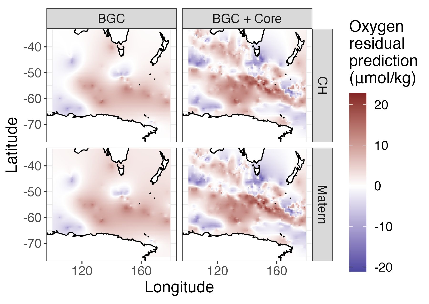
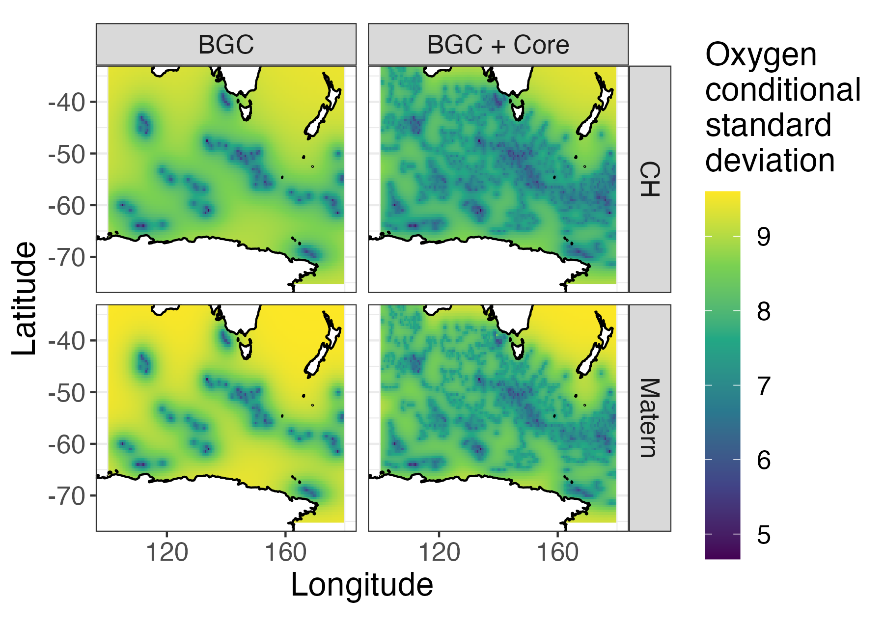
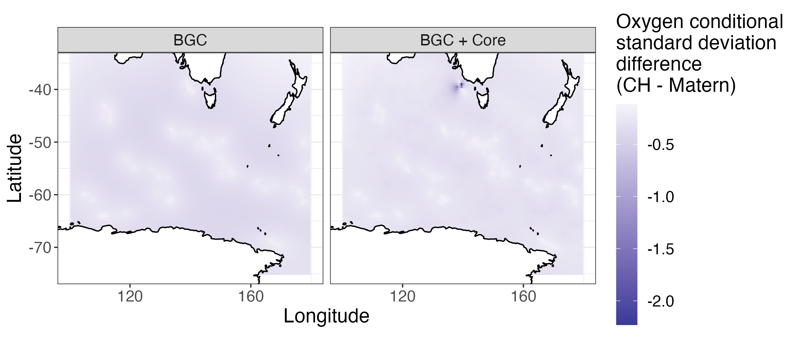
Figure 7: (Top Left) Prediction of oxygen in 2019 based on CH and Matérn multivariate covariances. (Top Right) Conditional standard deviations of oxygen in 2019. (Bottom) Difference of conditional standard deviations of the CH and Matérn multivariate covariances.

We use our estimated covariance functions to predict oxygen, temperature, and salinity on a regular $1/2$ degree grid in this area, and present results from oxygen here. As in the simulation studies, we use the conditional expectation and variance to provide predictions and uncertainties on this grid. In addition to the 436 profiles used in the training of the data, we also use 8,264 additional nearby Argo Core profiles that only have temperature and salinity data. Ideally, the much more abundant Core data can provide improved information about oxygen using the estimated covariance between the variables. For each year, we form a prediction with and without these additional Core data. In the top left panel of Figure 7, we plot the predictions for 2019. We see that the CH and Matérn covariances give similar predictions, and including Core data increases the granularity of the predictions.

On the top right panel of Figure 7, we plot the corresponding conditional standard deviations. In general, we see that the CH standard deviations appear smaller than the Matérn ones, especially further away from any observed location. This matches results found in the univariate case in Ma and Bhadra, (2022). When using Core data, we also see that the additional Core profiles considerably decrease the prediction standard deviations. On the other hand, the areas with the lowest standard deviations are near locations where BGC data was collected. In the bottom panel of Figure 7, we plot the difference in conditional variances, again confirming that the CH covariance gives generally smaller conditional variances compared to the Matérn covariance function. As the BGC Argo expands to a global array (Matsumoto et al.,, 2022), providing predictions and uncertainty estimates for both data-sparse and data-dense settings will be useful.

To further evaluate performance, we estimate prediction error using cross-validation. We consider two-fold cross-validation by float, which represents a data-sparse situation, as well as leave-one-float-out cross-validation. Similarly to the prediction above, we also use predictions from BGC only as well as BGC and Core data. Results are summarized in Table 3. As expected, prediction errors for both the CH and Matérn covariance functions were less when using additional Core Argo data. In 2-fold cross-validation, the CH multivariate covariance performs similarly to the multivariate Matérn when using Core data, but generally performs better than the Matérn when using BGC data only. This reflects that the CH covariance will be most useful in data-sparse settings where the tails of the covariance function will have more influence. In the leave-float-out setting, the CH and Matérn covariances perform similarly when using BGC data only, while when using the BGC + Core data (representing the most data-dense setting of the four we consider here), the Matérn covariance performs slightly better than the CH covariance. Throughout the settings, the CH multivariate covariance provides generally shorter prediction intervals with comparable coverage to the Matérn. In these settings, the use of the multivariate CH covariance compared to the multivariate Matérn appears to affect the uncertainty estimates more than the point prediction performance.

	2-fold				Leave-float-out
Prediction	RMSE	MAE	Cov	I Len	RMSE	MAE	Cov	I Len
CH, BGC	9.08	6.50	94.7	9.08	8.97	6.30	94.5	8.65
Matérn, BGC	9.40	6.45	94.9	9.43	8.93	6.33	95.4	8.99
CH, BGC + core	7.03	4.20	92.7	6.53	7.03	4.26	92.7	6.34
Matérn, BGC + core	6.93	4.18	94.0	6.78	6.94	4.23	93.6	6.69

Table 3: Oxygen prediction results, for root-mean-squared-error (RMSE), median absolute error (MAE), coverage of 95% confidence intervals (Cov), and median interval length (I Len).

6 Discussion

In this work, we study multivariate generalizations of the Confluent Hypergeometric covariance, proposed by Ma and Bhadra, (2022), that has polynomial-decaying tail behavior, while preserving the flexible origin behavior of Matérn. We focus on the case where the cross-covariances are proportional to a Confluent Hypergeometric covariance. We establish general conditions for the validity of this model, including instances when the marginal covariances have different smoothnesses or origin behavior, different tail behavior, and different range parameters, thus allowing full flexibility to the marginal covariances while modeling dependence between the processes. We also provide more flexible conditions for validity. Properties of this cross-covariance, including its tail decay and spectral density, are readily available, and we also give conditions for the equivalence of measures for the multivariate model. These results establish that parameters of the multivariate model are not jointly identifiable, but one may obtain asymptotically optimal predictions using a misspecified model. In simulations, we demonstrate that the proposed class performs better (in terms of prediction error and uncertainty quantification) than the multivariate Matérn class when the true covariance is CH, and that when the true covariance is Matérn, they perform similarly. The proposed cross-covariances are used to predict oceanographic oxygen levels from temperature and salinity in the Southern Ocean. We find that the multivariate CH covariance results in lower estimated predicted variances; in a data-sparse cross-validation experiment, the multivariate CH performs better compared to the multivariate Matérn in data-sparse situation, while they perform similarly otherwise.

Also newly established in this work is the spectral density of the Confluent Hypergeometric covariance. This provides a more precise description of the multivariate model and conditions for its validity. It also enables us to construct multivariate models that are spectrally-generated in a manner similar to the approach recently proposed in Yarger et al., (2023). These models are immediately valid by construction, and we use this approach to introduce more flexible asymmetric cross-covariances. We also straightforwardly propose a cross-covariance between a process with a Matérn covariance function and a process with a Confluent Hypergeometric covariance function.

We outline some areas for future work. Extensions of the work here could include space-time models (cf. Porcu et al.,, 2021; Chen et al.,, 2021) and nonstationary models (similarly to, for example, Kleiber and Nychka,, 2012). Such extensions are relavant for a more sophisticated analysis to the Argo data (Kuusela and Stein,, 2018). One property of the multivariate covariance we have not explored in detail here is coherence (Kleiber,, 2017). Due to the at-times opaque nature of the spectral density through its dependence on $\mathcal{U}(\nu+d/2,1-\alpha+d/2,\cdot)$, interpretable and detailed expressions of the coherence will be more challenging to access compared to the multivariate Matérn covariance. However, numerical study suggests that, like for the multivariate Matérn, the squared coherence may peak at $x\to 0$, $0<x<\infty$, or $x\to\infty$. As with other multivariate covariances, considering highly-multivariate processes may make application of this model possible in more settings, similar to the problems considered by Dey et al., (2022) and Krock et al., (2023).

7 Acknowledgements

Data were collected and made freely available by the Southern Ocean Carbon and Climate Observations and Modeling (SOCCOM) Project funded by the National Science Foundation, Division of Polar Programs (NSF PLR-1425989 and OPP-1936222), supplemented by NASA, and by the International Argo Program and the NOAA programs that contribute to it. (http://www.argo.ucsd.edu, https://www.ocean-ops.org/board). The Argo Program is part of the Global Ocean Observing System.

SUPPLEMENTARY MATERIAL

(a) Supplementary Text: contains proofs, additional results from simulations, and additional plots from the data analysis.
(b) Supplementary Code: contains computer code archive along with a README file: https://github.com/dyarger/multivariate_confluent_hypergeometric.

Supplementary Material to
On Valid Multivariate Generalizations of the Confluent Hypergeometric Covariance Function

S.1 Definitions and Proofs

S.1.1 Conditionally negative semidefinite matrices

Definition S.1.1.

A $p\times p$ matrix $\boldsymbol{A}=[a_{jk}]$ is said to be conditionally negative semidefinite, if, for any $p$-vector $x=(x_{1},\dots,x_{p})^{\top}$ such that $\sum_{j=1}^{p}x_{j}=0$, then:

$$x^{\top}\boldsymbol{A}x =\sum_{j=1}^{p}\sum_{k=1}^{p}x_{j}x_{k}a_{jk}\leq 0.$$

See Emery et al., (2022) for discussion and references relating to this definition, which they use to show validity conditions for the multivariate Matérn model.

Throughout the remainder of Section S.1, let $\boldsymbol{\nu}$, $\boldsymbol{\alpha}$, $\boldsymbol{\beta}$, and $\boldsymbol{\sigma}$ be matrices of parameters, and take all matrix operations elementwise. In the following, we will most essentially use the relationship that $\textrm{exp}\left(-t\boldsymbol{A}\right)\textrm{ is positive semidefinite for all }t>0$ if and only if $\boldsymbol{A}\textrm{ is conditionally negative semidefinite}$ (Berg et al.,, 1984; Emery et al.,, 2022).

S.1.2 Proofs

We first discuss the general necessary and sufficient condition for validity when all $\alpha_{jk}>d/2$ using the spectral density. This will be used in some of the later proofs.

Proposition S.1.2.

Consider a multivariate covariance on $\mathbb{R}^{d}$ defined by $\mathcal{CH}(h;\boldsymbol{\nu},\boldsymbol{\alpha},\boldsymbol{\beta},\boldsymbol{\sigma})$. Suppose that $\alpha_{jk}>d/2$ for all $j$ and $k$. Then the multivariate model is valid if and only if:

$$\boldsymbol{\sigma}\frac{\Gamma(\boldsymbol{\nu}+\frac{d}{2})\boldsymbol{\beta}^{d}}{B(\boldsymbol{\alpha},\boldsymbol{\nu})}\mathcal{U}\left(\boldsymbol{\nu}+\frac{d}{2},1-\boldsymbol{\alpha}+\frac{d}{2},\boldsymbol{\beta}^{2}\frac{u}{2}\right),$$

is positive semidefinite for all $u>0$.

Proof.

This follows from checking that the matrix-valued spectral density is positive semidefinite for all of its inputs. ∎

Since the function $\mathcal{U}(\cdot,\cdot,\cdot)$ is relatively opaque, finding more simple necessary and sufficient conditions is likely not possible. However, for specific values of some parameters, like in Proposition 3.3, this relationship may be used to establish valid models.

We now discuss the proofs in order of presentation in the main paper.

Proof of Proposition 2.1.

Throughout, we use the shorthand of $f_{\mathcal{CH}}(x)=f_{\mathcal{CH}}(x;\nu,\alpha,\beta,\sigma^{2})$. Since the covariance only depends on $h$ through its length $\lVert h\rVert$, one may use the inversion-type formulas on page 46 of Stein, (1999) when $\alpha>d/2$:

$$f_{\mathcal{CH}}(x) =(2\pi)^{-\frac{d}{2}}\int_{0}^{\infty}(w\lVert x\rVert)^{-\frac{d-2}{2}}J_{\frac{d-2}{2}}(w\lVert x\rVert)w^{d-1}\mathcal{CH}(w;\nu,\alpha,\beta,\sigma^{2})dw$$

$$=\sigma^{2}\frac{\Gamma(\nu+\alpha)}{\Gamma(\nu)(2\pi)^{\frac{d}{2}}}\lVert x\rVert^{-\frac{d-2}{2}}\int_{0}^{\infty}J_{\frac{d-2}{2}}(w\lVert x\rVert)w^{\frac{d}{2}}\mathcal{U}\left(\alpha,1-\nu,\frac{w^{2}}{2\beta^{2}}\right)dw.$$

Consider the change of variables $u=w^{2}/(2\beta^{2})$ with $dw=\beta/\sqrt{2u}du$, so that

$$f_{\mathcal{CH}}(x) =\sigma^{2}\frac{\Gamma(\nu+\alpha)}{\Gamma(\nu)(2\pi)^{\frac{d}{2}}}\lVert x\rVert^{-\frac{d-2}{2}}2^{\frac{d}{4}-\frac{1}{2}}\beta^{\frac{d}{2}+1}\int_{0}^{\infty}u^{\frac{d}{4}-\frac{1}{2}}\mathcal{U}\left(\alpha,1-\nu,u\right)J_{\frac{d-2}{2}}\left(\beta\sqrt{2u}\lVert x\rVert\right)du.$$

We now apply 13.10.15 of DLMF, (2021), which states

$$\int_{0}^{\infty}u^{\frac{\mu}{2}}\mathcal{U}(a,b,u)J_{\mu}(2\sqrt{yu})dt=\frac{\Gamma(\mu-b+2)}{\Gamma(a)}y^{\frac{1}{2}\mu}\mathcal{U}(\mu-b+2,\mu-a+2,y).$$

If we set $\mu=(d-2)/2$, $a=\alpha$, $b=1-\nu$, and $y=\beta^{2}\lVert x\rVert^{2}/2$, the restrictions given in 13.10.15 of DLMF, (2021) are satisfied, and we have

$$f_{\mathcal{CH}}(x) =\sigma^{2}\frac{\Gamma(\nu+\alpha)}{\Gamma(\nu)(2\pi)^{\frac{d}{2}}}\lVert x\rVert^{-\frac{d-2}{2}}2^{\frac{d}{4}-\frac{1}{2}}\beta^{\frac{d}{2}+1}\frac{\Gamma(\nu+\frac{d}{2})}{\Gamma(\alpha)}\left(\frac{\beta\lVert x\rVert}{\sqrt{2}}\right)^{\frac{d-2}{2}}\mathcal{U}\left(\nu+\frac{d}{2},1-\alpha+\frac{d}{2},\frac{\beta^{2}\lVert x\rVert^{2}}{2}\right)$$

$$=\sigma^{2}\frac{\Gamma(\nu+\frac{d}{2})\beta^{d}}{B(\nu,\alpha)(2\pi)^{\frac{d}{2}}}\mathcal{U}\left(\nu+\frac{d}{2},1-\alpha+\frac{d}{2},\frac{\beta^{2}\lVert x\rVert^{2}}{2}\right).$$

The proof of this result may also be shown (more tediously) using Relation 14.4(13) of Bateman, (1954). ∎

Proof of Theorem 3.2.

The general approach for construction of this model is to combine Example 2 of Emery et al., (2022) with mixing with respect to a matrix composed of inverse-gamma densities. In Emery et al., (2022), they establish that the multivariate Matérn model:

$$\boldsymbol{\sigma}\left(\frac{|h|}{\phi}\right)^{\boldsymbol{\nu}}\mathcal{K}_{\boldsymbol{\nu}}\left(\frac{|h|}{\phi}\right),$$

is valid if $\boldsymbol{\nu}$ is conditionally negative semidefinite and $\boldsymbol{\sigma}\Gamma(\boldsymbol{\nu})^{-1}\boldsymbol{\nu}^{\nu+\frac{d}{2}}\textrm{exp}(-\boldsymbol{\nu})$ is positive semidefinite. We consider the mixture:

$$\int_{0}^{\infty}\boldsymbol{\sigma}\left(\frac{|h|}{\phi}\right)^{\boldsymbol{\nu}}\mathcal{K}_{\boldsymbol{\nu}}\left(\frac{|h|}{\phi}\right)\frac{\boldsymbol{\beta}^{2\boldsymbol{\alpha}}}{2^{\boldsymbol{\alpha}}\Gamma(\boldsymbol{\alpha})}\phi^{-2\boldsymbol{\alpha}-2}\textrm{exp}\left(-\frac{\boldsymbol{\beta}^{2}}{2\phi^{2}}\right)d\phi^{2}.$$

We are interested when the integrand is positive semidefinite for any $\phi^{2}>0$. Due to the choice of $\boldsymbol{\alpha}$, $\phi^{-2\boldsymbol{\alpha}-2}2^{-\boldsymbol{\alpha}}$ can be removed due to the Schur product theorem or by left and right multiplication by the diagonal matrix of $2^{\alpha_{j}/2}\phi^{\alpha_{j}-1}$ for $j=1,\dots,p$. We are then left to check that $\boldsymbol{\nu}$ is conditionally negative semidefinite, and,

$$\frac{\boldsymbol{\sigma}}{\Gamma(\boldsymbol{\nu})}\boldsymbol{\nu}^{\nu+\frac{d}{2}}\textrm{exp}(-\boldsymbol{\nu})\frac{\boldsymbol{\beta}^{2\boldsymbol{\alpha}}}{\Gamma(\boldsymbol{\alpha})}\textrm{exp}\left(-\frac{\boldsymbol{\beta}^{2}}{2\phi^{2}}\right),$$

is positive semidefinite for any $\phi>0$. Under the assumption that $\boldsymbol{\beta}$ is conditionally negative semidefinite, the matrix $\textrm{exp}(-\boldsymbol{\beta}^{2}/(2\phi^{2}))$ is positive semidefinite for all $\phi^{2}>0$. By the Schur product theorem, the conditions imply that the multivariate model is valid. ∎

Proof of Proposition 3.3.

We consider the conditions under which the matrix of

$$f_{\mathcal{CH}}\left(x;\frac{\nu_{j}+\nu_{k}}{2},\alpha_{jk},\beta,\sigma_{jk}\right),$$

is positive semidefinite for all $x$. That is, we examine the matrix of:

$$\sigma_{jk}\frac{\Gamma(\frac{\nu_{j}+\nu_{k}}{2}+\frac{d}{2})\beta^{d}}{(2\pi)^{d/2}B(\alpha_{jk},\frac{\nu_{j}+\nu_{k}}{2})}\mathcal{U}\left(\frac{\nu_{j}+\nu_{k}}{2}+\frac{d}{2},1-\alpha_{jk}+\frac{d}{2},\frac{\beta^{2}\lVert x\rVert^{2}}{2}\right).$$

By left and right multiplying by the matrix:

$$\textrm{diag}\left(\frac{(2\pi)^{\frac{d}{4}}}{\beta^{\frac{d}{2}}\sqrt{\Gamma(\nu_{j}+\frac{d}{2})\mathcal{U}\left(\nu_{j}+\frac{d}{2},1-\alpha_{j}+\frac{d}{2},\frac{\beta^{2}\lVert x\rVert^{2}}{2}\right)}},j=1,\dots,p\right),$$

we see that this is equivalent to the checking the positive semidefiniteness of the matrix:

$$\sigma_{jk}\begin{cases}\frac{1}{B(\alpha_{j},\nu_{j})},&j=k,\\ \frac{1}{B(\alpha_{jk},\frac{\nu_{j}+\nu_{k}}{2})}\frac{\Gamma(\frac{\nu_{j}+\nu_{k}}{2}+\frac{d}{2})\mathcal{U}\left(\frac{\nu_{j}+\nu_{k}}{2}+\frac{d}{2},1-\alpha_{jk}+\frac{d}{2},\frac{\beta^{2}\lVert x\rVert^{2}}{2}\right)}{\sqrt{\Gamma(\nu_{j}+\frac{d}{2})\mathcal{U}\left(\nu_{j}+\frac{d}{2},1-\alpha_{j}+\frac{d}{2},\frac{\beta^{2}\lVert x\rVert^{2}}{2}\right)\Gamma(\nu_{k}+\frac{d}{2})\mathcal{U}\left(\nu_{k}+\frac{d}{2},1-\alpha_{k}+\frac{d}{2},\frac{\beta^{2}\lVert x\rVert^{2}}{2}\right)}},&j\neq k,\end{cases}$$

for each $x$. Theorem 2.3 of Bhukya et al., (2018) establishes that:

$$|\mathcal{U}(a,c_{1},x)|\leq|\mathcal{U}(a,c,x)|$$

for $c_{1}<c$, $a>0$, $x>0$. Applying this to the cross-spectral density, we have:

$$\left|\mathcal{U}\left(\frac{\nu_{j}+\nu_{k}}{2}+\frac{d}{2},1-\alpha_{jk}+\frac{d}{2},\frac{\beta^{2}\lVert x\rVert^{2}}{2}\right)\right|\leq\left|\mathcal{U}\left(\frac{\nu_{j}+\nu_{k}}{2}+\frac{d}{2},1-\frac{\alpha_{j}+\alpha_{k}}{2}+\frac{d}{2},\frac{\beta^{2}\lVert x\rVert^{2}}{2}\right)\right|,$$

where $\alpha_{jk}\geq(\alpha_{j}+\alpha_{k})/2$ by assumption. From the representation (13.4.4) of DLMF, (2021), one may remove the absolute value signs above, as both expressions are positive. Therefore, we may check if the matrix

$$\sigma_{jk}\begin{cases}\frac{1}{B(\alpha_{j},\nu_{j})},&j=k,\\ \frac{1}{B(\alpha_{jk},\frac{\nu_{j}+\nu_{k}}{2})}\frac{\Gamma(\frac{\nu_{j}+\nu_{k}}{2}+\frac{d}{2})\mathcal{U}\left(\frac{\nu_{j}+\nu_{k}}{2}+\frac{d}{2},1-\frac{\alpha_{j}+\alpha_{k}}{2}+\frac{d}{2},\frac{\beta^{2}\lVert x\rVert^{2}}{2}\right)}{\sqrt{\Gamma(\nu_{j}+\frac{d}{2})\mathcal{U}\left(\nu_{j}+\frac{d}{2},1-\alpha_{j}+\frac{d}{2},\frac{\beta^{2}\lVert x\rVert^{2}}{2}\right)\Gamma(\nu_{k}+\frac{d}{2})\mathcal{U}\left(\nu_{k}+\frac{d}{2},1-\alpha_{k}+\frac{d}{2},\frac{\beta^{2}\lVert x\rVert^{2}}{2}\right)}},&j\neq k,\end{cases},$$

is positive definite for each $x$.

Baricz and Ismail, (2013) establish in Remark 3 that the function $(a,c)\to\Gamma(a)\mathcal{U}(a,c,z)$ is logarithmically convex for $a>0$, $z>0$, and $c\in\mathbb{R}$, which gives that

$$\Gamma\left(\frac{a_{1}+a_{2}}{2}\right)\mathcal{U}\left(\frac{a_{1}+a_{2}}{2},\frac{c_{1}+c_{2}}{2},z\right)\leq\sqrt{\Gamma\left(a_{1}\right)\mathcal{U}\left(a_{1},c_{1},z\right)\Gamma\left(a_{2}\right)\mathcal{U}\left(a_{2},c_{2},z\right)}.$$

when $z>0$ and $a_{1},a_{2}>0$. Therefore, by the Schur product theorem, we need only check that the matrix with entries $\sigma_{jk}B(\alpha_{jk},\frac{\nu_{j}+\nu_{k}}{2})^{-1}$ is positive semidefinite, as desired. ∎

S.2 Additional simulation results

For the simulations in this section, we also consider the estimation of the spectrally-generated model in (7). For this model, the covariances and cross-covariances were computed on a grid using the discrete Hankel transform (Galassi,, 2009; Eddelbuettel and Francois,, 2023) on $2^{13}=8192$ points. In general, we will see that the performance of the spectrally-generated model in (7) is practically the same as the multivariate CH covariance presented in Section 3.1.

S.2.1 Using other variable’s data at prediction sites

In Figure S.1, we present prediction results both when we use and do not use the other variable for prediction at the prediction sites $\boldsymbol{s}_{out}$. When the true multivariate covariance is CH in Figure S.1, using the other variable at $\boldsymbol{s}_{out}$ results in improved predictions when using the CH or generalized Cauchy covariance. However, in this setting the multivariate Matérn has much worse performance for some simulations; in these cases, a negative value of $\sigma_{12}$ was estimated for the multivariate Matérn model. This leads to unreliable predictions when using the other variable at the same site. However, when the true covariance in Matérn, using the other variable at $\boldsymbol{s}_{out}$ tends to perform better for both the CH, Matérn, and generalized Cauchy covariances estimated. Finally, in the setting where the true covariance is generalized Cauchy, the results are similar to the case where the true covariance is CH, with the Matérn model giving unstable predictions when using data at the same site to predict.

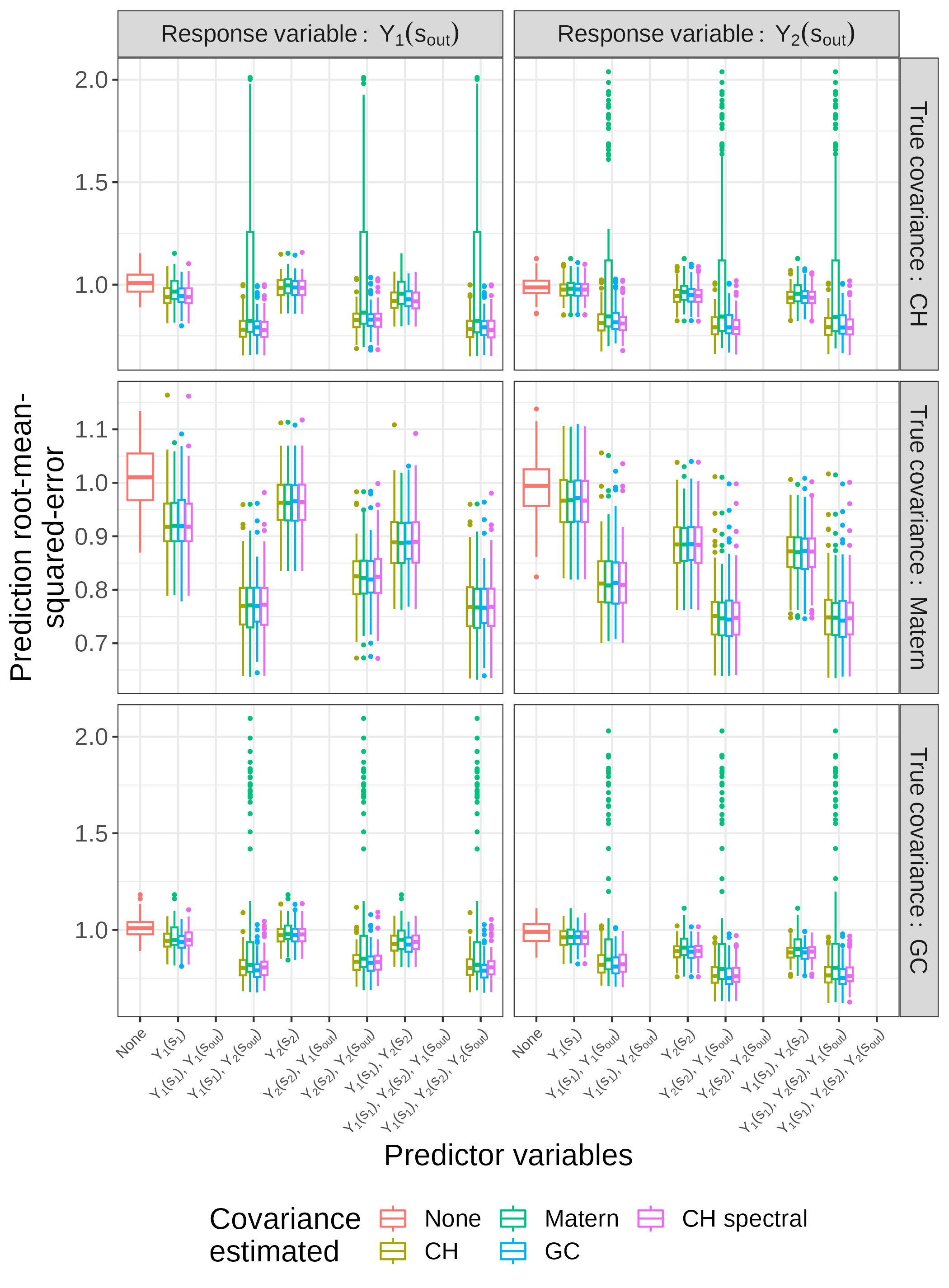
Figure S.1: Simulation prediction error results where the true covariance is CH (Top), Matérn (Middle), and generalized Cauchy (Bottom). This boxplot includes when the variable different from the response variable is used at the prediction sites.

We similarly provide interval summaries in Tables S.1 and S.2. We see that when using the other variable at the predicted locations, the intervals are shorter and do not have as high a coverage. In general, the CH intervals have higher coverage than the Matérn intervals when the true covariance is CH, while the opposite is true when the true covariance is Matérn. In general, coverages when using the other variable at the predicted locations is higher when the true covariance is Matérn compared to when the true covariance is CH. Without observing any colocated data, each model may over-optimistically drive down conditional variances when data for the other variable is available at that site. We next consider the colocated data setting.

Predictor variables	Response variable	95% CI coverage				Average length
		CH	M	GC	SCH	CH	M	GC	SCH
$Y_{1}(\boldsymbol{s}_{1})$	$Y_{1}(\boldsymbol{s}_{out})$	94.2	83.1	95.1	94.0	3.61	2.99	3.73	3.59
$Y_{1}(\boldsymbol{s}_{1})$, $Y_{2}(\boldsymbol{s}_{out})$	$Y_{1}(\boldsymbol{s}_{out})$	88.1	65.1	85.9	89.2	2.69	2.05	2.63	2.72
$Y_{2}(\boldsymbol{s}_{2})$	$Y_{1}(\boldsymbol{s}_{out})$	94.6	83.4	94.2	94.4	3.83	3.12	3.77	3.81
$Y_{2}(\boldsymbol{s}_{2})$, $Y_{2}(\boldsymbol{s}_{out})$	$Y_{1}(\boldsymbol{s}_{out})$	88.7	65.4	85.2	89.8	2.93	2.18	2.71	2.96
$Y_{1}(\boldsymbol{s}_{1})$, $Y_{2}(\boldsymbol{s}_{2})$	$Y_{1}(\boldsymbol{s}_{out})$	93.9	83.0	94.9	93.8	3.51	2.93	3.64	3.49
$Y_{1}(\boldsymbol{s}_{1})$, $Y_{2}(\boldsymbol{s}_{2})$, $Y_{2}(\boldsymbol{s}_{out})$	$Y_{1}(\boldsymbol{s}_{out})$	87.9	65.0	85.9	88.9	2.67	2.04	2.63	2.71
$Y_{1}(\boldsymbol{s}_{1})$	$Y_{2}(\boldsymbol{s}_{out})$	95.0	83.5	95.3	95.0	3.85	3.08	3.90	3.84
$Y_{1}(\boldsymbol{s}_{1})$, $Y_{1}(\boldsymbol{s}_{out})$	$Y_{2}(\boldsymbol{s}_{out})$	88.8	65.5	86.1	90.2	2.88	2.14	3.08	2.93
$Y_{2}(\boldsymbol{s}_{2})$	$Y_{2}(\boldsymbol{s}_{out})$	94.9	83.3	94.6	94.8	3.71	2.99	3.69	3.70
$Y_{2}(\boldsymbol{s}_{2})$, $Y_{1}(\boldsymbol{s}_{out})$	$Y_{1}(\boldsymbol{s}_{out})$	88.7	65.3	85.6	90.0	2.79	2.06	2.62	2.83
$Y_{1}(\boldsymbol{s}_{1})$, $Y_{2}(\boldsymbol{s}_{2})$	$Y_{2}(\boldsymbol{s}_{out})$	94.7	83.3	94.5	94.7	3.66	2.95	3.65	3.65
$Y_{1}(\boldsymbol{s}_{1})$, $Y_{2}(\boldsymbol{s}_{2})$, $Y_{1}(\boldsymbol{s}_{out})$	$Y_{2}(\boldsymbol{s}_{out})$	88.5	65.3	85.6	89.9	2.78	2.06	2.62	2.82

Table S.1: Prediction interval summaries when the true multivariate covariance is CH. We compare estimated CH, Matérn (M), generalized Cauchy (GC), and spectrally-generated CH (SCH) multivariate covariances used for prediction.

Predictor variables	Response variable	95% CI coverage				Average length
		CH	M	GC	SCH	CH	M	GC	SCH
$Y_{1}(\boldsymbol{s}_{1})$	$Y_{1}(\boldsymbol{s}_{out})$	94.4	94.4	95.0	94.3	3.53	3.61	3.53	3.53
$Y_{1}(\boldsymbol{s}_{1})$, $Y_{2}(\boldsymbol{s}_{out})$	$Y_{1}(\boldsymbol{s}_{out})$	90.1	90.8	90.5	90.4	2.70	2.73	2.71	2.71
$Y_{2}(\boldsymbol{s}_{2})$	$Y_{1}(\boldsymbol{s}_{out})$	94.5	94.5	94.3	94.6	3.74	3.74	3.71	3.74
$Y_{2}(\boldsymbol{s}_{2})$, $Y_{2}(\boldsymbol{s}_{out})$	$Y_{1}(\boldsymbol{s}_{out})$	90.5	91.1	89.9	90.8	2.97	3.01	2.88	2.98
$Y_{1}(\boldsymbol{s}_{1})$, $Y_{2}(\boldsymbol{s}_{2})$	$Y_{1}(\boldsymbol{s}_{out})$	94.2	94.1	94.8	94.1	3.37	3.37	3.45	3.37
$Y_{1}(\boldsymbol{s}_{1})$, $Y_{2}(\boldsymbol{s}_{2})$, $Y_{2}(\boldsymbol{s}_{out})$	$Y_{1}(\boldsymbol{s}_{out})$	90.0	90.6	90.5	90.2	2.69	2.72	2.70	2.70
$Y_{1}(\boldsymbol{s}_{1})$	$Y_{2}(\boldsymbol{s}_{out})$	94.9	94.9	95.1	94.9	3.80	3.80	3.85	3.80
$Y_{1}(\boldsymbol{s}_{1})$, $Y_{1}(\boldsymbol{s}_{out})$	$Y_{2}(\boldsymbol{s}_{out})$	90.8	91.3	90.7	91.0	2.95	2.98	2.92	2.95
$Y_{2}(\boldsymbol{s}_{2})$	$Y_{2}(\boldsymbol{s}_{out})$	94.8	94.7	94.7	94.8	3.43	3.43	3.43	3.43
$Y_{2}(\boldsymbol{s}_{2})$, $Y_{1}(\boldsymbol{s}_{out})$	$Y_{1}(\boldsymbol{s}_{out})$	90.8	91.4	90.4	91.0	2.67	2.70	2.61	2.68
$Y_{1}(\boldsymbol{s}_{1})$, $Y_{2}(\boldsymbol{s}_{2})$	$Y_{2}(\boldsymbol{s}_{out})$	94.7	94.6	94.6	94.7	3.36	3.35	3.36	3.36
$Y_{1}(\boldsymbol{s}_{1})$, $Y_{2}(\boldsymbol{s}_{2})$, $Y_{1}(\boldsymbol{s}_{out})$	$Y_{2}(\boldsymbol{s}_{out})$	90.7	91.4	90.5	91.0	2.66	2.69	2.61	2.67

Table S.2: Prediction interval summaries when the true multivariate covariance is Matérn. We compare estimated CH, Matérn (M), generalized Cauchy (GC), and spectrally-generated CH (SCH) multivariate covariances used for prediction.

Predictor variables	Response variable	95% CI coverage				Average length
		CH	M	GC	SCH	CH	M	GC	SCH
$Y_{1}(\boldsymbol{s}_{1})$	$Y_{1}(\boldsymbol{s}_{out})$	94.1	86.4	94.6	91.3	3.63	3.15	3.65	3.42
$Y_{1}(\boldsymbol{s}_{1})$, $Y_{2}(\boldsymbol{s}_{out})$	$Y_{1}(\boldsymbol{s}_{out})$	86.6	68.0	87.8	86.0	2.70	2.12	2.73	2.62
$Y_{2}(\boldsymbol{s}_{2})$	$Y_{1}(\boldsymbol{s}_{out})$	94.6	86.4	94.5	93.0	3.78	3.24	3.77	3.62
$Y_{2}(\boldsymbol{s}_{2})$, $Y_{2}(\boldsymbol{s}_{out})$	$Y_{1}(\boldsymbol{s}_{out})$	87.4	68.2	88.2	88.1	2.89	2.24	2.89	2.86
$Y_{1}(\boldsymbol{s}_{1})$, $Y_{2}(\boldsymbol{s}_{2})$	$Y_{1}(\boldsymbol{s}_{out})$	93.7	86.2	94.5	90.7	3.54	3.08	3.57	3.33
$Y_{1}(\boldsymbol{s}_{1})$, $Y_{2}(\boldsymbol{s}_{2})$, $Y_{2}(\boldsymbol{s}_{out})$	$Y_{1}(\boldsymbol{s}_{out})$	86.4	67.9	87.7	85.8	2.69	2.12	2.72	2.61
$Y_{1}(\boldsymbol{s}_{1})$	$Y_{2}(\boldsymbol{s}_{out})$	95.1	86.9	95.2	94.3	3.79	3.24	3.80	3.68
$Y_{1}(\boldsymbol{s}_{1})$, $Y_{1}(\boldsymbol{s}_{out})$	$Y_{2}(\boldsymbol{s}_{out})$	87.8	68.0	88.6	89.0	2.86	2.20	2.87	2.87
$Y_{2}(\boldsymbol{s}_{2})$	$Y_{2}(\boldsymbol{s}_{out})$	94.9	86.6	95.0	93.5	3.50	3.02	3.49	3.37
$Y_{2}(\boldsymbol{s}_{2})$, $Y_{1}(\boldsymbol{s}_{out})$	$Y_{1}(\boldsymbol{s}_{out})$	87.4	67.9	88.3	88.2	2.63	2.03	2.63	2.62
$Y_{1}(\boldsymbol{s}_{1})$, $Y_{2}(\boldsymbol{s}_{2})$	$Y_{2}(\boldsymbol{s}_{out})$	94.7	86.5	94.8	93.4	3.46	2.99	3.46	3.32
$Y_{1}(\boldsymbol{s}_{1})$, $Y_{2}(\boldsymbol{s}_{2})$, $Y_{1}(\boldsymbol{s}_{out})$	$Y_{2}(\boldsymbol{s}_{out})$	87.4	67.8	88.2	88.1	2.63	2.03	2.62	2.61

Table S.3: Prediction interval summaries when the true multivariate covariance is generalized Cauchy. We compare estimated CH, Matérn (M), generalized Cauchy (GC), and spectrally-generated CH (SCH) multivariate covariances used for prediction.

S.2.2 Colocated design

In this Subsection, we evaluate the setting where $\boldsymbol{s}_{1}=\boldsymbol{s}_{2}$ instead of having the two variables measured at entirely distinct locations. We assume we have $n_{1}=n_{2}=100$ locations. Point prediction results are summarized in Figure S.2. For the most part, the multivariate covariance types perform similarly to each other throughout the three settings. Having both variables available at each of the observed data locations means the covariance $\sigma_{12}$ should be easier to estimate. We summarize the interval performance under the three settings in Tables S.4, S.5, and S.6. Compared to the non-colocated design, interval coverages are better when using the other variable at left out locations.

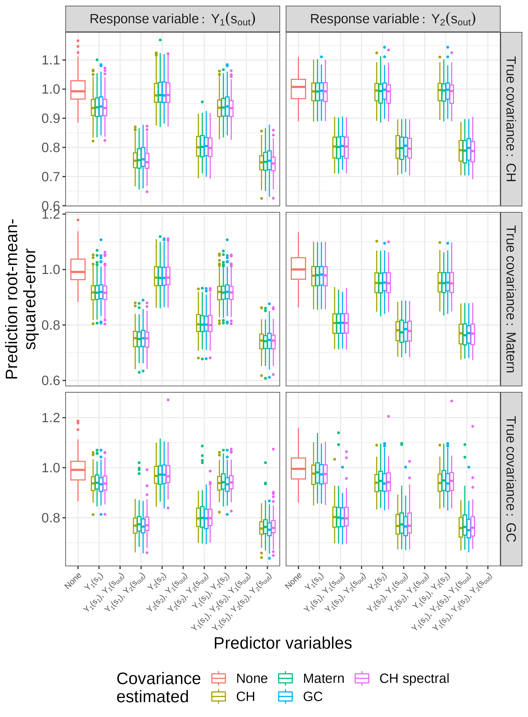
Figure S.2: Simulation prediction error results where the true covariance is CH (Top), Matérn (Middle), and generalized Cauchy (Bottom) and the locations of observed data are colocated.

Predictor variables	Response variable	95% CI coverage				Average length
		CH	M	GC	SCH	CH	M	GC	SCH
$Y_{1}(\boldsymbol{s}_{1})$	$Y_{1}(\boldsymbol{s}_{out})$	94.2	94.1	95.0	94.0	3.60	3.61	3.70	3.58
$Y_{1}(\boldsymbol{s}_{1})$, $Y_{2}(\boldsymbol{s}_{out})$	$Y_{1}(\boldsymbol{s}_{out})$	93.7	93.3	94.6	93.5	2.87	2.85	2.98	2.84
$Y_{2}(\boldsymbol{s}_{2})$	$Y_{1}(\boldsymbol{s}_{out})$	94.8	94.8	94.6	94.6	3.87	3.87	3.83	3.85
$Y_{2}(\boldsymbol{s}_{2})$, $Y_{2}(\boldsymbol{s}_{out})$	$Y_{1}(\boldsymbol{s}_{out})$	94.4	94.0	94.2	94.1	3.10	3.07	3.10	3.08
$Y_{1}(\boldsymbol{s}_{1})$, $Y_{2}(\boldsymbol{s}_{2})$	$Y_{1}(\boldsymbol{s}_{out})$	94.2	94.0	95.0	94.0	3.59	3.60	3.70	3.56
$Y_{1}(\boldsymbol{s}_{1})$, $Y_{2}(\boldsymbol{s}_{2})$, $Y_{2}(\boldsymbol{s}_{out})$	$Y_{1}(\boldsymbol{s}_{out})$	93.6	93.4	94.6	93.5	2.83	2.82	2.94	2.80
$Y_{1}(\boldsymbol{s}_{1})$	$Y_{2}(\boldsymbol{s}_{out})$	94.5	94.2	94.9	94.4	3.87	3.83	3.93	3.85
$Y_{1}(\boldsymbol{s}_{1})$, $Y_{1}(\boldsymbol{s}_{out})$	$Y_{2}(\boldsymbol{s}_{out})$	94.2	93.8	94.8	94.2	3.09	3.05	3.18	3.07
$Y_{2}(\boldsymbol{s}_{2})$	$Y_{2}(\boldsymbol{s}_{out})$	94.1	93.8	93.9	94.0	3.80	3.77	3.80	3.78
$Y_{2}(\boldsymbol{s}_{2})$, $Y_{1}(\boldsymbol{s}_{out})$	$Y_{1}(\boldsymbol{s}_{out})$	93.6	93.1	93.6	93.6	3.02	2.99	3.06	3.00
$Y_{1}(\boldsymbol{s}_{1})$, $Y_{2}(\boldsymbol{s}_{2})$	$Y_{2}(\boldsymbol{s}_{out})$	94.0	93.6	93.9	93.9	3.79	3.75	3.80	3.77
$Y_{1}(\boldsymbol{s}_{1})$, $Y_{2}(\boldsymbol{s}_{2})$, $Y_{1}(\boldsymbol{s}_{out})$	$Y_{2}(\boldsymbol{s}_{out})$	93.6	93.2	93.6	93.6	2.98	2.95	3.02	2.96

Table S.4: Prediction interval summaries when the true multivariate covariance is CH under the colocated design. We compare estimated CH, Matérn (M), generalized Cauchy (GC), and spectrally-generated CH (SCH) multivariate covariances used for prediction.

Predictor variables	Response variable	95% CI coverage				Average length
		CH	M	GC	SCH	CH	M	GC	SCH
$Y_{1}(\boldsymbol{s}_{1})$	$Y_{1}(\boldsymbol{s}_{out})$	94.9	94.2	95.0	94.4	3.52	3.53	3.59	3.52
$Y_{1}(\boldsymbol{s}_{1})$, $Y_{2}(\boldsymbol{s}_{out})$	$Y_{1}(\boldsymbol{s}_{out})$	93.9	93.9	94.8	93.9	2.84	2.85	2.92	2.85
$Y_{2}(\boldsymbol{s}_{2})$	$Y_{1}(\boldsymbol{s}_{out})$	94.8	94.9	94.7	94.8	3.82	3.83	3.81	3.82
$Y_{2}(\boldsymbol{s}_{2})$, $Y_{2}(\boldsymbol{s}_{out})$	$Y_{1}(\boldsymbol{s}_{out})$	94.3	94.4	94.5	94.4	3.12	3.13	3.13	3.12
$Y_{1}(\boldsymbol{s}_{1})$, $Y_{2}(\boldsymbol{s}_{2})$	$Y_{1}(\boldsymbol{s}_{out})$	94.3	94.2	95.0	94.2	3.51	3.52	3.59	3.52
$Y_{1}(\boldsymbol{s}_{1})$, $Y_{2}(\boldsymbol{s}_{2})$, $Y_{2}(\boldsymbol{s}_{out})$	$Y_{1}(\boldsymbol{s}_{out})$	93.8	93.9	94.7	93.8	2.79	2.80	2.87	2.80
$Y_{1}(\boldsymbol{s}_{1})$	$Y_{2}(\boldsymbol{s}_{out})$	94.6	94.5	94.9	94.6	3.82	3.82	3.88	3.82
$Y_{1}(\boldsymbol{s}_{1})$, $Y_{1}(\boldsymbol{s}_{out})$	$Y_{2}(\boldsymbol{s}_{out})$	94.3	94.4	94.8	94.3	3.12	3.12	3.18	3.12
$Y_{2}(\boldsymbol{s}_{2})$	$Y_{2}(\boldsymbol{s}_{out})$	94.2	94.2	94.3	94.2	3.65	3.65	3.66	3.64
$Y_{2}(\boldsymbol{s}_{2})$, $Y_{1}(\boldsymbol{s}_{out})$	$Y_{1}(\boldsymbol{s}_{out})$	93.6	93.8	93.9	93.7	2.95	2.95	2.97	2.94
$Y_{1}(\boldsymbol{s}_{1})$, $Y_{2}(\boldsymbol{s}_{2})$	$Y_{2}(\boldsymbol{s}_{out})$	94.1	94.1	94.3	94.2	3.64	3.64	3.66	3.63
$Y_{1}(\boldsymbol{s}_{1})$, $Y_{2}(\boldsymbol{s}_{2})$, $Y_{1}(\boldsymbol{s}_{out})$	$Y_{2}(\boldsymbol{s}_{out})$	93.6	93.7	94.0	93.7	2.89	2.90	2.92	2.89

Table S.5: Prediction interval summaries when the true multivariate covariance is Matérn under the colocated design. We compare estimated CH, Matérn (M), generalized Cauchy (GC), and spectrally-generated CH (SCH) multivariate covariances used for prediction.

Predictor variables	Response variable	95% CI coverage				Average length
		CH	M	GC	SCH	CH	M	GC	SCH
$Y_{1}(\boldsymbol{s}_{1})$	$Y_{1}(\boldsymbol{s}_{out})$	94.5	94.0	94.6	93.2	3.63	3.61	3.65	3.50
$Y_{1}(\boldsymbol{s}_{1})$, $Y_{2}(\boldsymbol{s}_{out})$	$Y_{1}(\boldsymbol{s}_{out})$	93.7	91.0	94.3	90.6	2.92	2.80	2.96	2.72
$Y_{2}(\boldsymbol{s}_{2})$	$Y_{1}(\boldsymbol{s}_{out})$	94.9	94.5	94.9	93.7	3.82	3.77	3.83	3.69
$Y_{2}(\boldsymbol{s}_{2})$, $Y_{2}(\boldsymbol{s}_{out})$	$Y_{1}(\boldsymbol{s}_{out})$	94.4	91.6	94.8	91.8	3.10	2.96	3.14	2.89
$Y_{1}(\boldsymbol{s}_{1})$, $Y_{2}(\boldsymbol{s}_{2})$	$Y_{1}(\boldsymbol{s}_{out})$	94.3	93.9	94.6	92.9	3.62	3.60	3.65	3.49
$Y_{1}(\boldsymbol{s}_{1})$, $Y_{2}(\boldsymbol{s}_{2})$, $Y_{2}(\boldsymbol{s}_{out})$	$Y_{1}(\boldsymbol{s}_{out})$	93.7	91.0	94.2	90.4	2.88	2.76	2.91	2.66
$Y_{1}(\boldsymbol{s}_{1})$	$Y_{2}(\boldsymbol{s}_{out})$	94.7	93.9	94.7	93.7	3.85	3.75	3.83	3.71
$Y_{1}(\boldsymbol{s}_{1})$, $Y_{1}(\boldsymbol{s}_{out})$	$Y_{2}(\boldsymbol{s}_{out})$	94.5	91.3	94.8	91.6	3.13	2.94	3.13	2.90
$Y_{2}(\boldsymbol{s}_{2})$	$Y_{2}(\boldsymbol{s}_{out})$	93.9	93.3	94.3	92.7	3.63	3.57	3.64	3.51
$Y_{2}(\boldsymbol{s}_{2})$, $Y_{1}(\boldsymbol{s}_{out})$	$Y_{1}(\boldsymbol{s}_{out})$	93.6	90.4	94.1	90.7	2.92	2.78	2.95	2.72
$Y_{1}(\boldsymbol{s}_{1})$, $Y_{2}(\boldsymbol{s}_{2})$	$Y_{2}(\boldsymbol{s}_{out})$	93.9	93.2	94.3	92.6	3.62	3.57	3.64	3.50
$Y_{1}(\boldsymbol{s}_{1})$, $Y_{2}(\boldsymbol{s}_{2})$, $Y_{1}(\boldsymbol{s}_{out})$	$Y_{2}(\boldsymbol{s}_{out})$	93.6	90.4	94.1	90.2	2.88	2.74	2.91	2.67

Table S.6: Prediction interval summaries when the true multivariate covariance is generalized Cauchy under the colocated design. We compare estimated CH, Matérn (M), generalized Cauchy (GC), and spectrally-generated CH (SCH) multivariate covariances used for prediction.

S.3 Additional Data Analysis Plots

In Figure S.3, we plot the estimated correlation and cross-correlation functions. While the Matérn and CH functions behave similarly near the origin, they behave quite differently in their tails.

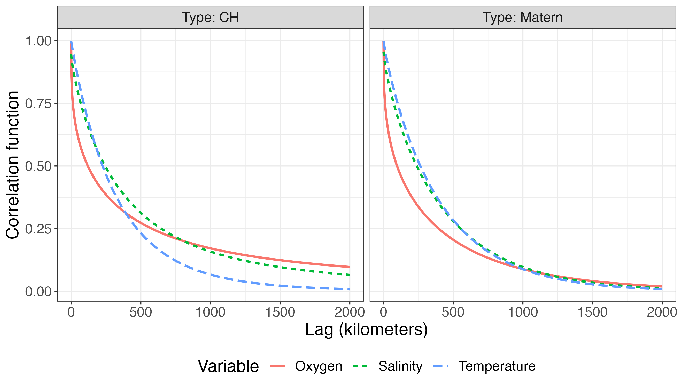
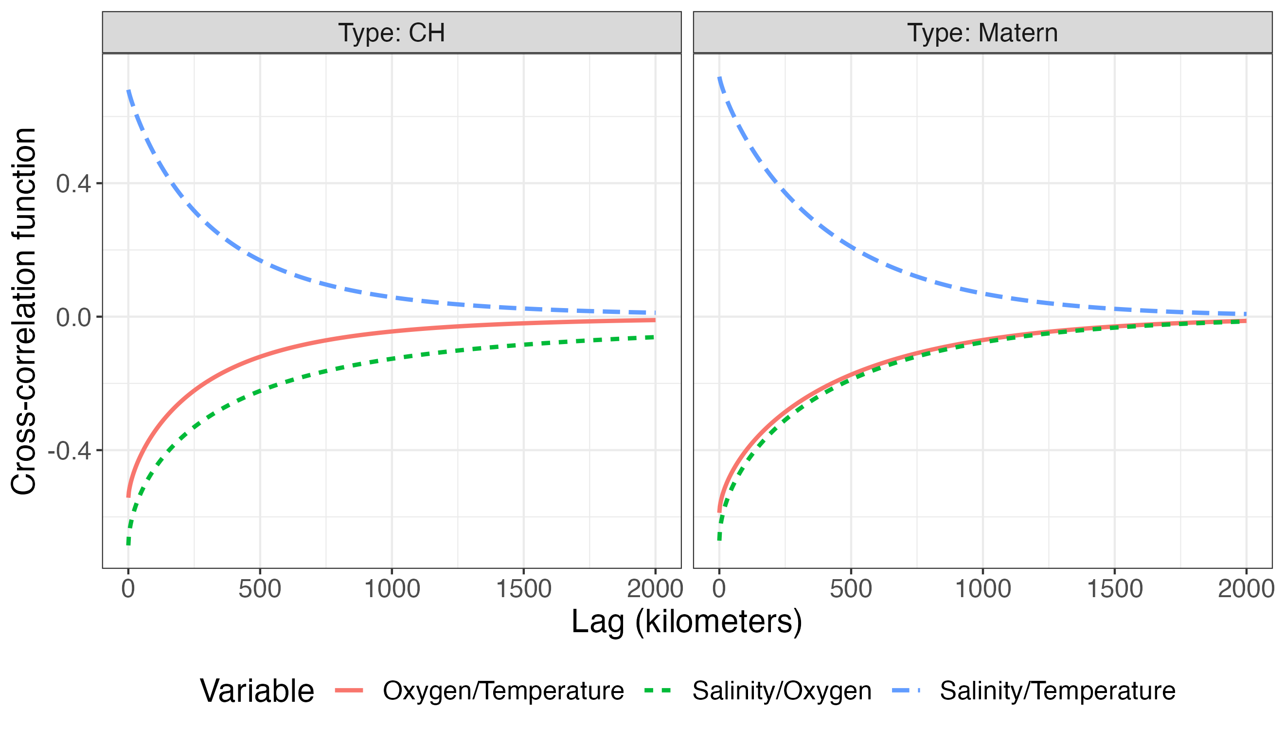
Figure S.3: Estimated correlation (Left) and cross-correlation (Right) functions for the Argo data based on the CH and Matérn cross-covariances. Note that the colors and type of line represent different things in the two panels.

References

- Alegría et al., (2021) Alegría, A., Emery, X., and Porcu, E. (2021). Bivariate Matérn covariances with cross-dimple for modeling coregionalized variables. Spatial Statistics, 41:100491.
- Alegría et al., (2019) Alegría, A., Porcu, E., Furrer, R., and Mateu, J. (2019). Covariance functions for multivariate Gaussian fields evolving temporally over planet earth. Stochastic Environmental Research and Risk Assessment, 33:1593–1608.
- Apanasovich et al., (2012) Apanasovich, T. V., Genton, M. G., and Sun, Y. (2012). A valid Matérn class of cross-covariance functions for multivariate random fields with any number of components. Journal of the American Statistical Association, 107(497):180–193.
- Argo, (2023) Argo (2023). Argo float data and metadata from Global Data Assembly Centre (Argo GDAC). 10.17882/42182.
- Bachoc et al., (2022) Bachoc, F., Porcu, E., Bevilacqua, M., Furrer, R., and Faouzi, T. (2022). Asymptotically equivalent prediction in multivariate geostatistics. Bernoulli, 28(4).
- Baricz and Ismail, (2013) Baricz, Á. and Ismail, M. E. (2013). Turán type inequalities for Tricomi confluent hypergeometric functions. Constructive Approximation, 37:195–221.
- Bateman, (1954) Bateman, H. (1954). Tables of Integral Transforms, volume 1. McGraw-Hill book company.
- Berg et al., (1984) Berg, C., Christensen, J. P. R., and Ressel, P. (1984). Harmonic analysis on semigroups: theory of positive definite and related functions, volume 100. Springer.
- Bevilacqua et al., (2015) Bevilacqua, M., Hering, A. S., and Porcu, E. (2015). On the flexibility of multivariate covariance models: Comment on the paper by Genton and Kleiber. Statistical Science, 30(2):167–169.
- Bhukya et al., (2018) Bhukya, R., Akavaram, V., and Qi, F. (2018). Some inequalities of the Turán type for confluent hypergeometric functions of the second kind. HAL, 2018.
- Chen et al., (2021) Chen, W., Genton, M. G., and Sun, Y. (2021). Space-time covariance structures and models. Annual Review of Statistics and Its Application, 8:191–215.
- Dey et al., (2022) Dey, D., Datta, A., and Banerjee, S. (2022). Graphical Gaussian process models for highly multivariate spatial data. Biometrika, 109(4):993–1014.
- DLMF, (2021) DLMF (2021). NIST Digital Library of Mathematical Functions. http://dlmf.nist.gov/, Release 1.1.3 of 2021-09-15. F. W. J. Olver, A. B. Olde Daalhuis, D. W. Lozier, B. I. Schneider, R. F. Boisvert, C. W. Clark, B. R. Miller, B. V. Saunders, H. S. Cohl, and M. A. McClain, eds.
- Eddelbuettel and Francois, (2023) Eddelbuettel, D. and Francois, R. (2023). RcppGSL: ‘Rcpp’ integration for ‘GNU GSL’ vectors and matrices. R package version 0.3.13.
- Emery et al., (2016) Emery, X., Arroyo, D., and Porcu, E. (2016). An improved spectral turning-bands algorithm for simulating stationary vector Gaussian random fields. Stochastic environmental research and risk assessment, 30:1863–1873.
- Emery and Porcu, (2023) Emery, X. and Porcu, E. (2023). The Schoenberg kernel and more flexible multivariate covariance models in Euclidean spaces. Computational and Applied Mathematics, 42(4):148.
- Emery et al., (2022) Emery, X., Porcu, E., and White, P. (2022). New validity conditions for the multivariate Matérn coregionalization model, with an application to exploration geochemistry. Mathematical Geosciences, 54(6):1043–1068.
- Galassi, (2009) Galassi, M., editor (2009). GNU scientific library reference manual: for GSL version 1.12. Network Theory, Bristol, 3. ed edition.
- Giglio et al., (2018) Giglio, D., Lyubchich, V., and Mazloff, M. R. (2018). Estimating oxygen in the Southern Ocean using Argo temperature and salinity. Journal of Geophysical Research: Oceans, 123(6):4280–4297.
- Gneiting et al., (2010) Gneiting, T., Kleiber, W., and Schlather, M. (2010). Matérn cross-covariance functions for multivariate random fields. Journal of the American Statistical Association, 105(491):1167–1177.
- Johnson et al., (2020) Johnson, K. S., Riser, S. C., Boss, E. S., Talley, L. D., Sarmiento, J. L., Swift, D. D., Plant, J. N., Maurer, T. L., Key, R. M., Williams, N. L., Wanninkhof, R. H., Dickson, A. G., Feely, R. A., and Russell, J. L. (2020). SOCCOM float data - Snapshot 2023-08-28.
- King, (2009) King, F. W. (2009). Hilbert Transforms. Cambridge University Press.
- Kleiber, (2017) Kleiber, W. (2017). Coherence for multivariate random fields. Statistica Sinica, pages 1675–1697.
- Kleiber and Nychka, (2012) Kleiber, W. and Nychka, D. (2012). Nonstationary modeling for multivariate spatial processes. Journal of Multivariate Analysis, 112:76–91.
- Korte-Stapff et al., (2022) Korte-Stapff, M., Yarger, D., Stoev, S., and Hsing, T. (2022). A multivariate functional-data mixture model for spatio-temporal data: inference and cokriging. arXiv:2211.04012.
- Krock et al., (2023) Krock, M. L., Kleiber, W., Hammerling, D., and Becker, S. (2023). Modeling massive highly multivariate nonstationary spatial data with the basis graphical lasso. Journal of Computational and Graphical Statistics, 0(0):1–16.
- Kuusela and Stein, (2018) Kuusela, M. and Stein, M. L. (2018). Locally stationary spatio-temporal interpolation of Argo profiling float data. Proceedings of the Royal Society A: Mathematical, Physical and Engineering Sciences, 474(2220).
- Li and Zhang, (2011) Li, B. and Zhang, H. (2011). An approach to modeling asymmetric multivariate spatial covariance structures. Journal of Multivariate Analysis, 102(10):1445–1453.
- Ma and Bhadra, (2022) Ma, P. and Bhadra, A. (2022). Beyond Matérn: On a class of interpretable Confluent Hypergeometric covariance functions. Journal of the American Statistical Association, pages 1–14.
- Matsumoto et al., (2022) Matsumoto, G. I., Johnson, K. S., Riser, S., Talley, L., Wijffels, S., and Hotinski, R. (2022). The Global Ocean Biogeochemistry (GO-BGC) array of profiling floats to observe changing ocean chemistry and biology. Marine Technology Society Journal, 56(3):122–123.
- Moreva and Schlather, (2023) Moreva, O. and Schlather, M. (2023). Bivariate covariance functions of Pólya type. Journal of Multivariate Analysis, 194:105099.
- Porcu et al., (2018) Porcu, E., Bevilacqua, M., and Hering, A. S. (2018). The Shkarofsky-Gneiting class of covariance models for bivariate Gaussian random fields. Stat, 7(1):e207.
- Porcu et al., (2023) Porcu, E., Bevilacqua, M., Schaback, R., and Oates, C. J. (2023). The Matérn model: A journey through statistics, numerical analysis and machine learning. arXiv:2303.02759.
- Porcu et al., (2021) Porcu, E., Furrer, R., and Nychka, D. (2021). 30 years of space–time covariance functions. Wiley Interdisciplinary Reviews: Computational Statistics, 13(2):e1512.
- Stein, (1999) Stein, M. L. (1999). Interpolation of Spatial Data: Some Theory for Kriging. Springer Science & Business Media.
- Wong et al., (2020) Wong, A. P., Wijffels, S. E., Riser, S. C., Pouliquen, S., Hosoda, S., Roemmich, D., Gilson, J., Johnson, G. C., Martini, K., Murphy, D. J., et al. (2020). Argo data 1999–2019: Two million temperature-salinity profiles and subsurface velocity observations from a global array of profiling floats. Frontiers in Marine Science, 7:700.
- Yarger et al., (2023) Yarger, D., Stoev, S., and Hsing, T. (2023). Multivariate Matérn models – A spectral approach. arXiv:2309.02584.
- Zhang, (2004) Zhang, H. (2004). Inconsistent estimation and asymptotically equal interpolations in model-based geostatistics. Journal of the American Statistical Association, 99(465):250–261.