Position control of an acoustic cavitation bubble by reinforcement learning

Abstract

A control technique is developed via Reinforcement Learning that allows arbitrary controlling of the position of an acoustic cavitation bubble in a dual-frequency standing acoustic wave field. The agent must choose the optimal pressure amplitude values to manipulate the bubble position in the range of $x/\lambda_{0}\in[0.05,0.25]$. To train the agent an actor-critic off-policy algorithm (Deep Deterministic Policy Gradient) was used that supports continuous action space, which allows setting the pressure amplitude values continuously within $0$ and $1\,\mathrm{bar}$. A shaped reward function is formulated that minimizes the distance between the bubble and the target position and implicitly encourages the agent to perform the position control within the shortest amount of time. In some cases, the optimal control can be 7 times faster than the solution expected from the linear theory.

1 Introduction

The irradiation of the liquid domain with high-frequency and high-intensity ultrasound results in the forming of thousands of micron-sized radially pulsating bubbles. The collapse of these bubbles induces chemical reactions, which is the keen interest of sonochemistry [1]. Despite the great potential of various applications [2, 3, 4, 5, 6, 7], the biggest challenge, the scale-up of applications feasible for industrial sizes, is still unsolved [8]. The attenuation of the sound waves in the densely packed bubble clusters is one of the main limitations [9, 10] and the spurious interaction of the bubbles with the container. Controlling the dynamics of bubble clusters via acoustic manipulation methods; for example, the positioning of bubbles within the clusters, can be a possible solution to overcome such limitations.

Although acoustic manipulation methods are extensively used for solid particles in various applications, such as particle manipulation [11, 12, 13, 14], pattern formation [15] and micro-assembly [16], the utilization of such control techniques is not widespread in the literature in the case of bubble clusters. Only elementary techniques have been applied to cluster control, such as on/off control [17, 18] or bi-frequency driving to avoid spatial instability [19, 20].

The traditional acoustic manipulation devices create a simple pattern of standing waves in a chamber or channel [11]. In such patterns, fixed trapping points (or lines) exist, e.g., pressure nodes and antinodes, where the mean acoustic radiation force is zero. The external forces drive the particles to these fixed positions. Either by controlling the phase or intensity of the transducers or by switching between resonance modes, the wave field is transformed, and the trapping points can be modified; thus, the position of the particles can be controlled [12, 13]. A possible method of particle manipulation is the application of phase-controllable ultrasonic standing waves. In this case, a pair of ultrasonic transducers is applied, and the relative phase between the generated sinusoidal signal is varied to change the position of nodes and antinodes. Abe et al. [21] achieved the control of bubble motion by using this technique for a single bubble in an acoustic standing wave.

Simple control methods are possible for bubbles; however, these techniques are limited to weak pressure amplitude, when the bubbles are trapped by either the node or the antinode. The application of high-intensity, multi-frequency driving allows a more general solution; however, the translational motion becomes much more complex; e.g., the bubble may exhibit periodic and chaotic translational oscillations [22, 23, 24, 25], or the bubble can break up [26]. Therefore, position control may require more complex manipulation of the acoustic field [18, 27, 20, 17], which might be well beyond simple intuitions.

The aim is to seek robust control that allows arbitrarily positioning a bubble in a standing wave field, by using reinforcement learning (RL). Reinforcement learning can be seen as a method to control nonlinear systems, which does not rely on analytical knowledge of the underlying dynamical systems. A large number of RL algorithms have been developed in the last decade. These advanced RL algorithms use (deep) neural networks as function approximators that allow them to operate over discrete and continuous state and action spaces; therefore, complex control tasks can be solved [28, 29, 30, 31, 32]. In the present paper, this kind of manipulation is achieved by applying dual-frequency excitation [33, 34, 35, 36, 37] and tuning the pressure amplitude values in discrete timesteps.

2 Mathematical Model

The coupled radial and translational motion of an acoustic cavitation bubble is described by two coupled ordinary differential equations [38]. The first one is the Keller–Miksis equation [39], which is a second-order nonlinear differential equation that describes the radial oscillation of a spherical bubble. The equation is written as

$$\left(1-\frac{\dot{R}}{c_{L}}\right)R\ddot{R}+\left(1-\frac{\dot{R}}{3c_{L}}\right)\frac{3}{2}\dot{R}^{2}\ =\\ \left(1+\frac{\dot{R}}{c_{L}}+\frac{R}{c_{L}}\frac{d}{dt}\right)\frac{\left(p_{L}-p(x,t)\right)}{\rho_{L}}+\frac{\dot{x}^{2}}{4},$$ (1)

where $R$ and $x$ are the instantaneous bubble radius and its position, respectively. Furthermore, $\rho_{L}=998\,\mathrm{kg/m^{3}}$ is the liquid density, $c_{L}=1500\,\mathrm{m/s}$ is the speed of sound and $p(x,t)$ is the pressure at the centre of the bubble. The dots stand for the derivative with respect to the time. The liquid pressure at the bubble wall is given as

$$p_{L}=p_{G}-\frac{2\sigma}{R}-4\mu_{L}\frac{\dot{R}}{R},$$ (2)

where $\sigma=0.0725\,\mathrm{N/m}$ and $\mu_{L}=0.001\,\mathrm{Pa\,s}$ are the surface tension and the liquid dynamic viscosity, respectively. The gas pressure $p_{G}$ is assumed to obey a polytropic state of change

$$p_{G}=\left(\frac{2\sigma}{R_{0}}+P_{\infty}\right)\left(\frac{R_{0}}{R}\right)^{3n},$$ (3)

where $n=1.4$ is the polytropic exponent and $R_{0}=60\,\mathrm{\mu m}$ is the equilibrium bubble radius.

The translational motion of the bubble is described as [38, 40, 25]

$$R\ddot{x}+3\dot{R}\dot{x}=\frac{3F_{ex}(x,t)}{2\pi\rho_{L}R^{2}},$$ (4)

where $F_{ex}(x,t)$ is the sum of the instantaneous external forces acting on the bubble; namely, the primary Bjerknes force [41]

$$F_{B1}=-V(t)\nabla p(x,t),$$ (5)

and the drag force [42]

$$F_{D}=-12\pi\mu_{L}R\left(\dot{x}-v_{ex}(x,t)\right).$$ (6)

In the above equations, $V(t)$ is the volume of the bubble, $\nabla p(x,t)$ is the pressure gradient and $v_{ex}(x,t)$ is the velocity induced by the acoustic radiation. From Eqs. (4)-(6), one can observe that the manipulation of the acoustic field properties allows the position control of the bubble.

The acoustic field is assumed to be the sum of two standing waves

$$\begin{split}p(x,t)=P_{0}&+P_{A0}\sin(k_{0}x)\sin(\omega_{0}t)\\ &+P_{A1}\sin(k_{1}x)\sin(\omega_{1}t),\end{split}$$ (7)

where $P_{0}=1\,\mathrm{bar}$ is the ambient pressure, $P_{A0}$ and $P_{A1}$ are the pressure amplitudes, $\omega_{0}=2\pi f_{0}$ and $\omega_{1}=2\pi f_{1}$ are the angular frequencies, $k_{0}=2\pi/\lambda_{0}$ and $k_{1}=2\pi/\lambda_{1}$ are the wavenumbers. Note that $\lambda_{0}$ and $\lambda_{1}$ are the wavelengths correspond to the excitation frequencies $f_{0}=25\,\mathrm{kHz}$ and $f_{1}=50\,\mathrm{kHz}$, respectively.

The mathematical model is solved numerically by introducing dimensionless variables; namely, the dimensionless bubble radius $y_{1}=R/R_{0}$, the dimensionless position $\xi=x/\lambda_{0}$ and their derivatives with respect to the dimensionless time $\tau=t/(2\pi/\omega_{0})$. The dimensionless system of equations is given in our previous paper; see [43]. The model is implemented in Python and at each environment step it was solved by the initial value problem solver LSODA included SciPy computational library. The absolute and relative tolerance was set to $10^{-10}$. To enhance computational speed, the numba JIT compiler [44] was used to translate the ODE functions implemented in Python to optimized machine code at runtime.

2.1 Overview of the dynamical features

According to the linear theory, in a weak acoustic field, bubbles are attracted to either the pressure nodes or antinodes depending on their resonance size and excitation frequency [41]. In the present study, the bubble size ($R_{0}=60\,\mathrm{\mu m}$) is chosen to be below the resonant sizes corresponding to the excitation frequencies ($R_{0,Res}=131\,\mathrm{\mu m}$ at $f_{0}=25\,\mathrm{kHz}$ and $R_{1,Res}=66\,\mathrm{\mu m}$ at $f_{1}=50\,\mathrm{kHz}$); thus, the bubble is attracted by the pressure antinodes, indicated by the arrows in Fig. 1. The pressure amplitude corresponding to the lower and higher frequencies are coloured by red and blue, respectively. The filled circles denote the antinodes. An antinode corresponding to the higher frequency component is located at $x/\lambda_{0}=0.125$. Below this threshold, between black and blue dashed lines, by increasing either $P_{A0}$ or $P_{A1}$, the expected translational direction is positive (blue and red arrow). The antinode corresponding to the lower frequency is located at $x/\lambda_{0}=0.25$. Between the blue and red dashed lines, the translational direction is either positive or negative depending on the magnitudes of the pressure amplitudes.

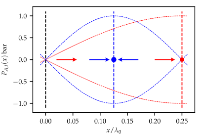
Figure 1: Schematic illustration of the acoustic field and the expected direction of the translational motion by linear theory.

To get an insight into the non-linear translational dynamics, one-dimensional bifurcation diagrams were calculated at fixed $P_{A1}$ values by changing $P_{A0}$ between $0.1\,\mathrm{bar}$ and $0.6\,\mathrm{bar}$ with a resolution of 151 steps. At every parameter combination, 5 initial positions were prescribed in the range of $x/\lambda_{0}\in(0.05,0.2)$, and then initial value problem computations were carried out. The first 8192 acoustic cycles were treated as transients and these results were discarded. Only the (converged) trajectory segments obtained during the last 256 acoustic cycles were evaluated.

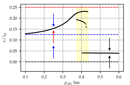
Figure 2: Mean bubble positions as a function of the pressure amplitude $P_{A0}$ at constant $P_{A1}=0.1\,\mathrm{bar}$. The horizontal dashed lines correspond to the pressure antinodes and nodes. The arrows indicate the direction of the translational motion.

An example is given in Fig. 2, where the mean dimensionless displacement of the bubble is plotted as a function of the pressure amplitude $P_{A0}$. The horizontal dashed lines correspond to the pressure antinodes and nodes, see again Fig. 1. At low-pressure amplitude, the bubble translates to an intermediate equilibrium position between the antinodes. This is in agreement with the linear theory; thus, the expected directions can be figured out according to Fig. 1. The increasing pressure amplitude results in co-existing solutions (highlighted by the yellow rectangle). In addition, above pressure amplitude $P_{A0}=0.43\,\mathrm{bar}$, only one stable solution exists around $x/\lambda_{0}=0.4$. Thus, the combination of the dual frequency in the highly nonlinear regime may induce Bjerknes force that points in the opposite direction (black arrows) compared to the linear theory. The further increase of the pressure amplitude causes oscillatory solutions [43]. The above observation implies that the bubble position can be controlled arbitrarily between approximately $x/\lambda_{0}=0.05$ and $x/\lambda_{0}=0.25$ by the proper tuning of the pressure amplitude components. This simple example demonstrates that exploiting non-linear dynamics allows more flexibility in position control. However, in the general case, where both $P_{A0}$ and $P_{A1}$ are tuned, the process is highly non-trivial. Thus, the aim is to develop a control system capable of arbitrarily positioning the bubble from any randomized initial position to any randomized final position. The idea is to use a deep neural network trained via reinforcement learning, to develop such a controller.

3 The reinforcement learning framework

To apply reinforcement learning, the above-described position control problem is formulated as a Markov decision process (MDP). The main elements of an MDP are the state, the action and the reward function [28, 29]. $S$ and $A$ represent the state space and the action space, respectively and $R:S\times A\times S\rightarrow\mathbb{R}$ is the reward function. At each step, the agent observes the state $s\in S$ of the environment and chooses an action $a\in A$. One step is 50 acoustic cycles. Then, the environment moves to a new state $s^{\prime}\in S$, and the agent receives the reward signal $r=R(s,a,s^{\prime})$ from the environment. The reward function depends on the actual state of the environment, the action taken at that state, and the next state of the environment. The function that maps states to actions is the policy $a=\pi(s)$. The goal of the agent is to find a policy that maximizes the expected discounted return $R=\sum_{k=0}^{\infty}\gamma^{k}r_{k}$. The discount factor $\gamma\in(0,1)$ ensures the convergence of the infinite sum of reward. In the present paper, the agent controls the pressure amplitudes, and the environment is the bubble itself in the acoustic field. The elements of the MDP for the present problem are discussed below.

State $S$ represents the observable quantities for the agent at each timestep. In the present paper, the state is assumed to be partially observable; thus, only bubble position values are observed. The first quantity is the desired (target) $x_{T}$ position in a given trial (episode). The next observed quantity is the actual position of the bubble $x_{t}$. To help the agent infer the direction and the velocity of the movement, the previous position value $x_{t-1}$ is also encoded in the actual observation. In the present paper, the maximum displacement of the bubble is $\lambda_{0}/4$; thus, the position values are normalized by the maximum of the observation limit to rescale the numerical values in the range of $[0,1]$. Hereby, the state vector is defined as

$$s=\left[\dfrac{4x_{T}}{\lambda_{0}},\dfrac{4x_{t}}{\lambda_{0}},\dfrac{4x_{t-1}}{\lambda_{0}}\right].$$ (8)

Action Space $A$ represents a set of actions that are available for the agent. According to the present control problem, the pressure amplitude values are changed in discrete timesteps; thus, the action space dimension is 2, where each value represents one of the two components of the pressure field

$$a=[P_{A0},P_{A1}].$$ (9)

The pressure amplitude values are in the range of $P_{A0},P_{A1}\in[P_{A,min},P_{A,max}]$. Note that the pressure amplitude values are a piecewise constant function of time. One step of the environment represents 50 excitation periods ($50\tau$). Within each of these intervals, the pressure amplitude values are fixed. This time domain is higher than the transient regime required to establish a standing wave pattern in typical reactor scales; thus, the omission of complete acoustic simulation is a reasonable simplification.

The immediate reward $r$ is the only feedback from the environment for the agent that represents how bad or good the last action was. To minimize the position error, the reward signal is defined as a shaped reward function as

$$r_{1}=1-\left(\dfrac{d}{d_{max}}\right)^{k},$$ (10)

where $d=|x_{T}-x_{t}|$ is the distance between the actual and the target position, $d_{max}$ is the maximum (possible) distance defined as

$$d_{max}=\max\left(x_{max}-x_{T},x_{T}-x_{min}\right),$$ (11)

and $k=0.2$ is the exponent, and the observation limits are $x_{min}=0.05\lambda_{0}$ and $x_{max}=0.25\lambda_{0}$.

Parameter	Notation	Value
Equilibrium bubble radius	$R_{0}$	$60\,\mathrm{\mu m}$
Low frequency component	$f_{0}$	$25\,\mathrm{kHz}$
High frequency component	$f_{1}$	$50\,\mathrm{kHz}$
Observation space dimension		$(3,1)$
Observation space limits	$[x_{min},x_{max}]$	$[0.05,0.25]\cdot\lambda_{0}$
Action space dimension		$(2,1)$
Action space limits	$[P_{A,min},P_{A,max}]$	$[0,1\,\mathrm{bar}]$
Action duration	$\Delta\tau$	$50\tau$
Episode length	$N_{t}$	12$\Delta\tau$

Table 1: Properties of the environment.

The environment is implemented as an OpenAI GYM-like environment [45], which is built on top of the model implementation presented in Section II. The chosen algorithm used to train the agent is the deep deterministic policy gradient (DDPG) [46, 32]. It is an off-policy, actor-critic algorithm that uses deep function approximations. DDPG can learn policies in continuous state and action spaces. The algorithm is implemented in Python by using the Pytorch deep-learning framework [47]. The implementation is verified by comparing the performance with the implementation of Clean RL [48] on benchmark problems provided by the Gym API. Although, the above formalism allows customizable properties (frequency components, bubble size, time-step length, etc.) of the environment; the present paper demonstrates position control for one specific set of parameters, which are summarized in Table 1.

3.1 Training of the agent

At the beginning of the episodes, the bubble was assumed to be at rest, and the initial position was randomly prescribed ($R=R_{0}$, $\dot{R}=0$). Each episode terminates if the agent reaches the maximum allowed steps per episode or the target position is reached with a tolerance of $E_{x/\lambda_{0}}=0.01$. At every step, the experience ($e_{t}=(s_{t},a_{t},r_{t},s_{t+1})$) is collected in the replay buffer. Batches of experiences are chosen randomly from the replay buffer to optimize the policy network according to the DDPG algorithm [32]. To ensure the exploration, a Gaussian noise is applied. The applied hyperparameters are summarized in Table 2. Keeping the hyperparameters fixed, the size of the neural network is optimized.

The policy network (actor) has as many input neurons as the size of the state vector. The output layer has two nodes for the two amplitude values with an activation function of tangent hyperbolic to scale the output values ($\hat{y}_{i}$) in the range of [-1,1]. Then, it is rescaled to actions (pressure amplitude) as

$$a_{i}=P_{Ai}=\dfrac{P_{A,max}-P_{A,min}}{2}\cdot\hat{y}_{i}+\dfrac{P_{A,max}+P_{A,min}}{2}.$$ (12)

The critic network has $N+2$ input neurons (state and actions) and 1 output neuron for the action value.

The optimal number of hidden layers and the number of neurons per layer are optimized by gradually increasing the network complexity and evaluating the training performance. Figure 3 shows the smoothed (exponential moving averaged) of the episodic return as a function of training steps for different network architectures and activation functions. Note that the theoretical maximum for an infinite time horizon is $R_{max}\approx\lim_{r\rightarrow\infty}{\sum_{k=0}^{\infty}\gamma^{k}r_{k}}=100$. The top panel shows the episodic reward as a function of steps for different network structures with a rectified linear unit (ReLU) as activation in the hidden layers. The highest reward and the fastest convergence are achieved using two hidden layers with 128 neurons per hidden layer. The increasing model complexity resulted in poor performance. It is worth mentioning that with one hidden layer, the algorithm is not converged (not shown here) for the present problem. Using tangent hyperbolic (Tanh) as activation in the hidden layers, slightly better convergence is achieved (see the bottom diagram).

Hyperparameter	Value
Learning rate	$2.5\cdot 10^{-4}$
Discount factor	$0.99$
Batch size	$256$
Buffer size	$10\,000$
Soft update weight ($\tau$)	$5\cdot 10^{-3}$
Exploration noise	0.1

Table 2: Hyperparameters of the agent.

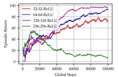
(a)

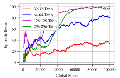
(b)

Figure 3: The episodic return as a function of the (global) timesteps for ReLU and Tanh activation in the hidden layers.

The maximization of an improperly specified reward may lead to false policy from the point of view of the main objective, which is to achieve position control within the shortest time. Therefore, the episode length (exponential moving averaged) for the top three models is plotted in Figure 4. The results show that shorter episodes, i.e., fastest position control can be achieved using Tanh activation in the hidden layers.

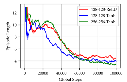
Figure 4: The episode length as a function of the (global) timesteps for the three best models.

4 Case studies

For further investigations, the trained model with the highest complexity (256-256-Tanh) is chosen. To evaluate the model performance, numerous simulations were carried out with various initial and target positions. The pressure amplitudes were chosen according to the trained policy. The results are visualized in Figure 5, where the total number of steps required for position control is plotted as a function of the initial $x_{0}/\lambda_{0}$ and target $x_{T}/\lambda_{0}$ bubble positions. The applied resolution is $x_{0}\times x_{T}=101\times 101$. The figure shows that the position control was successful in the majority of the parameter space (97%), and the bubble was driven to the target position in less than 15 steps, i.e.; less than $15\times 50=750$ acoustic cycles.

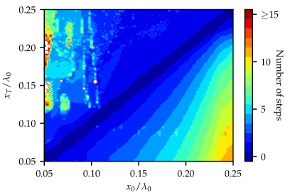
Figure 5: The number of steps required to drive the bubble from initial position $x_{0}/\lambda_{0}$ to target position $x_{T}/\lambda_{0}$.

Figure 6 shows a specific test case when the bubble is driven from one side of the space domain to the other. On the top panel, the trajectory of the bubble (black curve) is plotted as a function of the acoustic cycles, while the bottom panel shows the applied pressure amplitude values. The green horizontal dashed lines denote the thresholds for successful control around the target position $x_{T}/\lambda_{0}=0.25$. The trajectory shows 3 different kinds of segments. At $x/\lambda_{0}=0.05$ the agent chooses high $P_{A0}$ and zero $P_{A1}$ pressure amplitude. The resulting pressure field pushes the bubble rapidly around $x/\lambda_{0}=0.082$. Between $x/\lambda_{0}=0.082$ and $x/\lambda_{0}=0.1$, the agent chooses moderate and decreasing $P_{A0}$ while $P_{A1}$ is kept at zero. These actions are justified according to the linear Bjerkness theory [49, 50, 51, 52]. The bubble moves to the pressure node located at $x/\lambda_{0}=0.25$. However, there is a limit for pressure amplitude $P_{A0}$. Our preliminary parameter study (see Fig. 2 panel A in paper [43]) revealed that an intermediate equilibrium solution exists at bubble size $R_{0}=60\,\mathrm{\mu m}$. Therefore, the pressure amplitude must be as high as possible to ensure short control time but with care for the attraction of the intermediate equilibrium. Above $x/\lambda_{0}=0.1$, the agent chooses mixed pressure amplitude combinations that result in fast and precise position control.

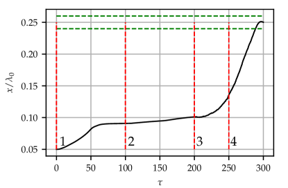
(a)

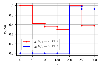
(b)

Figure 6: The trajectory of the bubble controlled by the RL agent (top panel) and the chosen pressure amplitude values (bottom panel).

To verify the actions of the agent, 2-dimensional parameter studies were carried out in the parameter space of the pressure amplitudes via GPU-accelerated initial value problem computations to directly search the optimal pressure amplitude combinations. The applied solver was written in Python and using the numba library that supports writing CUDA kernels [44]. The implemented algorithm is the fourth-order Runga-Kutta-Cash-Karp method with fifth-order error estimation. At every pressure amplitude combination, numerical simulations were carried out over 50 acoustic cycles (one time-step) and the averaged translational velocity was calculated. During the computations, the absolute and relative tolerance were set to $10^{-10}$. These parameter maps were calculated along the trajectory given in the top panel of Fig. 6 at bubble positions labelled from 1 to 4 and marked with vertical red dashed lines. The results are given in Figure 7. The resolution of each parameter map is $P_{A0}\times P_{A1}=256\times 256$. The black dots denote the maximum velocity. The parameters chosen by the agent are plotted with green dots.

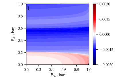
(a)

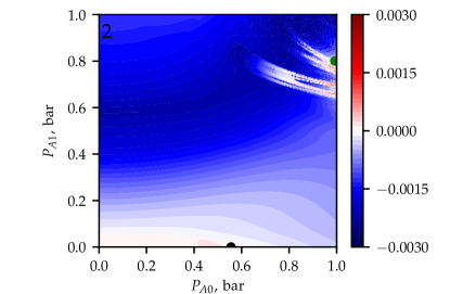
(b)

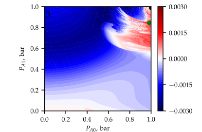
(c)

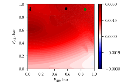
(d)

Figure 7: The averaged translational velocity over 50 acoustic periods as a function of the pressure amplitude components. The black dots denote the optimal parameter set obtained by the direct search for the maximum velocity and the green dots denote the parameter set chosen by the RL agent.

In the first step, the direct search and agent suggest the same action that results in maximal displacement. In the second case, the direct search suggests an optimal parameter set at ($P_{A0}=1\,\mathrm{bar}$ and $P_{A1}=0.8\,\mathrm{bar}$). Although it results in a higher displacement compared to the trajectory obtained by the RL, this narrow domain requires an overly precise amplitude setting that may be infeasible in practice. The RL chose a more robust decision compared to the direct search. As the bubble moves towards the positive direction, the domain resulting in a high translational velocity increases. Thus; in the third case, the agent picks a parameter set from this domain. Lastly, the agent picks an action that results in an accurate final position.

5 Conclusion

The present paper proposes that reinforcement learning (RL) can be a powerful tool in developing controllers to manipulate bubble clusters (e.g., minimising attenuation via manipulating bubble positions to keep an optimal structure). To demonstrate this a simple but non-trivial case is investigated, where the task of the agent was to control a single bubble on the shortest path from any random position to the target position. In our study, the target position was randomized. However, depending on the applications, the target position can be specified, e.g., the best spot of chemical activity [53, 54, 7], or in the case of ultrasonic water treatment [55, 56, 57, 58] or clot lysis [59, 60] the bubble may be driven near specific surfaces. It is worthwhile to mention that the agent was rewarded only for the minimization of the distance, which implicitly encouraged the agent to seek fast position control. A fine-tuned reward function allows encoding additional constraints such as minimization of the consumed energy [61, 62, 63, 64] or avoiding bubble break-off due to surface instabilities [65, 66, 67, 68, 69, 70, 71, 72, 73] via adding penalties or the maximization of various chemical products [74, 75, 76, 2, 77, 78, 79].

The RL agent was capable of finding optimal control on a wide range of initial positions that move the bubble to an arbitrary target position within the shortest amount of time. For example, in the case presented in Fig. 6, the naive approach (pushing the bubble with the primary Bjerknes force) would require 2150 acoustic periods, which is 7.2 times higher than the solution of the RL. It was capable of developing non-trivial solutions, see Fig. 5. In the lower right domain, the bubble is moved from the stable antinode close to the unstable node ($x/\lambda=0.05$). That direction of movement can not be justified by the linear theory of translational bubble motion (see again Fig. 2).

The structural similarities of parameter maps observed in our previous paper [43] imply that the size of the bubble $R_{0}$ determines the proper choice of the $f_{0}$, and $f_{1}$ frequency components. To develop universal control one can extend the observation vector with an equilibrium bubble size and apply for example parameterized action space [80, 81, 82], such as $a=[(f_{0},f_{1})_{k},(P_{A0},P_{A1})_{k}]$, where $(f_{0},f_{1})_{k}\in[(f_{0},f_{1})_{1},(f_{0},f_{1})_{2}...(f_{0},f_{1})_{K}]$ is a discrete frequency combination (assuming standing waves) and $(P_{A0},P_{A1})_{k}$ is its parameter vector. The investigation of such cases was beyond the scope of the present paper.

The high-resolution simulations revealed that by precise parameter tuning, better trajectories can be found via direct numeric solutions. However, implementing real-time controllers, for more complex problems, may be infeasible due to the increasing computational time. The computational time of a single parameter map plotted in Fig. 7 is approximately 4-5 seconds on a GeForce GTX 1070 Graphics card. The applied GPU-accelerated solver has a similar computation performance as the MPGOS [83, 84] program package (not shown here). On the contrary, the inference time of the neural network (policy) is approximately $1.2\,\mathrm{ms}$ on the same GPU (including the data transfer between host and device). The computation time of the direct search method scales unfavourably by the increasing complexity, e.g., adding a secondary bubble compared to the network inference.

The increasing complexity of the problem (e.g., multi-frequency driving [34], extension to bubble cluster [85, 86, 87, 88, 89, 90]) requires more sophisticated reinforcement learning algorithms, that allow the sufficient exploration of the state and action space. One promising candidate is Proximal Policy Optimization (PPO) [91], known for its scalability using vectorized environments allowing efficient parallelization [92, 93] and improved sample efficiency in training.

Declaration of Competing Interest

The authors declare that they have no known competing financial interests or personal relationships that could have appeared to influence the work reported in this paper.

References

- [1] K. Yasui, Acoustic Cavitation and Bubble Dynamics, Springer International Publishing, Cham, 2018, Ch. Bubble Dynamics, pp. 37–97.
- [2] H. Xu, B. W. Zeiger, K. S. Suslick, Sonochemical synthesis of nanomaterials, Chem. Soc. Rev. 42 (7) (2013) 2555–2567.
- [3] T. Sivasankar, V. S. Moholkar, Mechanistic approach to intensification of sonochemical degradation of phenol, Chem. Eng. J. 149 (1) (2009) 57 – 69.
- [4] T. Sivasankar, V. S. Moholkar, Physical insights into the sonochemical degradation of recalcitrant organic pollutants with cavitation bubble dynamics, Ultrason. Sonochem. 16 (6) (2009) 769 – 781.
- [5] V. L. Gole, A. Fishgold, R. Sierra-Alvarez, P. Deymier, M. Keswani, Treatment of perfluorooctane sulfonic acid (pfos) using a large-scale sonochemical reactor, Sep. Purif. Technol 194 (2018) 104–110.
- [6] A. A. Pradhan, P. R. Gogate, Degradation of p-nitrophenol using acoustic cavitation and Fenton chemistry, J. Hazard. Mater. 173 (1) (2010) 517–522.
- [7] A. Gedanken, Using sonochemistry for the fabrication of nanomaterials, Ultrason. Sonochem. 11 (2) (2004) 47–55.
- [8] V. S. Sutkar, P. R. Gogate, Design aspects of sonochemical reactors: Techniques for understanding cavitational activity distribution and effect of operating parameters, Chem. Eng. J. 155 (1) (2009) 26–36.
- [9] M. M. van Iersel, N. E. Benes, J. T. Keurentjes, Importance of acoustic shielding in sonochemistry, Ultrason. Sonochem. 15 (4) (2008) 294–300.
- [10] A. J. Sojahrood, Q. Li, H. Haghi, R. Karshafian, T. M. Porter, M. C. Kolios, Effect of ultrasound pressure and bubble-bubble interaction on the nonlinear attenuation and sound speed in a bubbly medium, J. Acoust. Soc. Am. 141 (5) (2017) 3741–3741.
- [11] Y. Sriphutkiat, Y. Zhou, Particle manipulation using standing acoustic waves in the microchannel at dual-frequency excitation: Effect of power ratio, Sens. Actuators A: Phys. 263 (2017) 521–529.
- [12] O. Dron, J.-L. Aider, Varying the agglomeration position of particles in a micro-channel using acoustic radiation force beyond the resonance condition, Ultrasonics 53 (7) (2013) 1280–1287.
- [13] M. Kandemir, M. Beelen, R. Wagterveld, D. Yntema, K. Keesman, Dynamic acoustic fields for size selective particle separation on centimeter scale, Journal of Sound and Vibration 490 (2021) 115723.
- [14] K. Latifi, A. Kopitca, Q. Zhou, Model-free control for dynamic-field acoustic manipulation using reinforcement learning, IEEE Access 8 (2020) 20597–20606.
- [15] G. Vuillermet, P.-Y. Gires, F. Casset, C. Poulain, Chladni patterns in a liquid at microscale, Phys. Rev. Lett. 116 (2016) 184501.
- [16] J. Goldowsky, M. Mastrangeli, L. Jacot-Descombes, M. R. Gullo, G. Mermoud, J. Brugger, A. Martinoli, B. J. Nelson, H. F. Knapp, Acousto-fluidic system assisting in-liquid self-assembly of microcomponents, J Micromech Microeng 23 (12) (2013) 125026.
- [17] K. Maeda, A. D. Maxwell, Controlling the dynamics of cloud cavitation bubbles through acoustic feedback, Phys. Rev. Applied 15 (2021) 034033.
- [18] J. Lee, M. Ashokkumar, K. Yasui, T. Tuziuti, T. Kozuka, A. Towata, Y. Iida, Development and optimization of acoustic bubble structures at high frequencies, Ultrason. Sonochem. 18 (1) (2011) 92–98.
- [19] J. Rosselló, D. Dellavale, F. Bonetto, Positional stability and radial dynamics of sonoluminescent bubbles under bi-harmonic driving: Effect of the high-frequency component and its relative phase, Ultrason. Sonochem. 31 (2016) 610–625.
- [20] J. Rosselló, D. Dellavale, F. Bonetto, Stable tridimensional bubble clusters in multi-bubble sonoluminescence (mbsl), Ultrason. Sonochem. 22 (2015) 59–69.
- [21] Y. Abe, M. Kawaji, T. Watanabe, Study on the bubble motion control by ultrasonic wave, Exp. Therm. Fluid Sci. 26 (6) (2002) 817–826.
- [22] C. C. Mei, X. Zhou, Parametric resonance of a spherical bubble, J. Fluid Mech. 229 (1991) 29–50.
- [23] Z. C. Feng, L. G. Leal, Translational instability of a bubble undergoing shape oscillations, Phys. Fluids 7 (6) (1995) 1325–1336.
- [24] A. A. Doinikov, Translational motion of a bubble undergoing shape oscillations, J. Fluid Mech. 501 (2004) 1–24.
- [25] R. Mettin, A. A. Doinikov, Translational instability of a spherical bubble in a standing ultrasound wave, Appl. Acoust. 70 (10) (2009) 1330 – 1339.
- [26] M. Versluis, D. E. Goertz, P. Palanchon, I. L. Heitman, S. M. van der Meer, B. Dollet, N. de Jong, D. Lohse, Microbubble shape oscillations excited through ultrasonic parametric driving, Phys. Rev. E 82 (2) (2010) 026321.
- [27] L. Bai, W. Xu, J. Deng, C. Li, D. Xu, Y. Gao, Generation and control of acoustic cavitation structure, Ultrason. Sonochem. 21 (5) (2014) 1696–1706.
- [28] R. S. Sutton, A. G. Barto, Reinforcement Learning: An Introduction, MIT Press, 2018.
- [29] H. Jean-François, M. Mangassarian, P. S. Kumaran, Markov Decision Processes: Concepts and Algorithms, Wiley-IEEE Press, 2003.
- [30] V. Mnih, K. Kavukcuoglu, D. Silver, et al., Playing atari with deep reinforcement learning, arXiv preprint arXiv:1312.5602.
- [31] V. Mnih, et al., Human-level control through deep reinforcement learning, Nature.
- [32] T. P. Lillicrap, et al., Continuous control with deep reinforcement learning, arXiv preprint arXiv:1509.02971.
- [33] P. A. Tatake, A. B. Pandit, Modelling and experimental investigation into cavity dynamics and cavitational yield: influence of dual frequency ultrasound sources, Chem. Eng. Sci. 57 (22) (2002) 4987–4995.
- [34] D. Suo, B. Govind, S. Zhang, Y. Jing, Numerical investigation of the inertial cavitation threshold under multi-frequency ultrasound, Ultrason. Sonochem. 41 (2018) 419–426.
- [35] Y. Zhang, Y. Zhang, S. Li, The secondary bjerknes force between two gas bubbles under dual-frequency acoustic excitation, Ultrason. Sonochem. 29 (2016) 129–145.
- [36] Y. Zhang, Y. Zhang, S. Li, Combination and simultaneous resonances of gas bubbles oscillating in liquids under dual-frequency acoustic excitation, Ultrason. Sonochem. 35 (2017) 431–439.
- [37] Y. Zhang, D. Billson, S. Li, Influences of pressure amplitudes and frequencies of dual-frequency acoustic excitation on the mass transfer across interfaces of gas bubbles, Int. J. Heat Mass Transf. 66 (2015) 16–20.
- [38] A. A. Doinikov, Translational motion of a spherical bubble in an acoustic standing wave of high intensity, Phys. Fluids 14 (4) (2002) 1420–1425.
- [39] J. B. Keller, M. Miksis, Bubble oscillations of large amplitude, J. Acoust. Soc. Am. 68 (2) (1980) 628–633.
- [40] A. A. Doinikov, Bjerknes forces and translational bubble dynamics, Bubble and particle dynamics in acoustic fields: modern trends and applications 661 (2005) 95–143.
- [41] L. A. Crum, Bjerknes forces on bubbles in a stationary sound field, J. Acoust. Soc. Am. 57 (6) (1975) 1363–1370.
- [42] V. Levich, Physicochemical Hydrodynamics, 2nd Edition, Prentice–Hall, Englewood Cliffs, NJ, 1962.
- [43] K. Klapcsik, F. Hegedűs, Numerical investigation of the translational motion of bubbles: The comparison of capabilities of the time-resolved and the time-averaged methods, Ultrason. Sonochem. 92 (2023) 106253.
-
[44]
N. Community, Numba Documentation, Anaconda,
Inc. (2022).
URL https://numba.pydata.org/ - [45] G. Brockman, V. Cheung, L. Pettersson, J. Schneider, J. Schulman, J. Tang, W. Zaremba, OpenAI Gym, https://github.com/openai/gym (2016).
- [46] D. Silver, G. Lever, N. Heess, T. Degris, D. Wierstra, M. Riedmiller, Deterministic policy gradient algorithms, in: International conference on machine learning, Pmlr, 2014, pp. 387–395.
- [47] A. Paszke, S. Gross, F. Massa, A. Lerer, J. Bradbury, G. Chanan, T. Killeen, Z. Lin, N. Gimelshein, L. Antiga, A. Desmaison, A. Köpf, E. Yang, Z. DeVito, M. Raison, A. Tejani, S. Chilamkurthy, B. Steiner, L. Fang, J. Bai, S. Chintala, Pytorch: An imperative style, high-performance deep learning library (2019). arXiv:1912.01703.
- [48] Y. Gao, et al., Cleanrl: A clean implementation for deep reinforcement learning, arXiv preprint arXiv:1910.07207.
- [49] R. Mettin, I. Akhatov, U. Parlitz, C. D. Ohl, W. Lauterborn, Bjerknes forces between small cavitation bubbles in a strong acoustic field, Phys. Rev. E 56 (3) (1997) 2924–2931.
- [50] T. J. Matula, S. M. Cordry, R. A. Roy, L. A. Crum, Bjerknes force and bubble levitation under single-bubble sonoluminescence conditions, J. Acoust. Soc. Am. 102 (3) (1997) 1522–1527.
- [51] I. Akhatov, R. Mettin, C. D. Ohl, U. Parlitz, W. Lauterborn, Bjerknes force threshold for stable single bubble sonoluminescence, Phys. Rev. E 55 (1997) 3747–3750.
- [52] O. Louisnard, Analytical expressions for primary Bjerknes force on inertial cavitation bubbles, Phys. Rev. E 78 (3) (2008) 036322.
- [53] M. H. Islam, M. T. Y. Paul, O. S. Burheim, B. G. Pollet, Recent developments in the sonoelectrochemical synthesis of nanomaterials, Ultrason. Sonochem. 59 (2019) 104711.
- [54] S. S. Rashwan, I. Dincer, A. Mohany, B. G. Pollet, The Sono-Hydro-Gen process (Ultrasound induced hydrogen production): Challenges and opportunities, Int. J. Hydrog. Energy. 44 (29) (2019) 14500–14526.
- [55] J. González-García, V. Sáez, I. Tudela, M. I. Díez-Garcia, M. Deseada Esclapez, O. Louisnard, Sonochemical treatment of water polluted by chlorinated organocompounds. a review, Water 2 (1) (2010) 28–74.
- [56] M. Esclapez, V. Sáez, D. Milán-Yáñez, I. Tudela, O. Louisnard, J. González-García, Sonoelectrochemical treatment of water polluted with trichloroacetic acid: From sonovoltammetry to pre-pilot plant scale, Ultrason. Sonoch. 17 (6) (2010) 1010–1020.
- [57] M. Zupanc, T. Kosjek, M. Petkovšek, M. Dular, B. Kompare, B. Širok, Željko Blažeka, E. Heath, Removal of pharmaceuticals from wastewater by biological processes, hydrodynamic cavitation and uv treatment, Ultrason. Sonochem. 20 (4) (2013) 1104–1112.
- [58] M. Dular, T. Griessler-Bulc, I. Gutierrez-Aguirre, E. Heath, T. Kosjek, A. Krivograd Klemenčič, M. Oder, M. Petkovšek, N. Rački, M. Ravnikar, A. Šarc, B. Širok, M. Zupanc, M. Žitnik, B. Kompare, Use of hydrodynamic cavitation in (waste)water treatment, Ultrason. Sonochem. 29 (2016) 577–588.
- [59] K. B. Bader, M. J. Gruber, C. K. Holland, Shaken and stirred: Mechanisms of ultrasound-enhanced thrombolysis, Ultrasound Med. Biol 41 (1) (2015) 187–196.
- [60] C. Acconcia, B. Y. C. Leung, K. Hynynen, D. E. Goertz, Interactions between ultrasound stimulated microbubbles and fibrin clots, Appl. Phys. Lett. 103 (5) (2013) 053701.
- [61] A. Sojahrood, H. Haghi, Q. Li, T. Porter, R. Karshafian, M. Kolios, Nonlinear power loss in the oscillations of coated and uncoated bubbles: Role of thermal, radiation and encapsulating shell damping at various excitation pressures, Ultrasos. Sonochem. 66 (2020) 105070.
- [62] A. Sojahrood, H. Haghi, R. Karshafian, M. Kolios, Critical corrections to models of nonlinear power dissipation of ultrasonically excited bubbles, Ultrason. Sonochem. 66 (2020) 105089.
- [63] A. Sojahrood, H. Haghi, R. Karshafian, M. Kolios, Nonlinear dynamics and bifurcation structure of ultrasonically excited lipid coated microbubbles, Ultrason. Sonochem. 72 (2021) 105405.
- [64] A. J. Sojahrood, H. Haghi, R. Karshafian, M. C. Kolios, Classification of the major nonlinear regimes of oscillations, oscillation properties, and mechanisms of wave energy dissipation in the nonlinear oscillations of coated and uncoated bubbles, Phys. Fluids 33 (1) (2021) 016105.
- [65] M. P. Brenner, D. Lohse, T. F. Dupont, Bubble shape oscillations and the onset of sonoluminescence, Phys. Rev. Lett. 75 (5) (1995) 954–957.
- [66] V. A. Bogoyavlenskiy, Single-bubble sonoluminescence: Shape stability analysis of collapse dynamics in a semianalytical approach, Phys. Rev. E 62 (2) (2000) 2158–2167.
- [67] B. Dollet, S. M. van der Meer, V. Garbin, N. de Jong, D. Lohse, M. Versluis, Nonspherical oscillations of ultrasound contrast agent microbubbles, Ultrasound Med. Biol. 34 (9) (2008) 1465–1473.
- [68] Y. Hao, A. Prosperetti, The effect of viscosity on the spherical stability of oscillating gas bubbles, Phys. Fluids 11 (6) (1999) 1309–1317.
- [69] J. Holzfuss, Surface-wave instabilities, period doubling, and an approximate universal boundary of bubble stability at the upper threshold of sonoluminescence, Phys. Rev. E 77 (6) (2008) 066309.
- [70] B. Lalanne, N. A. Chebel, J. Vejražka, S. Tanguy, O. Masbernat, F. Risso, Non-linear shape oscillations of rising drops and bubbles: Experiments and simulations, Phys. Fluids 27 (12) (2015) 123305.
- [71] S. J. Shaw, Translation and oscillation of a bubble under axisymmetric deformation, Phys. Fluids 18 (7) (2006) 072104.
- [72] S. J. Shaw, The stability of a bubble in a weakly viscous liquid subject to an acoustic traveling wave, Phys. Fluids 21 (2) (2009) 022104.
- [73] S. J. Shaw, Nonspherical sub-millimeter gas bubble oscillations: Parametric forcing and nonlinear shape mode coupling, Phys. Fluids 29 (12) (2017) 122103.
- [74] M. H. Islam, O. S. Burheim, J.-Y. Hihn, B. Pollet, Sonochemical conversion of \chCO2 into hydrocarbons: The sabatier reaction at ambient conditions, Ultrason. Sonochem. 73 (2021) 105474.
- [75] R. Pflieger, T. Chave, G. Vite, L. Jouve, S. I. Nikitenko, Effect of operational conditions on sonoluminescence and kinetics of \chH2O2 formation during the sonolysis of water in the presence of \chAr/\chO2 gas mixture, Ultrason. Sonochem. 26 (2015) 169–175.
- [76] T. Ouerhani, R. Pflieger, W. Ben Messaoud, S. I. Nikitenko, Spectroscopy of sonoluminescence and sonochemistry in water saturated with \chN2–\chAr mixtures, J. Phys. Chem. B 119 (52) (2015) 15885–15891.
- [77] M. H. Islam, O. S. Burheim, B. G. Pollet, Sonochemical and sonoelectrochemical production of hydrogen, Ultrason. Sonochem. 51 (2019) 533–555.
- [78] S. Merouani, O. Hamdaoui, Y. Rezgui, M. Guemini, Mechanism of the sonochemical production of hydrogen, Int. J. Hydrog. Energy. 40 (11) (2015) 4056–4064.
- [79] K. Kerboua, O. Hamdaoui, Sonochemical production of hydrogen: Enhancement by summed harmonics excitation, Chem. Phys. 519 (2019) 27–37.
- [80] W. Masson, P. Ranchod, G. Konidaris, Reinforcement learning with parameterized actions (2015). arXiv:1509.01644.
- [81] O. Delalleau, M. Peter, E. Alonso, A. Logut, Discrete and continuous action representation for practical rl in video games (2019). arXiv:1912.11077.
- [82] Z. Fan, R. Su, W. Zhang, Y. Yu, Hybrid actor-critic reinforcement learning in parameterized action space (2019). arXiv:1903.01344.
- [83] https://github.com/ferenchegedus/massively-parallel-gpu-ode-solver.
- [84] F. Hegedűs, MPGOS: GPU accelerated integrator for large number of independent ordinary differential equation systems, Budapest University of Technology and Economics, Budapest, Hungary (2019).
- [85] A. A. Doinikov, Mathematical model for collective bubble dynamics in strong ultrasound fields, J. Acoust. Soc. Am. 116 (2) (2004) 821–827.
- [86] R. Mettin, From a single bubble to bubble structures in acoustic cavitation, in: Oscillations, Waves and Interactions: Sixty Years Drittes Physikalisches Institut ; a Festschrift, Universitätsverlag Göttingen, Göttingen, Germany, 2007, pp. 171–198.
- [87] R. Mettin, Bubble structures in acoustic cavitation, in: Bubble and Particle Dynamics in Acoustic Fields: Modern Trends and Applications, Research Signpost, Trivandrum, Kerala, India, 2005, pp. 1–36.
- [88] R. Mettin, S. Luther, C.-D. Ohl, W. Lauterborn, Acoustic cavitation structures and simulations by a particle model, Ultrason. Sonochem. 6 (1) (1999) 25–29.
- [89] R. Mettin, C.-D. Ohl, W. Lauterborn, Particle approach to structure formation in acoustic cavitation, in: L. A. Crum, T. J. Mason, J. L. Reisse, K. S. Suslick (Eds.), Sonochemistry and Sonoluminescence, Springer Netherlands, Dordrecht, 1999, pp. 139–144.
- [90] P. Koch, D. Krefting, R. Mettin, W. Lauterborn, Simulation of the translational motion of few cavitation bubbles in an ultrasonic field, in: IEEE Symposium on Ultrasonics, 2003, Vol. 2, 2003, pp. 1475–1478 Vol.2.
- [91] J. Schulman, et al., Proximal policy optimization algorithms, arXiv preprint arXiv:1707.06347.
- [92] N. Heess, D. TB, S. Sriram, J. Lemmon, J. Merel, G. Wayne, Y. Tassa, T. Erez, Z. Wang, S. M. A. Eslami, M. Riedmiller, D. Silver, Emergence of locomotion behaviours in rich environments (2017). arXiv:1707.02286.
- [93] N. Rudin, D. Hoeller, P. Reist, M. Hutter, Learning to walk in minutes using massively parallel deep reinforcement learning (2022). arXiv:2109.11978.