Modeling Homophily in Exponential-Family Random Graph Models for Bipartite Networks

Abstract

Homophily, the tendency of individuals who are alike to form ties with one another, is an important concept in the study of social networks. Yet accounting for homophily effects is complicated in the context of bipartite networks where ties connect individuals not with one another but rather with a separate set of nodes, which might also be individuals but which are often an entirely different type of objects. As a result, much work on the effect of homophily in a bipartite network proceeds by first eliminating the bipartite structure, collapsing a two-mode network to a one-mode network and thereby ignoring potentially meaningful structure in the data. We introduce a set of methods to model homophily on bipartite networks without losing information in this way, then we demonstrate that these methods allow for substantively interesting findings in management science not possible using standard techniques. These methods are implemented in the widely-used ergm package for R.

, and

1 Introduction and Motivation

Networks are an increasingly popular method for capturing patterns of interactions among pairs, or more generally sets, of individuals. In its most basic form, a network consists of a fixed set of nodes, also called vertices, along with a set of pairs of those nodes. Each pair is called a tie, or an edge, and may be thought of as connecting the two nodes by a particular relationship whose definition depends on the application. Relationships in networks are often thought to be influenced by partner selection mechanisms. One of the most popular partner selection mechanisms is called homophily, the basic idea of which is that ties are more likely to form between individuals who match on one or more attributes. This partner selection mechanism then regularly leads to the formation of homogeneous groups. The importance of homophily is well-established both in academia, as is evident by the literature in different fields of the social sciences (McPherson, Smith-Lovin and Cook, 2001; Ertug et al., 2022), as well as outside of academia, as is reflected by the well-known proverb “birds of a feather flock together.” It is no surprise, then, that its incorporation into statistical models for social networks is often straightforward.

Yet dealing with homophily is not straightforward for bipartite networks, also known as affiliation or two-mode networks. Technically, a bipartite network consists of two disjoint sets, or modes, of vertices, $V_{1}$ and $V_{2}$, and a set of edges $E\subseteq V_{1}\times V_{2}$. That is, every edge must link a vertex from mode 1 to a vertex from mode 2. in layman’s terms, “actors” comprising one mode of a bipartite network are affiliated with “events” of its second mode, so connections among actors arise only indirectly through joint affiliations to events and vice versa. As there are multiple types of two-mode networks where the terms “actor” and “event” do not accurately describe vertices, we simply refer to them as “mode 1” and “mode 2”. In cases in which bipartite networks are composed of modes of the same node type—for instance, in a heterosexual contact network where partnerships only occur between opposite-gender nodes—homophily involving, say, age category or race may be considered as in the standard, non-bipartite case. Such a composition, however, is rare. Typically, the two modes of nodes are comprised of entirely different types of entities, and homophily is only theoretically meaningful among entities of the same type. It is these latter cases in which the current article is relevant.

As an example of the potential complexity of homophily in two-mode networks, consider the case of corporate boards, in which directors (mode 2) are affiliated with companies (mode 1). Interlocking directorates, which occur “when a person affiliated with one organization sits on the board of directors of another organization” (Mizruchi, 1996), are studied by scholars from various disciplines, such as sociology (Chu and Davis, 2016) or management research (Lamb and Roundy, 2016; Martin, Gözübüyük and Becerra, 2015). Here, researchers may take on a resource dependency perspective (Pfeffer and Salancik, 2003) and consequently raise questions about the role of industry homophily, estimating whether directors are more likely to sit on the boards of firms that belong to the same industry rather than distinct industries. Yet different conceptions of how to measure the strength of homophily can give rise to different statistics. It is a fundamental theoretical difference if homophily is estimated (a) by counting through how many directors a focal firm is connected to another homophilous firm, or (b) by counting to how many different homophilous firms a director connects a focal firm. These perspectives represent a node-centric and an edge-centric view, respectively. If these counts are totaled for the entire network, the two views produce equivalent homophily statistics, and a straightforward approach does not distinguish between them.

This paper introduces a method to put either the node- or edge-centric perspective into focus and estimate homophily via a statistic that is nonlinear in, respectively, the number of paths between a given homophilous node pair or the number of edges that complete paths with homophilous endpoints starting with a given edge. This method allows for a deeper integration of social science theories and network models while providing mathematical flexibility that can lead to improved modeling performance.

We present two applications that illustrate the relevance of this method to various disciplines prone to social network analysis, such as sociology, management research, and social psychology. Our results suggest that the reformulated homophily effects we introduce to the analysis of two-mode networks allow researchers from various fields to find nuanced answers to contemporary questions.

The first application is a dataset collected among members of an organization in which subjects listed their core competencies. We show that using the node-centric reformulation not only improves model fit as measured by log-likelihood, but produces estimates that allow for meaningful interpretation regarding the distribution of hard and soft skills (such as financial analysis versus planning) in an organization, adding to ongoing scholarly discussions and creating implications for practitioners (Laker and Powell, 2011; Robles, 2012).

The second application refers to the aforementioned directorates. Analyzing the network of boards of directors among the Fortune 500, we argue that in this dataset, the role of gender is best captured by making use of the edge-centric reformulation of two-mode homophily. Our results indicate that in addition to the proverbial glass ceiling, i.e., the difficulty faced by females in ascending the corporate ladder as evidenced by the fact that only 32% of board members are female, there may be a “glass door” that moderates females’ horizontal integration into the corporate elite. These findings add to ongoing debates about the role of demographic attributes in social elite cohesion and corporate governance (Zhu and Westphal, 2014; McDonald and Westphal, 2013; Park and Westphal, 2013).

Both of these applications are examined in Section 4. First, we establish the statistical foundation, which is based on a modeling framework known as exponential-family random graph models, or ERGMs. Section 2 discusses particular complications of modeling relationships in a bipartite network and describes the ERGM framework. Section 3 introduces novel modeling tools within the ERGM framework, explaining their favorable theoretical properties from both a statistical and application-specific perspective. Section 5 offers some concluding remarks, while Appendices A and B provide additional theoretical material regarding the use of these methods in an ERGM framework.

2 Bipartite Networks and Exponential-Family Random Graph Models

Basic notions of analyzing bipartite networks are reviewed by Borgatti and Everett (1997), who explain how many familiar network techniques and measurements—e.g., visualization of networks, nodal degree, network density, betweenness and centrality—may be extended to the bipartite case. Latapy, Magnien and Vecchio (2008) cite numerous applications of two-mode networks and similarly extend additional common notions, introducing statistics like the “redundancy coefficient” or expanding on others such as the bipartite clustering coefficient of Robins and Alexander (2004).

When the modeling goal is to understand relationships among nodes belonging to just one of the two modes, as is the case when studying homophily, a commonly-used technique is to project from a two-mode network onto either of the two modes. Here, we explain projections and introduce the modeling framework of exponential-family random graph models, or ERGMs.

2.1 Projections onto one-mode networks

Any two-mode network gives rise to two separate one-mode projections, as illustrated by Figure 1. The edges in the projections can include weights, indicating the number of distinct nodes of the opposite mode that connect to a given node pair. To consider homophily, we might apply standard modeling techniques, such as those presented in Section 2.2, to either of the projections.

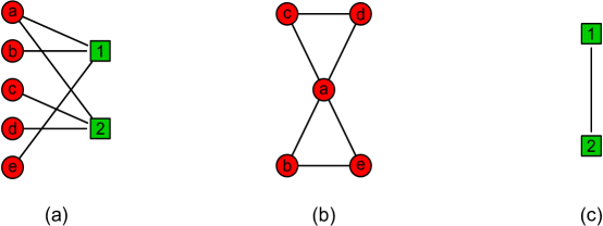
Figure 1: Networks (b) and (c) depict the projections of the original two-mode network (a) onto mode 1 nodes (circles) and mode 2 nodes (squares), respectively. An edge between a pair of nodes exists in the projection if and only if there is at least one two-path between those two nodes in (a).

Yet as Latapy, Magnien and Vecchio (2008) point out, the projection approach is not ideal for several reasons: In brief, the projection loses information about the original bipartite structure of the network, and it may even distort certain types of information such as clustering coefficients. For instance, in the interlocking directorates example cited in Section 1, projecting the underlying two-mode structure onto one-mode networks that depict connections between firms (Withers, Howard and Tihanyi, 2020; Howard, Withers and Tihanyi, 2017) loses information about attributes on the director level is almost lost in its entirety. Similarly, while there are various studies about the role of director-level attributes, the network context in which corporate directors maneuver is typically neglected (Westphal and Stern, 2007; McDonald and Westphal, 2013).

For bipartite networks, we let $n=n_{1}+n_{2}$, where nodes 1 through $n_{1}$ are of mode 1 and nodes $n_{1}+1$ through $n$ are of mode 2. We denote a random network by the $n\times n$ matrix $\mathbf{\textstyle}\bf Y$, where $Y_{ij}$ equals 0 or 1 according to whether the $(i,j)$th edge is absent or present. In this case, $\mathbf{\textstyle}\bf Y$ may only have nonzero entries in the off-diagonal rectangular submatrix in rows 1 to $n_{1}$ and columns $n_{1}+1$ to $n$, along with its mirror image since $\mathbf{\textstyle}\bf Y$ is usually symmetric in a bipartite setting. The matrix $\mathchoice{\mbox{$\mathbf{\displaystyle}\bf Y$}}{\mbox{$\mathbf{\textstyle}\bf Y$}}{\mbox{$\mathbf{\scriptstyle}\bf Y$}}{\mbox{$\mathbf{\scriptscriptstyle}\bf Y$}}^{2}$ contains both projection networks from Figure 1(b) and (c), with the mode 1 projection in the upper-left $n_{1}\times n_{1}$ submatrix and the mode 2 projection in the lower-right $n_{2}\times n_{2}$ submatrix. Each entry in these submatrices gives the number of distinct paths of length two connecting the two nodes indexed by the row and column numbers of the entry; in particular, nonzero entries of $\mathchoice{\mbox{$\mathbf{\displaystyle}\bf Y$}}{\mbox{$\mathbf{\textstyle}\bf Y$}}{\mbox{$\mathbf{\scriptstyle}\bf Y$}}{\mbox{$\mathbf{\scriptscriptstyle}\bf Y$}}^{2}$ indicate edges in one of the projection networks.

2.2 Exponential-family Random Graph Models

The aim of this article is to model the nonzero elements of $\mathbf{\textstyle}\bf Y$ itself rather than $\mathchoice{\mbox{$\mathbf{\displaystyle}\bf Y$}}{\mbox{$\mathbf{\textstyle}\bf Y$}}{\mbox{$\mathbf{\scriptstyle}\bf Y$}}{\mbox{$\mathbf{\scriptscriptstyle}\bf Y$}}^{2}$, and for this purpose we turn to the family of probability models known as exponential-family random graph models (ERGMs). Robins et al. (2007a) give a general introduction to these models, which are sometimes called p-star models in reference to the seminal paper of Wasserman and Pattison (1996). These models define a parametric family of probability distributions on the space of all possible networks. The basic ERGM may be written

$$P_{\theta}(\mathchoice{\mbox{$\mathbf{\displaystyle}\bf Y$}}{\mbox{$\mathbf{\textstyle}\bf Y$}}{\mbox{$\mathbf{\scriptstyle}\bf Y$}}{\mbox{$\mathbf{\scriptscriptstyle}\bf Y$}}=\mathchoice{\mbox{$\mathbf{\displaystyle}\bf y$}}{\mbox{$\mathbf{\textstyle}\bf y$}}{\mbox{$\mathbf{\scriptstyle}\bf y$}}{\mbox{$\mathbf{\scriptscriptstyle}\bf y$}})=\frac{\exp\{\sum_{i=1}^{p}\theta_{i}s_{i}(\mathchoice{\mbox{$\mathbf{\displaystyle}\bf y$}}{\mbox{$\mathbf{\textstyle}\bf y$}}{\mbox{$\mathbf{\scriptstyle}\bf y$}}{\mbox{$\mathbf{\scriptscriptstyle}\bf y$}})\}}{\kappa(\mathchoice{\mbox{$\mathbf{\displaystyle}\bf\theta$}}{\mbox{$\mathbf{\textstyle}\bf\theta$}}{\mbox{$\mathbf{\scriptstyle}\bf\theta$}}{\mbox{$\mathbf{\scriptscriptstyle}\bf\theta$}})},\quad\mathchoice{\mbox{$\mathbf{\displaystyle}\bf y$}}{\mbox{$\mathbf{\textstyle}\bf y$}}{\mbox{$\mathbf{\scriptstyle}\bf y$}}{\mbox{$\mathbf{\scriptscriptstyle}\bf y$}}\in{\cal Y},$$ (1)

where $s_{1}(\mathchoice{\mbox{$\mathbf{\displaystyle}\bf y$}}{\mbox{$\mathbf{\textstyle}\bf y$}}{\mbox{$\mathbf{\scriptstyle}\bf y$}}{\mbox{$\mathbf{\scriptscriptstyle}\bf y$}}),\ldots,s_{p}(\mathchoice{\mbox{$\mathbf{\displaystyle}\bf y$}}{\mbox{$\mathbf{\textstyle}\bf y$}}{\mbox{$\mathbf{\scriptstyle}\bf y$}}{\mbox{$\mathbf{\scriptscriptstyle}\bf y$}})$ are user-defined statistics measured on the network $\mathbf{\textstyle}\bf y$ and we denote the vector of all network statistics by $\mathchoice{\mbox{$\mathbf{\displaystyle}\bf s$}}{\mbox{$\mathbf{\textstyle}\bf s$}}{\mbox{$\mathbf{\scriptstyle}\bf s$}}{\mbox{$\mathbf{\scriptscriptstyle}\bf s$}}(\mathchoice{\mbox{$\mathbf{\displaystyle}\bf y$}}{\mbox{$\mathbf{\textstyle}\bf y$}}{\mbox{$\mathbf{\scriptstyle}\bf y$}}{\mbox{$\mathbf{\scriptscriptstyle}\bf y$}})$. When covariates $X$ should be included in the model, we may add $X$ to the notation and write $\mathchoice{\mbox{$\mathbf{\displaystyle}\bf s$}}{\mbox{$\mathbf{\textstyle}\bf s$}}{\mbox{$\mathbf{\scriptstyle}\bf s$}}{\mbox{$\mathbf{\scriptscriptstyle}\bf s$}}(\mathchoice{\mbox{$\mathbf{\displaystyle}\bf y$}}{\mbox{$\mathbf{\textstyle}\bf y$}}{\mbox{$\mathbf{\scriptstyle}\bf y$}}{\mbox{$\mathbf{\scriptscriptstyle}\bf y$}},X)$, where we allow these statistics to depend on any available known covariates (Hunter et al., 2008). The parameters $\theta_{1},\ldots,\theta_{p}$ are the corresponding unknown coefficients to be estimated, ${\cal Y}$ is the set of all allowable networks, and $\kappa(\mathchoice{\mbox{$\mathbf{\displaystyle}\bf\theta$}}{\mbox{$\mathbf{\textstyle}\bf\theta$}}{\mbox{$\mathbf{\scriptstyle}\bf\theta$}}{\mbox{$\mathbf{\scriptscriptstyle}\bf\theta$}})$ is a normalizer necessary to ensure that Equation (1) defines a legitimate probability distribution. Several authors have explored the use of ERGMs in the context of bipartite networks. For instance, Wang, Robins and Matous (2016) review the use of ERGMs in the context of a more general network paradigm that includes two-mode networks as a special case. Kevork and Kauermann (2022) explore the use of ERGMs to model bipartite networks in the case where nodal covariates are themselves considered random, rather than fixed and known as in the current article.

In this framework, homophily related to variable X may be woven into a model for one-mode networks by ensuring that the sufficient statistics that define the model include the count of all ties between two individuals who match on X. An illustrative homophily-based model for mutual friendships among a group of people that assumes all undirected edges form independently with some probability $p_{1}$ between people of the opposite gender and with some different probability $p_{2}$ between people of the same gender can be written as

$$P(\mathchoice{\mbox{$\mathbf{\displaystyle}\bf Y$}}{\mbox{$\mathbf{\textstyle}\bf Y$}}{\mbox{$\mathbf{\scriptstyle}\bf Y$}}{\mbox{$\mathbf{\scriptscriptstyle}\bf Y$}}=\mathchoice{\mbox{$\mathbf{\displaystyle}\bf y$}}{\mbox{$\mathbf{\textstyle}\bf y$}}{\mbox{$\mathbf{\scriptstyle}\bf y$}}{\mbox{$\mathbf{\scriptscriptstyle}\bf y$}})\propto\exp\left\{\theta_{1}\sum_{i<j}y_{ij}+\theta_{2}\sum_{i<j}y_{ij}I\{\mbox{$i$ and $j$ are of the same gender}\}\right\}.$$ (2)

Equation (2) defines $s_{1}(\mathchoice{\mbox{$\mathbf{\displaystyle}\bf y$}}{\mbox{$\mathbf{\textstyle}\bf y$}}{\mbox{$\mathbf{\scriptstyle}\bf y$}}{\mbox{$\mathbf{\scriptscriptstyle}\bf y$}})$ and $s_{2}(\mathchoice{\mbox{$\mathbf{\displaystyle}\bf y$}}{\mbox{$\mathbf{\textstyle}\bf y$}}{\mbox{$\mathbf{\scriptstyle}\bf y$}}{\mbox{$\mathbf{\scriptscriptstyle}\bf y$}})$ as the number of edges in $\mathbf{\textstyle}\bf y$ and the number of edges with nodes that match on gender, respectively. One may show that under model (2), $p_{1}$ and $p_{2}$ are given by $e^{\theta_{1}}/(1+e^{\theta_{1}})$ and $e^{\theta_{1}+\theta_{2}}/(1+e^{\theta_{1}+\theta_{2}})$, respectively.

Using the ergm package for R (R Core Team, 2023), the homophily statistic $s_{2}(\mathchoice{\mbox{$\mathbf{\displaystyle}\bf y$}}{\mbox{$\mathbf{\textstyle}\bf y$}}{\mbox{$\mathbf{\scriptstyle}\bf y$}}{\mbox{$\mathbf{\scriptscriptstyle}\bf y$}})$ may be incorporated into an ERGM for one-mode networks by adding nodematch("gender") to the model specification. The ergm package, which implements the methods described in this article, is part of the statnet suite of packages described in detail in volume 24 of the Journal of Statistical Software (e.g., Handcock et al., 2008; Hunter et al., 2008). More recent enhancements of the ergm package are given by Krivitsky et al. (2023).

By contrast, an analogous method of measuring homophily in the context of bipartite graphs would include a statistic counting two-paths—i.e., paths of length two—connecting nodes of the same category, since it is impossible that such nodes are connected directly. Authors such as Faust et al. (2002) and Agneessens, Roose and Waege (2004) incorporate bipartite homophily effects in ERGMs in this way, by considering two-paths classified according to the categories of their endpoints. Yet it may not be desirable to count every two-path with matching endpoints, for two reasons.

First is a law of diminishing returns: If two nodes are already connected via a two-path, every additional two-path connecting them might be less important than the previous one, so a linear relationship between the number of two-paths and the homophily statistic may be inappropriate from a modeling perspective. A method to model this type of diminishing effect is via the alternating $k$-twopath or alternating $k$-star statistics of Robins et al. (2007b). These statistics are reformulated as geometrically weighted degree and geometrically weighted dyadic shared partner statistics, respectively, by Hunter (2007a). As we explain in Appendix B, the latter of these two statistics and the new methods we propose are closely related.

The second reason relates to the fact that homophily in a bipartite network, because it is intrinsically a function of multiple edges, destroys the independence among edges implied by models like Equation (2) that implement homophily in one-mode networks. Lack of dependence can sometimes result in a model that exhibits degeneracy, an issue described by Handcock (2003) and Schweinberger (2011). In brief, degeneracy can result because it is possible, by adding a single edge to a network in a particular configuration, to increase the number of two-stars (say) by a very large number, up to the number of first- or second-mode nodes. Since other statistics cannot compensate for this large increase in such situations, degenerate models often put inappropriately high probability mass on networks with very large or very small numbers of edges, depending on whether the coefficient of the two-star term is positive or negative, even with coefficient values that are in some sense optimal.

3 Modeling homophily using ERGMs

The approach we outline here involves a pair of homophily-based statistics that may be easily incorporated into an ERGM. Our new statistics introduce two sliding scales, at one end of which we find the fully linear default two-star statistic that can sometimes prove problematic. The other end of the scale counts only the first two-star formed by each pair of matching nodes, or the first two-star (connecting matching nodes) that contains each edge, depending on the formulation of homophily we choose.

Suppose we want to model the homophily effect of a particular categorical nodal attribute $c$ measured on the mode 1 nodes. For example, if nodes represent people then $c_{i}$ could be the gender of node $i$. We assume here only that the variable $c$ may be measured on mode 1 nodes; it need not even apply to mode 2 nodes. A similar argument would apply in the case where we wished instead to model a homophily effect for mode 2 nodes.

As a starting point for measuring the degree of homophily, let us consider the analogue of the homophily statistic in Equation (2), namely, the total number of two-paths that link one mode-1 node with another mode-1 node of the same category. This statistic may be obtained by summing $y_{ik}y_{jk}$ for all matching mode-1 nodes $i$ and $j$ and all mode-2 nodes $k$. Thus, we write the basic homophily statistic as

$$\mbox{b1nodematch}(\mathchoice{\mbox{$\mathbf{\displaystyle}\bf y$}}{\mbox{$\mathbf{\textstyle}\bf y$}}{\mbox{$\mathbf{\scriptstyle}\bf y$}}{\mbox{$\mathbf{\scriptscriptstyle}\bf y$}})=\frac{1}{2}\sum_{i=1}^{n_{1}}\sum_{j=1}^{n_{1}}\sum_{k=n_{1}+1}^{n}y_{ik}y_{jk}I\{\mbox{$c_{i}=c_{j}$, $i\neq j$}\},$$ (3)

where the “b1” in b1nodematch stands for “bipartite of mode 1” and $I\{\cdot\}$ is the indicator function taking either a zero or one depending on the falsity or truth of the enclosed condition. We divide by 2 because the summation double-counts every relevant two-path.

3.1 Edge-centered and node-centered views of homophily

A simple reformulation of Equation (3) gives

$$\mbox{b1nodematch}(\mathchoice{\mbox{$\mathbf{\displaystyle}\bf y$}}{\mbox{$\mathbf{\textstyle}\bf y$}}{\mbox{$\mathbf{\scriptstyle}\bf y$}}{\mbox{$\mathbf{\scriptscriptstyle}\bf y$}})=\frac{1}{2}\sum_{i=1}^{n_{1}}\sum_{k=n_{1}+1}^{n}y_{ik}\left[\sum_{j\neq i}y_{jk}I\{c_{i}=c_{j}\}\right].$$ (4)

Thus, for every edge $i\longleftrightarrow k$, i.e., whenever $y_{ik}=1$, we count the number of matching two-stars containing this edge, sum, and finally divide by two since each two-star will have been counted twice. We illustrate this edge-centered view of the homophily statistic in Figure 2(a). There are two mode 1 nodes, labeled a and b, that match node $i$ (the categories are denoted by the line style of the nodes’ borders) that are also connected to $i$ through $k$. Thus, the value in square brackets in Equation (4) is 2.

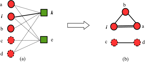
Figure 2: Mode-1 nodes are circles and mode-2 nodes are squares, while dashed and continuous outlines indicate different levels of a mode-1 nodal attribute. In (a), edge $i\longleftrightarrow k$ is part of two distinct two-paths joining matching mode-1 nodes, $a$—$k$—$i$ and $b$—$k$—$i$. In (b), we see the projection of (a) onto mode-1 nodes, with multiplicity indicated as appropriate.

By contrast, a different reformulation of Equation (3) gives

$$\mbox{b1nodematch}(\mathchoice{\mbox{$\mathbf{\displaystyle}\bf y$}}{\mbox{$\mathbf{\textstyle}\bf y$}}{\mbox{$\mathbf{\scriptstyle}\bf y$}}{\mbox{$\mathbf{\scriptscriptstyle}\bf y$}})=\frac{1}{2}\sum_{i=1}^{n_{1}}\sum_{\stackrel{{\scriptstyle j\neq i:}}{{\mbox{\scriptsize$c_{j}=c_{i}$}}}}\left[\sum_{k=n_{1}+1}^{n_{1}+n_{2}}y_{ik}y_{kj}\right],$$ (5)

where the sum is taken over all pairs $i\neq j$ of matching mode 1 nodes; in this double sum, $(i,j)$ and $(j,i)$ are counted as distinct node pairs, so again we divide by two to correct for the double-counting. We refer to Equation (5) as the node-centered view, because it counts, in the square brackets, the number of two-paths that connect each pair $\{i,j\}$ of matching nodes. Using the network in Figure 2(b), this count of two-paths equals 2 if $j=a$ and 1 if $j=b$.

Our modification to the two-star count involves modifying either Equation (4) or Equation (5) by including an exponent in the range $[0,1]$. In the node-centered view (5), we use the exponent $\alpha$, which results in

$$\mbox{b1nodematch}(\mathchoice{\mbox{$\mathbf{\displaystyle}\bf y$}}{\mbox{$\mathbf{\textstyle}\bf y$}}{\mbox{$\mathbf{\scriptstyle}\bf y$}}{\mbox{$\mathbf{\scriptscriptstyle}\bf y$}};\alpha)=\frac{1}{2}\sum_{i=1}^{n_{1}}\sum_{\stackrel{{\scriptstyle j\neq i:}}{{\mbox{\scriptsize$c_{j}=c_{i}$}}}}\left[\sum_{k=n_{1}+1}^{n_{1}+n_{2}}y_{ik}y_{kj}\right]^{\alpha}\quad\mbox{with $0\leq\alpha\leq 1$}.$$ (6)

On the other hand, if we take the edge-centered view (4), we use the exponent $\beta$, which gives

$$\mbox{b1nodematch}(\mathchoice{\mbox{$\mathbf{\displaystyle}\bf y$}}{\mbox{$\mathbf{\textstyle}\bf y$}}{\mbox{$\mathbf{\scriptstyle}\bf y$}}{\mbox{$\mathbf{\scriptscriptstyle}\bf y$}};\beta)=\frac{1}{2}\sum_{i=1}^{n_{1}}\sum_{k=n_{1}+1}^{n_{1}+n_{2}}y_{ik}\left[\mathop{\sum}_{\stackrel{{\scriptstyle j\neq i:}}{{\mbox{\scriptsize$c_{j}=c_{i}$}}}}y_{jk}\right]^{\beta}\quad\mbox{with $0\leq\beta\leq 1$}.$$ (7)

When $\alpha=0$ or $\beta=0$ in Equations (6) and (7), we interpret the expression $0^{0}$ as zero, since the base will always be an integer whereas the exponent can take values in $[0,1]$; thus, $0^{0}$ is most sensibly interpreted as $\lim_{\epsilon\to 0}0^{\epsilon}=0$.

Equations (6) and (7) may be modified slightly if we wish to consider only nodes matching a certain value $v$. This modification yields the terms

$$\mbox{b1nodematch}_{v}(\mathchoice{\mbox{$\mathbf{\displaystyle}\bf y$}}{\mbox{$\mathbf{\textstyle}\bf y$}}{\mbox{$\mathbf{\scriptstyle}\bf y$}}{\mbox{$\mathbf{\scriptscriptstyle}\bf y$}};\alpha)=\frac{1}{2}\sum_{i=1}^{n_{1}}\mathop{\sum}_{\stackrel{{\scriptstyle j\neq i:}}{{\mbox{\scriptsize$c_{j}=c_{i}=v$}}}}\left[\sum_{k=n_{1}+1}^{n_{1}+n_{2}}y_{ik}y_{kj}\right]^{\alpha}$$ (8)

and

$$\mbox{b1nodematch}_{v}(\mathchoice{\mbox{$\mathbf{\displaystyle}\bf y$}}{\mbox{$\mathbf{\textstyle}\bf y$}}{\mbox{$\mathbf{\scriptstyle}\bf y$}}{\mbox{$\mathbf{\scriptscriptstyle}\bf y$}};\beta)=\frac{1}{2}\sum_{i=1}^{n_{1}}\sum_{k=n_{1}+1}^{n_{1}+n_{2}}y_{ik}\left[\mathop{\sum}_{\stackrel{{\scriptstyle j\neq i:}}{{\mbox{\scriptsize$c_{j}=c_{i}=v$}}}}y_{jk}\right]^{\beta}.$$ (9)

The versions of the statistics in Equations (6) and (7) model what is called “uniform” homophily, since the homophily effect is implicitly presumed to be the same for all levels of the categorical variable. By contrast, Equations (8) and (9) model “differential” homophily in which each level $v$ of the categorical variable corresponds to a separate statistic, and not all levels’ statistics need be included in the ERGM.

3.2 Theoretical considerations

When $\alpha=\beta=1$, the two statistics of Equations (6) and (7) are equal to one another and to the full count of two-stars with matching endpoints. On the other end of the spectrum, when $\alpha=0$, statistic (6) counts the number of matching node pairs connected by at least one two-path. When $\beta=0$, statistic (7) counts the number of edges involved in at least one matching two-star. The case $\alpha=0$ is the only case other than $\alpha=\beta=1$ where we know of an analogue elsewhere in the literature: If the alternating $k$-twopath statistic of Wang et al. (2009, Equation 6.13) is extended to a matching-attribute-based alternating $k$-twopath statistic, then statistic (6) with $\alpha=0$ is equivalent to its special case of $\lambda_{t}=1$. However, we are not aware of any other direct correspondences between existing ERGM statistics and either of Equations (6) or  (7).

The network statistics we have introduced are curved exponential family model terms in the sense of Hunter and Handcock (2006), which is a mathematically useful feature explained in Appendix B. In practical terms, this means that it should be possible to model $\mathbf{\textstyle}\bf\theta$ and the discount parameter jointly, rather than taking the profile likelihood approach that we have done here where the likelihood is maximized only with respect to $\mathbf{\textstyle}\bf\theta$ for fixed $\alpha$ or $\beta$ on a grid of values in $[0,1]$. However, as of the writing of this manuscript, the ergm package implementation of the b1nodematch and b2nodematch model terms does not exploit ergm’s full curved parameter capabilities.

Finally, models with the b1nodematch or b2nodematch terms can exhibit a mathematically unusual property. Consider Model (1) with $p=1$ and $s_{1}(\mathchoice{\mbox{$\mathbf{\displaystyle}\bf y$}}{\mbox{$\mathbf{\textstyle}\bf y$}}{\mbox{$\mathbf{\scriptstyle}\bf y$}}{\mbox{$\mathbf{\scriptscriptstyle}\bf y$}})=\mbox{b1nodematch}(\mathchoice{\mbox{$\mathbf{\displaystyle}\bf y$}}{\mbox{$\mathbf{\textstyle}\bf y$}}{\mbox{$\mathbf{\scriptstyle}\bf y$}}{\mbox{$\mathbf{\scriptscriptstyle}\bf y$}};\alpha)$; that is,

$$P(\mathchoice{\mbox{$\mathbf{\displaystyle}\bf Y$}}{\mbox{$\mathbf{\textstyle}\bf Y$}}{\mbox{$\mathbf{\scriptstyle}\bf Y$}}{\mbox{$\mathbf{\scriptscriptstyle}\bf Y$}}=\mathchoice{\mbox{$\mathbf{\displaystyle}\bf y$}}{\mbox{$\mathbf{\textstyle}\bf y$}}{\mbox{$\mathbf{\scriptstyle}\bf y$}}{\mbox{$\mathbf{\scriptscriptstyle}\bf y$}})=\frac{\exp\{\theta\times\mbox{b1nodematch}(\mathchoice{\mbox{$\mathbf{\displaystyle}\bf y$}}{\mbox{$\mathbf{\textstyle}\bf y$}}{\mbox{$\mathbf{\scriptstyle}\bf y$}}{\mbox{$\mathbf{\scriptscriptstyle}\bf y$}};\alpha)\}}{\kappa(\mathchoice{\mbox{$\mathbf{\displaystyle}\bf\theta$}}{\mbox{$\mathbf{\textstyle}\bf\theta$}}{\mbox{$\mathbf{\scriptstyle}\bf\theta$}}{\mbox{$\mathbf{\scriptscriptstyle}\bf\theta$}})}$$ (10)

for specific values $\theta$ and $\alpha$. Then this ERGM is a dyadic dependence model in the sense that the individual dyads—that is, the Bernoulli random variables $Y_{ik}$—are not mutually independent. Let $V=V_{1}\cup V_{2}$ denote the set of vertices, or nodes, decomposed into the mode 1 vertices $V_{1}$ and the mode 2 vertices $V_{2}$. For nonempty subsets $W_{1}\subset V_{1}$ and $W_{2}\subset V_{2}$, consider the possible bipartite networks on the nodes $W=W_{1}\cup W_{2}$, where only edges connecting a node in $W_{1}$ with a node in $W_{2}$ are permitted. According to a result of Shalizi and Rinaldo (2013), Model (10) is not projective, which means that if we marginalize over all networks on $V$ to get the marginal distribution for networks on $W$, this distribution is not the same as Equation (10) for the set of networks on $W$ for all possible choices of $W_{1}$ and $W_{2}$. However, Model (10) does enjoy a limited projectivity property: Projectivity holds for the set of networks on any $W$ of the form $V_{1}\cup W_{2}$, where $W_{2}\subset V_{2}$. This property means, for instance, that standard properties such as consistency and asymptotic normality of maximum likelihood estimators hold if we fix $n_{1}$ and let $n_{2}$ tend to $\infty$. These results hold if $\beta$ replaces $\alpha$ in Equation (10) or if additional dyadic independence statistics are added to the $\mathchoice{\mbox{$\mathbf{\displaystyle}\bf s$}}{\mbox{$\mathbf{\textstyle}\bf s$}}{\mbox{$\mathbf{\scriptstyle}\bf s$}}{\mbox{$\mathbf{\scriptscriptstyle}\bf s$}}(\mathchoice{\mbox{$\mathbf{\displaystyle}\bf y$}}{\mbox{$\mathbf{\textstyle}\bf y$}}{\mbox{$\mathbf{\scriptstyle}\bf y$}}{\mbox{$\mathbf{\scriptscriptstyle}\bf y$}})$ vector.

3.3 Interpreting Model Coefficients

As a means for understanding the homophily statistics introduced in the previous section, we first describe the notion of change statistics that is central to the theory of ERGMs. Given a network $\mathchoice{\mbox{$\mathbf{\displaystyle}\bf y$}}{\mbox{$\mathbf{\textstyle}\bf y$}}{\mbox{$\mathbf{\scriptstyle}\bf y$}}{\mbox{$\mathbf{\scriptscriptstyle}\bf y$}}\in{\cal Y}$, the vector $\mathchoice{\mbox{$\mathbf{\displaystyle}\bf s$}}{\mbox{$\mathbf{\textstyle}\bf s$}}{\mbox{$\mathbf{\scriptstyle}\bf s$}}{\mbox{$\mathbf{\scriptscriptstyle}\bf s$}}(\mathchoice{\mbox{$\mathbf{\displaystyle}\bf y$}}{\mbox{$\mathbf{\textstyle}\bf y$}}{\mbox{$\mathbf{\scriptstyle}\bf y$}}{\mbox{$\mathbf{\scriptscriptstyle}\bf y$}})=s_{1}(\mathchoice{\mbox{$\mathbf{\displaystyle}\bf y$}}{\mbox{$\mathbf{\textstyle}\bf y$}}{\mbox{$\mathbf{\scriptstyle}\bf y$}}{\mbox{$\mathbf{\scriptscriptstyle}\bf y$}}),\ldots,s_{p}(\mathchoice{\mbox{$\mathbf{\displaystyle}\bf y$}}{\mbox{$\mathbf{\textstyle}\bf y$}}{\mbox{$\mathbf{\scriptstyle}\bf y$}}{\mbox{$\mathbf{\scriptscriptstyle}\bf y$}})$ of statistics from the ERGM of Equation (1) yields a set of change statistics that may be viewed as the off-diagonal entries of an $n\times n$ matrix whose $(i,j)$ entry is defined as

$$\mathchoice{\mbox{$\mathbf{\displaystyle}\bf\delta$}}{\mbox{$\mathbf{\textstyle}\bf\delta$}}{\mbox{$\mathbf{\scriptstyle}\bf\delta$}}{\mbox{$\mathbf{\scriptscriptstyle}\bf\delta$}}_{\mathchoice{\mbox{$\mathbf{\displaystyle}\bf s$}}{\mbox{$\mathbf{\textstyle}\bf s$}}{\mbox{$\mathbf{\scriptstyle}\bf s$}}{\mbox{$\mathbf{\scriptscriptstyle}\bf s$}}}(\mathchoice{\mbox{$\mathbf{\displaystyle}\bf y$}}{\mbox{$\mathbf{\textstyle}\bf y$}}{\mbox{$\mathbf{\scriptstyle}\bf y$}}{\mbox{$\mathbf{\scriptscriptstyle}\bf y$}})_{ij}=\mathchoice{\mbox{$\mathbf{\displaystyle}\bf s$}}{\mbox{$\mathbf{\textstyle}\bf s$}}{\mbox{$\mathbf{\scriptstyle}\bf s$}}{\mbox{$\mathbf{\scriptscriptstyle}\bf s$}}(\mathchoice{\mbox{$\mathbf{\displaystyle}\bf y$}}{\mbox{$\mathbf{\textstyle}\bf y$}}{\mbox{$\mathbf{\scriptstyle}\bf y$}}{\mbox{$\mathbf{\scriptscriptstyle}\bf y$}}_{ij}^{+})-\mathchoice{\mbox{$\mathbf{\displaystyle}\bf s$}}{\mbox{$\mathbf{\textstyle}\bf s$}}{\mbox{$\mathbf{\scriptstyle}\bf s$}}{\mbox{$\mathbf{\scriptscriptstyle}\bf s$}}(\mathchoice{\mbox{$\mathbf{\displaystyle}\bf y$}}{\mbox{$\mathbf{\textstyle}\bf y$}}{\mbox{$\mathbf{\scriptstyle}\bf y$}}{\mbox{$\mathbf{\scriptscriptstyle}\bf y$}}_{ij}^{-}),$$

where $\mathchoice{\mbox{$\mathbf{\displaystyle}\bf y$}}{\mbox{$\mathbf{\textstyle}\bf y$}}{\mbox{$\mathbf{\scriptstyle}\bf y$}}{\mbox{$\mathbf{\scriptscriptstyle}\bf y$}}_{ij}^{+}$ and $\mathchoice{\mbox{$\mathbf{\displaystyle}\bf y$}}{\mbox{$\mathbf{\textstyle}\bf y$}}{\mbox{$\mathbf{\scriptstyle}\bf y$}}{\mbox{$\mathbf{\scriptscriptstyle}\bf y$}}_{ij}^{-}$ represent the networks obtained by fixing $y_{ij}=1$ or $y_{ij}=0$, respectively, and keeping all other entries the same as in $\mathbf{\textstyle}\bf y$ itself. These change statistics are important because under the ERGM of Equation (1), the conditional log-odds that $Y_{ij}=1$, conditional on all other entries in $\mathbf{\textstyle}\bf Y$ (denoted by $\mathchoice{\mbox{$\mathbf{\displaystyle}\bf Y$}}{\mbox{$\mathbf{\textstyle}\bf Y$}}{\mbox{$\mathbf{\scriptstyle}\bf Y$}}{\mbox{$\mathbf{\scriptscriptstyle}\bf Y$}}_{ij}^{c}$), may be expressed as

$$\log\frac{P_{\mathchoice{\mbox{$\mathbf{\displaystyle}\bf\theta$}}{\mbox{$\mathbf{\textstyle}\bf\theta$}}{\mbox{$\mathbf{\scriptstyle}\bf\theta$}}{\mbox{$\mathbf{\scriptscriptstyle}\bf\theta$}}}(Y_{ij}=1\mid\mathchoice{\mbox{$\mathbf{\displaystyle}\bf Y$}}{\mbox{$\mathbf{\textstyle}\bf Y$}}{\mbox{$\mathbf{\scriptstyle}\bf Y$}}{\mbox{$\mathbf{\scriptscriptstyle}\bf Y$}}_{ij}^{c}=\mathchoice{\mbox{$\mathbf{\displaystyle}\bf y$}}{\mbox{$\mathbf{\textstyle}\bf y$}}{\mbox{$\mathbf{\scriptstyle}\bf y$}}{\mbox{$\mathbf{\scriptscriptstyle}\bf y$}}_{ij}^{c})}{P_{\mathchoice{\mbox{$\mathbf{\displaystyle}\bf\theta$}}{\mbox{$\mathbf{\textstyle}\bf\theta$}}{\mbox{$\mathbf{\scriptstyle}\bf\theta$}}{\mbox{$\mathbf{\scriptscriptstyle}\bf\theta$}}}(Y_{ij}=0\mid\mathchoice{\mbox{$\mathbf{\displaystyle}\bf Y$}}{\mbox{$\mathbf{\textstyle}\bf Y$}}{\mbox{$\mathbf{\scriptstyle}\bf Y$}}{\mbox{$\mathbf{\scriptscriptstyle}\bf Y$}}_{ij}^{c}=\mathchoice{\mbox{$\mathbf{\displaystyle}\bf y$}}{\mbox{$\mathbf{\textstyle}\bf y$}}{\mbox{$\mathbf{\scriptstyle}\bf y$}}{\mbox{$\mathbf{\scriptscriptstyle}\bf y$}}_{ij}^{c})}=\mathchoice{\mbox{$\mathbf{\displaystyle}\bf\theta$}}{\mbox{$\mathbf{\textstyle}\bf\theta$}}{\mbox{$\mathbf{\scriptstyle}\bf\theta$}}{\mbox{$\mathbf{\scriptscriptstyle}\bf\theta$}}^{\top}\mathchoice{\mbox{$\mathbf{\displaystyle}\bf\delta$}}{\mbox{$\mathbf{\textstyle}\bf\delta$}}{\mbox{$\mathbf{\scriptstyle}\bf\delta$}}{\mbox{$\mathbf{\scriptscriptstyle}\bf\delta$}}_{\mathchoice{\mbox{$\mathbf{\displaystyle}\bf s$}}{\mbox{$\mathbf{\textstyle}\bf s$}}{\mbox{$\mathbf{\scriptstyle}\bf s$}}{\mbox{$\mathbf{\scriptscriptstyle}\bf s$}}}(\mathchoice{\mbox{$\mathbf{\displaystyle}\bf y$}}{\mbox{$\mathbf{\textstyle}\bf y$}}{\mbox{$\mathbf{\scriptstyle}\bf y$}}{\mbox{$\mathbf{\scriptscriptstyle}\bf y$}})_{ij}.$$ (11)

Equation (11) arises directly from Equation (1) via simple algebra and omits the troublesome factor $\kappa(\mathchoice{\mbox{$\mathbf{\displaystyle}\bf\theta$}}{\mbox{$\mathbf{\textstyle}\bf\theta$}}{\mbox{$\mathbf{\scriptstyle}\bf\theta$}}{\mbox{$\mathbf{\scriptscriptstyle}\bf\theta$}})$, a fact that is useful in myriad ways such as simulating random networks whose distribution is approximately $P_{\mathchoice{\mbox{$\mathbf{\displaystyle}\bf\theta$}}{\mbox{$\mathbf{\textstyle}\bf\theta$}}{\mbox{$\mathbf{\scriptstyle}\bf\theta$}}{\mbox{$\mathbf{\scriptscriptstyle}\bf\theta$}}}(\cdot)$ via MCMC (Hunter et al., 2008, Section 6).

Equation (11) also reveals that, for $1\leq\ell\leq p$, the $\ell$th element $\theta_{\ell}(\mathchoice{\mbox{$\mathbf{\displaystyle}\bf\delta$}}{\mbox{$\mathbf{\textstyle}\bf\delta$}}{\mbox{$\mathbf{\scriptstyle}\bf\delta$}}{\mbox{$\mathbf{\scriptscriptstyle}\bf\delta$}}_{\mathchoice{\mbox{$\mathbf{\displaystyle}\bf s$}}{\mbox{$\mathbf{\textstyle}\bf s$}}{\mbox{$\mathbf{\scriptstyle}\bf s$}}{\mbox{$\mathbf{\scriptscriptstyle}\bf s$}}}(\mathchoice{\mbox{$\mathbf{\displaystyle}\bf y$}}{\mbox{$\mathbf{\textstyle}\bf y$}}{\mbox{$\mathbf{\scriptstyle}\bf y$}}{\mbox{$\mathbf{\scriptscriptstyle}\bf y$}})_{ij})_{\ell}$ is the change in the log-odds of the entire network resulting from changing the $i,j$ edge from 0 to 1, holding everything else equal. For instance, in Equation (2), we see that $(\mathchoice{\mbox{$\mathbf{\displaystyle}\bf\delta$}}{\mbox{$\mathbf{\textstyle}\bf\delta$}}{\mbox{$\mathbf{\scriptstyle}\bf\delta$}}{\mbox{$\mathbf{\scriptscriptstyle}\bf\delta$}}_{\mathchoice{\mbox{$\mathbf{\displaystyle}\bf s$}}{\mbox{$\mathbf{\textstyle}\bf s$}}{\mbox{$\mathbf{\scriptstyle}\bf s$}}{\mbox{$\mathbf{\scriptscriptstyle}\bf s$}}}(\mathchoice{\mbox{$\mathbf{\displaystyle}\bf y$}}{\mbox{$\mathbf{\textstyle}\bf y$}}{\mbox{$\mathbf{\scriptstyle}\bf y$}}{\mbox{$\mathbf{\scriptscriptstyle}\bf y$}})_{ij})_{1}=1$ and $(\mathchoice{\mbox{$\mathbf{\displaystyle}\bf\delta$}}{\mbox{$\mathbf{\textstyle}\bf\delta$}}{\mbox{$\mathbf{\scriptstyle}\bf\delta$}}{\mbox{$\mathbf{\scriptscriptstyle}\bf\delta$}}_{\mathchoice{\mbox{$\mathbf{\displaystyle}\bf s$}}{\mbox{$\mathbf{\textstyle}\bf s$}}{\mbox{$\mathbf{\scriptstyle}\bf s$}}{\mbox{$\mathbf{\scriptscriptstyle}\bf s$}}}(\mathchoice{\mbox{$\mathbf{\displaystyle}\bf y$}}{\mbox{$\mathbf{\textstyle}\bf y$}}{\mbox{$\mathbf{\scriptstyle}\bf y$}}{\mbox{$\mathbf{\scriptscriptstyle}\bf y$}})_{ij})_{2}=I\{\mbox{$i$ and $j$ are of the same gender}\}$ for all $i<j$, and these values do not depend on any of the values in $\mathchoice{\mbox{$\mathbf{\displaystyle}\bf y$}}{\mbox{$\mathbf{\textstyle}\bf y$}}{\mbox{$\mathbf{\scriptstyle}\bf y$}}{\mbox{$\mathbf{\scriptscriptstyle}\bf y$}}_{ij}^{c}$. Therefore, adding (subtracting) the edge $(i,j)$ increases (decreases) the log-odds of the entire network by either $\theta_{1}$ or $\theta_{1}+\theta_{2}$, depending on whether $i$ and $j$ are of the same gender, independent of the rest of the network. In Section 4, we similarly interpret fitted models involving the homophily terms introduced here.

4 Substantive Findings in Two-Mode Network Datasets

In this section, we demonstrate that the proposed bipartite homophily statistics give rise to meaningful results that allow for a more substantial integration with theoretical considerations proposed by social scientists than the basic statistic of Equation (3). We do so by applying them to the two datasets introduced in the introduction: A network in which employees of an organization are affiliated with their core competencies and a network of directors that are affiliated with different firms. We contrast two approaches to using the reformulated homophily effects: First, a profile likelihood approach, which allows researchers to take a more explorative perspective that is relatively agnostic to prior theory, and second, a theory-based approach, that is relatively agnostic to changes in the log-likelihood.

4.1 Competence network

For the competence network discussed in Section 1, $n_{1}=176$ actors were asked to list up to three core competencies each from a list of $n_{2}=33$ competencies. Competencies included a variety of topics, such as financial analysis, information technology, marketing in the context of different countries, and industrial sales. Social scientists researching such a network may be interested in the role of hard skill competencies which refer to concrete abilities such as having knowledge about a manufacturing process and are nested in the individual, versus competencies that are more integrated into the organizational structure, such as the capability for strategic planning or privileges for commodities procurement. Understanding the distribution of competencies and skills across an organization—for example, if employees who list hard skills typically do not list softer skills as their core competencies—may help to provide insights into how businesses perform (Chin and Md Yusoff, 2020), how effective projects are managed (de Carvalho and Junior, 2015), or how organizational or educational training programs are conceived (Robles, 2012; Laker and Powell, 2011). In our analysis, we are thus interested in exploring if hard and softer skills are listed in homophilic patterns. To that end, we coded each competency as either “hard skills” or “not hard skills” and use the term b2nodematch("hardskill", [formulation] = [value]), where [formulation] may be replaced by alpha for the node-centric formulation or beta for the edge-centric formulation and [value] may be replaced by a value from 0 to 1. The b2nodematch parameter estimated here works analogously to the b1nodematch equations presented in Section 3, but centers on the “events” mode—in this case, competencies. In addition, we include the edges term, which controls the overall density of the network and is useful in much the same way that it is typically useful to include an intercept term in any logistic regression model. In addition, we control for the effect of tenure of the employees, via b1cov("tenure"), and the effect of gender, via b1factor("gender").

We approached the selection of $\alpha$ or $\beta$ values using a profile likelihood approach, thus fitting separate models for each parameter over a grid of points from 0 to 1. All models converged without issues. As is evident from the visualization in Figure 3(a), the estimated profile likelihood suggests an optimal value of alpha=0. This means that homophily is measured by how many pairs of competences with the same categorization (hard vs. not) are found in at least one employee; absent a substantive reason to prefer a particular homophily statistic, this version might be considered the best choice based on its profile likelihood. Table 1 presents the estimated parameters for the $\alpha=0$ model.

Figure 3: Left to right are (a) the approximate maximum log-likelihood values, (b) the coefficient estimates for the hardskill homophily term, and (c) the p-values associated with the hypothesis tests that the coefficients are zero, respectively, as a function of $\alpha$ (the A’s) and $\beta$ (the B’s).

Table 1: Parameter estimates and standard errors for the competency dataset, along with ergm code used to obtain them. Statistical significance at the 0.05, 0.001, and 0.0001 level is indicated by *, **, and ***, respectively.

	Statistic	Parameter estimate (S.E.)
	edges	$-1.936$ (0.152)***
	b1cov.tenure	$-0.001$ (0.047)***
	b1factor.gender.Male	$0.069$ (0.120)***
	b2nodematch.hardskill	$-1.121$ (0.123)***
Code in ergm:
ergm(formula = net_tm $\sim$ edges + b1cov("tenure") +
b1factor("gender") + b2nodematch("hardskill", alpha = 0),
control = control.ergm(MCMC.samplesize = 15000, seed = 123456))

Our model leads to an estimated negative homophily effect: It is less likely that two competencies sharing the same soft/hard designation will be listed by the same employee than would be predicted by chance, after accounting for the observed overall density and the differential numbers of competencies listed by people of different genders and tenures. This effect persists when alternative model terms are considered. For instance, we tried correcting for each individual competency’s tendency to be named by employees, which is accomplished by adding the b2sociality model term. In this case, the model with the highest estimated log-likelihood was the $\alpha=0.5$ model, corresponding to a statistic in which homophily is measured by summing, for each pair of matching competencies, the square root of the number of employees who named both. In this model and all of the models containing b2sociality, the homophily effect was statistically significantly negative. We also duplicated the model terms shown in Table 1 but using the diff = TRUE option with the b2nodematch term. This modification implements differential homophily, replacing the single statistic in Equation (6) by two statistics of the form (8), one for $v=0$ (soft skills) and one for $v=1$ (hard skills). The results revealed no interesting qualitative difference in the two homophily effects nor any deviation from the overall results shown in Figure 3.

In this case, we explored the full range of homophily parameters and described the social implications post-hoc. Social scientists might prefer to let theory and hypothesis drive the construction of statistical models. We give an example for such an approach in our next illustration.

4.2 Fortune 500 directorates

The role of gender in corporate governance and social elite cohesion is the subject of long-standing yet contemporary debates (Sidhu et al., 2021; Sojo et al., 2016; Kesner, 1988). Management scholars and sociologists alike have examined the formation and outcomes of gender diversity on corporate boards. For instance, Seebeck and Vetter (2021) find that gender diversity on boards is positively related to the disclosure of corporate risks. Kim and Starks (2016) find that diversified corporate boards improve firm value through additional expertise and unique skills. Other studies find that overall corporate performance tends to improve as a consequence of gender diversity on boards (O’Hagan, 2017; Erhardt, Werbel and Shrader, 2003), solidifying the emerging consensus that females ascending “through the ceilings of upper-middle management into strategy-making roles in the highest echelons, has a net benefit for firms in the long run” (Jeong and Harrison, 2017). Given these net benefits, it is perhaps surprising that, even today, data “unequivocally show that around the world, men hold the vast majority of corporate directorships and women are starkly underrepresented” (Kirsch, 2018).

Here, we propose that, in addition to the well-known proverbial glass ceiling that prevents women from rising further in the ranks of a company after achieving a certain threshold in their career, there is also a glass door. This effect is in evidence after women have already obtained leadership positions, such as serving on a firm’s board of directors, serving to ease further integration by women onto these boards. Analyzing this horizontal integration contributes to research on the role of gender in board compositions and allows for novel insights into the phenomenon of social elite cohesion (Davis, Yoo and Baker, 2003; Park and Westphal, 2013). We will now demonstrate that the reformulated nodematch effects we propose in this paper allow for a nuanced analysis of the role of gender homophily, which helps to explain how women already present on boards may help to mitigate the effect of a proverbial glass door.

To that end, we take an edge-centric view of homophily. That is, given a particular edge between a female and a particular board, how likely is it that other females serve on the same board? This is opposed to the node-centered view, which simply asks whether a given pair of females is more or less likely to sit on a board together than pure chance might predict. These two views coincide when $\alpha=\beta=1$, but for values of $\alpha$ or $\beta$ strictly less than 1, the use of $\beta$ seems more appropriate for this application. Furthermore, the test for the glass door effect suggests a low value of $\beta$; in the extreme when $\beta=0$, the nodematch term is the count, over all female-board combinations, of how many have at least one additional female on the same board. The value $\beta=(\alpha=)1$, on the other hand, suggests that this glass door is opened much more widely as the number of women increases, with the effect increasing quadratically in the number of women. We argue that such a measure of homophily is inappropriate here; instead, our hypothesis is that the first women serving on the board of a given firm somewhat normalize the idea of female directors serving on the boards of said firms; after a few female directors, however, this effect decreases, as the notion of female directors serving the firm in an equal capacity has already been established. In other words, based on wholly substantive considerations, we believe that homophily in this case is captured most appropriately by a $\beta$ value that is small but strictly positive.

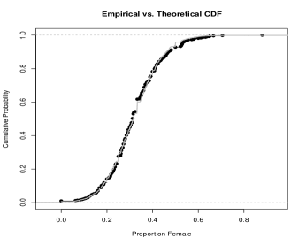
Figure 4: Comparison of empirical (black dots) with theoretical (gray lines) cumulative distribution functions under the assumption of no gender-based homophily for female proportions on 489 boards of directors.

To estimate the gender homophily effect in practice, we analyze a network of directorate memberships among Fortune 500 companies in 2022. Our sample consists of $n_{1}=489$ firms and $n_{2}=8606$ directors. Here, directors are affiliated with different firms, constituting a two-mode structure. Preliminary exploration suggests that if a nonzero gender homophily effect exists, it might be subtle. Figure 4 depicts the empirical cumulative distribution of the 489 values of $\hat{p}_{F}$, the sample proportion of females, among all of the boards. If gender is irrelevant in board composition, we might expect that this distribution roughly mimics what would occur if every board’s gender makeup were binomially distributed with parameters equal to the observed size of the board and the overall fraction, $2741/8606$, of females among all directors. As shown in Figure 4, these two distribution functions are quite close.

Additional exploratory analysis of the Fortune 500 dataset provides another reason to prefer a $\beta$-based measure of homophily rather than an $\alpha$-based measure, once we rule out the $\alpha=1$ idea for substantive reasons: In this dataset, nearly all pairs of females who serve on any board together serve on exactly one board together. This fact is revealed if we compare the value of the nodematch(alpha = 0) statistic, $10{,}582$, to the nodematch(alpha = 1) statistic, $10{,}592$. In other words, the $\alpha$-based homophily effects for this dataset are essentially all equivalent. In contrast, the female nodematch(beta = 0) statistic equals only 1562, suggesting that this dataset has nuanced information regarding the propensity for females serving on a board to predict whether other females also serve on that board and validating our decision to focus on a low $\beta$ value to address our substantive question about gender homophily on boards of directors. Interestingly, a profile likelihood approach does not suggest a clear model choice in this case, as shown in Figure 5(a).

Figure 5(a) shows the different parameter estimates produced by different $\alpha$ and $\beta$ values from 0 to 1. All estimates are significant at $p<0.001$ except the $\beta=0$ case, which was also considerably more difficult than others for ergm’s MCMC-based estimation procedure to fit. Indeed, the fitting procedure hinted at near-collinearity in the $\beta=0$ case, providing another reason to select a strictly positive $\beta$ value.

Figure 5: Shown as a function of $\alpha$ (the A’s) and $\beta$ (the B’s) are (a) at left, the MCMC- based maximum log-likelihood approximations, each with an estimated standard deviation of 1; and (b) at right, the coefficient estimates for the female homophily term.

Estimated coefficients for a model using $\beta=0.1$ that also corrects for nodal covariates including gender (for directors) and assets and industry sector (for companies) are shown in Table 2. This model also corrects for the overall propensity for directors to join multiple boards, via b2star(2) and b2degree(1), without regard to gender. The ability to correct for such effects, in a regression-like setting, for nodes from each of the two modes is one of the virtues of the methods presented here that retain the full bipartite structure of the dataset.

Differentiating between the effects of gender homophily for men and women shows that the estimated effect is stronger for women than for their male counterparts. However, this difference is not statistically significant; in the fitted model summarized by Table 2, the difference between the female and male homophily coefficient estimates equals $0.85$ whereas the estimated standard error of this difference is $0.94$. Such contrasts may be analyzed using standard techniques because the fitted model produced by the ergm package includes an estimated covariance matrix.

Table 2: Parameter estimates and standard errors for the directorates dataset, using $\beta=0.1$ for the homophily terms, along with ergm code used to obtain them. Statistical significance at the 0.0001 level is indicated by ***.

	Statistic	Parameter estimate (S.E.)
	edges	$-7.61$ (0.59)***
	b2star2	$-2.47$ (0.17)***
	b2degree(1)	$3.48$ (0.17)***
	b1cov.log10_total_assets	$0.097$ (0.018)***
	b1factor.industry_sector.2	$-0.030$ (0.035)***
	b1factor.industry_sector.3	$0.039$ (0.053)***
	b1factor.industry_sector.4	$0.097$ (0.051)***
	b1factor.industry_sector.5	$-0.086$ (0.034)***
	b1factor.industry_sector.6	$0.030$ (0.046)***
	b2nodematch.gender.Female	$3.75$ (0.67)***
	b2nodematch.gender.Male	$2.90$ (0.72)***
	b2factor.gender.Male	$0.12$ (0.66)***
	b2cov.age	$0.045$ (0.004)***
Code in ergm:
ergm(Directorships $\sim$ edges + b2star(2) + b2degree(1)
+ b1cov("log10_total_assets") + b1factor("industry_sector")
+ b2nodematch("gender", beta = 0.1, diff = TRUE)
+ b2factor("gender") + b2cov("age")

Our findings contribute to ongoing discussions about women in the boardroom (Kirsch, 2018; Mah et al., 2022), illuminating how a different perspective on homophily that takes bipartite structures into account leads to novel approaches to long-standing questions.

5 Discussion

Apart from the statistical benefits, such as increased modeling flexibility and improved model fit, the reformulated nodematch effects presented here offer exciting avenues for future research for scholars interested in social network analysis. Most notably, the reformulated effects enable questions that do not simply employ a one-mode perspective on homophily after projecting from a two-mode network. Rather, they are built with the properties of two-mode networks in mind, allowing for the differentiation of two fundamentally different theoretical constructs: Homophily based on enumerating paths that connect a particular node pair with the same attributes, versus homophily based on counting completed two-paths with matching end nodes that include a particular tie. Only in the case where these counts contribute linearly to the corresponding homophily statistics are these two views equivalent.

We present two real-world applications to demonstrate both of these perspectives and find contrasting results: For the first network, in which employees are connected through shared competences they were asked to list, the node-centric view dramatically alters the estimated models’ statistical properties and therefore the substantive conclusions we derive from analyzing the observed network. For the second network, which depicts board memberships among Fortune 500 companies, the edge-centric reformulation provides insight into pressing questions that so far had remained unanswered. These two contrasting results underscore that the reformulated effects we present in this article allow for theory-building and subsequent empirical testing from a novel yet natural two-mode perspective.

The methods illustrated here are available in the ergm package for R, where they may be used in conjunction with a wide range of other statistics. The specific statistics included in an ERGM will depend on the modeling aims particular to the situation and, as always, the interpretation of coefficients from a fitted model must be done in the presence of all other model terms. General treatments of ERGMs (e.g., Robins et al., 2007a) or articles specific to the bipartite network setting (e.g., Wang et al., 2009, 2013) provide insight into additional model terms that may be of interest.

6 Acknowledgments

This work is supported by NIH grant R01-GM083603-01. The authors are grateful to Shweta Bansal of Georgetown University, who was involved in early conversations about this manuscript and who supplied motivating examples not actually used here. The data on competencies were graciously provided by Andrew Parker of Durham University.

Appendix A Change Statistics

In addition to providing insight on model coefficients as explained in Section 3.3, examination of change statistics may sometimes identify possible degeneracy problems with an ERGM: If a change statistic can grow exceedingly large in the positive or negative direction, then a corresponding $\theta$ coefficient of the same or opposite sign can virtually assure the presence or absence of an edge, and this type of behavior can become self-reinforcing. We do not delve into details of the degeneracy issue here, referring interested readers instead to Handcock (2003) and Schweinberger (2011).

This section presents change statistics for both the node-centered ($\alpha$-based) and edge-centered ($\beta$-based) homophily statistics introduced in this article. First, fix a node pair $(i,k)$, where $i$ belongs to mode 1, $k$ belongs to mode 2, and $c$ is a categorical nodal attribute measured on the mode 1 nodes. We will focus on the b1nodematch change statistics, though the arguments below may easily be adapted to the b2nodematch case.

The corresponding change statistics are obtained by calculating the difference between the contributions to the statistic with $y_{ik}=1$ and $y_{ik}=0$. For the node-centric ($\alpha$-based) version of the homophily statistic, Equation (6) leads to

$$\delta^{[\alpha]}(\mathchoice{\mbox{$\mathbf{\displaystyle}\bf y$}}{\mbox{$\mathbf{\textstyle}\bf y$}}{\mbox{$\mathbf{\scriptstyle}\bf y$}}{\mbox{$\mathbf{\scriptscriptstyle}\bf y$}})_{ik}=\mathop{\sum}_{\stackrel{{\scriptstyle j\neq i:}}{{\mbox{\scriptsize$c_{j}=c_{i}$}}}}\left[\sum_{k^{\prime}\neq k}y_{ik^{\prime}}y_{jk^{\prime}}+y_{jk}\right]^{\alpha}-\mathop{\sum}_{\stackrel{{\scriptstyle j\neq i:}}{{\mbox{\scriptsize$c_{j}=c_{i}$}}}}\left[\sum_{k^{\prime}\neq k}y_{ik^{\prime}}y_{jk^{\prime}}\right]^{\alpha},$$

where the factor of 1/2 from Equation (6) is unnecessary because here we are not double-counting the contribution of $y_{ik}$ to the overall statistic. This expression may be rewritten as

$$\delta^{[\alpha]}(\mathchoice{\mbox{$\mathbf{\displaystyle}\bf y$}}{\mbox{$\mathbf{\textstyle}\bf y$}}{\mbox{$\mathbf{\scriptstyle}\bf y$}}{\mbox{$\mathbf{\scriptscriptstyle}\bf y$}})_{ik}=\mathop{\sum}_{\stackrel{{\scriptstyle j\neq i:}}{{\mbox{\scriptsize$c_{j}=c_{i}$}}}}y_{jk}\left\{[t_{\mathchoice{\mbox{$\mathbf{\displaystyle}\bf y$}}{\mbox{$\mathbf{\textstyle}\bf y$}}{\mbox{$\mathbf{\scriptstyle}\bf y$}}{\mbox{$\mathbf{\scriptscriptstyle}\bf y$}}}(i,j,k)+1]^{\alpha}-t_{\mathchoice{\mbox{$\mathbf{\displaystyle}\bf y$}}{\mbox{$\mathbf{\textstyle}\bf y$}}{\mbox{$\mathbf{\scriptstyle}\bf y$}}{\mbox{$\mathbf{\scriptscriptstyle}\bf y$}}}(i,j,k)^{\alpha}\right\},$$ (12)

where $t_{\mathchoice{\mbox{$\mathbf{\displaystyle}\bf y$}}{\mbox{$\mathbf{\textstyle}\bf y$}}{\mbox{$\mathbf{\scriptstyle}\bf y$}}{\mbox{$\mathbf{\scriptscriptstyle}\bf y$}}}(i,j,k)$ is the number of two-paths in $\mathbf{\textstyle}\bf y$ from $i$ to $j$ not passing via $k$.

For the edge-centered ($\beta$-based) version of the homophily statistic, let us choose a particular $1\leq i\leq n_{1}$ and $n_{1}+1\leq k\leq n$. Define $u_{\mathchoice{\mbox{$\mathbf{\displaystyle}\bf y$}}{\mbox{$\mathbf{\textstyle}\bf y$}}{\mbox{$\mathbf{\scriptstyle}\bf y$}}{\mbox{$\mathbf{\scriptscriptstyle}\bf y$}}}(i,k)$ to be the number of distinct values $j\neq i$ such that $y_{jk}=1$ and $c_{j}=c_{i}$, i.e., the number of edges to $k$ from nodes matching $i$. Then if $y_{ik}=1$, Equation (7) may be split into three terms,

$$\mbox{b1nodematch}(\mathchoice{\mbox{$\mathbf{\displaystyle}\bf y$}}{\mbox{$\mathbf{\textstyle}\bf y$}}{\mbox{$\mathbf{\scriptstyle}\bf y$}}{\mbox{$\mathbf{\scriptscriptstyle}\bf y$}};\beta)=\frac{1}{2}u_{\mathchoice{\mbox{$\mathbf{\displaystyle}\bf y$}}{\mbox{$\mathbf{\textstyle}\bf y$}}{\mbox{$\mathbf{\scriptstyle}\bf y$}}{\mbox{$\mathbf{\scriptscriptstyle}\bf y$}}}(i,k)+\frac{1}{2}\mathop{\sum}_{\stackrel{{\scriptstyle j\neq i:}}{{\mbox{\scriptsize$c_{j}=c_{i}$}}}}[u_{\mathchoice{\mbox{$\mathbf{\displaystyle}\bf y$}}{\mbox{$\mathbf{\textstyle}\bf y$}}{\mbox{$\mathbf{\scriptstyle}\bf y$}}{\mbox{$\mathbf{\scriptscriptstyle}\bf y$}}}(i,k)]^{\beta}+C,$$ (13)

where $C$ does not depend on $y_{ik}$. When we instead take $y_{ik}=0$, the first term above disappears, each summand in the second term is $[u_{\mathchoice{\mbox{$\mathbf{\displaystyle}\bf y$}}{\mbox{$\mathbf{\textstyle}\bf y$}}{\mbox{$\mathbf{\scriptstyle}\bf y$}}{\mbox{$\mathbf{\scriptscriptstyle}\bf y$}}}(i,k)-1]^{\beta}$, and of course $C$ does not change. To find the change statistic, therefore, we subtract—after noticing that the sum in (13) has exactly $u_{\mathchoice{\mbox{$\mathbf{\displaystyle}\bf y$}}{\mbox{$\mathbf{\textstyle}\bf y$}}{\mbox{$\mathbf{\scriptstyle}\bf y$}}{\mbox{$\mathbf{\scriptscriptstyle}\bf y$}}}(i,k)$ terms—to obtain

$$\delta^{[\beta]}(\mathchoice{\mbox{$\mathbf{\displaystyle}\bf y$}}{\mbox{$\mathbf{\textstyle}\bf y$}}{\mbox{$\mathbf{\scriptstyle}\bf y$}}{\mbox{$\mathbf{\scriptscriptstyle}\bf y$}})_{ik} =\frac{1}{2}[u_{\mathchoice{\mbox{$\mathbf{\displaystyle}\bf y$}}{\mbox{$\mathbf{\textstyle}\bf y$}}{\mbox{$\mathbf{\scriptstyle}\bf y$}}{\mbox{$\mathbf{\scriptscriptstyle}\bf y$}}}(i,k)]^{\beta}+\frac{1}{2}u_{\mathchoice{\mbox{$\mathbf{\displaystyle}\bf y$}}{\mbox{$\mathbf{\textstyle}\bf y$}}{\mbox{$\mathbf{\scriptstyle}\bf y$}}{\mbox{$\mathbf{\scriptscriptstyle}\bf y$}}}(i,k)[u_{\mathchoice{\mbox{$\mathbf{\displaystyle}\bf y$}}{\mbox{$\mathbf{\textstyle}\bf y$}}{\mbox{$\mathbf{\scriptstyle}\bf y$}}{\mbox{$\mathbf{\scriptscriptstyle}\bf y$}}}(i,k)]^{\beta}-\frac{1}{2}u_{\mathchoice{\mbox{$\mathbf{\displaystyle}\bf y$}}{\mbox{$\mathbf{\textstyle}\bf y$}}{\mbox{$\mathbf{\scriptstyle}\bf y$}}{\mbox{$\mathbf{\scriptscriptstyle}\bf y$}}}(i,k)[u_{\mathchoice{\mbox{$\mathbf{\displaystyle}\bf y$}}{\mbox{$\mathbf{\textstyle}\bf y$}}{\mbox{$\mathbf{\scriptstyle}\bf y$}}{\mbox{$\mathbf{\scriptscriptstyle}\bf y$}}}(i,k)-1]^{\beta}$$

$$=\frac{1}{2}\left[(1+u)u^{\beta}-u(u-1)^{\beta}\right],$$

where the last line uses $u\equiv u_{\mathchoice{\mbox{$\mathbf{\displaystyle}\bf y$}}{\mbox{$\mathbf{\textstyle}\bf y$}}{\mbox{$\mathbf{\scriptstyle}\bf y$}}{\mbox{$\mathbf{\scriptscriptstyle}\bf y$}}}(i,k)$ for simplicity of notation.

Considering the extreme case in which $\alpha$ or $\beta$ equals 0, we see from Equation (A) that when $\beta=0$, the change statistic cannot be larger than 1/2, which means that degeneracy behavior is unlikely. When $\alpha=0$, on the other hand, it takes a bit of thought to see that the summand in Equation (12) is zero unless both $t(i,j,k;\mathchoice{\mbox{$\mathbf{\displaystyle}\bf y$}}{\mbox{$\mathbf{\textstyle}\bf y$}}{\mbox{$\mathbf{\scriptstyle}\bf y$}}{\mbox{$\mathbf{\scriptscriptstyle}\bf y$}})=0$ and $y_{jk}=1$. Thus, the value of $\delta^{[\alpha]}(\mathchoice{\mbox{$\mathbf{\displaystyle}\bf y$}}{\mbox{$\mathbf{\textstyle}\bf y$}}{\mbox{$\mathbf{\scriptstyle}\bf y$}}{\mbox{$\mathbf{\scriptscriptstyle}\bf y$}})_{ik}$ could theoretically be as large as one half the number of mode-1 nodes minus one, yet such a large value would not occur repeatedly as the number of edges increases toward a complete network or decreases toward an empty network. Thus, we do not expect degeneracy behavior when either $\alpha=0$ or $\beta=0$.

Appendix B Curved Exponential Families

Hunter and Handcock (2006) demonstrated the utility of applying the statistical concept of curved exponential-family models (Efron, 1975, 1978) to the modeling of networks. In a curved ERGM, the standard ERGM of Equation (1) is modified by assuming that the linear combination of the $s_{i}(\mathchoice{\mbox{$\mathbf{\displaystyle}\bf y$}}{\mbox{$\mathbf{\textstyle}\bf y$}}{\mbox{$\mathbf{\scriptstyle}\bf y$}}{\mbox{$\mathbf{\scriptscriptstyle}\bf y$}})$ statistics is not defined by the $\mathbf{\textstyle}\bf\theta$ parameters directly, but rather by some function $\mathchoice{\mbox{$\mathbf{\displaystyle}\bf\eta$}}{\mbox{$\mathbf{\textstyle}\bf\eta$}}{\mbox{$\mathbf{\scriptstyle}\bf\eta$}}{\mbox{$\mathbf{\scriptscriptstyle}\bf\eta$}}(\mathchoice{\mbox{$\mathbf{\displaystyle}\bf\theta$}}{\mbox{$\mathbf{\textstyle}\bf\theta$}}{\mbox{$\mathbf{\scriptstyle}\bf\theta$}}{\mbox{$\mathbf{\scriptscriptstyle}\bf\theta$}})$. Thus, Equation (1) is replaced by

$$P(\mathchoice{\mbox{$\mathbf{\displaystyle}\bf Y$}}{\mbox{$\mathbf{\textstyle}\bf Y$}}{\mbox{$\mathbf{\scriptstyle}\bf Y$}}{\mbox{$\mathbf{\scriptscriptstyle}\bf Y$}}=\mathchoice{\mbox{$\mathbf{\displaystyle}\bf y$}}{\mbox{$\mathbf{\textstyle}\bf y$}}{\mbox{$\mathbf{\scriptstyle}\bf y$}}{\mbox{$\mathbf{\scriptscriptstyle}\bf y$}})=\frac{\exp\{\sum_{i=1}^{p}\eta_{i}(\mathchoice{\mbox{$\mathbf{\displaystyle}\bf\theta$}}{\mbox{$\mathbf{\textstyle}\bf\theta$}}{\mbox{$\mathbf{\scriptstyle}\bf\theta$}}{\mbox{$\mathbf{\scriptscriptstyle}\bf\theta$}})s_{i}(\mathchoice{\mbox{$\mathbf{\displaystyle}\bf y$}}{\mbox{$\mathbf{\textstyle}\bf y$}}{\mbox{$\mathbf{\scriptstyle}\bf y$}}{\mbox{$\mathbf{\scriptscriptstyle}\bf y$}})\}}{\kappa[\mathchoice{\mbox{$\mathbf{\displaystyle}\bf\eta$}}{\mbox{$\mathbf{\textstyle}\bf\eta$}}{\mbox{$\mathbf{\scriptstyle}\bf\eta$}}{\mbox{$\mathbf{\scriptscriptstyle}\bf\eta$}}(\mathchoice{\mbox{$\mathbf{\displaystyle}\bf\theta$}}{\mbox{$\mathbf{\textstyle}\bf\theta$}}{\mbox{$\mathbf{\scriptstyle}\bf\theta$}}{\mbox{$\mathbf{\scriptscriptstyle}\bf\theta$}})]},$$ (15)

where $\mathchoice{\mbox{$\mathbf{\displaystyle}\bf s$}}{\mbox{$\mathbf{\textstyle}\bf s$}}{\mbox{$\mathbf{\scriptstyle}\bf s$}}{\mbox{$\mathbf{\scriptscriptstyle}\bf s$}}(\mathchoice{\mbox{$\mathbf{\displaystyle}\bf y$}}{\mbox{$\mathbf{\textstyle}\bf y$}}{\mbox{$\mathbf{\scriptstyle}\bf y$}}{\mbox{$\mathbf{\scriptscriptstyle}\bf y$}})$ is a $p$-dimensional vector of network statistics on $\mathbf{\textstyle}\bf y$, as before, but now $\mathbf{\textstyle}\bf\theta$, the parameter vector of interest is $q$-dimensional for some $q<p$. The two vectors are related by the $p$-dimensional vector $\mathbf{\textstyle}\bf\eta$, which is assumed to be a function of $\mathbf{\textstyle}\bf\theta$. As usual, statistical estimation focuses on the maximum likelihood estimator of $\mathbf{\textstyle}\bf\theta$,

$$\hat{\mathchoice{\mbox{$\mathbf{\displaystyle}\bf\theta$}}{\mbox{$\mathbf{\textstyle}\bf\theta$}}{\mbox{$\mathbf{\scriptstyle}\bf\theta$}}{\mbox{$\mathbf{\scriptscriptstyle}\bf\theta$}}}=\mbox{arg max}_{\mathchoice{\mbox{$\mathbf{\displaystyle}\bf\theta$}}{\mbox{$\mathbf{\textstyle}\bf\theta$}}{\mbox{$\mathbf{\scriptstyle}\bf\theta$}}{\mbox{$\mathbf{\scriptscriptstyle}\bf\theta$}}\in\mathbb{R}^{q}}\frac{\exp\{\sum_{i=1}^{p}\eta_{i}(\mathchoice{\mbox{$\mathbf{\displaystyle}\bf\theta$}}{\mbox{$\mathbf{\textstyle}\bf\theta$}}{\mbox{$\mathbf{\scriptstyle}\bf\theta$}}{\mbox{$\mathbf{\scriptscriptstyle}\bf\theta$}})s_{i}(\mathchoice{\mbox{$\mathbf{\displaystyle}\bf y$}}{\mbox{$\mathbf{\textstyle}\bf y$}}{\mbox{$\mathbf{\scriptstyle}\bf y$}}{\mbox{$\mathbf{\scriptscriptstyle}\bf y$}})\}}{\kappa[\mathchoice{\mbox{$\mathbf{\displaystyle}\bf\eta$}}{\mbox{$\mathbf{\textstyle}\bf\eta$}}{\mbox{$\mathbf{\scriptstyle}\bf\eta$}}{\mbox{$\mathbf{\scriptscriptstyle}\bf\eta$}}(\mathchoice{\mbox{$\mathbf{\displaystyle}\bf\theta$}}{\mbox{$\mathbf{\textstyle}\bf\theta$}}{\mbox{$\mathbf{\scriptstyle}\bf\theta$}}{\mbox{$\mathbf{\scriptscriptstyle}\bf\theta$}})]}.$$

Here, we demonstrate that the statistics defined by Equations (6) and (7) may be rewritten in curved exponential-family form, where $\alpha$ or $\beta$ plays the role of the $\theta$ parameter of interest seen in Equation (15).

Recall that $n_{2}$ is the number of mode 2 nodes in the network. Let us define, for $0\leq i\leq n_{2}$, the mode-1 matching dyadwise shared partner statistic $\mbox{b1MDSP}_{i}(\mathchoice{\mbox{$\mathbf{\displaystyle}\bf y$}}{\mbox{$\mathbf{\textstyle}\bf y$}}{\mbox{$\mathbf{\scriptstyle}\bf y$}}{\mbox{$\mathbf{\scriptscriptstyle}\bf y$}})$ to equal the number of matching pairs of mode-1 nodes that have exactly $i$ common (mode-2) neighbors. Then we may rewrite Equation (6) as

$$\mbox{b1nodematch}(y,\alpha)=\sum_{i=1}^{n_{2}}{(i^{\alpha})\times\mbox{b1MDSP}_{i}(\mathchoice{\mbox{$\mathbf{\displaystyle}\bf y$}}{\mbox{$\mathbf{\textstyle}\bf y$}}{\mbox{$\mathbf{\scriptstyle}\bf y$}}{\mbox{$\mathbf{\scriptscriptstyle}\bf y$}})}.$$ (16)

Similarly, for any $0\leq i\leq n_{1}-1$, if $\mbox{b1MESP}_{i}(\mathchoice{\mbox{$\mathbf{\displaystyle}\bf y$}}{\mbox{$\mathbf{\textstyle}\bf y$}}{\mbox{$\mathbf{\scriptstyle}\bf y$}}{\mbox{$\mathbf{\scriptscriptstyle}\bf y$}})$ is the number of edges in $\mathbf{\textstyle}\bf y$ that form a “mode-1 matching two-path” with exactly $i$ other edges—i.e., that are contained in exactly $i$ two-paths connecting two mode-1 nodes that match on the attribute of interest—then we may rewrite Equation (7) as

$$\mbox{b1nodematch}(y,\beta)=\frac{1}{2}\sum_{i=1}^{n_{1}-1}{(i^{\beta})\times\mbox{b1MESP}_{i}(y)}.$$ (17)

The b1MDSP and b1MESP statistics may be viewed as roughly analogous to the DP and EP statistics that give rise to the geometrically weighted dyadwise shared partner (GWDSP) and edgewise shared partner (GWESP) statistics explained in Hunter (2007b). In fact, the b1MDSP statistics are precisely a homophily-based version of the DP (dyadic shared partner) statistics in Hunter (2007a, Equation (26)), which demonstrates that when $\beta=0$, our Equation (17) is a homophily-based special case of the alternating $k$-twopath statistic of Robins et al. (2007b). However, the analogy between b1MESP and EP statistics is not quite as direct. Indeed, the EP statistics of Hunter (2007a)—and thus the alternating $k$-triangle statistic of Robins et al. (2007b)—are meaningless in a bipartite context since triangles are impossible.

If we view $\alpha$ as a fixed constant in Equation (16), then the coefficients $i^{\alpha}$—which are the parameters $\eta_{i}(\theta)$ seen in Equation (15)—are fixed. Therefore the “curvature” is lost, and the model is a standard (non-curved) ERGM. On the other hand, if we view $\alpha$ as an unknown parameter to be estimated, then the complications of curved exponential families, as explained in Hunter and Handcock (2006), arise. The same arguments are true of the $\beta$ in Equation (17).

References

- Agneessens, Roose and Waege (2004) {barticle}[author] \bauthor\bsnmAgneessens, \bfnmFilip\binitsF., \bauthor\bsnmRoose, \bfnmHenk\binitsH. and \bauthor\bsnmWaege, \bfnmHans\binitsH. (\byear2004). \btitleChoices of Theatre Events: p* Models for Affiliation Networks with Attributes. \bjournalMetodoloski zvezki \bvolume1 \bpages419–439. \endbibitem
- Borgatti and Everett (1997) {barticle}[author] \bauthor\bsnmBorgatti, \bfnmS.\binitsS. and \bauthor\bsnmEverett, \bfnmM.\binitsM. (\byear1997). \btitleNetwork Analysis of 2-Mode Data. \bjournalSocial Networks \bvolume19 \bpages243-269. \endbibitem
- Chin and Md Yusoff (2020) {barticle}[author] \bauthor\bsnmChin, \bfnmTee Suan\binitsT. S. and \bauthor\bsnmMd Yusoff, \bfnmRosman\binitsR. (\byear2020). \btitleMediating effects of soft skills to business performance: A study on a manufacturing organization. \bjournalJournal of Critical Reviews \bvolume7 \bpages304–308. \endbibitem
- Chu and Davis (2016) {barticle}[author] \bauthor\bsnmChu, \bfnmJohan SG\binitsJ. S. and \bauthor\bsnmDavis, \bfnmGerald F\binitsG. F. (\byear2016). \btitleWho killed the inner circle? The decline of the American corporate interlock network. \bjournalAmerican Journal of Sociology \bvolume122 \bpages714–754. \endbibitem
- Davis, Yoo and Baker (2003) {barticle}[author] \bauthor\bsnmDavis, \bfnmGerald F\binitsG. F., \bauthor\bsnmYoo, \bfnmMina\binitsM. and \bauthor\bsnmBaker, \bfnmWayne E\binitsW. E. (\byear2003). \btitleThe small world of the American corporate elite, 1982–2001. \bjournalStrategic Organization \bvolume1 \bpages301–326. \endbibitem
- de Carvalho and Junior (2015) {barticle}[author] \bauthor\bparticlede \bsnmCarvalho, \bfnmMarly Monteiro\binitsM. M. and \bauthor\bsnmJunior, \bfnmRoque Rabechini\binitsR. R. (\byear2015). \btitleImpact of risk management on project performance: The importance of soft skills. \bjournalInternational Journal of Production Research \bvolume53 \bpages321–340. \bdoi10.1080/00207543.2014.919423 \endbibitem
- Efron (1975) {barticle}[author] \bauthor\bsnmEfron, \bfnmB.\binitsB. (\byear1975). \btitleDefining the Curvature of a Statistical Problem (with Applications to Second Order Efficiency). \bjournalAnnals of Statistics \bvolume3 \bpages1189–1242. \endbibitem
- Efron (1978) {barticle}[author] \bauthor\bsnmEfron, \bfnmB.\binitsB. (\byear1978). \btitleThe Geometry of Exponential Families. \bjournalThe Annals of Statistics \bvolume6 \bpages362–376. \endbibitem
- Erhardt, Werbel and Shrader (2003) {barticle}[author] \bauthor\bsnmErhardt, \bfnmNiclas L\binitsN. L., \bauthor\bsnmWerbel, \bfnmJames D\binitsJ. D. and \bauthor\bsnmShrader, \bfnmCharles B\binitsC. B. (\byear2003). \btitleBoard of director diversity and firm financial performance. \bjournalCorporate governance: An international review \bvolume11 \bpages102–111. \endbibitem
- Ertug et al. (2022) {barticle}[author] \bauthor\bsnmErtug, \bfnmGokhan\binitsG., \bauthor\bsnmBrennecke, \bfnmJulia\binitsJ., \bauthor\bsnmKovacs, \bfnmBalazs\binitsB. and \bauthor\bsnmZou, \bfnmTengjian\binitsT. (\byear2022). \btitleWhat does homophily do? A review of the consequences of homophily. \bjournalAcademy of Management Annals \bvolume16 \bpages38–69. \endbibitem
- Faust et al. (2002) {barticle}[author] \bauthor\bsnmFaust, \bfnmKatherine\binitsK., \bauthor\bsnmWillert, \bfnmKarin E.\binitsK. E., \bauthor\bsnmRowlee, \bfnmDavid D.\binitsD. D. and \bauthor\bsnmSkvoretz, \bfnmJohn\binitsJ. (\byear2002). \btitleScaling and statistical models for affiliation networks: patterns of participation among Soviet politicians during the Brezhnev era. \bjournalSocial Networks \bvolume24 \bpages231–259. \endbibitem
- Handcock (2003) {bmanual}[author] \bauthor\bsnmHandcock, \bfnmM. S.\binitsM. S. (\byear2003). \btitleAssessing degeneracy in statistical models of social networks \bpublisherCenter for Statistics and the Social Sciences, University of Washington \bnoteWorking paper #39. \endbibitem
- Handcock et al. (2008) {barticle}[author] \bauthor\bsnmHandcock, \bfnmMark S.\binitsM. S., \bauthor\bsnmHunter, \bfnmDavid R.\binitsD. R., \bauthor\bsnmButts, \bfnmCarter T.\binitsC. T., \bauthor\bsnmGoodreau, \bfnmSteven M.\binitsS. M. and \bauthor\bsnmMorris, \bfnmMartina\binitsM. (\byear2008). \btitlestatnet: Software Tools for the Representation, Visualization, Analysis and Simulation of Network Data. \bjournalJournal of Statistical Software \bvolume24 \bpages1–11. \bdoi10.18637/jss.v024.i01 \endbibitem
- Howard, Withers and Tihanyi (2017) {barticle}[author] \bauthor\bsnmHoward, \bfnmMichael D\binitsM. D., \bauthor\bsnmWithers, \bfnmMichael C\binitsM. C. and \bauthor\bsnmTihanyi, \bfnmLaszlo\binitsL. (\byear2017). \btitleKnowledge dependence and the formation of director interlocks. \bjournalAcademy of Management Journal \bvolume60 \bpages1986–2013. \endbibitem
- Hunter (2007a) {barticle}[author] \bauthor\bsnmHunter, \bfnmDavid R.\binitsD. R. (\byear2007a). \btitleCurved exponential family models for social networks. \bjournalSocial Networks \bvolume29 \bpages216–230. \endbibitem
- Hunter (2007b) {barticle}[author] \bauthor\bsnmHunter, \bfnmD. R.\binitsD. R. (\byear2007b). \btitleCurved exponential family models for social networks. \bjournalSocial Networks \bvolume29 \bpages216–230. \endbibitem