Second-order computational homogenization of flexoelectric composites

Abstract

Flexoelectricity shows promising applications for self-powered devices with its increased power density. This paper presents a second-order computational homogenization strategy for flexoelectric composite. The macro-micro scale transition, Hill-Mandel energy condition, periodic boundary conditions, and macroscopic constitutive tangents for the two-scale electromechanical coupling are investigated and considered in the homogenization formulation.The macrostructure and microstructure are discretized using $C^{1}$ triangular finite elements. The second-order multiscale solution scheme is implemented using ABAQUS with user subroutines. Finally, we present numerical examples including parametric analysis of a square plate with holes and the design of piezoelectric materials made of non-piezoelectric materials to demonstrate the numerical implementation and the size-dependent effects of flexoelectricity.

1 Introduction

Flexoelectricity-an electromechanical coupling between polarization and strain gradient-exists in all dielectric materials. Moreover, flexoelectricity is a size-dependent effect that becomes more significant in nanoscale systems [1]. These features make it different from piezoelectricity, which is induced polarization due to homogeneous strain. For an overview of flexoelectricity, readers are referred to the articles [2, 3, 4, 5, 6].

The flexoelectric effect at the microscale has been exploited to design flexoelectric composites (piezoelectric metamaterials [7], multiferroic composites [8], etc). The porous micro-structured materials were designed to generate an ultrahigh flexoelectric effect [9]. Moreover, the flexoelectric effect has long been regarded as a desirable property for advanced nano-/micro-electromechanical systems (N/MEMS) due to its universality and excellent scaling effect [5]. The homogenized electromechanical properties and multiscale modeling are very important, however not sufficient, for the analysis and design of the heterogeneous flexoelectric microstructure. A micromorphic approach for modeling the scale-dependent effects of flexoelectricity was presented by McBride et al [10]. The asymptotic expansion method was applied to derive effective coefficients of flexoelectric rods [11] and flexoelectric membranes [12]. The classic Eshelby’s formalism was used for the homogenization of piezoelectric nanocomposites without using piezoelectric materials [13].

The first-order computational homogenization method is a powerful approach to assess micro-macro structure-property relations [14], where only the first gradient of the macroscopic displacement field is included. However, the uniformity assumption and neglect of geometrical size effects are the two major disadvantages of the first-order method, which significantly limit its applicability [15]. To overcome the concerns of the first-order homogenization method, the second-order computational homogenization method [16, 17, 18, 19] has been developed, where the gradient of the macroscopic deformation gradient tensor is incorporated in the $C^{1}-C^{0}$ macro-micro scale transition. In this approach, $C^{1}$ continuous interpolations are applied at the macrolevel, while standard $C^{0}$ continuity is used for the discretization of the RVE at the microlevel, so an additional integral condition on the fluctuation field at microlevel is required [18].

The extension to second-order computational homogenization with the $C^{1}-C^{1}$ macro-micro scale transition has been proposed [20, 21], where the higher-order stress and strain tensors exist at both scales, and the homogenized stiffness tensors are calculated with the static condensation procedure. Due to the influence of strain gradient on material exhibiting flexoelectricity, the second-order homogenization method of $C^{1}-C^{1}$ macro-micro scale transition should be conducted. However, the static condensation procedure is not suitable for the electromechanical coupling problems, so perturbation analysis is instead used in this study. The global $C^{1}$ continuity for the discretization is required, and options include isogeometric analysis (IGA) [22, 23], mixed FEM [24, 25, 26], meshless methods [27] and $C^{1}$ triangular elements [28, 29].

In this paper, we develop a second-order homogenization method for flexoelectric composites accounting for size-dependent behaviour. The homogenized electromechanical properties are computed by adopting the perturbation analysis. The $C^{1}-C^{1}$ micro-macro scale transition, periodic boundary conditions, and the Hill-Mandel energy condition are discussed. $C^{1}$ triangular element with eighteen degrees of freedom per node is chosen for the discretization because of the ease of imposing periodic boundary conditions. The second-order homogenization scheme is implemented with the secondary development of ABAQUS.

The remainder of the paper is organized as follows: Section 2 introduces the flexoelectricity theory; Section 3 presents the formulation of second-order computational homogenization; Section 4 describes the numerical implementation; Several numerical examples are illustrated in Section 5 and the conclusion derived from this work is presented in Section 6.

2 Flexoelectricity theory

Within the assumption of the linearized theory for dielectric solid, the electrical enthalpy density $H$ can be written as [30, 31, 32, 33].

$$H=\frac{1}{2}c_{ijkl}\varepsilon_{ij}\varepsilon_{kl}+\frac{1}{2}b_{ijklmn}g_{ijk}g_{lmn}-e_{ijk}E_{i}\varepsilon_{jk}-f_{ijkl}E_{i}g_{jkl}-\frac{1}{2}\kappa_{ij}E_{i}E_{j}$$ (1)

where $\varepsilon_{ij}$, $g_{jkl}$, $E_{i}$ are the strain, strain-gradient, and electric field, respectively. They are defined as $\varepsilon_{ij}=\frac{1}{2}(u_{i,j}+u_{j,i})$, $g_{jkl}=u_{j,kl}$, and $E_{i}=-\phi_{,i}$, where $\boldsymbol{u}$ and ${\phi}$ are displacement vector and electric potential, respectively. $c_{ijkl}$, $b_{ijklmn}$, $e_{ijk}$, $f_{ijkl}$ and $\kappa_{ij}$ are the elastic, strain-gradient elastic, piezoelectric, flexoelectric and dielectric tensors, respectively.

The electric polarization $\boldsymbol{P}$ is introduced via the constitutive equation as [4]

$$P_{i}=\chi_{ij}E_{j}+e_{ijk}\varepsilon_{jk}+\mu_{ijkl}\frac{\partial\varepsilon_{jk}}{\partial x_{l}}=\chi_{ij}E_{j}+e_{ijk}\varepsilon_{jk}+f_{ijkl}\frac{\partial^{2}u_{j}}{\partial x_{k}\partial x_{l}}$$ (2)

where $\boldsymbol{\chi}=\epsilon_{0}\boldsymbol{\chi}_{e}$, $\boldsymbol{\chi}$, $\boldsymbol{\chi}_{e}$ and $\epsilon_{0}$ are the clamped dielectric susceptibility, electric susceptibility tensor and the permittivity of a vacuum, respectively. $\boldsymbol{f}$ and $\boldsymbol{\mu}$ are the flexoelectric coefficients corresponding to different descriptions of strain-gradient, and these two tensors are indirectly related due to the symmetry of the strain tensor.

There is an alternative formulation of flexoelectricity, assuming the internal energy $U$ as a function of strain, strain gradient, and polarization [25],

$$U=\frac{1}{2}c_{ijkl}\varepsilon_{ij}\varepsilon_{kl}+\frac{1}{2}b_{ijklmn}g_{ijk}g_{lmn}+d_{ijk}P_{i}\varepsilon_{jk}+h_{ijkl}P_{i}\varepsilon_{jk,l}+\frac{1}{2}\alpha_{ij}P_{i}P_{j}$$ (3)

where $U=H+E_{i}D_{i}$, $d_{ijk}$, $h_{ijkl}$ and $\alpha_{ij}$ are the piezoelectric, flexoelectric, and reciprocal dielectric susceptibility tensors, respectively. It is worth noting that $\boldsymbol{e}$ and $\boldsymbol{\mu}$ are the coupling between the polarization and the strain and strain gradient respectively, while $\boldsymbol{d}$ and $\boldsymbol{h}$ links the electric field to the strain and strain gradient respectively [30]. The tensor $\boldsymbol{e}$, $\boldsymbol{\mu}$ and $\boldsymbol{\kappa}$ in Eqs. (1)-(2) are related to the tensor $\boldsymbol{d}$, $\boldsymbol{h}$ and $\boldsymbol{\alpha}$ of Eq. (3) as [31, 25]

$$d_{ijk}=\alpha_{im}e_{mjk},\quad h_{ijkl}=\alpha_{im}\mu_{mjkl},\quad\kappa_{ij}=\chi_{ij}+\epsilon_{0}\delta_{ij}=1/\alpha_{ij}+\epsilon_{0}\delta_{ij}$$ (4)

For isotropic materials, the electrical enthalpy density of Eq. (1) can be written as [25]

$$H=\frac{1}{2}\lambda\varepsilon_{ii}\varepsilon_{jj}+G\varepsilon_{ij}\varepsilon_{ij}+\frac{1}{2}l^{2}[\lambda g_{jij}g_{kik}+G(g_{ijk}g_{ijk}+g_{ijk}g_{jik})]-e_{ijk}E_{i}\varepsilon_{jk}$$ (5)

$$-(f_{1}\delta_{ij}\delta_{kl}+f_{2}(\delta_{ik}\delta_{jl}+\delta_{il}\delta_{jk}))E_{i}g_{jkl}-\frac{1}{2}\kappa_{ij}E_{i}E_{j}$$

where $\lambda$ and $G$ are the Lamé parameters, $l$ is the intrinsic length of material, $f_{1}$ and $f_{2}$ are the two independent flexoelectric constants of flexoelectric coefficient $f_{ijkl}$.

The corresponding constitutive equations are

$$\sigma_{ij}=\frac{\partial H}{\partial\varepsilon_{ij}}=2G\varepsilon_{ij}+\lambda\varepsilon_{kk}\delta_{ij}-e_{kij}E_{k}$$ (6)

$$\tau_{ijk}=\frac{1}{2}(\frac{\partial H}{\partial g_{ijk}}+\frac{\partial H}{\partial g_{ikj}})=\frac{1}{2}l^{2}[\lambda(g_{njn}\delta_{ik}+g_{nkn}\delta_{ij})+G(2g_{ijk}+g_{jik}+g_{kij})]+$$ (7)

$$f_{1}\delta_{jk}(-E_{i})+f_{2}(\delta_{ij}(-E_{k})+\delta_{ik}(-E_{j}))$$

$$D_{i}=\frac{\partial H}{\partial(-E_{i})}=\kappa_{ij}E_{j}+e_{ijk}\varepsilon_{jk}+f_{1}g_{ijj}+f_{2}(g_{jij}+g_{jji})=P_{i}+\epsilon_{0}E_{i}$$ (8)

where $\sigma_{ij}$, $\tau_{ijk}$ and $D_{i}$ are the stress, higher-order stress, and electric displacement, respectively.

The governing equations are given as [34, 25]

$$(\sigma_{ij}-\tau_{ijk,k})_{,j}+f_{i}^{b}=0\quad\text{in}\quad\Omega$$ (9)

$$D_{i,i}=\rho^{f}\quad\text{in}\quad\Omega$$ (10)

where electrostatic stress and higher-order electric displacement are neglected, and $f_{i}^{b}$ and $\rho^{f}$ are body force and free charge on the solid body.

The boundary conditions are obtained as [34, 24, 25]

$$u_{i}=\bar{u}_{i}\quad\text{on}\quad\Gamma_{u}$$ (11)

$$\phi=\bar{\phi}\quad\text{on}\quad\Gamma_{\phi}$$ (12)

$$(\sigma_{ij}-\tau_{ijk,k})n_{j}+(D_{l}n_{l})\tau_{ijk}n_{k}n_{j}-D_{j}(\tau_{ijk}n_{k})=\bar{t}_{i}\quad\text{on}\quad\Gamma_{t}$$ (13)

$$\tau_{ijk}n_{j}n_{k}=\bar{r}_{i}\quad\text{on}\quad\Gamma_{r}$$ (14)

$$u_{i,k}n_{k}=\bar{v}_{i}\quad\text{on}\quad\Gamma_{v}$$ (15)

$$D_{i}n_{i}=-\omega\quad\text{on}\quad\Gamma_{D}$$ (16)

where $D_{j}=(\delta_{jk}-n_{j}n_{k})\partial_{k}$ is the tangent gradient operator, and $\bar{t}_{i}$, $\bar{r}_{i}$, $\bar{v}_{i}$ and $\omega$ are surface traction, double traction, normal derivative of displacement, and surface charge density, respectively.

3 Second-order computational homogenization

3.1 Macro-micro scale transition

The displacement and electric potential field are represented by a Taylor series expansion [16].

$$\boldsymbol{u}_{m}=\boldsymbol{\varepsilon}_{M}\cdot\boldsymbol{x}+\frac{1}{2}\left[\boldsymbol{g}_{M}:(\boldsymbol{x}\otimes\boldsymbol{x})\right]+\boldsymbol{r}_{u}$$ (17)

$$\phi_{m}=(-\boldsymbol{E}_{M})\cdot\boldsymbol{x}+r_{\phi}$$ (18)

where $\boldsymbol{g}_{M}=(\boldsymbol{u}_{M}\otimes\nabla\otimes\nabla)$, $\boldsymbol{x}$, $\boldsymbol{r}_{u}$ and $r_{\phi}$ are the microlevel spatial coordinate, the displacement microfluctuation field, and electric potential microfluctuation field, and the gradient of the electric field is ignored. The volume average of the strain and electric field at the microlevel are equal to the corresponding quantity at the macrostructural material point, as follows.

$$\frac{1}{V}\int_{v}\boldsymbol{\varepsilon}_{m}dv=\frac{1}{V}\int_{v}(\boldsymbol{u}_{m}\otimes\nabla)dv=\boldsymbol{\varepsilon}_{M}+\frac{1}{V}\int_{v}(\boldsymbol{g}_{M}\cdot\boldsymbol{x})dv+\frac{1}{V}\int_{V}(\boldsymbol{r}_{u}\otimes\nabla)dv$$ (19)

$$\frac{1}{V}\int_{v}\boldsymbol{g}_{m}dv=\frac{1}{V}\int_{v}(\boldsymbol{u}_{m}\otimes\nabla\otimes\nabla)dv=\boldsymbol{g}_{M}+\frac{1}{V}\int_{v}((\boldsymbol{r}_{u}\otimes\nabla)\otimes\nabla)dv$$ (20)

$$\frac{1}{V}\int_{v}(-\boldsymbol{E}_{m})dv=\frac{1}{V}\int_{v}(\phi_{m}\nabla)dv=(-\boldsymbol{E}_{M})+\frac{1}{V}\int_{v}(r_{\phi}\nabla)dv$$ (21)

where the minor symmetry $(\boldsymbol{g}_{M})_{ijk}=(\boldsymbol{g}_{M})_{ikj}$ in Eq. (19) has been used. The second term on the right side of Eq. (19) $\frac{1}{V}\int_{v}(\boldsymbol{g}_{M}\cdot\boldsymbol{x})dv$ should be zero, which indicates that the centroid of the RVE is at the origin of the coordinates. The following equations can also be obtained.

$$\frac{1}{V}\int_{v}(\boldsymbol{r}_{u}\otimes\nabla)dv=\frac{1}{V}\int_{\Gamma}(\boldsymbol{r}_{u}\otimes\boldsymbol{n})d\Gamma=\boldsymbol{0}$$ (22)

$$\frac{1}{V}\int_{v}((\boldsymbol{r}_{u}\otimes\nabla)\otimes\nabla))dv=\frac{1}{V}\int_{\Gamma}((\boldsymbol{r}_{u}\otimes\nabla)\otimes\boldsymbol{n})d\Gamma=\boldsymbol{0}$$ (23)

$$\frac{1}{V}\int_{v}(r_{\phi}\nabla)dv=\frac{1}{V}\int_{\Gamma}(r_{\phi}\boldsymbol{n})d\Gamma=\boldsymbol{0}$$ (24)

Therefore, the following boundary conditions can be obtained:

$$\boldsymbol{r}_{uR}=\boldsymbol{r}_{uL},\quad\boldsymbol{r}_{uT}=\boldsymbol{r}_{uB}$$ (25)

$$\boldsymbol{r}_{uR}\otimes\nabla=\boldsymbol{r}_{uL}\otimes\nabla,\quad\boldsymbol{r}_{uT}\otimes\nabla=\boldsymbol{r}_{uB}\otimes\nabla$$ (26)

$${r}_{\phi R}={r}_{\phi L},\quad{r}_{\phi T}={r}_{\phi B}$$ (27)

where $R$, $L$, $T$ and $B$ represent right, left, top and bottom boundary of rectangular RVE, respectively.

3.2 The Hill-Mandel energy condition

Without considering the electric field gradient, the Hill-Mandel energy condition [35] can be expressed as

$$\frac{1}{V}\int_{v}(\boldsymbol{\sigma}_{m}:\delta\boldsymbol{\varepsilon}_{m}+\boldsymbol{\tau}_{m}\vdots\delta\boldsymbol{g}_{m}-\boldsymbol{D}_{m}\cdot\delta\boldsymbol{E}_{m})dv=\boldsymbol{\sigma}_{M}:\delta\boldsymbol{\varepsilon}_{M}+\boldsymbol{\tau}_{M}\vdots\delta\boldsymbol{g}_{M}-\boldsymbol{D}_{M}\cdot\delta\boldsymbol{E}_{M}$$ (28)

This condition can be subdivided into a mechanical and an electrical part as [36]

$$\frac{1}{V}\int_{v}(\boldsymbol{\sigma}_{m}:\delta\boldsymbol{\varepsilon}_{m}+\boldsymbol{\tau}_{m}\vdots\delta\boldsymbol{g}_{m})dv=\boldsymbol{\sigma}_{M}:\delta\boldsymbol{\varepsilon}_{M}+\boldsymbol{\tau}_{M}\vdots\delta\boldsymbol{g}_{M}$$ (29)

$$\frac{1}{V}\int_{v}(-\boldsymbol{D}_{m}\cdot\delta\boldsymbol{E}_{m})dv=-\boldsymbol{D}_{M}\cdot\delta\boldsymbol{E}_{M}$$ (30)

Substituting Eqs. (19)-(20) into the left side of Eq. (29), we get

$$\frac{1}{V}\int_{v}(\boldsymbol{\sigma}_{m}:(\delta\boldsymbol{\varepsilon}_{M}+\delta\boldsymbol{g}_{M}\cdot\boldsymbol{x}+\delta\boldsymbol{r}_{u}\otimes\nabla)+\boldsymbol{\tau}_{m}\vdots(\delta\boldsymbol{g}_{M}+(\delta\boldsymbol{r}_{u}\otimes\nabla)\otimes\nabla))dv$$ (31)

$$=(\frac{1}{V}\int_{v}\boldsymbol{\sigma}_{m}dv):\delta\boldsymbol{\varepsilon}_{M}+\frac{1}{V}\int_{v}(\boldsymbol{\sigma}_{m}:(\delta\boldsymbol{r}_{u}\otimes\nabla))dv+$$

$$(\frac{1}{V}\int_{v}(\boldsymbol{\tau}_{m}+\boldsymbol{\sigma}_{m}\otimes\boldsymbol{x})dv)\vdots\delta\boldsymbol{g}_{M}+\frac{1}{V}\int_{v}(\boldsymbol{\tau}_{m}\vdots((\delta\boldsymbol{r}_{u}\otimes\nabla)\otimes\nabla))dv$$

To meet the Hill-Mandel condition (29), the integral terms containing microfluctuations should vanish:

$$\frac{1}{V}\int_{v}(\boldsymbol{\sigma}_{m}:(\delta\boldsymbol{r}_{u}\otimes\nabla))dv+\frac{1}{V}\int_{v}(\boldsymbol{\tau}_{m}\vdots((\delta\boldsymbol{r}_{u}\otimes\nabla)\otimes\nabla))dv=0$$ (32)

The second term of Eq. (32) can be written as

$$\frac{1}{V}\int_{v}(\boldsymbol{\tau}_{m}\vdots((\delta\boldsymbol{r}_{u}\otimes\nabla)\otimes\nabla))dv=\frac{1}{V}\int_{v}((\boldsymbol{\tau}_{m}:(\delta\boldsymbol{r}_{u}\otimes\nabla))\cdot\nabla)dv-\frac{1}{V}\int_{v}((\boldsymbol{\tau}_{m}\cdot\nabla):(\delta\boldsymbol{r}_{u}\otimes\nabla))dv$$ (33)

Therefore, substituting Eq. (33) into Eq. (32), we obtain:

$$\frac{1}{V}\int_{v}((\boldsymbol{\sigma}_{m}-\boldsymbol{\tau}_{m}\cdot\nabla):(\delta\boldsymbol{r}_{u}\otimes\nabla))dv+\frac{1}{V}\int_{v}((\boldsymbol{\tau}_{m}:(\delta\boldsymbol{r}_{u}\otimes\nabla))\cdot\nabla)dv=0$$ (34)

Using Gauss theorem, Eq. (34) can be transformed into the following form containing the integral over the boundary of RVE,

$$\frac{1}{V}\int_{\varGamma}((\boldsymbol{\sigma}_{m}-\boldsymbol{\tau}_{m}\cdot\nabla)\cdot\delta\boldsymbol{r}_{u}\cdot\boldsymbol{n})d\varGamma+\frac{1}{V}\int_{\varGamma}((\boldsymbol{\tau}_{m}:(\delta\boldsymbol{r}_{u}\otimes\nabla))\cdot\boldsymbol{n})d\varGamma=0$$ (35)

where Eq. (35) can be approximately satisfied by applying the periodic conditions which will be discussed in Section 4.2 due to the periodicity assumption and the suppression of the corner microfluctuations [20].

Similarly, the electrical part for the Hill-Mandel energy condition can be derived as follows. Substituting Eq. (21) into the left side of Eq. (30), we get

$$\frac{1}{V}\int_{v}(\boldsymbol{D}_{m}\cdot(\delta(-\boldsymbol{E}_{M})+(\delta r_{\phi}\nabla))dv=(\frac{1}{V}\int_{v}\boldsymbol{D}_{m}dv)\cdot\delta(-\boldsymbol{E}_{M})+\frac{1}{V}\int_{v}(\boldsymbol{D}_{m}\cdot(\delta r_{\phi}\nabla))dv$$ (36)

The second term on the rigth-hand side of Eq. (36) should be zero:

$$\frac{1}{V}\int_{v}(\boldsymbol{D}_{m}\cdot(\delta r_{\phi}\nabla))dv=\frac{1}{V}\int_{v}((\delta r_{\phi}\boldsymbol{D}_{m})\cdot\nabla)dv-\frac{1}{V}\int_{v}(\delta r_{\phi}(\boldsymbol{D}_{m}\cdot\nabla))=\frac{1}{V}\int_{\Gamma}((\delta r_{\phi}\boldsymbol{D}_{m})\cdot\boldsymbol{n})d\Gamma=0$$ (37)

where $(\boldsymbol{D}_{m}\cdot\nabla)=0$, as the free charge on the solid body is not considered in microscale. Eq. (37) can also be satisfied due to the periodicity assumption.

According to Eq. (31) and Eq. (36), the homogenized stresses and electric displacement can be derived as

$$\boldsymbol{\sigma}_{M}=\frac{1}{V}\int_{v}\boldsymbol{\sigma}_{m}dv$$ (38)

$$\boldsymbol{\tau}_{M}=\frac{1}{V}\int_{v}(\boldsymbol{\tau}_{m}+\boldsymbol{\sigma}_{m}\otimes\boldsymbol{x})dv$$ (39)

$$\boldsymbol{D}_{M}=\frac{1}{V}\int_{v}\boldsymbol{D}_{m}dv$$ (40)

3.3 Macroscopic constitutive tangents

The updates of the macrolevel stress and electric displacement are performed by the following incremental relations

$$\Delta\boldsymbol{\sigma}=^{4}\boldsymbol{C}_{\sigma\varepsilon}:\Delta\boldsymbol{\varepsilon}+^{5}\boldsymbol{C}_{\sigma g}\vdots\Delta\boldsymbol{g}+^{3}\boldsymbol{C}_{\sigma E}\cdot\Delta(-\boldsymbol{E})$$ (41)

$$\Delta\boldsymbol{\tau}=^{5}\boldsymbol{C}_{\tau\varepsilon}:\Delta\boldsymbol{\varepsilon}+^{6}\boldsymbol{C}_{\tau g}\vdots\Delta\boldsymbol{g}+^{4}\boldsymbol{C}_{\tau E}\cdot\Delta(-\boldsymbol{E})$$ (42)

$$\Delta\boldsymbol{D}=^{3}\boldsymbol{C}_{D\varepsilon}:\Delta\boldsymbol{\varepsilon}+^{4}\boldsymbol{C}_{Dg}\vdots\Delta\boldsymbol{g}+^{2}\boldsymbol{C}_{DE}\cdot\Delta(-\boldsymbol{E})$$ (43)

The tangent stiffness matrices can be calculated with the perturbation analysis by solving linear equations for RVE, associated with incremental changes of macroscopic strains, strain gradients, and electric fields [16]. The loading steps for macroscopic constitutive tangents are shown in Fig. 1. The so-called two-index notation is introduced to represent the homogenized constitutive tangents.

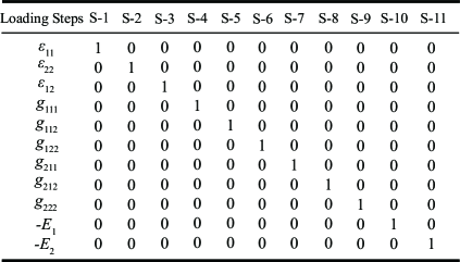
Figure 1: Loading steps for macroscopic constitutive tangents calculation

4 Numerical implementation

4.1 $C^{1}$ finite elements

$C^{1}$ finite elements, that were initially developed for modeling plate structures, are well suited to second-order homogenization of flexoelectricity. It is easier to impose the periodic boundary conditions due to the presence of displacement derivatives in the nodal degrees of freedom. A review and catalog of the $C^{1}$ finite elements can be found in [37]. The Argyris triangle [38] is a well-known $h$-version $C^{1}$ conforming element. The degrees of freedom include all second-order derivatives on vertices and normal derivatives at mid-side nodes (Fig. 3), with complete fifth-order polynomial interpolation functions. However, the normal derivatives at midsides are undesirable and are eliminated by interpolating the normal derivative at the mid-side nodes from the derivatives at the corner nodes, resulting in the $C^{1}$ Bell triangle element [39]. The displacement field still varies as a complete quintic inside the element, and the normal derivative along the edges of the element is constrained to be cubic [40]. The governing equation of flexoelectricity is a fourth-order partial differential equation, so the Bell triangle element satisfies the requirements of completeness and compatibility. The shape functions for the Bell triangle were given by Dasgupta and Sengupta [29]. The utility of the Bell triangle was proven in a series of studies on gradient elasticity problems [40, 41, 42].

The Bell triangle is applied here as shown in Fig. 3. Each node has eighteen degrees of freedom, which are displacement and electric potential and their first and second-order derivatives.

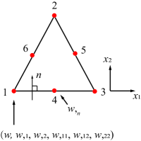
Figure 2: Argyris triangle

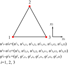
Figure 3: Bell triangle

In the absence of $E_{i,j}$, $\bar{r}_{i}$ and $\bar{v}_{i}$, the weak form of formulation for flexoelectricity is written as

$$\int_{v}(\boldsymbol{\sigma}:\delta\boldsymbol{\varepsilon}+\boldsymbol{\tau}\vdots\delta\boldsymbol{g}-\boldsymbol{D}\cdot\delta\boldsymbol{E})dv=\int_{v}(\boldsymbol{f}^{b}\cdot\delta\boldsymbol{u})dv+\int_{\varGamma_{t}}(\bar{\boldsymbol{t}}\cdot\delta\boldsymbol{u})d\varGamma-\int_{v}{\rho^{f}}\delta\phi dv-\int_{\varGamma_{D}}\omega\delta\phi d\varGamma$$ (44)

The displacement $\boldsymbol{u}$ and electric potential $\phi$ fields, as well as their derivatives, can be approximated according to

$$\boldsymbol{u}=\boldsymbol{N}_{u}\boldsymbol{v}^{e},\;\phi=\boldsymbol{N}_{\phi}\boldsymbol{\varphi}^{e}$$ (45)

$$\boldsymbol{\varepsilon}=\boldsymbol{B}_{u}\boldsymbol{v}^{e},\;\boldsymbol{g}=\boldsymbol{H}_{u}\boldsymbol{v}^{e},\;-\boldsymbol{E}=\boldsymbol{B}_{\phi}\boldsymbol{\varphi}^{e}$$ (46)

where $\boldsymbol{\varepsilon}=(\varepsilon_{11},\varepsilon_{22},\varepsilon_{12})^{T}$, $\boldsymbol{g}=(g_{111},g_{112},g_{122},g_{211},g_{212},g_{222})^{T}$, $-\boldsymbol{E}=(-E_{1},-E_{2})^{T}$. $\boldsymbol{N}_{u}$, $\boldsymbol{N}_{\phi}$ are the shape function matrix, and $\boldsymbol{v}^{e}$ and $\boldsymbol{\varphi}^{e}$ are the nodal degrees of freedom. $\boldsymbol{B}_{u}$, $\boldsymbol{B}_{\phi}$, and $\boldsymbol{H}_{u}$ are matrices containing the gradient and Hessian of the corresponding shape functions.

Substituting Eqs. (45)–(46) into Eq. (44) yields

$$\begin{bmatrix}\boldsymbol{K}_{uu}&\boldsymbol{K}_{u\phi}\\ \boldsymbol{K}_{\phi u}&\boldsymbol{K}_{\phi\phi}\\ \end{bmatrix}\begin{bmatrix}\boldsymbol{v}\\ \boldsymbol{\varphi}\\ \end{bmatrix}=\begin{bmatrix}\boldsymbol{F}_{v}\\ \boldsymbol{F}_{\varphi}\\ \end{bmatrix}$$ (47)

where

$$\boldsymbol{K}_{uu}=\sum_{e}\int_{v_{e}}(\boldsymbol{B}^{T}_{u}\boldsymbol{C}\boldsymbol{B}_{u}+l^{2}\boldsymbol{H}^{T}_{u}\boldsymbol{Q}\boldsymbol{H}_{u})dv$$ (48)

$$\boldsymbol{K}_{u\phi}=\sum_{e}\int_{v_{e}}(\boldsymbol{B}^{T}_{u}\boldsymbol{e}\boldsymbol{B}_{\phi}+\boldsymbol{H}^{T}_{u}\boldsymbol{f}^{T}\boldsymbol{B}_{\phi})dv$$ (49)

$$\boldsymbol{K}_{\phi u}=\sum_{e}\int_{v_{e}}(\boldsymbol{B}^{T}_{\phi}\boldsymbol{e}^{T}\boldsymbol{B}_{u}+\boldsymbol{B}^{T}_{\phi}\boldsymbol{f}\boldsymbol{H}_{u})dv$$ (50)

$$\boldsymbol{K}_{\phi\phi}=\sum_{e}\int_{v_{e}}(\boldsymbol{B}^{T}_{\phi}(-\boldsymbol{\kappa})\boldsymbol{B}_{\phi})dv$$ (51)

$$\boldsymbol{F}_{u}=\sum_{e}\int_{v_{e}}(\boldsymbol{N}^{T}_{u}\boldsymbol{f}^{b})dv+\sum_{e}\int_{\varGamma_{t}}(\boldsymbol{N}^{T}_{u}\bar{\boldsymbol{t}})d\varGamma$$ (52)

$$\boldsymbol{F}_{\phi}=-\sum_{e}\int_{v_{e}}(\boldsymbol{N}^{T}_{\phi}\rho^{f})dv-\sum_{e}\int_{\varGamma_{D}}(\boldsymbol{N}^{T}_{\phi}\omega)d\varGamma$$ (53)

Moreover, $\boldsymbol{C}$, $\boldsymbol{Q}$, $\boldsymbol{\kappa}$, $\boldsymbol{e}$ and $\boldsymbol{f}$ can be written in matrix format as

$$\boldsymbol{C}=\begin{bmatrix}\lambda+2G&\lambda&0\\ \lambda&\lambda+2G&0\\ 0&0&4G\end{bmatrix},\;\boldsymbol{\kappa}=\begin{bmatrix}\kappa_{11}&0\\ 0&\kappa_{33}\end{bmatrix}$$ (54)

$$\boldsymbol{e}^{T}=\begin{bmatrix}0&0&2e_{15}\\ e_{31}&e_{33}&0\end{bmatrix},\;\boldsymbol{f}=\begin{bmatrix}f_{1}+2f_{2}&0&f_{1}&0&2f_{2}&0\\ 0&2f_{2}&0&f_{1}&0&f_{1}+2f_{2}\end{bmatrix}$$ (55)

$$\boldsymbol{Q}=\begin{bmatrix}\lambda+2G&0&0&0&\lambda&0\\ 0&\lambda+3G&0&G&0&\lambda\\ 0&0&G&0&G&0\\ 0&G&0&G&0&0\\ \lambda&0&G&0&\lambda+3G&0\\ 0&\lambda&0&0&0&\lambda+2G\end{bmatrix}$$ (56)

4.2 Periodic boundary conditions

The twelve displacement-related degrees of freedom per node are expressed as $\boldsymbol{u}_{g}$ and the six electric potential-related degrees of freedom are denoted as $\boldsymbol{\phi}_{g}$. $\boldsymbol{u}_{g}$ and $\boldsymbol{\phi}_{g}$ of nodes on the RVE boundary can be rewritten into the matrix form as

$$\boldsymbol{u}_{g}=\boldsymbol{W}\boldsymbol{\varepsilon}_{M}+\boldsymbol{S}\boldsymbol{g}_{M}+\boldsymbol{r}_{u}$$ (57)

$$\boldsymbol{\phi}_{g}=\boldsymbol{L}(-\boldsymbol{E}_{M})+\boldsymbol{r}_{\phi}$$ (58)

where

$$\boldsymbol{W}=\begin{bmatrix}x_{1}&0&x_{2}\\ 1&0&0\\ 0&0&1\\ 0&0&0\\ 0&0&0\\ 0&0&0\\ 0&x_{2}&x_{1}\\ 0&0&1\\ 0&1&0\\ 0&0&0\\ 0&0&0\\ 0&0&0\end{bmatrix},\;\boldsymbol{S}=\begin{bmatrix}\frac{1}{2}x^{2}_{1}&x_{1}x_{2}&\frac{1}{2}x^{2}_{2}&0&0&0\\ x_{1}&x_{2}&0&0&0&0\\ 0&x_{1}&x_{2}&0&0&0\\ 1&0&0&0&0&0\\ 0&1&0&0&0&0\\ 0&0&1&0&0&0\\ 0&0&0&\frac{1}{2}x^{2}_{1}&x_{1}x_{2}&\frac{1}{2}x^{2}_{2}\\ 0&0&0&x_{1}&x_{2}&0\\ 0&0&0&0&x_{1}&x_{2}\\ 0&0&0&1&0&0\\ 0&0&0&0&1&0\\ 0&0&0&0&0&1\end{bmatrix},\;\boldsymbol{L}=\begin{bmatrix}x_{1}&x_{2}\\ 1&0\\ 0&1\\ 0&0\\ 0&0\\ 0&0\\ \end{bmatrix}$$ (59)

Here $x_{1}$ and $x_{2}$ denote the coordinates of the node. Using the periodicity according to relations (25)-(27) leads to the equations

$$\boldsymbol{u}_{gR}-\boldsymbol{u}_{gL}=(\boldsymbol{W}_{R}-\boldsymbol{W}_{L})\boldsymbol{\varepsilon}_{M}+(\boldsymbol{S}_{R}-\boldsymbol{S}_{L})\boldsymbol{g}_{M},\;\boldsymbol{u}_{gT}-\boldsymbol{u}_{gB}=(\boldsymbol{W}_{T}-\boldsymbol{W}_{B})\boldsymbol{\varepsilon}_{M}+(\boldsymbol{S}_{T}-\boldsymbol{S}_{B})\boldsymbol{g}_{M}$$ (60)

$$\boldsymbol{\phi}_{gR}-\boldsymbol{\phi}_{gL}=(\boldsymbol{L}_{R}-\boldsymbol{L}_{L})(-\boldsymbol{E}_{M}),\;\boldsymbol{\phi}_{gT}-\boldsymbol{\phi}_{gB}=(\boldsymbol{L}_{T}-\boldsymbol{L}_{B})(-\boldsymbol{E}_{M})$$ (61)

The above periodic condition can be called the gradient generalized periodic condition (PBC) [20]. There is another boundary condition-gradient displacement periodic condition (DBC), where microfluctuations on the RVE boundaries are suppressed, so the displacement and electric potential field of nodes on the RVE boundary are then written as

$$\boldsymbol{u}_{g}=\boldsymbol{W}\boldsymbol{\varepsilon}_{M}+\boldsymbol{S}\boldsymbol{g}_{M}$$ (62)

$$\boldsymbol{\phi}_{g}=\boldsymbol{L}(-\boldsymbol{E}_{M})$$ (63)

4.3 The second-order multiscale solution scheme

The second-order multiscale solution scheme is shown in Fig. 4. The second-order homogenization procedure for flexoelectricity is implemented with ABAQUS. $C^{1}$ triangular finite element is realized using the user element subroutine UEL, and user subroutine UVARM with “dummy” elements are used for postprocessing the field results of user-defined elements. The field results are obtained as output in TECPLOT format for visualization. As user subroutine UVARM cannot be used with linear perturbation procedure in ABAQUS, the macroscopic constitutive tangents are calculated with perturbation analysis in the general step. The periodic boundary conditions are imposed with linear constraint equations in ABAQUS. As this study is on flexoelectric structures under small elastic deformation, the macro-micro scale transition (Fig. 5) is carried out only once.

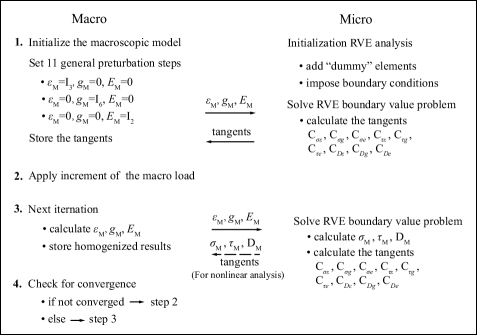
Figure 4: The second-order multiscale solution scheme

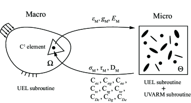
Figure 5: The macro-micro scale transition

5 Numerical examples

5.1 Material equivalent parameter analysis of a square plate with holes

For the sake of comparison, only the representative material equivalent parameters of the flexoelectric microstructure are analyzed, and the equivalent parameters in the following examples are all expressed by the two-index notation. Taking the square plate with holes as an example, the effects of intrinsic length, microscale model size, porosity, and void distribution on the equivalent parameters are investigated. Furthermore, two different boundary conditions (PBC and DBC) are also compared. The material properties of microscale structure are listed in Tab. 1 based on [24, 23].

Table 1: Material properties ($[\lambda,G]=\rm{GPa}$, $[e]=\rm{C/m^{2}}$, $[\kappa]=\rm{nC/Vm}$, $[f]=\rm{\mu C/m}$)

$\lambda$	$G$	$e_{31}$	$e_{33}$	$e_{15}$	$k_{11}$	$k_{33}$	$f_{1}$	$f_{2}$
$179$	$54$	$-2.7$	$3.65$	$21.3$	$12.5$	$14.4$	$1$	$1$

5.1.1 The effects of intrinsic length and microscale model size

The expression of intrinsic length can be given by the self-consistent estimate [43] and its calculation is beyond the scope of this paper. The intrinsic length in flexoelectricity analysis is taken as the model size multiplied by a factor smaller than one [24, 25], but the value of the factor is not definite.

The microscale model with a side length of 1 $\mu\rm{m}$ is shown in Fig. 6. The effects of intrinsic length on the equivalent parameters of microstructure are shown in Fig. 8. The parameters are normalized by dividing the corresponding material property in Tab. 1 to aid comparison. One can observe that the dielectric and flexoelectric coefficients decrease and the elastic and piezoelectric coefficients increase with the increase of intrinsic length, while all the coefficients remain unchanged when the intrinsic length is over 0.5 $\mu\rm{m}$. The effects of boundary conditions, i.e. PBC and DBC, on the results are shown in Fig. 8. The equivalent elastic coefficients remain quite similar irrespective of the considered boundary conditions, while the dielectric, piezoelectric, and flexoelectric coefficients differ noticeably under DBC.

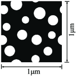
Figure 6: The mircroscale model with holes

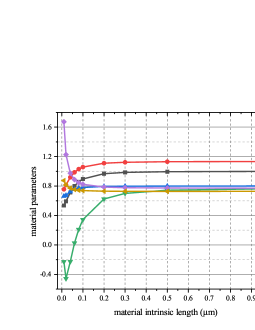
Figure 7: Material parameters of different intrinsic length l

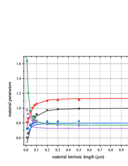
Figure 8: Material parameters of different intrinsic length l with different boundary conditions

Keeping the intrinsic length constant ($1\rm{\mu m}$), the effects of microscale model size are shown in Fig. 10. The elastic and piezoelectric coefficients decrease, while the dielectric and flexoelectric coefficients increase with the increase of microscale model size. On the other hand, the dielectric, piezoelectric, and flexoelectric coefficients are also larger under DBC compared to PBC, as in Fig. 10.

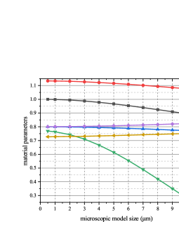
Figure 9: Material parameters of different microscopic model sizes

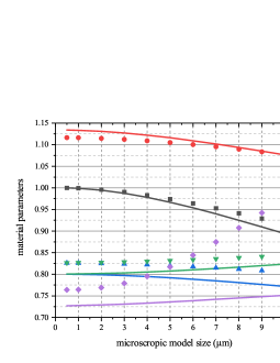
Figure 10: Material parameters of different microscopic model sizes with different boundary conditions

5.1.2 The effects of porosity and void distribution

The side length of the model and intrinsic length are $1\ \mu\rm{m}$, and PBC is set as the boundary condition. The variation of the equivalent material parameters is linearly related to the porosity as shown in Fig. 12. As the porosity increases, the dielectric, piezoelectric and flexoelectric coefficients decrease, and the elastic coefficient $C_{33}$ increases, while the elastic coefficient $C_{11}$ remains almost unchanged. It should be noted that when the porosity is zero, the equivalent material parameters are the same as the microscopic material, which is consistent with intuition. According to Fig. 12, the equivalent flexoelectric parameter is more obviously impacted by the void distribution than other parameters. Compared with void distribution, the influence of shape and topology of microstructure on the equivalent material parameters will be greater, which needs further study.

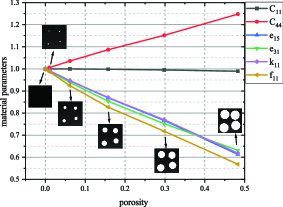
Figure 11: Material parameters of different porosities

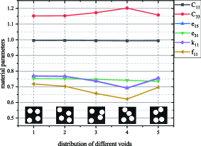
Figure 12: Material parameters of different distribution of holes

5.2 Creating materials with piezoelectric behaviour without using piezoelectric materials

Flexoelectricity can be exploited to design piezoelectric effects without using piezoelectric materials by seeking to induce strain gradients [44, 45]. One method is to introduce a triangular hole in a sheet, then a net nonzero polarization exists under uniform stretching. It is to be noted that, the average polarization remains zero if the shape of the hole is circular, as shown in Fig. 14. In this paper, similar methods are applied in the microscale model to create equivalent piezoelectric coefficients in the absence of piezoelectric materials.

5.2.1 Two-scale linear analysis of a uniaxial tensioned square plate

The macroscale model is a square plate subjected to uniaxial tension, and the microscale model is a square with a triangular hole in the center (Fig. 14). The material properties are similar to the ones used in the previous examples as listed in Tab. 1, except that the values of piezoelectric coefficients are considered to be zero. The intrinsic length is set to be 1 $\rm{\mu m}$.

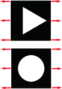
Figure 13: Piezoelectric nanocomposites without using piezoelectric materials [44]

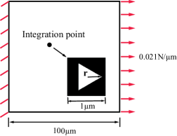
Figure 14: Macroscopic and microscopic models

Fig. 16 gives piezoelectric coefficients with different hole sizes measured by the radius $r$ of the inscribed circle of a triangle. The piezoelectric coefficients $e_{11}$, $e_{12}$, $e_{23}$ generally increase as $r$ increases, while $e_{13}$, $e_{21}$, $e_{22}$ are almost zero. It is noteworthy that the equivalent piezoelectric coefficients are calculated to be zero when the hole is a circle, regardless of the hole size, which is consistent with the discussion in [44].

The electric displacement field $D_{1}$ of the macro model with $r=0.4\ \mu\rm{m}$ in the microstructure is shown in Fig. 16. The electric displacement field $D_{1}$ of the microstructure which corresponds to one integration point of element 1 in the macro model is also given in the figure. The calculation procedure has been described in Fig. 4, and the macro-micro scale transition is carried out only once because of the linear elastic analysis.

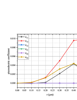
Figure 15: Equivalent piezoelectric coefficients ($\rm{C/m^{2}}$) of different hole sizes

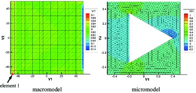
Figure 16: $D_{1}$ of the macroscale and microscale model ($\rm{C/m^{2}}$)

5.2.2 Creating piezoelectric materials with flexoelectric composites

Similarly, we can design piezoelectric materials with flexoelectric composites by distributing flexoelectric inclusions (B) in the dielectric matrix (M), as shown in Fig. 17. The material properties of the inclusions are listed in Tab. 1, the side length is $1\ \mu\rm{m}$, and the intrinsic length is ignored. The dielectric coefficients of the matrix are the same as the inclusions, but the flexoelectric coefficients are zero. To induce the strain gradients, the elastic tensor of the matrix is adjusted and set to be the inclusions’ elastic tensor multiplied by a factor less than 1. As the factor varies between 0 and 1, the homogenized piezoelectric coefficients vary as shown in Fig. 19. when the factor is 1 or 0, the homogenized piezoelectric coefficients are nearly zero because the strain gradient is too small (factor=1) or the connection between the inclusions is extremely weak (factor=0). The ideal factor is around 0.2.

Moreover, the size-dependent behaviour of flexoelectricity can be used to enhance the homogenized piezoelectric coefficients. By reducing the size of the microscale composite structure, from the micron-scale to the nanoscale, the homogenized piezoelectric coefficients increase significantly even though the elastic tensor factor is 1 (Fig. 19). Interestingly, we can get similar results by increasing the flexoelectric coefficients of the inclusions without shrinking the microstructure size. The same homogenized piezoelectric coefficients can be obtained simply by increasing the flexoelectric coefficients of the inclusions by a factor of $f_{k}$ (Fig. 19), instead of scaling the microstructure down when regardless of the intrinsic length, which are consistent with the dimensional analysis. The results in Fig. 19 illustrate the size-dependent behaviour of flexoelectricity in another way.

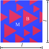
Figure 17: Flexoelectric composites

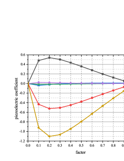
Figure 18: Homogenized piezoelectric coefficients ($\rm{C/m^{2}}$) of different factors

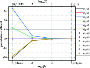
Figure 19: Homogenized piezoelectric coefficients ($\rm{C/m^{2}}$) of different micromodel sizes $l$ and factors $f_{k}$

Remark: the self-consistency of the proposed method is reflected in four aspects: 1. The equivalent material parameters are the same as the microscopic material when the porosity is zero (Fig. 11); 2. The equivalent piezoelectric coefficients are calculated to be zero when the hole is a circle; 3. The homogenized piezoelectric coefficients are nearly zero when the elastic tensor factor of the matrix is 1 or 0 (Fig. 18); 4. The same homogenized piezoelectric coefficients can be obtained by increasing the flexoelectric coefficients of the inclusions or shrinking the microstructure size (Fig. 19).

6 Conclusion

The computational second-order homogenization strategy of flexoelectric composites has been presented. The framework was implemented with $C^{1}$ triangular finite elements based on the secondary development of ABAQUS via user subroutines UEL and UVARM. Compared to the asymptotic expansion method, the homogenized electromechanical properties can be computed using perturbation analysis without complicated mathematical derivations. The influence of intrinsic length, micromodel size, and the two boundary conditions on the effective coefficients of flexoelectric microstructure are discussed. The influence of porosity and void distribution in the microstructure on the equivalent piezoelectric coefficients are also studied. The homogenized piezoelectric coefficients by introducing triangular voids or flexoelectric inclusions in the microstructure are determined. In this work, we restrict the computational second-order homogenization scheme to the linear 2D case, however, considering nonlinearity and extension to 3D problems are straightforward.

References

References

- Majdoub et al. [2008] M. Majdoub, P. Sharma, T. Cagin, Enhanced size-dependent piezoelectricity and elasticity in nanostructures due to the flexoelectric effect, Physical Review B 77 (12) (2008) 125424.
- Nguyen et al. [2013] T. D. Nguyen, S. Mao, Y.-W. Yeh, P. K. Purohit, M. C. McAlpine, Nanoscale flexoelectricity, Advanced Materials 25 (7) (2013) 946–974.
- Zubko et al. [2013] P. Zubko, G. Catalan, A. K. Tagantsev, Flexoelectric effect in solids, Annual Review of Materials Research 43.
- Yudin and Tagantsev [2013] P. Yudin, A. Tagantsev, Fundamentals of flexoelectricity in solids, Nanotechnology 24 (43) (2013) 432001.
- Wang et al. [2019] B. Wang, Y. Gu, S. Zhang, L.-Q. Chen, Flexoelectricity in solids: Progress, challenges, and perspectives, Progress in Materials Science 106 (2019) 100570.
- Arias et al. [2022] I. Arias, G. Catalan, P. Sharma, The emancipation of flexoelectricity, 2022.
- Mocci et al. [2021] A. Mocci, J. Barceló-Mercader, D. Codony, I. Arias, Geometrically polarized architected dielectrics with apparent piezoelectricity, Journal of the Mechanics and Physics of Solids 157 (2021) 104643.
- Zhang et al. [2016] C. Zhang, L. Zhang, X. Shen, W. Chen, Enhancing magnetoelectric effect in multiferroic composite bilayers via flexoelectricity, Journal of Applied Physics 119 (13) (2016) 134102.
- Zhang et al. [2021] M. Zhang, D. Yan, J. Wang, L.-H. Shao, Ultrahigh flexoelectric effect of 3D interconnected porous polymers: modelling and verification, Journal of the Mechanics and Physics of Solids 151 (2021) 104396.
- McBride et al. [2020] A. McBride, D. Davydov, P. Steinmann, Modelling the flexoelectric effect in solids: a micromorphic approach, Computer Methods in Applied Mechanics and Engineering 371 (2020) 113320.
- Guinovart-Sanjuán et al. [2019] D. Guinovart-Sanjuán, J. Merodio, J. C. López-Realpozo, K. Vajravelu, R. Rodríguez-Ramos, R. Guinovart-Díaz, J. Bravo-Castillero, F. J. Sabina, Asymptotic homogenization applied to flexoelectric rods, Materials 12 (2) (2019) 232.
- Mohammadi et al. [2014] P. Mohammadi, L. Liu, P. Sharma, A theory of flexoelectric membranes and effective properties of heterogeneous membranes, Journal of Applied Mechanics 81 (1).
- Sharma et al. [2007] N. Sharma, R. Maranganti, P. Sharma, On the possibility of piezoelectric nanocomposites without using piezoelectric materials, Journal of the Mechanics and Physics of Solids 55 (11) (2007) 2328–2350.
- Geers and Yvonnet [2016] M. Geers, J. Yvonnet, Multiscale modeling of microstructure–property relations, MRS Bulletin 41 (8) (2016) 610–616.
- Geers et al. [2010] M. G. Geers, V. G. Kouznetsova, W. Brekelmans, Multi-scale computational homogenization: Trends and challenges, Journal of computational and applied mathematics 234 (7) (2010) 2175–2182.
- Kaczmarczyk et al. [2008] Ł. Kaczmarczyk, C. J. Pearce, N. Bićanić, Scale transition and enforcement of RVE boundary conditions in second-order computational homogenization, International Journal for Numerical Methods in Engineering 74 (3) (2008) 506–522.
- Kouznetsova et al. [2004] V. Kouznetsova, M. G. Geers, W. Brekelmans, Multi-scale second-order computational homogenization of multi-phase materials: a nested finite element solution strategy, Computer methods in applied Mechanics and Engineering 193 (48-51) (2004) 5525–5550.
- Lesičar et al. [2014] T. Lesičar, Z. Tonković, J. Sorić, A second-order two-scale homogenization procedure using macrolevel discretization, Computational mechanics 54 (2) (2014) 425–441.
- Lesičar et al. [2016] T. Lesičar, J. Sorić, Z. Tonković, Large strain, two-scale computational approach using C1 continuity finite element employing a second gradient theory, Computer methods in applied mechanics and engineering 298 (2016) 303–324.
- Lesičar et al. [2017] T. Lesičar, Z. Tonković, J. Sorić, Two-scale computational approach using strain gradient theory at microlevel, International Journal of Mechanical Sciences 126 (2017) 67–78.
- Lesičar [2015] T. Lesičar, Multiscale modeling of heterogeneous materials using second-order homogenization, Ph.D. thesis, University of Zagreb. Faculty of Mechanical Engineering and Naval Architecture., 2015.
- Ghasemi et al. [2017] H. Ghasemi, H. S. Park, T. Rabczuk, A level-set based IGA formulation for topology optimization of flexoelectric materials, Computer Methods in Applied Mechanics and Engineering 313 (2017) 239–258.
- Nanthakumar et al. [2017] S. Nanthakumar, X. Zhuang, H. S. Park, T. Rabczuk, Topology optimization of flexoelectric structures, Journal of the Mechanics and Physics of Solids 105 (2017) 217–234.
- Deng et al. [2017] F. Deng, Q. Deng, W. Yu, S. Shen, Mixed finite elements for flexoelectric solids, Journal of Applied Mechanics 84 (8).
- Mao et al. [2016] S. Mao, P. K. Purohit, N. Aravas, Mixed finite-element formulations in piezoelectricity and flexoelectricity, Proceedings of the Royal Society A: Mathematical, Physical and Engineering Sciences 472 (2190) (2016) 20150879.
- Poya et al. [2019] R. Poya, A. J. Gil, R. Ortigosa, R. Palma, On a family of numerical models for couple stress based flexoelectricity for continua and beams, Journal of the Mechanics and Physics of Solids 125 (2019) 613–652.
- He et al. [2019] B. He, B. Javvaji, X. Zhuang, Characterizing flexoelectricity in composite material using the element-free Galerkin method, Energies 12 (2) (2019) 271.
- Yvonnet and Liu [2017] J. Yvonnet, L. Liu, A numerical framework for modeling flexoelectricity and Maxwell stress in soft dielectrics at finite strains, Computer Methods in Applied Mechanics and Engineering 313 (2017) 450–482.
- Dasgupta and Sengupta [1990] S. Dasgupta, D. Sengupta, A higher-order triangular plate bending element revisited, International Journal for Numerical Methods in Engineering 30 (3) (1990) 419–430.
- Maranganti et al. [2006] R. Maranganti, N. Sharma, P. Sharma, Electromechanical coupling in nonpiezoelectric materials due to nanoscale nonlocal size effects: Green’s function solutions and embedded inclusions, Physical Review B 74 (1) (2006) 014110.
- Sharma et al. [2010] N. Sharma, C. Landis, P. Sharma, Piezoelectric thin-film superlattices without using piezoelectric materials, Journal of Applied Physics 108 (2) (2010) 024304.
- Abdollahi et al. [2015] A. Abdollahi, D. Millán, C. Peco, M. Arroyo, I. Arias, Revisiting pyramid compression to quantify flexoelectricity: A three-dimensional simulation study, Physical Review B 91 (10) (2015) 104103.
- Shen and Hu [2010] S. Shen, S. Hu, A theory of flexoelectricity with surface effect for elastic dielectrics, Journal of the Mechanics and Physics of Solids 58 (5) (2010) 665–677.
- Hu and Shen [2010] S. Hu, S. Shen, Variational principles and governing equations in nano-dielectrics with the flexoelectric effect, Science China Physics, Mechanics and Astronomy 53 (8) (2010) 1497–1504.
- Hill [1963] R. Hill, Elastic properties of reinforced solids: some theoretical principles, Journal of the Mechanics and Physics of Solids 11 (5) (1963) 357–372.
- Schröder and Keip [2012] J. Schröder, M.-A. Keip, Two-scale homogenization of electromechanically coupled boundary value problems, Computational mechanics 50 (2) (2012) 229–244.
- Hrabok and Hrudey [1984] M. Hrabok, T. Hrudey, A review and catalogue of plate bending finite elements, Computers & Structures 19 (3) (1984) 479–495.
- Argyris et al. [1968] J. H. Argyris, I. Fried, D. W. Scharpf, The TUBA family of plate elements for the matrix displacement method, The Aeronautical Journal 72 (692) (1968) 701–709.
- Bell [1969] K. Bell, A refined triangular plate bending finite element, International journal for numerical methods in engineering 1 (1) (1969) 101–122.
- Zervos et al. [2001] A. Zervos, P. Papanastasiou, I. Vardoulakis, A finite element displacement formulation for gradient elastoplasticity, International Journal for Numerical Methods in Engineering 50 (6) (2001) 1369–1388.
- Zervos et al. [2009] A. Zervos, S.-A. Papanicolopulos, I. Vardoulakis, Two finite-element discretizations for gradient elasticity, Journal of engineering mechanics 135 (3) (2009) 203–213.
- Manzari and Yonten [2013] M. T. Manzari, K. Yonten, C1 finite element analysis in gradient enhanced continua, Mathematical and Computer Modelling 57 (9-10) (2013) 2519–2531.
- Aifantis [2000] E. C. Aifantis, Gradient aspects of crystal plasticity at micro and macro scales, in: Key Engineering Materials, vol. 177, Trans Tech Publ, 805, 2000.
- Krichen and Sharma [2016] S. Krichen, P. Sharma, Flexoelectricity: a perspective on an unusual electromechanical coupling, Journal of Applied Mechanics 83 (3).
- Deng et al. [2014] Q. Deng, L. Liu, P. Sharma, Flexoelectricity in soft materials and biological membranes, Journal of the Mechanics and Physics of Solids 62 (2014) 209–227.