Astronomy Letters, 2023, Vol. 49, No. 9, pp. 493–500.

Estimation of the Galactocentric Distance of the Sun from

Cepheids Close to the Solar Circle

V. V. Bobylev

Pulkovo Astronomical Observatory, Russian Academy of Sciences, St. Petersburg, 196140 Russia

Based on Cepheids located near the solar circle, we have determined the Galactocentric distance of the Sun $R_{0}$ and the Galactic rotation velocity at the solar distance $V_{0}$. For our analysis we used a sample of $\sim$200 classical Cepheids from the catalogue by Skowron et al. (2019), where the distances to them were determined from the period–luminosity relation. For these stars the proper motions and line-of-sight velocities were taken from the Gaia DR3 catalogue. The values of $R_{0}$ found lie within the range [7.8–8.3] kpc, depending on the heliocentric distance of the sample stars, on the adopted solar velocity relative to the local standard of rest, and on whether or not the perturbations caused by the Galactic spiral density wave are taken into account. The dispersion of the $R_{0}$ estimates is $\sim$2 kpc. Similarly, the values of $V_{0}$ lie within the range [240–270] km s^-1 with a dispersion of the estimates of 70–90 km s^-1. We consider the following estimates to be the final ones: $R_{0}=8.24\pm 0.20$ kpc and $V_{0}=268\pm 8$ km s^-1 found by taking into account the perturbations from the Galactic spiral density wave.

INTRODUCTION

The Galactocentric distance of the Sun $R_{0}$ is an important parameter for studying the structure, kinematics, and dynamics of the Galaxy. Various methods of estimating this quantity are known. According to Reid (1993), such measurements can be divided into direct, secondary, and indirect. Bland-Hawthorn and Gerhard (2016) propose to divide such measurements into direct, model-dependent, and secondary. Nikiforov (2004) proposed a special classification with the division of measurements into three classes, depending on the type of measurements, the type of $R_{0}$ estimates, and the type of reference objects.

A truly direct method is to determine the absolute trigonometric parallax of an object located near the Galactic center. Based on VLBI observations of several maser sources in the region Sgr B2, Reid et al. (2009) obtained an estimate of $R_{0}=7.9^{+0.8}_{-0.7}$ kpc by this method. The dynamical parallax method can also be assigned to the direct ones. At present, an analysis of the orbital motion of stars around the central supermassive black hole allows $R_{0}$ to be estimated by this method with a relative error of about 0.3% (Abuter et al. 2019). According to one of the latest determinations of the GRAVITY Collaboration, $R_{0}=8275\pm 9_{\rm stat.}\pm 33_{\rm sys.}$ pc (Abuter et al. 2021).

Such variable stars as classical Cepheids, type II Cepheids, and RR Lyrae variables are important for estimating $R_{0}$. A high accuracy of the distance estimates for these variables is possible owing to the period–luminosity relation (Leavitt 1908; Leavitt and Pickering 1912) and the period–Wesenheit relation (Madore 1982), which have currently been well calibrated using highly accurate trigonometric parallaxes of stars (Ripepi et al. 2019).

Type II Cepheids and RR Lyrae variables are distributed over the entire Galaxy. Relatively younger classical Cepheids are distributed over the entire Galactic disk. Their geometric and kinematic properties are used to estimate $R_{0}$. For example, the R0 estimation methods based on the assumption about a symmetric distribution of Cepheids in the Galactic bulge or a symmetric distribution of globular cluster member variable stars in the Galaxy are known. The estimates of $R_{0}$ are quite often obtained by analyzing the Galactic rotation curve, where $R_{0}$ acts as a sought-for unknown, along with other parameters. However, the estimates of $R_{0}$ are obtained by analyzing the Galactic rotation curve not only from Cepheids, but also from other Galactic disk objects — masers, OB stars, open star clusters, etc.

In addition to the first-class distances to Cepheids, it is important to have their highly accurate proper motions and line-of-sight velocities. From this point of view, of great interest is the Gaia space experiment (Prusti et al. 2016), which is devoted to the determination of highly accurate trigonometric parallaxes, proper motions, and a number of photometric characteristics for more than 1.5 billion stars. In the recently published GaiaDR3 version (Vallenari et al. 2022), the line-of-sight velocities of stars were improved significantly — the previously measured values were refined and the new ones were determined for a large number of stars. At the same time, the trigonometric parallaxes and proper motions of stars were copied from the previous version of the Gaia EDR3 catalogue (Gaia Early Data Release 3, Brown et al. 2021).

Various authors regularly perform reviews of individual $R_{0}$ estimates with the derivation of their mean. For example, Nikiforov (2004) found $R_{0}=7.9\pm 0.2$ kpc based on 65 original measurements from 1974 to 2004, Malkin (2013) calculated the mean $R_{0}=8.0\pm 0.25$ kpc by analyzing 53 individual estimates from 1992 to 2011, and Bobylev and Bajkova (2021) found $R_{0}=8.1\pm 0.1$ kpc based on 56 measurements from 2011 to 2021.

The goal of this paper is to estimate $R_{0}$ and the circular rotation velocity of the Galaxy at the solar distance $V_{0}$ using a large sample of classical Cepheids located near the solar circle. For this purpose, we use Cepheids from the catalogue by Skowron et al. (2019), where the distances to them were determined from the period–luminosity relation with a mean error of about 5%. We took the proper motions and line-of-sight velocities of these Cepheids from the Gaia DR3 catalogue. We applied a peculiar method of estimating $R_{0}$ and $V_{0}$ based on the analysis of objects close to the solar circle. The method is interesting in that $R_{0}$ and $V_{0}$ can be estimated even from one star located on the solar circle.

METHOD

To estimate the Galactocentric distance of the Sun $R_{0}$ and the circular rotation velocity of the Galaxy at the solar distance $V_{0}$ using objects located near the solar circle, we know a method (see, e.g., Schechter et al. 1992) that we will call the classic one:

$$R_{0}={r\over 2\cos l},\quad V_{0}=-{V_{l}\over 2\cos l},$$ (1)

where $r$ is the heliocentric distance of the star and $V_{l}$ is the velocity directed along the Galactic longitude ($V_{l}=4.74r\mu_{l}\cos b$). Here, the line-of-sight velocity $V_{r}$ of each star lying on the solar circle is assumed to be zero.

Sofue et al. (2011) proposed the following modification of the classic method:

$$R_{0}={r\over 2\cos l}(1-d/r),$$ (2)

$$V_{0}=-{V_{l}\over 2\cos l}(1-d/r)+V_{r}\cot l,$$ (3)

where $d$ is the distance along the line of sight to the star from the solar circle,

$$d=-{V_{r}\over A\sin 2l},$$ (4)

$A$ is the Oort constant whose value in this paper is taken to be $A=15$ km s^-1 kpc^-1. The velocities $V_{r}$ and $V_{l}$ should be given relative to the local standard of rest. To reduce the observed heliocentric velocities of the stars to the local standard of rest, we use two sets of velocities. In the first case, we take the velocities from Schönrich et al. (2010):

$$(U,V,W)_{\odot}=(11.10,12.24,7.25)~{}\hbox{km s${}^{-1}$},$$ (5)

while in the second case we use the velocities found from a large sample of classical Cepheids in Bobylev and Bajkova (2023):

$$(U,V,W)_{\odot}=(9.39,15.96,6.88)~{}\hbox{km s${}^{-1}$}.$$ (6)

The velocities (6) are close to the corresponding velocities of the so-called standard solar apex $(U,V,W)_{\odot}=(10.3,15.3,7.7)$ km s^-1 that were used by Sofue et al. (2011) to analyze the masers Onsala 1 and Onsala 2N. When we repeated their calculations, it was found that the estimate of $R_{0}$ depends fairly strongly on the adopted solar velocity relative to the local standard of rest. Therefore, in this paper we use both sets of such velocities.

The errors in $R_{0}$ and $V_{0}$ are estimated in accordance with the following formulas:

$$\delta R_{0}={1\over 2\cos l}\left[\delta r^{2}+\left({\delta V_{r}\over A\sin 2l}\right)^{2}\right]^{1/2},$$ (7)

$$\begin{array}[]{lll}\displaystyle\delta V_{0}={1\over 2\cos l}\left[\delta V_{l}^{2}+V_{l}^{2}\delta{V_{r}}^{2}\left({1\over Ar\sin 2l}-{2\cos^{2}l\over V_{l}\sin l}\right)^{2}\right]^{1/2}.\end{array}$$ (8)

According to the approach of Sofue et al. (2011), the fact that a star belongs to the region of the solar circle should be reconciled with its observed velocities and the parameters of the Galactic rotation curve.

The errors (7) and (8) are calculated for each star; in what follows, they can serve as weights when calculating the weighted mean, as was done in Sofue et al. (2011). In this paper we prefer to calculate the mean values of $R_{0}$ and $V_{0}$, the standard deviations $\sigma_{R_{0}}$ and $\sigma_{V_{0}},$, and the errors of the mean $\varepsilon_{R_{0}}$ and $\varepsilon_{V_{0}}$ using the well–known relations.

Expressions (2) and (3) were derived by Sofue et al. (2011) under the assumption of purely circular motions of stars around the Galactic center. In Bobylev (2013) we proposed a modification of the method with the elimination of the systematic noncircular motions of stars related to the influence of the Galactic spiral density wave. The following formulas serve to take into account these effects:

$$\begin{array}[]{lll}V_{r}=-u_{\odot}\cos b\cos l-v_{\odot}\cos b\sin-w_{\odot}\sin b+f_{r}(GR)\\ +\tilde{v}_{\theta}\sin(l+\theta)\cos b-\tilde{v}_{R}\cos(l+\theta)\cos b+V^{\prime},\end{array}$$ (9)

$$\begin{array}[]{lll}V_{l}=u_{\odot}\sin l-v_{\odot}\cos l+f_{p}(GR)+\tilde{v}_{\theta}\cos(l+\theta)+\tilde{v}_{R}\sin(l+\theta)+V^{\prime},\end{array}$$ (10)

where $(u_{\odot},v_{\odot},w_{\odot})$ is the group velocity of the stars under consideration caused by the peculiar solar motion, the functions describing the differential Galactic rotation, whose specific form in our case is unimportant, are denoted by $f_{r}(GR)$ and $f_{p}(GR)$, and the influence of the residual effects is denoted by $V^{\prime}$.

To take into account the influence of the spiral density wave, we used a kinematic model based on the linear density wave theory of Lin and Shu (1964), in which the potential perturbation has the form of a traveling wave. Then,

$$\begin{array}[]{rll}\tilde{v}_{R}=f_{R}\cos\chi,\\ \tilde{v}_{\theta}=f_{\theta}\sin\chi,\end{array}$$ (11)

where $f_{R}$ and $f_{\theta}$ are the perturbation amplitudes of the radial (the perturbation is directed to the Galactic center in the spiral arm) and tangential (directed along the Galactic rotation) velocities; the phase of the wave is

$$\chi=m[\cot(i)\ln(R/R_{0})-\theta]+\chi_{\odot},$$ (12)

where $i$ is the pitch angle of the spirals ($i<0$ for winding spirals); $m$ is the number of spiral arms; $\theta$ is the position angle of the star: $\tan\theta=y/(R_{0}-x)$, where $x,y$ are the heliocentric Galactic rectangular coordinates of the star, with the $x$ axis being directed from the Sun to the Galactic center and the direction of the $y$ axis being coincident with the direction of Galactic rotation; $\chi_{\odot}$ is the phase angle of the Sun. The spiral wavelength $\lambda$, i.e., the distance (along the Galactocentric radial direction) between the adjacent spiral arm segments in the solar neighborhood, is calculated from the relation tan $\tan|i|=\lambda m/(2\pi R_{0})$. Therefore, in our modeling we can specify either the pitch angle or the wavelength.

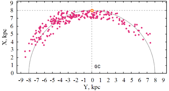
Figure 1: Distribution of the Cepheids selected for our analysis in projection onto the Galactic $XY$ plane, the circle of radius 8 kpc is shown, the position of the Sun is marked by the yellow circle, GC is the Galactic center.

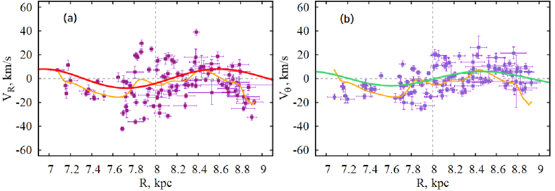
Figure 2: Radial velocities of the Cepheids $V_{R}$ (a) and their tangential velocities $V_{\theta}$ (b) as a function of distance $R$.

Table 1: The estimates of $R_{0}$ and $V_{0}$ obtained by the classic method (1)

Parameters	$r>2$ kpc	$r>2.5$ kpc	$r>3.0$ kpc	$r>3.5$ kpc	$r>4$ kpc
$N_{\star}$	117	104	94	84	75
$R_{0}\pm\varepsilon_{R_{0}},$ kpc	$7.68\pm 0.22$	$7.98\pm 0.22$	$8.24\pm 0.21$	$8.32\pm 0.18$	$8.41\pm 0.19$
$\sigma_{R_{0}},$ kpc	2.39	2.20	2.02	1.69	1.61
$V_{0}\pm\varepsilon_{V_{0}},$ km s-1	$248\pm 8$	$259\pm 8$	$265\pm 8$	$270\pm 8$	$271\pm 8$
$\sigma_{V_{0}},$ km s-1	87	82	79	71	67

Table 2: The estimates of $R_{0}$ and $V_{0}$ obtained by the method of Sofue et al. (2011) using relations (2)–(8)

Parameters	$r>2$ kpc	$r>2.5$ kpc	$r>3.0$ kpc	$r>3.5$ kpc	$r>4$ kpc
$N_{\star}$	119	105	94	86	78
$R_{0}\pm\varepsilon_{R_{0}},$ kpc	$7.44\pm 0.21$	$7.73\pm 0.21$	$7.83\pm 0.21$	$7.89\pm 0.22$	$7.97\pm 0.23$
$\sigma_{R_{0}},$ kpc	2.28	2.15	2.08	2.06	2.07
$V_{0}\pm\varepsilon_{V_{0}},$ km s-1	$239\pm 8$	$249\pm 8$	$249\pm 8$	$252\pm 8$	$252\pm 8$
$\sigma_{V_{0}},$ km s-1	82	79	76	74	74

Table 3: The estimates of $R_{0}$ and $V_{0}$ obtained by the method of Sofue et al. (2011) by additionally taking into account the influence of the spiral density wave with the following parameters: $m=4$, $\lambda=1.7$ kpc, $\chi_{\odot}=-60^{\circ},$ $f_{R}=7$ km s^-1 and $f_{\theta}=4$ km s^-1

Parameters	$r>2$ kpc	$r>2.5$ kpc	$r>3.0$ kpc	$r>3.5$ kpc	$r>4$ kpc
$N_{\star}$	122	109	97	89	80
$R_{0}\pm\varepsilon_{R_{0}},$ kpc	$7.38\pm 0.21$	$7.67\pm 0.20$	$7.78\pm 0.21$	$7.78\pm 0.22$	$7.96\pm 0.22$
$\sigma_{R_{0}},$ kpc	2.32	2.14	2.06	2.06	1.99
$V_{0}\pm\varepsilon_{V_{0}},$ km s-1	$244\pm 8$	$253\pm 8$	$252\pm 8$	$254\pm 8$	$257\pm 9$
$\sigma_{V_{0}},$ km s-1	87	82	77	78	77

DATA

The paper by Skowron et al. (2019), where the distances, ages, pulsation periods, and photometric data are given for 2431 classical Cepheids, served us as the basis for our study. The observations of these variable stars were performed within the OGLE (Optical Gravitational Lensing Experiment) program (Udalski et al. 2015). The distances to the Cepheids were calculated based on the calibration period–luminosity relations found by Wang et al. (2018) from the Cepheid light curves in the mid–infrared for eight bands. These include four bands of the WISE (Widefield Infrared Survey Explorer) catalogue (Chen et al. 2018), W1–W4: [3.35], [4.60], [11.56], and [22.09] $\mu$m, and four bands of the GLIMPSE (Spitzer Galactic Legacy Infrared Mid–Plane Survey Extraordinaire) survey (Benjamin et al. 2003): [3.6], [4.5], [5.8], and [8.0] $\mu$m. In the catalogue by Skowron et al. (2019) the extinction $A_{K_{s}}$ was calculated for each star from extinction maps. According to these authors, the Cepheid distance error in their catalogue is $\sim$5%. Skowron et al. (2019) estimated the ages using the technique of Anderson et al. (2016) by taking into account the stellar rotation period and the metallicity.

In Bobylev et al. (2021), while studying the kinematics of a large sample of classical Cepheids, we showed that the scale of Skowron et al. (2019) should be slightly extended. Therefore, in this paper the distances to the Cepheids from this catalog were increased by 10%. For our analysis we select Cepheids from the $R$ range 7–9 kpc by calculating the Galactocentric distance $R$ for them using a preliminary value of $R_{0}=8.0$ kpc.

In the method of Sofue et al. (2011) using relations (2)–(8), it is required that the stars lie in the first and fourth Galactic quadrants, i.e., in the fairly narrow longitude range $|l|<80^{\circ}$, and it is necessary to have $d\ll r$. Therefore, we apply a constraint on the coordinate x and perform our calculations with various constraints on the distance $r$. To improve the homogeneity of the sample, we take Cepheids younger than 120 Myr. Finally, there should be no high line-of-sight velocities. As a result, we use the following constraints:

$$\begin{array}[]{lll}7<R<9~{}\hbox{kpc},\\ x>0~{}\hbox{kpc},\\ \hbox{AGE}<120~{}\hbox{Myr},\\ |V_{r}|<20~{}\hbox{km s${}^{-1}$}.\end{array}$$ (13)

Under such selection conditions we obtained a sample of about 200 Cepheids with a mean age of 87 Myr. Figure 1 presents the distribution of the selected Cepheids in projection onto the Galactic $XY$ plane, where the $X$ axis is directed from the Galactic center toward the Sun and the $Y$ axis is directed along the Galactic rotation.

In Fig. 2 the radial, $V_{R}$, and tangential, $V_{\theta}$, velocities of the Cepheids are plotted against the distance $R$. Here, the Cepheids were taken under the condition $r>3$ kpc. A periodicity in both radial and tangential velocities of the Cepheids is clearly seen. The yellow lines in the figure indicate the averaged velocities (averaged by the GNUPLOT code), while the thick red and green periodic curves indicate the influence of the spiral density wave chosen by us. For this purpose, we used a four-armed ($m=4$) Galactic spiral pattern with a wavelength $\lambda=1.7$ kpc and velocity perturbation amplitudes $f_{R}$ and $f_{\theta}$ of 7 and 4 km s^-1, respectively.

RESULTS AND DISCUSSION

Tables 1–3 give the values of $R_{0}$ and $V_{0}$ obtained by three methods both without and with allowance for the influence of the spiral density wave. The data in these tables were calculated using the parameters of the solar motion relative to the local standard of rest (5).

Table 4: The estimates of $R_{0}$ and $V_{0}$ obtained by the method of Sofue et al. (2011) using relations (2)–(8) and the parameters of the solar motion relative to the local standard of rest (6)

Parameters	$r>2$ kpc	$r>2.5$ kpc	$r>3.0$ kpc	$r>3.5$ kpc	$r>4$ kpc
$N_{\star}$	107	96	89	82	75
$R_{0}\pm\varepsilon_{R_{0}},$ kpc	$8.07\pm 0.22$	$8.30\pm 0.22$	$8.30\pm 0.22$	$8.23\pm 0.22$	$8.31\pm 0.22$
$\sigma_{R_{0}},$ kpc	2.31	2.19	2.03	1.97	1.93
$V_{0}\pm\varepsilon_{V_{0}},$ km s-1	$263\pm 8$	$269\pm 8$	$265\pm 8$	$265\pm 8$	$265\pm 8$
$\sigma_{V_{0}},$ km s-1	87	84	77	75	73

Table 5: The estimates of $R_{0}$ and $V_{0}$ obtained by the method of Sofue et al. (2011) with the parameters of the solar motion relative to the local standard of rest (6) by additionally taking into account the influence of the spiral density wave with the following parameters: $m=4$, $\lambda=1.7$ kpc, $\chi_{\odot}=-60^{\circ},$ $f_{R}=7$ km s^-1 and $f_{\theta}=4$ km s^-1

Parameters	$r>2$ kpc	$r>2.5$ kpc	$r>3.0$ kpc	$r>3.5$ kpc	$r>4$ kpc
$N_{\star}$	114	102	93	84	76
$R_{0}\pm\varepsilon_{R_{0}},$ kpc	$7.80\pm 0.21$	$8.14\pm 0.20$	$8.24\pm 0.20$	$8.27\pm 0.20$	$8.35\pm 0.21$
$\sigma_{R_{0}},$ kpc	2.21	2.04	1.91	1.84	1.82
$V_{0}\pm\varepsilon_{V_{0}},$ km s-1	$258\pm 8$	$268\pm 8$	$268\pm 8$	$269\pm 8$	$269\pm 9$
$\sigma_{V_{0}},$ km s-1	89	85	80	78	78

Tables 4 and 5 give the values of $R_{0}$ and $V_{0}$ obtained by two methods both without and with allowance for the influence of the spiral density wave (just as in Tables 2 and 3) with the parameters of the solar motion relative to the local standard of rest (6).

As can be seen from Table 1, the values of $R_{0}$ and $V_{0}$ found by the classic method agree satisfactorily with the known ones, for example, those pointed out in the Introduction. However, the classic method has an important shortcoming—the line-of-sight velocities of all the Cepheids under consideration are nonzero. Therefore, the results presented in Tables 2–5 are more interesting, since they were obtained by a method free from this shortcoming. Allowance for the perturbations from the spiral density wave has a favorable effect on the estimates of $R_{0}$ and $V_{0}$. The values of $R_{0}$ and $V_{0}$ do not change fundamentally, but the dispersions $\sigma_{R_{0}}$ and the errors $\varepsilon_{R_{0}}$ decrease, though slightly. Therefore, we give preference to the parameters given in Tables 3 and 5. We are oriented to the values obtained under the constraint $r>3.0$ kpc, since there are still quite a few stars here and the errors are small.

Note that the main interest in this paper is related to the determination of $R_{0}$, while the Galactic rotation velocity at the solar distance $V_{0}$ is determined more reliably by analyzing the kinematics of large stellar samples. For example, Mróz et al. (2021) found $V_{0}=233.6\pm 2.8$ km s^-1 from the kinematics of 773 classical Cepheids with proper motions and line-of-sight velocities from the Gaia DR2 catalogue (Brown et al. 2018); Bobylev et al. (2021) obtained an estimate of $V_{0}=240\pm 3$ km s^-1 from the kinematics of $\sim$800 classical Cepheids with proper motions and line-of-sight velocities from the Gaia DR2 catalogue; Eilers et al. (2021) found $V_{0}=229.0\pm 0.2$ km s^-1 from a sample of $\sim$23 000 red giants.

As can be seen from our comparison of the data in Tables 2–4 and Tables 3–5, the results obtained depend strongly on the adopted solar velocity relative to the local standard of rest.

The following estimates were obtained from 18 Cepheids with proper motions from the Hipparcos (1997) and UCAC4 (Zacharias et al. 2012) catalogues in Bobylev (2013): $R_{0}=7.64\pm 0.32$ kpc and $V_{0}=217\pm 11$ km s^-1. In this case, the parameters from Schönrich et al. (2010) for the solar velocity (5) were used and the influence of the spiral density wave was taken into account. Thus, this result should be compared with the data in Table 3. As a result, we have good agreement between the estimates, but in this paper we used a larger number of Cepheids and, therefore, we obtained considerably smaller errors $\varepsilon_{R_{0}}$ and $\varepsilon_{V_{0}}$.

The history of the determination of the solar velocity relative to the local standard of rest is very dramatic. For example, based on data from the Hipparcos catalogue, Dehnen and Binney (1998) found $(U,V,W)_{\odot}=(10.00,5.25,7.17)$ km s^-1. If we repeat the approach of Table 4 for $r>3.0$ kpc with these velocities, then we will obtain fairly small values, $R_{0}=7.64\pm 0.21$ kpc and $V_{0}=240\pm 8$ km s^-1. The parameters (5) found by Schönrich et al. (2010) are more balanced. At present, they are widely used in kinematic studies.

The parameters of the standard solar apex $(U,V,W)_{\odot}=(10.3,15.3,7.7)$ km s^-1 were determined from a small sample of bright stars and were fixed as the solar motion with a velocity of 20 km s^-1 in the direction ($\alpha,\delta)=(18^{h},30^{\circ}$). However, these parameters are widely used by radio astronomers to maintain the continuity of the results obtained by them since the 1950s.

In Bobylev and Bajkova (2014) we showed that there is an influence of the Galactic spiral density wave on the solar velocity relative to the local standard of rest determined from young disk stars. Therefore, in our opinion, the parameters (6) take into account the solar velocity relative to the local standard of rest at the point $R=R_{0}$ more rigorously, i.e., they take into account the solar velocity perturbed by the spiral density wave at this point. Therefore, the parameters given in Tables 4 and 5 are more interesting than those in Tables 2 and 3.

In the Introduction we gave the estimates of $R_{0}$ obtained as a mean from the analysis of numerous individual determinations. Here we will note several most recent individual estimates. Leung et al. (2023) obtained an estimate of $R_{0}=8.23\pm 0.12$ kpc from the kinematics of stars in the central Galactic bar using data from the APOGEE DR17 (Apache Point Observatory Galactic Evolution Experiment, Blanton et al. 2017) and Gaia EDR3 catalogues supplemented by spectrophotometric distances. Hey et al. (2023) found $R_{0}=8108\pm 106_{\rm stat.}\pm 93_{\rm sys.}$ pc using $\sim$190 000 semiregular variables in the Galactic bulge.

It is interesting to note the paper by Gordon et al. (2023), where new absolute VLBI measurements of the radio source Sgr A* within the third International Celestial Reference Frame (ICRF 3) are presented. The observations were carried out at 52 epochs with VLBA at 24 GHz in the period 2006–2022. Based on the measured proper motion of Sgr A* in Galactic longitude, these authors estimated $V_{0}=248.0\pm 2.8$ km s^-1 (at the specified $R_{0}=8.178\pm 0.022$ kpc).

CONCLUSIONS

We obtained new estimates of the Galactocentric distance of the Sun $R_{0}$ and the Galactic rotation velocity at the solar distance $V_{0}$. They were found by a peculiar method based on the analysis of objects located near the solar circle. We used both the method in the modification of Sofue et al. (2011) and the extended method with an additional allowance for the influence of the spiral density wave. The extended method was proposed previously by Bobylev (2013) when analyzing small samples of classical Cepheids and star-forming regions.

In this paper we used a sample of classical Cepheids from the catalogue by Skowron et al. (2019), where the distances to them were determined from the period–luminosity relation with a mean random error of about 5%. The proper motions and line-of-sight velocities of the Cepheids were taken from the Gaia DR3 catalogue. We showed previously (Bobylev et al. 2021) that the Cepheid scale of Skowron et al. (2019) should be slightly extended. Therefore, in this paper the distances to the Cepheids from this catalogue were increased by 10%. For our analysis we selected $\sim$200 Cepheids with a mean age of 87 Myr located in the distance range $7<R<9$ kpc.

The values of $R_{0}$ found lie within the range [7.8–8.3] kpc, depending on the heliocentric distance of the sample stars, on the adopted solar velocity relative to the local standard of rest, and on whether or not the perturbations caused by the Galactic spiral density wave are taken into account. The dispersion of the $R_{0}$ estimates is about 2 kpc and the error of the mean is 0.2 kpc. Similarly, the values of $V_{0}$ lie within the range [240–270] km s^-1, where the dispersion of the $V_{0}$ estimates is 70–90 km s^-1 and the error of the mean is 8 km s^-1.

We deem the estimates of $R_{0}=8.24\pm 0.20$ kpc and $V_{0}=268\pm 8$ km s^-1 that were obtained from a sample of 93 Cepheids by taking into account the perturbations from the Galactic spiral density wave to be the best ones. These Cepheids are farther than 3 kpc from the Sun.

CONFLICT OF INTEREST

As author of this work, I declare that I have no conflicts of interest.

REFERENCES

1. R. Abuter, A. Amorim, M. Bauböck, et al. (GRAVITY Collab.), Astron. Astrophys. 625, L10 (2019).

2. R. Abuter, A. Amorim, M. Bauböck, et al. (GRAVITY Collab.), Astron. Astrophys. 647, A59 (2021).

3. R. I. Anderson, H. Saio, S. Ekström, C. Georgy, and G. Meynet, Astron. Astrophys. 591, A8 (2016).

4. R. A. Benjamin, E. Churchwell, B. L. Babler, T. M. Bania, D. P. Clemens, M. Cohen, J. M. Dickey, R. Indebetouw, et al., Publ. Astron. Soc. Pacif. 115, 953 (2003).

5. J. Bland-Hawthorn and O. Gerhard, Ann. Rev. Astron. Astrophys. 54, 529 (2016).

6. M. R. Blanton, M. A. Bershady, B. Abolfathi, F. D. Albareti, C. Allende Prieto, A. Almeida, J. Alonso-Garcia, F. Anders, et al., Astron. J. 154, 28 (2017).

7. V. V. Bobylev, Astron. Lett. 39, 95 (2013).

8. V. V. Bobylev and A. T. Bajkova, Mon. Not. R. Astron. Soc. 441, 142 (2014).

9. V. V. Bobylev, A. T. Bajkova, A. S. Rastorguev, and M. V. Zabolotskikh, Mon. Not. R. Astron. Soc. 502, 4377 (2021).

10. V. V. Bobylev and A. T. Bajkova, Astron. Rep. 65, 498 (2021).

11. V. V. Bobylev and A. T. Bajkova, Res. Astron. Astrophys. 23, 045001 (2023).

12. A. G. A. Brown, A. Vallenari, T. Prusti, et al. (Gaia Collab.), Astron. Astrophys. 616, 1 (2018).

13. A. G. A. Brown, A. Vallenari, T. Prusti, et al. (Gaia Collab.), Astron. Astrophys. 649, 1 (2021).

14. X. Chen, S. Wang, L. Deng, R. de Grijs, and M. Yang, Astrophys. J. Suppl. Ser., 237, 28 (2018).

15. W. Dehnen and J. J. Binney, Mon. Not. R. Astron. Soc. 298, 387 (1998).

16. A.-C. Eilers, D. W. Hogg, H.-W. Rix, and M. K. Ness, Astrophys. J. 871, 120 (2021).

17. D. Gordon, A. de Witt, and C. S. Jacobs, Astron. J. 165, 49 (2023).

18. D. R. Hey, D. Huber, B. J. Shappee, J. Bland-Hawthorn, Th. Tepper-Garcia, R. Sanderson, S. Chakrabarti, N. Saunders, et al., arXiv: 2305.19319 (2023).

19. H. S. Leavitt, Ann. Harvard College Observ. 60, 87 (1908).

20. H. S. Leavitt and E. C. Pickering, Harvard College Observ. Circ. 173, 1 (1912).

21. H. W. Leung, J. Bovy, and J. T. Mackereth, Mon. Not. R. Astron. Soc. 519, 948 (2023).

22. C. C. Lin and F. H. Shu, Astrophys. J. 140, 646 (1964).

23. B. F. Madore, Astrophys. J. 253, 575 (1982).

24. Z. Malkin, in Advancing the Physics of Cosmic Distances, Proc. IAU Symp. No. 289, 2012, Ed. R. de Grijs and G. Bono (2013).

25. P. Mróz, A. Udalski, D. M. Skowron, J. Skowron, I. Soszynski, P. Pietrukowicz, M. K. Szymanski, R. Poleski, S. Kozlowski, and K. Ulaczyk, Astrophys. J. 870, L10 (2019).

26. I. I. Nikiforov, in Order and Chaos in Stellar and Planetary Systems, Proc. Conf., August 17–24, 2003, St. Petersburg, Ed. by G. G. Byrd, K. V. Kholshevnikov, A. A. Myllari, I. I. Nikiforov and V. V. Orlov, ASP Conf. Proc. 316, 199 (2004).

27. T. Prusti, J. H. J. de Bruijne, A. G. A. Brown, et al. (Gaia Collab.), Astron. Astrophys. 595, 1 (2016).

28. M. J. Reid, Ann. Rev. Astron. Astrophys. 31, 345 (1993).

29. M. J. Reid, K. M. Menten, X. W. Zheng, A. Brunthaler, and Y. Xu, Astrophys. J. 705, 1548 (2009).

30. V. Ripepi, R. Molinaro, I. Musella, M. Marconi, S. Leccia, and L. Eyer, Astron. Astrophys. 625, 14 (2019).

31. P. L. Schechter, I.M. Avruch, J. A. R. Caldwell, and M. J. Keane, Astron. J. 104, 1930 (1992).

32. R. Schönrich, J. Binney, and W. Dehnen, Mon. Not. R. Astron. Soc. 403, 1829 (2010).

33. D. M. Skowron, J. Skowron, P. Mróz, A. Udalski, P. Pietrukowicz, I. Soszynski, M. Szymanski, R. Poleski, et al., Science (Washington, DC, U. S.) 365, 478 (2019).

34. Y. Sofue, T. Nagayama, M. Matsui, and A. Nakagawa, Publ. Astron. Soc. Jpn. 63, 867 (2011).

35. The HIPPARCOS and Tycho Catalogues, ESA SP–1200 (1997).

36. A. Udalski, M. K. Szymański, and G. Szymański, Acta Astron. 65, 1 (2015).

37. A. Vallenari, A. G. A. Brown, T. Prusti, et al. (Gaia Collab.), arXiv: 2208.0021 (2022).

38. S. Wang, X. Chen, R. de Grijs, and L. Deng, Astrophys. J. 852, 78 (2018).

39. N. Zacharias, C. T. Finch, T. M. Girard, et al., Strasbourg Catalogue No. I/322 (2012).