C^∗: A New Bounding Approach for the Moving-Target Traveling Salesman Problem

Abstract

We introduce a new bounding approach called Continuity* (C^∗) that provides optimality guarantees to the Moving-Target Traveling Salesman Problem (MT-TSP). Our approach relies on relaxing the continuity constraints on the agent’s tour. This is done by partitioning the targets’ trajectories into small sub-segments and allowing the agent to arrive at any point in one of the sub-segments and depart from any point in the same sub-segment when visiting each target. This lets us pose the bounding problem as a Generalized Traveling Salesman Problem (GTSP) in a graph where the cost of traveling an edge requires us to solve a new problem called the Shortest Feasible Travel (SFT). We also introduce C^∗-lite, which follows the same approach as C^∗, but uses simple and easy to compute lower-bounds to the SFT. We first prove that the proposed algorithms provide lower bounds to the MT-TSP. We also provide computational results to corroborate the performance of C^∗ and C^∗-lite for instances with up to 15 targets. For the special case where targets travel along lines, we compare our C^∗ variants with the SOCP based method, which is the current state-of-the-art solver for MT-TSP. While the SOCP based method performs well for instances with 5 and 10 targets, C^∗ outperforms the SOCP based method for instances with 15 targets. For the general case, on average, our approaches find feasible solutions within $\approx~{}$4$\%$ of the lower bounds for the tested instances.

I Introduction

The Traveling Salesman Problem (TSP) is one of the most important problems in optimization with several applications including unmanned vehicle planning [21, 17, 22, 28], transportation and delivery [10], monitoring and surveillance [26, 23], disaster management [4], precision agriculture [6], and search and rescue [29, 2]. Given a set of target locations (or targets) and the cost of traveling between any pair of targets, the TSP aims to find a shortest tour for a vehicle to visit each of the targets exactly once. In this paper, we consider a natural generalization of the TSP where the targets are mobile and traverse along known trajectories. The targets also have time-windows during which they must be visited. This generalization is motivated by applications in border surveillance, search and rescue, and dynamic target tracking where vehicles are required to visit or monitor a set of mobile targets. We refer to this generalization as the Moving-Target Traveling Salesman Problem, or MT-TSP for short (refer to Fig. 1). The focus of this paper is on the optimality guarantees for the MT-TSP.

The speed of any target is generally assumed [14] to be no greater than the speed of the agent since the agent is expected to visit or intercept the target at some time. If the speed of each target reduces to 0, the MT-TSP reduces to the standard TSP. Therefore, MT-TSP is a generalization of the TSP and is NP-Hard. Unlike the TSP which has been extensively studied, the current literature on MT-TSP is limited. Exact and approximation algorithms are available in the literature for some special cases of the MT-TSP where the targets are assumed to move along straight lines with constant speeds.

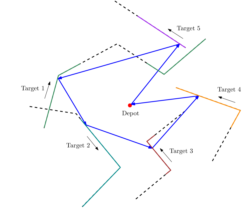
Figure 1: A feasible solution to an instance of the MT-TSP with five targets. The blue lines shows the path of the vehicle. Also, the colored solid segments for each target indicates the parts of its trajectory corresponding to its time-windows when the vehicle can visit the target.

In [3], Chalasani and Motvani propose a $(5(1+v)/3(1-v))$-approximation algorithm for the case where all the targets move in the same direction with the same speed $v$. Hammar and Nilsson [11], also present a $(1+(\epsilon/(1-v))$-approximation algorithm for the same case. They also show that the MT-TSP cannot be approximated better than a factor of $2^{\Omega(\sqrt{n})}$ by a polynomial time algorithm (unless $P=NP$), where $n$ is the number of targets. In [14], Helvig et al. develop an exact $O(n)$-time algorithm for the case when the moving targets are restricted to a single line (SL-MT-TSP). Also, for the case where most of the targets are static and at most $O(log(n)/log(log(n)))$ targets are moving out of the $n$ targets, they propose a $(2+\epsilon)$-approximation algorithm. An exact algorithm is also presented [14] for the MT-TSP with resupply where the agent must return to the depot after visiting each target; here, the targets are assumed to be far away from the depot or slow, and move along lines through the depot, towards or away from it. In [24], Stieber, and Fügenschuh formulate the MT-TSP as a second order cone program (SOCP) by relying on the key assumption that the targets travel along straight lines. Also, multiple agents are allowed, agents are not required to return to the depot, and each target has to be visited exactly once within its visibility window by one of the agents. Optimal solutions to the MT-TSP are then found for this special case.

Apart from the above methods that provide optimality guarantees to some special cases of the MT-TSP, feasible solutions can be obtained using heuristics as shown in [1, 5, 7, 8, 9, 15, 18, 25, 27]. However, these approaches do not show how far the feasible solutions are from the optimum.

A few variants of the MT-TSP and related problems have also been addressed in the literature. In [12], Hassoun et al. suggest a dynamic programming algorithm to find an optimal solution to a variant of the SL-MT-TSP where the targets move at the same speeds and may appear at different times. Masooki and Kallio in [19] address a bi-criteria variant of the MT-TSP where the number of targets vary with time and their motion is approximated using (discontinuous) step functions of time.

In this article, we consider a generalization of the MT-TSP where each target moves along piece-wise linear segments. Each target may also be associated with time windows during which the vehicle must visit the target. One way to generate feasible solutions to this problem is to sample a discrete set of times from the (planning) time horizon, and then consider the corresponding set of locations for each target; given a pair of targets and their sampled times, one can readily check for feasibility of travel and compute the travel distances between the targets. A solution can then be obtained for the MT-TSP by posing it as a generalized TSP [16] where the objective is to find an optimal TSP tour that visits exactly one (sampled) location for each target. While this approach can produce feasible solutions and upper bounds, it may not find the optimum or lower bounds for the MT-TSP. Therefore, we seek to develop methods that can provide optimality guarantees for the MT-TSP. In the special case where each target travels along a straight line, the SOCP formulation in [24] can be used to find the optimum. For the general case where each target travels along a trajectory made of piece-wise linear segments, currently, we do not know of any method in the literature that can find the optimum or provide tight lower bounds to the optimum for the MT-TSP. In this article, we develop a new approach called Continuity* (C^∗) to answer this question.

C^∗ relies on the following key ideas. First, we relax the continuity of the trajectory of the agent and allow it to be discontinuous whenever it reaches the trajectory of a target. We do this by partitioning the trajectory of each target into small sub-segments (see Fig. 2) and allow the agent to arrive at any point in a segment and depart from any point from the same segment. We then construct a graph $\mathcal{G}$ where all the nodes (sub-segments) corresponding to each target are grouped into a cluster, and any two nodes belonging to distinct clusters is connected by an edge. Next, the cost of traveling any edge is obtained by solving a Shortest Feasible Travel (SFT) problem between two sub-segments corresponding to distinct targets. Once all the costs are computed, we formulate a generalized TSP (GTSP) [16] in $\mathcal{G}$ which aims to find a tour such that exactly one node from each cluster is visited by the tour and the sum of the costs of the edges in the tour is minimum. We then show that our approach provides lower bounds to the MT-TSP. As the number of partitions or discretizations of each target’s trajectory increases, the lower bounds get better and converge to the optimum. A lower bounding solution is illustrated in Fig. 3.

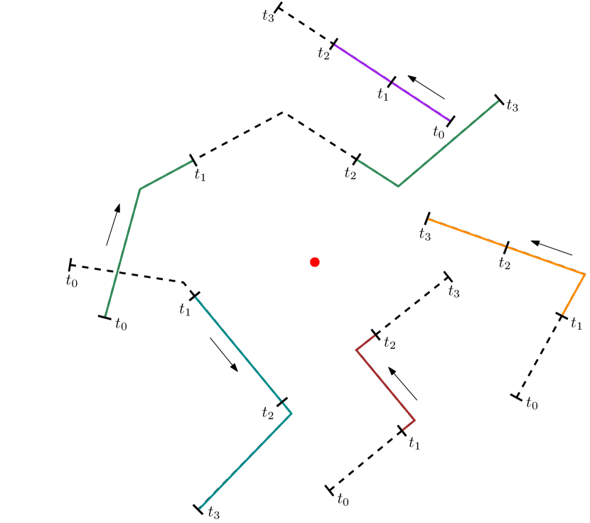
Figure 2: Partitioning of trajectories into sub-segments. For each target, only the sub-segments whose associated times lies within the target’s time-windows are considered.

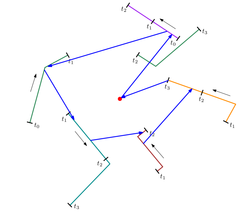
Figure 3: A feasible solution to the relaxed MT-TSP. Note the discontinuity in the agent’s tour at the sub-segments where it visits the targets.

In addition to solving the SFT problem to optimality, we also provide a simple and fast method for computing simple bounds to the cost of an edge in $\mathcal{G}$. In this way, we also develop C^∗-lite which uses the simple bounds for the optimal SFT costs in addition to C^∗ which uses optimal SFT costs. We also show how feasible solutions can be constructed from the lower bounds, though this may not be always possible if challenging time window constraints are present.

We provide computational results to corroborate the performance of C^∗ and C^∗-lite for instances with up to 15 targets. For the special case where targets travel along lines, we compare our C^∗ variants with the SOCP based method, which is the current state-of-the-art solver for MT-TSP. While the SOCP based method performs well for instances with 5 and 10 targets, C^∗ outperforms the SOCP based method for instances with 15 targets. For the general case, on average, our approaches find feasible solutions within $\approx~{}$4$\%$ of the lower bounds for the tested instances.

II Problem Definition

Let $S=\{s_{1},s_{2},\cdots,s_{n}\}$ be a set of targets. Each target $s\in S$ moves at a constant speed $v_{s}$, and follows a piecewise-linear trajectory $\pi_{s}$, where it moves along a path made of a finite set of line segments. Consider an agent that moves at a speed no greater than $v_{max}$ at any time instant. There are no other dynamic constraints placed on the motion of the agent. Let $d$ be a depot which denotes the initial location of the agent. All the targets and the agent move on a 2D plane. Also, any target $s\in S$ is associated with a set of $k$ time-windows $[t_{l,1}^{s},t_{u,1}^{s}],\cdots,[t_{l,k}^{s},t_{u,k}^{s}]$ during which times the agent can visit the target. The objective of the MT-TSP is to find a tour for the agent such that

• The agent starts and ends its tour at the depot $d$,

• The agent visits each target $s\in S$ exactly once within one of its specified time-windows $[t_{l,1}^{s},t_{u,1}^{s}],\cdots,[t_{l,k}^{s},t_{u,k}^{s}]$.

• The travel time of the agent is minimum.

III Notations and Definitions

A trajectory-point for a target $s$ is denoted by $\pi_{s}(t)$, and refers to the position occupied by the target $s$ at time $t$. The Euclidean distance between two trajectory-points $\pi_{s_{i}}(t)$ and $\pi_{s_{j}}(t^{\prime})$ or between the depot $d$ and a trajectory-point $\pi_{s}(t)$ is denoted by $D(\pi_{s_{i}}(t),\pi_{s_{j}}(t^{\prime})$) or $D(d,\pi_{s}(t))$ respectively. A trajectory-interval for a target $s$ is denoted by $\pi_{s}[t_{p},t_{q}]$, and refers to the set of all the positions occupied by $s$ over the time interval $[t_{p},t_{q}]$, where $t_{q}\geq t_{p}$. Suppose the time interval $[t_{r},t_{s}]$ lies within another time interval $[t_{p},t_{q}]$ ($i.e.$ $[t_{r},t_{s}]\subseteq[t_{p},t_{q}]$). Then, $\pi_{s}[t_{r},t_{s}]$ is a trajectory-sub-interval that lies within the trajectory-interval $\pi_{s}[t_{p},t_{q}]$.

A travel from $\pi_{s_{i}}(t)$ to $\pi_{s_{j}}(t^{\prime})$ denotes the event where the agent departs from $\pi_{s_{i}}(t)$ at time $t$, and arrives at $\pi_{s_{j}}(t^{\prime})$ at time $t^{\prime}$. This is the same as saying the agent departs from $s_{i}$ at time $t$ and arrives at $s_{j}$ at time $t^{\prime}$. For travel from the depot $d$ to $\pi_{s}(t)$, the agent departs from $d$ at time $t_{d}=0$, and for travel from $\pi_{s}(t)$ to $d$, the agent arrives at $d$ at some time $t_{d}\geq t$.

A travel is feasible if the agent can complete it without exceeding its maximum speed $v_{max}$. Clearly, feasible travel requires the arrival time to be greater than or equal to the departure time. Let $T$ denote the time-horizon. We say a feasible travel exists from $\pi_{s_{i}}(t_{p})$ (or $d$) to $\pi_{s_{j}}$, if there exists some $t\in[t_{p},T]$ such that travel from $\pi_{s_{i}}(t_{p})$ (or $d$) to $\pi_{s_{j}}(t)$ is feasible. Similarly, we say a feasible travel exists from $\pi_{s_{i}}$ to $\pi_{s_{j}}(t_{p})$ if there exists some time $t\in[0,T]$ such that the travel from $\pi_{s_{i}}(t)$ to $\pi_{s_{j}}(t_{p})$ is feasible. Arriving at the depot from a trajectory-point is always feasible since the depot has no fixed time of arrival. Finally, we say a feasible travel exists from some trajectory-interval $\pi_{s_{i}}[t_{p},t_{q}]$ to another trajectory-interval $\pi_{s_{j}}[t_{r},t_{s}]$, if there exists some $t\in[t_{p},t_{q}]$ and some $t^{\prime}\in[t_{r},t_{s}]$ such that the travel from $\pi_{s_{i}}(t)$ to $\pi_{s_{j}}(t^{\prime})$ is feasible. Similarly, if the travel from $d$ to $\pi_{s}(t)$ where $t\in[t_{p},t_{q}]$ is feasible, then there exists a feasible travel from $d$ to $\pi_{s}[t_{p},t_{q}]$.

Now, we define the following optimization problems between any two targets which we need to solve as part of our approach to the MT-TSP:

• Earliest Feasible Arrival Time (EFAT) Problem:

  • $\min t$ such that $t\in[t_{p},T]$ and the travel from $\pi_{s_{i}}(t_{p})$ to $\pi_{s_{j}}(t)$ is feasible.

  • $\min t$ such that $t\in[0,T]$ and the travel from $d$ to $\pi_{s}(t)$ is feasible.

  The optimal times (also referred to as EFATs) to the above problems are denoted as $e(t_{p})$ and $e(t_{d})$ respectively. Also, $\pi_{s_{j}}(e(t_{p}))$ and $\pi_{s}(e(t_{d}))$ denotes the earliest feasible arrivals (EFAs) from $\pi_{s_{i}}(t_{p})$ to $\pi_{s_{j}}$ and $d$ to $\pi_{s}$ respectively.

• Latest Feasible Departure Time (LFDT) Problem: $\max t$ such that $t\in[0,T]$ and the travel from $\pi_{s_{i}}(t)$ to $\pi_{s_{j}}(t_{p})$ is feasible. Let $l(t_{p})$ denote the optimal time (LFDT) to this problem, and let $\pi_{s_{i}}(l(t_{p}))$ denote the latest feasible departure (LFD) from $\pi_{s_{i}}$ to $\pi_{s_{j}}(t_{p})$.

• SFT problems:

  • SFT from $\pi_{s_{i}}[t_{p},t_{q}]$ to $\pi_{s_{j}}[t_{r},t_{s}]$: $\min_{t,t^{\prime}}\ {(t^{\prime}-t)}$ where $t\in[t_{p},t_{q}],\ t^{\prime}\in[t_{r},t_{s}]$, and travel from $\pi_{s_{i}}(t)$ to $\pi_{s_{j}}(t^{\prime})$ is feasible.

  • SFT from $d$ to $\pi_{s}[t_{p},t_{q}]$: $\min{t}$ where $t\in[t_{p},t_{q}]$, and travel from $d$ to $\pi_{s}(t)$ is feasible.

  • SFT from $\pi_{s}[t_{p},t_{q}]$ to $d$: $\min_{t}\ {D(d,\pi_{s}(t)})/v_{max}$ where $t\in[t_{p},t_{q}]$.

  • SFT from $\pi_{s_{i}}(t_{p})$ to $\pi_{s_{j}}[t_{r},t_{s}]$: $\min_{t}\ (t-t_{p})$ where $t\in[t_{r},t_{s}]$, and travel from $\pi_{s_{i}}(t_{p})$ to $\pi_{s_{j}}(t)$ is feasible.

  • SFT from $\pi_{s_{i}}(t_{p})$ to $\pi_{s_{j}}$: $\min_{t}\ (t-t_{p})$ where $t\in[0,T]$, and travel from $\pi_{s_{i}}(t_{p})$ to $\pi_{s_{j}}(t)$ is feasible.

  • SFT from $d$ to $\pi_{s}$: $\min t$ where $t\in[0,T]$, and travel from $d$ to $\pi_{s}(t)$ is feasible.

  • SFT from $\pi_{s_{i}}$ to $\pi_{s_{j}}(t_{p})$: $\min_{t}\ (t_{p}-t)$ where $t\in[0,T]$, and travel from $\pi_{s_{i}}(t)$ to $\pi_{s_{j}}(t_{p})$ is feasible.

  Clearly, $t:=e(t_{p})$ is the solution to the third to last problem, $t:=e(t_{d})$ is the solution to the second to last problem, and $t:=l(t_{p})$ is the solution to the last problem.

IV C^∗ Algorithm

IV-A Overview

The main idea behind C^∗ is to relax the MT-TSP by allowing discontinuities in the agent’s tour. The relaxed problem can then be formulated as an GTSP on a newly constructed graph $\mathcal{G}$, which when solved to optimality, gives a lower-bound to the MT-TSP.

We begin by discretizing the time-horizon $T$ into $m$ intervals $[t_{0},t_{1}],[t_{1},t_{2}],\cdots,[t_{m-1},t_{m}]$. Without loss of generality, for each target, assume that any time in $\{t_{0},t_{1},\cdots,t_{m}\}$ coincides with one of the endpoints of the time-windows specified for the target (refer to the problem statement). For each target $s\in S$, if $[t_{k},t_{k+1}]$ for $k=0,\cdots,m-1$ lies within one of the time-windows associated with $s$, we add the trajectory-interval $\pi_{s}[t_{k},t_{k+1}]$ to a cluster $C_{s}$. This allows us to construct the graph $\mathcal{G}$ with the nodes consisting of the depot (depot-node), and all the trajectory-intervals within the clusters (trajectory-nodes). Directed edges are added between trajectory-nodes of different clusters, from the depot-node to trajectory-nodes, and from trajectory-nodes to the depot-node. The cost of the edges between any two nodes in $\mathcal{G}$ are obtained by solving the SFT problems. This approach allows the agent to arrive at any point within a trajectory-interval, and depart from any point within the same trajectory-interval when visiting each target. More details on finding the SFT will be given in section IV-B. The relaxed problem can now be formulated as an GTSP on $\mathcal{G}$, with $C_{s_{i}}$ for $i=1,\cdots,n$ being the clusters. The optimal solution to the GTSP provides a lower-bound on the optimal solution to the MT-TSP. As the number of intervals that discretizes $T$ approaches infinity, the lower-bound converges to the optimal solution to the MT-TSP. All of this will be proved in section IV-D.

IV-B Algorithms for solving the SFT problems

In this section, we present approaches to solve the SFT problem. We consider three cases: Finding the SFT between two trajectory-intervals, finding the SFT from the depot to some trajectory-interval, and finding the SFT from some trajectory-interval back to the depot.

Consider the first case. Let $\pi_{s_{i}}[t_{p},t_{q}]$ be a trajectory-interval for some target $s_{i}$, and let $\pi_{s_{j}}[t_{r},t_{s}]$ be a trajectory-interval for another target $s_{j}$. The objective is to find the SFT from $\pi_{s_{i}}[t_{p},t_{q}]$ to $\pi_{s_{j}}[t_{r},t_{s}]$. The procedure to do this can be broken into five main steps; feasibility check, special case check, search space reduction, sampling, and finally, optimal travel search.

The main intuition behind these steps is to decompose the original problem of finding the SFT between two piecewise-linear trajectory-intervals, into easier sub-problems of finding the SFTs between a number of linear trajectory-sub-interval pairs, if an obvious solution cannot be found early on. Each sub-problem can be solved by minimizing a corresponding function which finds the difference $e(t)-t$ for some $t$ associated with the start linear trajectory-sub-interval.

IV-B1 Feasibility Check

The first step is to check if travel from $\pi_{s_{i}}[t_{p},t_{q}]$ to $\pi_{s_{j}}[t_{r},t_{s}]$ is feasible. Note that this travel is feasible if and only if travel from $\pi_{s_{i}}(t_{p})$ to $\pi_{s_{j}}(t_{s})$ is feasible. We will prove this in section IV-D. If not feasible, the search is terminated and the SFT cost is set to a large value since one does not exist in this case. If feasible, proceed to the next step.

IV-B2 Special Case Check

The second step is to check if travel from $\pi_{s_{i}}(t_{q})$ to $\pi_{s_{j}}(t_{r})$ is feasible. If feasible, clearly this will be the SFT from $\pi_{s_{i}}[t_{p},t_{q}]$ to $\pi_{s_{j}}[t_{r},t_{s}]$, and the cost of SFT will be $t_{r}-t_{q}$. If not feasible, proceed to the next step.

IV-B3 Search Space Reduction

The third step is to reduce the search space by discarding parts of $\pi_{s_{i}}[t_{p},t_{q}]$ and $\pi_{s_{j}}[t_{r},t_{s}]$ that does not allow the SFT. First find $e(t_{p})$ and $e(t_{q})$ as shown in Fig. 4 (a). Note that if $e(t_{q})\notin[0,T]$, use $T$ in place of $e(t_{q})$. Next, find the intersection $[t_{b_{i}},t_{b_{f}}]$ between $[e(t_{p}),e(t_{q})]$ and $[t_{r},t_{s}]$ (i.e. $[t_{b_{i}},t_{b_{f}}]=[e(t_{p}),e(t_{q})]\cap[t_{r},t_{s}]$) as shown in Fig. 4 (b). In section IV-D, we will prove that this intersection must always exist if the feasibility check is satisfied and the special case check is not satisfied. Given $[t_{b_{i}},t_{b_{f}}]\subseteq[t_{r},t_{s}]$, now find $[t_{a_{i}},t_{a_{f}}]\subseteq[t_{p},t_{q}]$ where $t_{a_{i}}=l(t_{b_{i}})$ and $t_{a_{f}}=l(t_{b_{f}})$. This is also shown in Fig. 4 (b). Note that the SFT from $\pi_{s_{i}}[t_{p},t_{q}]$ to $\pi_{s_{j}}[t_{r},t_{s}]$ will now be the same as the SFT from $\pi_{s_{i}}[t_{a_{i}},t_{a_{f}}]$ to $\pi_{s_{j}}[t_{b_{i}},t_{b_{f}}]$. This will be proved in section IV-D. As a part of this proof, we show that $[t_{a_{i}},t_{a_{f}}]\subseteq[t_{p},t_{q}]$ is indeed true. Once the search space is reduced, proceed to the next step.

IV-B4 Sampling

The fourth step is to sample the time intervals $[t_{a_{i}},t_{a_{f}}]$ and $[t_{b_{i}},t_{b_{f}}]$ into sub-intervals. To do this, first find all the critical times for target $s_{i}$ where it changes direction within $(t_{a_{i}},t_{a_{f}})$, and add these times along with $t_{a_{i}}$ and $t_{a_{f}}$ to an empty set CritStart. Similarly, find all the critical times for target $s_{j}$ where it changes direction within $(t_{b_{i}},t_{b_{f}})$, and add these times along with $t_{b_{i}}$ and $t_{b_{f}}$ to an empty set CritDest. Next, find the EFAT for all the critical times for $s_{i}$, and add it to CritDest. Note that they will lie within $(t_{b_{i}},t_{b_{f}})$. Similarly, find the LFDT for all the critical times for $s_{j}$, and add it to CritStart. Once again, note they will lie within $(t_{a_{i}},t_{a_{f}})$. Next, sort every times within CritStart and CritDest from earliest to latest, and add it to lists CritStartSort, and CritDestSort, respectively. Finally, sample $[t_{a_{i}},t_{a_{f}}]$ and $[t_{b_{i}},t_{b_{f}}]$ into sub-intervals, with adjacent times in CritStartSort and CritDestSort respectively as their endpoints. The sampling step is illustrated in Fig. 4 (c). Note how CritStartSort and CritDestSort have the same length. This is because two different times cannot share the same EFAT or LFDT. We will prove this in section IV-D. Also, note how the trajectory-sub-intervals for all the sub-intervals obtained from $[t_{a_{i}},t_{a_{f}}]$ and $[t_{b_{i}},t_{b_{f}}]$ are linear segments. Once the sampling step is complete, the SFT from $\pi_{s_{i}}[t_{a_{i}},t_{a_{f}}]$ to $\pi_{s_{j}}[t_{b_{i}},t_{b_{f}}]$ can be obtained by following the next step.

Remark 1.

After sampling, let $[t_{c},t_{d}]$ be one of the sub-intervals within $[t_{a_{i}},t_{a_{f}}]$ and let $[t_{e},t_{f}]$ be the corresponding sub-interval within $[t_{b_{i}},t_{b_{f}}]$ with the same index as $[t_{c},t_{d}]$. Clearly, either $t_{e}=e(t_{c})$ or $t_{c}=l(t_{e})$ and also, either $t_{f}=e(t_{d})$ or $t_{d}=l(t_{f})$. Then, $[t_{e},t_{f}]$ is the collection of EFATs for all times in $[t_{c},t_{d}]$. Consequently, for some $t_{a}\in[t_{c},t_{d}]$, the SFT from $\pi_{s_{i}}(t_{a})$ to $\pi_{s_{j}}[t_{b_{i}},t_{b_{f}}]$ must end at $\pi_{s_{j}}(t_{b})$ where $t_{b}=e(t_{a})\in[t_{e},t_{f}]$. All of this will be proved in section IV-D.

IV-B5 Optimal Travel Search

The fifth step is to find the SFT from each trajectory-sub-interval in $\pi_{s_{i}}[t_{a_{i}},t_{a_{f}}]$ to its corresponding trajectory-sub-interval in $\pi_{s_{j}}[t_{b_{i}},t_{b_{f}}]$, and choose the SFT with the minimum cost. Let $[t_{c},t_{d}]$ be one of the sub-intervals within $[t_{a_{i}},t_{a_{f}}]$ and let $[t_{e},t_{f}]$ be its corresponding sub-interval within $[t_{b_{i}},t_{b_{f}}]$. The SFT from $\pi_{s_{i}}[t_{c},t_{d}]$ to $\pi_{s_{j}}[t_{e},t_{f}]$ can then be found by formulating a function $f$ which for some time $t\in[t_{c},t_{d}]$, gives $e(t)-t$ (recall $e(t)\in[t_{e},t_{f}]$), and by finding $t:=t^{*}$ that minimizes $f$. The function minimum $f^{*}$, as well as $t^{*}$ can be obtained by comparing $f$ evaluated at $t_{c}$, $t_{d}$, and all the stationary points of $f$ within $[t_{c},t_{d}]$. Since $\pi_{s_{i}}[t_{c},t_{d}]$ is a linear segment and $\pi_{s_{j}}[t_{e},t_{f}]$ is also a linear segment, the stationary points of $f$ can be obtained by finding the roots to a quadratic polynomial, and choosing the roots that lie within $[t_{c},t_{d}]$. More details on this will be given in the section  VII along with details on finding the EFAT and LFDT. The SFT from $\pi_{s_{i}}[t_{c},t_{d}]$ to $\pi_{s_{j}}[t_{e},t_{f}]$ will then be from $\pi_{s_{i}}(t^{*})$ to $\pi_{s_{j}}(e(t^{*}))$, and the cost of the SFT will be $f^{*}=e(t^{*})-t^{*}$.

This concludes the first case of finding the SFT between two trajectory-intervals. Now, consider the second case. The objective is to find the SFT from the depot $d$, to some trajectory-interval $\pi_{s}[t_{p},t_{q}]$. The steps here are similar to the first case. The first step is to check if travel from $d$ to $\pi_{s}[t_{p},t_{q}]$ is feasible, by checking if travel from $d$ to $\pi_{s}(t_{q})$ is feasible. If not true, the search will be terminated and a large value is assigned as the SFT cost. If true, the next step is to check if travel from $d$ to $\pi_{s}(t_{p})$ is feasible. If true, clearly this will be the SFT from $d$ to $\pi_{s}[t_{p},t_{q}]$ and the associated cost will be $t_{p}$. If not true, the SFT from $d$ to $\pi_{s}[t_{p},t_{q}]$ will be from $d$ to $\pi_{s}(e(t_{d}))$ and will have cost $e(t_{d})$. The proofs for this will be provided in section IV-D.

Finally, consider the third case. The objective is to find the SFT from some trajectory-interval $\pi_{s}[t_{p},t_{q}]$, back to the depot $d$. Let $\pi_{s}(t^{*})$, where $t^{*}\in[t_{p},t_{q}]$, be the trajectory-point in $\pi_{s}[t_{p},t_{q}]$ which is at the closest distance from $d$. Then travel from $\pi_{s}(t^{*})$ to $d$ at the maximum agent speed $v_{max}$ is the SFT from $\pi_{s}[t_{p},t_{q}]$ to $d$ since the time taken by the agent to reach $d$ from $\pi_{s}[t_{p},t_{q}]$ is minimized when the agent follows the minimum distance path at its maximum speed. The associated SFT cost will be $D(d,\pi_{s}(t^{*}))/v_{max}$.

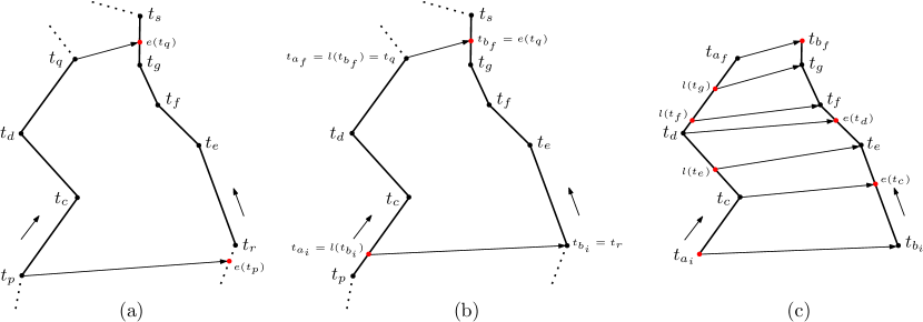
Figure 4: (a) $e(t_{p})$ and $e(t_{q})$ are found. (b) The intersection $[t_{b_{i}},t_{b_{f}}]=[e(t_{p}),e(t_{q})]\cap[t_{r},t_{s}]$ is found. Here, $[t_{b_{i}},t_{b_{f}}]=[t_{r},e(t_{q})]$. Also, $[t_{a_{i}},t_{a_{f}}]=[l(t_{b_{i}}),l(t_{b_{f}})]$ is found. Note how $t_{a_{f}}=l(e(t_{q}))=t_{q}$. This is because, $l(e(t))=t$ and $e(l(t))=t$ for some $t$. We will prove this in section IV-D. (c) CritStartSort is $[t_{a_{i}},t_{c},l(t_{e}),t_{d},l(t_{f}),l(t_{g}),t_{a_{f}}]$ and CritDestSort is $[t_{b_{i}},e(t_{c}),t_{e},e(t_{d}),t_{f},t_{g},t_{b_{f}}]$. Next, $[t_{a_{i}},t_{a_{f}}]$ is sampled into sub-intervals $[t_{a_{i}},t_{c}],[t_{c},l(t_{e})],\cdots,[l(t_{g}),t_{a_{f}}]$, and $[t_{b_{i}},t_{b_{f}}]$ is sampled into sub-intervals $[t_{b_{i}},e(t_{c})],[e(t_{c}),t_{e}],\cdots,[t_{g},t_{b_{f}}]$. We say each sub-interval in $[t_{b_{i}},t_{b_{f}}]$ corresponds to the sub-interval with the same index in $[t_{a_{i}},t_{a_{f}}]$ after sampling. For e.g., $[e(t_{c}),t_{e}]$ corresponds to $[t_{c},l(t_{e})]$ since they are both the 2nd sub-interval in $[t_{b_{i}},t_{b_{f}}]$ and $[t_{a_{i}},t_{a_{f}}]$ respectively. To find the optimal travel, compare the SFT from $\pi_{s_{i}}[t_{a_{i}},t_{c}]$ to $\pi_{s_{j}}[t_{b_{i}},e(t_{c})]$, $\pi_{s_{i}}[t_{c},l(t_{e})]$ to $\pi_{s_{j}}[e(t_{c}),t_{e}]$, and so on and choose the SFT with minimum cost.

IV-C C^∗-lite: A simplified C^∗

In this section, we simplify C^∗ to obtain C^∗-lite. The steps for C^∗-lite are the same as the steps for C^∗, except for one modification. All the SFTs in C^∗ are replaced with simple lower-bounds to the SFTs in C^∗-lite. For the remainder of this section, we explain these simple lower-bounds. Again, we consider three cases.

First, consider the first case where the objective is to find a lower-bound on the SFT between two trajectory-intervals $\pi_{s_{i}}[t_{p},t_{q}]$ and $\pi_{s_{j}}[t_{r},t_{s}]$. If a SFT exists, then travel between the two trajectory-intervals must be feasible. Hence, the first step is to repeat the procedure from feasibility check in section IV-B. The next step is to check whether $t_{r}<t_{q}$. If true, set the cost of travel from $\pi_{s_{i}}[t_{p},t_{q}]$ to $\pi_{s_{j}}[t_{r},t_{s}]$ to $0$. The travel from $\pi_{s_{i}}(t_{q})$ to $\pi_{s_{j}}(t_{r})$ is clearly infeasible in this case. However, $0$ cost will be a lower-bound on the SFT cost. If not true, set the cost of travel from $\pi_{s_{i}}[t_{p},t_{q}]$ to $\pi_{s_{j}}[t_{r},t_{s}]$ to $t_{r}-t_{q}$. This is similar to the special case check in section IV-B, except that the travel from $\pi_{s_{i}}(t_{q})$ to $\pi_{s_{j}}(t_{r})$ is not required to be feasible here. If feasible, the cost of travel becomes equal to the SFT cost. However if not, the cost of travel still remains a lower-bound on the SFT cost.

Now, consider the second case where the objective is to find a lower-bound on the SFT from the depot $d$, to some trajectory-interval $\pi_{s}[t_{p},t_{q}]$. Since SFT requires this travel to be feasible, once again check for feasibility by checking if the travel from $d$ to $\pi_{s}(t_{q})$ is feasible. If feasible, set the cost of travel to $t_{p}$. If travel from $d$ to $\pi_{s}(t_{p})$ is feasible, this cost becomes equal to the SFT cost as seen in section IV-B. However, if not feasible, this cost still clearly remains a lower-bound on the SFT cost. If travel from $d$ to $\pi_{s}[t_{p},t_{q}]$ is not feasible, set the cost of travel to a large value.

Finally, consider the third case where the objective is to find a lower-bound on the SFT from some trajectory-interval $\pi_{s}[t_{p},t_{q}]$, back to the depot $d$. In this case, we set the lower-bound cost to be equal to the SFT cost.

IV-D Validity of C^∗ and the SFT Algorithms

In this section, we will show that C^∗ provides a lower-bound to the MT-TSP. Then, we will verify that correctness of the approach to solve the SFT problems.

Theorem 1.

The optimal solution to the relaxed MT-TSP obtained in C^∗ provides a lower-bound on the optimal solution to the MT-TSP.

Proof.

Consider the optimal tour to the MT-TSP where the agent travels from $d$ to $\pi_{s_{1}^{\prime}}(t_{1}^{\prime})$, then travels from $\pi_{s_{i}^{\prime}}(t_{i}^{\prime})$ to $\pi_{s_{i+1}^{\prime}}(t_{i+1}^{\prime})$ for $i=1,\cdots,n-1$ and finally travels from $\pi_{s_{n}}^{\prime}(t_{n}^{\prime})$ to $d$ at speed $v_{max}$. Note that the sequence corresponding to the optimal tour is then ${s_{1}^{\prime},\cdots,s_{n}^{\prime}}$. Let the time at which the agent returns to $d$ be $t_{tour}$. Then, the time taken by the agent to complete the tour is $t_{tour}=(t_{1}^{\prime}-0)+\sum_{i=1}^{n-1}(t^{\prime}_{i+1}-t^{\prime}_{i})+(t_{tour}-t_{n}^{\prime})$. Note that $t_{i}^{\prime}$ lies within some interval $[t^{-}_{i},t^{+}_{i}]$ for $i=1,\cdots,n$. Let the cost of the SFT from $d$ to $\pi_{s_{1}^{\prime}}[t^{-}_{1},t^{+}_{1}]$ be $c_{0}$, the cost of SFT from $\pi_{s_{i}^{\prime}}[t^{-}_{i},t^{+}_{i}]$ to $\pi_{s^{\prime}_{i+1}}[t^{-}_{i+1},t^{+}_{i+1}]$ be $c_{i}$ for $i=1,\cdots,n-1$ and the cost of the SFT from $\pi_{s_{n}^{\prime}}[t^{-}_{n},t^{+}_{n}]$ to $d$ be $c_{n}$. Clearly, $c_{0}\leq(t^{\prime}_{1}-t_{0})$, $c_{i}\leq(t_{i+1}^{\prime}-t_{i}^{\prime})$ for $i=1,\cdots,n-1$ and $c_{n}\leq(t_{tour}-t^{\prime}_{n})$. Now, consider a feasible solution to the relaxed MT-TSP where a cycle starts at $d$, visits $\pi_{s_{i}^{\prime}}[t^{-}_{i},t^{+}_{i}]$ for $i=1,\cdots,n$ in that order, and ends at $d$. Then the cost of this cycle is $\sum_{i=0}^{n}c_{i}\leq t_{tour}$. Hence, the optimal solution to the relaxed MT-TSP must have a cost less than or equal to $\sum_{i=0}^{n}c_{i}$, providing a lower-bound on the optimal solution to the MT-TSP. ∎

Remark 2.

As the number of discretizations of $T$ into time intervals tend to infinity, the size of each interval and that of the discontinuities also tend to zero. Since for any discretization of $T$, C^∗ provides a lower bound, the optimal cost of the relaxed MT-TSP converges asymptotically to the optimal cost to the MT-TSP as the number of discretizations of $T$ approaches infinity.

Now, consider the SFT between two trajectory-intervals. Suppose an agent with maximum speed $v_{max}$ departs from some target $s_{i}$ and heads towards another target $s_{j}$. Let $\pi_{s_{i}}(t_{p})$ and $\pi_{s_{i}}(t_{q})$ be two trajectory-points and let $\pi_{s_{j}}(e(t_{p}))$ and $\pi_{s_{j}}(e(t_{q}))$ be the EFAs from $\pi_{s_{i}}(t_{p})$ and $\pi_{s_{i}}(t_{q})$ to $\pi_{s_{j}}$. Similarly, let $\pi_{s_{j}}(t_{r})$ and $\pi_{s_{j}}(t_{s})$ be two trajectory-points and let $\pi_{s_{i}}(l(t_{r}))$ and $\pi_{s_{i}}(l(t_{s}))$ be the LFDs from $\pi_{s_{i}}$ to $\pi_{s_{j}}(t_{r})$ and $\pi_{s_{j}}(t_{s})$. Assume that the targets follow time-continuous trajectories with some generic shape at a constant speed and that the maximum agent speed is greater than the fastest target speed. Then the following is true.

Lemma 1.

If the agent can travel feasibly from $\pi_{s_{i}}(t_{p})$ to $\pi_{s_{j}}(t_{r})$ by moving at some speed $v$, then for any $t>t_{r}$, the agent can travel feasibly directly from $\pi_{s_{i}}(t_{p})$ to $\pi_{s_{j}}(t)$ by moving at some speed $v^{\prime}$. If $t_{r}>t_{p}$ and $v>v_{s_{j}}$, then $v^{\prime}<v$.

Proof.

The agent can travel feasibly from $\pi_{s_{i}}(t_{p})$ to $\pi_{s_{j}}(t)$ by first traveling feasibly from $\pi_{s_{i}}(t_{p})$ to $\pi_{s_{j}}(t_{r})$ by moving at speed $v$ and then following the target $s_{j}$ from time $t_{r}$ to time $t$ by moving at speed $v_{s_{j}}$. Let $L$ be the length of the path followed by $s_{j}$ from time $t_{r}$ to time $t$. Also, let $d_{1}=D(\pi_{s_{i}}(t_{p}),\pi_{s_{j}}(t_{r}))$ and $d_{2}=D(\pi_{s_{i}}(t_{p}),\pi_{s_{j}}(t))$. Note that since $d_{2}\leq d_{1}+L$, the agent can also travel feasibly directly from $\pi_{s_{i}}(t_{p})$ to $\pi_{s_{j}}(t)$ by moving at some speed $v^{\prime}$. Now assume $t_{r}>t_{p}$ and $v>v_{s_{j}}$. Then clearly, $d_{1}>0$. If $d_{2}=0$, then $v^{\prime}=0\leq v_{s_{j}}<v$. However if $d_{2}>0$, we consider two cases. First case is when $v_{s_{j}}=0$. In this case $L=0$ and therefore, $d_{2}=d_{1}$. Since $t-t_{p}>t_{r}-t_{p}$, clearly $v^{\prime}<v$. Second case is when $v_{s_{j}}>0$. In this case, $t-t_{p}=(t-t_{r})+(t_{r}-t_{p})\implies d_{2}/v^{\prime}=L/v_{s_{j}}+d_{1}/v>L/v+d_{1}/v\implies v^{\prime}<vK$ where $K=d_{2}/(L+d_{1})$. Since $0<K\leq 1$, we see that $v^{\prime}<v$. ∎

Lemma 2.

Suppose $\pi_{s_{i}}$ and $\pi_{s_{j}}$ does not intersect at time $t_{p}$ (i.e. $\pi_{s_{i}}(t_{p})\neq\pi_{s_{j}}(t_{p})$). Then travel from $\pi_{s_{i}}(t_{p})$ to $\pi_{s_{j}}(e(t_{p}))$ requires the maximum agent speed $v_{max}$. Also, if the agent travels feasibly from $\pi_{s_{i}}(t_{p})$ to $\pi_{s_{j}}(t_{r})$ by moving at its maximum speed $v_{max}$, then $t_{r}=e(t_{p})$.

Proof.

Let $\pi_{s_{i}}(t_{p})\neq\pi_{s_{j}}(t_{p})$. Then clearly, $e(t_{p})>t_{p}$. Let $v$ be the agent speed required to travel from $\pi_{s_{i}}(t_{p})$ to $\pi_{s_{j}}(e(t_{p}))$. Note that $v\leq v_{max}$ is required since the travel is feasible. If $s_{j}$ is stationary, clearly $v=v_{max}$. In the general case where $s_{j}$ moves, if $v<v_{max}$, then by moving at speed $v=v_{max}$ instead, the agent can depart from $s_{i}$ at time $t_{p}$, and arrive at the trajectory-point $\pi_{s_{j}}(e(t_{p}))$ at some time $t$ before target $s_{j}$ reaches this point, and then visit $s_{j}$ by traversing the path it follows from time $t$ to time $e(t_{p})$, in the reverse direction. This way, the agent visits $s_{j}$ at some time earlier than $e(t_{p})$ which contradicts the fact that $e(t_{p})$ is the EFAT. Hence, $v=v_{max}$. Now, let $v(t)$ represent the agent speed required to travel from $\pi_{s_{i}}(t_{p})$ to $\pi_{s_{j}}(t)$ for some time $t$. Assume that the agent travels feasibly from $\pi_{s_{i}}(t_{p})$ to $\pi_{s_{j}}(t_{r})$ by moving at speed $v_{max}$. Since the travel is feasible, $t_{r}\geq e(t_{p})$. If $t_{r}>e(t_{p})$, then since $e(t_{p})>t_{p}$ and $v(e(t_{p}))=v_{max}>v_{s_{j}}$, using lemma 1, $v(t_{r})<v_{max}$ which contradicts our assumption. Hence, $t_{r}=e(t_{p})$. ∎

Remark 3.

If $\pi_{s_{i}}$ and $\pi_{s_{j}}$ intersects at time $t_{p}$ (i.e. $\pi_{s_{i}}(t_{p})=\pi_{s_{j}}(t_{p})$), then $e(t_{p})=t_{p}$ and the agent speed required to travel from $\pi_{s_{i}}(t_{p})$ to $\pi_{s_{j}}(e(t_{p}))$ is not unique. Hence, an agent speed of $v_{max}$ is not necessary, but still sufficient in this special case.

Lemma 3.

If the agent can travel feasibly from $\pi_{s_{i}}(t_{p})$ to $\pi_{s_{j}}(t_{r})$ by moving at some speed $v$, then for any $0\leq t<t_{p}$, the agent can travel feasibly directly from $\pi_{s_{i}}(t)$ to $\pi_{s_{j}}(t_{r})$ by moving at some speed $v^{\prime}$. If $t_{r}>t_{p}$ and $v>v_{s_{i}}$, then $v^{\prime}<v$.

Proof.

The agent can travel feasibly from $\pi_{s_{i}}(t)$ to $\pi_{s_{j}}(t_{r})$ by first following the target $s_{i}$ from time $t$ to time $t_{p}$ by moving at speed $v_{s_{i}}$ and then traveling feasibly from $\pi_{s_{i}}(t_{p})$ to $\pi_{s_{j}}(t_{r})$ by moving at speed $v$. Let $L$ be the length of the path followed by $s_{i}$ from time $t$ to time $t_{p}$. Also, let $d_{1}=D(\pi_{s_{i}}(t_{p}),\pi_{s_{j}}(t_{r}))$ and $d_{2}=D(\pi_{s_{i}}(t),\pi_{s_{j}}(t_{r}))$. Note that since $d_{2}\leq d_{1}+L$, the agent can also travel feasibly directly from $\pi_{s_{i}}(t)$ to $\pi_{s_{j}}(t_{r})$ by moving at some speed $v^{\prime}$. Now assume $t_{r}>t_{p}$ and $v>v_{s_{i}}$. Then clearly, $d_{1}>0$. If $d_{2}=0$, then $v^{\prime}=0\leq v_{s_{i}}<v$. However if $d_{2}>0$, we consider two cases. First case is when $v_{s_{i}}=0$. In this case $L=0$ and therefore, $d_{2}=d_{1}$. Since $t_{r}-t>t_{r}-t_{p}$, clearly $v^{\prime}<v$. Second case is when $v_{s_{i}}>0$. In this case, $t_{r}-t=(t_{r}-t_{p})+(t_{p}-t)\implies d_{2}/v^{\prime}=d_{1}/v+L/v_{s_{i}}>d_{1}/v+L/v\implies v^{\prime}<vK$ where $K=d_{2}/(d_{1}+L)$. Since $0<K\leq 1$, we see that $v^{\prime}<v$. ∎

Lemma 4.

Suppose $\pi_{s_{i}}$ and $\pi_{s_{j}}$ does not intersect at time $t_{r}$ (i.e. $\pi_{s_{i}}(t_{r})\neq\pi_{s_{j}}(t_{r})$). Then travel from $\pi_{s_{i}}(l(t_{r}))$ to $\pi_{s_{j}}(t_{r})$ requires the maximum agent speed $v_{max}$. Also, if the agent travels feasibly from $\pi_{s_{i}}(t_{p})$ to $\pi_{s_{j}}(t_{r})$ by moving at its maximum speed $v_{max}$, then $t_{p}=l(t_{r})$.

Proof.

Let $\pi_{s_{i}}(t_{r})\neq\pi_{s_{j}}(t_{r})$. Then clearly, $l(t_{r})<t_{r}$. Let $v$ be the agent speed required to travel from $\pi_{s_{i}}(l(t_{r}))$ to $\pi_{s_{j}}(t_{r})$. Note that $v\leq v_{max}$ is required since the travel is feasible. If $s_{i}$ is stationary, clearly $v=v_{max}$. In the general case where $s_{i}$ moves, if $v<v_{max}$, note that the agent can wait at the trajectory-point $\pi_{s_{i}}(l(t_{r}))$ from time $l(t_{r})$ to some time $t>l(t_{r})$, then depart from $\pi_{s_{i}}(l(t_{r}))$ at time $t$, and finally arrive at $s_{j}$ at time $t_{r}$ by moving at speed $v=v_{max}$ instead. This means, the agent can depart from $s_{i}$ at some time $t^{\prime}$ later than $l(t_{r})$, but earlier than $t$, traverse the path $s_{i}$ followed from time $l(t_{r})$ to time $t^{\prime}$ in the reverse direction such that the agent arrives at $\pi_{s_{i}}(l(t_{r}))$ at time $t$, and still visit $s_{j}$ at time $t_{r}$ which contradicts the fact that $l(t_{r})$ is the LFDT. Hence, $v=v_{max}$. Now, let $v(t)$ represent the agent speed required to travel from $\pi_{s_{i}}(t)$ to $\pi_{s_{j}}(t_{r})$ for some time $t$. Assume that the agent can travel feasibly from $\pi_{s_{i}}(t_{p})$ to $\pi_{s_{j}}(t_{r})$ by moving at speed $v_{max}$. Since the travel is feasible, $t_{p}\leq l(t_{r})$. If $t_{p}<l(t_{r})$, then since $l(t_{r})<t_{r}$ and $v(l(t_{r}))=v_{max}>v_{s_{i}}$, using lemma 3, $v(t_{p})<v_{max}$ which contradicts our assumption. Hence, $t_{p}=l(t_{r})$. ∎

Remark 4.

Similar to Remark 3, if $\pi_{s_{i}}$ and $\pi_{s_{j}}$ intersects at time $t_{r}$ (i.e. $\pi_{s_{i}}(t_{r})=\pi_{s_{j}}(t_{r})$), then $l(t_{r})=t_{r}$ and the agent speed required to travel from $\pi_{s_{i}}(l(t_{r}))$ to $\pi_{s_{j}}(t_{r})$ is not unique. Hence, an agent speed of $v_{max}$ is not necessary, but still sufficient in this special case.

Lemma 5.

$l(e(t_{p}))=t_{p}$ and $e(l(t_{r}))=t_{r}$.

Proof.

If $\pi_{s_{i}}$ and $\pi_{s_{j}}$ intersects at time $t_{p}$, then $e(t_{p})=t_{p}$ and $l(t_{p})=t_{p}$ and therefore, $l(e(t_{p}))=l(t_{p})=t_{p}$. Similarly, if $\pi_{s_{i}}$ and $\pi_{s_{j}}$ intersects at time $t_{r}$, then $l(t_{r})=t_{r}$ and $e(t_{r})=t_{r}$ and therefore, $e(l(t_{r}))=e(t_{r})=t_{r}$. Now, if $\pi_{s_{i}}$ and $\pi_{s_{j}}$ does not intersect at time $t_{p}$, then using lemma 2, the travel from $\pi_{s_{i}}(t_{p})$ to $\pi_{s_{j}}(e(t_{p}))$ requires the maximum agent speed $v_{max}$. Consequently, $\pi_{s_{i}}$ and $\pi_{s_{j}}$ must not intersect at time $e(t_{p})$ since it would allow the agent to travel from $\pi_{s_{i}}(t_{p})$ to $\pi_{s_{j}}(e(t_{p}))$ by simply following $s_{i}$ from time $t_{p}$ to time $e(t_{p})$ by moving at speed $v_{s_{i}}<v_{max}$. As a result, by lemma 4, $t_{p}=l(e(t_{p}))$. Similarly, if $\pi_{s_{i}}$ and $\pi_{s_{j}}$ does not intersect at time $t_{r}$, then using lemma 4, the travel from $\pi_{s_{i}}(l(t_{r}))$ to $\pi_{s_{j}}(t_{r})$ requires the maximum agent speed $v_{max}$. Consequently, $\pi_{s_{i}}$ and $\pi_{s_{j}}$ must not intersect at time $l(t_{r})$ since it would allow the agent to travel from $\pi_{s_{i}}(l(t_{r}))$ to $\pi_{s_{j}}(t_{r})$ by simply following $s_{j}$ from time $l(t_{r})$ to time $t_{r}$ by moving at speed $v_{s_{j}}<v_{max}$. As a result, by lemma 2, $t_{r}=e(l(t_{r}))$. ∎

Lemma 6.

If $t_{q}>t_{p}$, then $e(t_{q})>e(t_{p})$.

Proof.

Let $t_{q}>t_{p}$. Consider the case where $\pi_{s_{i}}$ and $\pi_{s_{j}}$ intersects at time $t_{p}$. Then $e(t_{p})=t_{p}$ and consequently, $e(t_{q})>e(t_{p})$ since $e(t_{q})\geq t_{q}$. Now, consider the case where $\pi_{s_{i}}$ and $\pi_{s_{j}}$ intersects at time $t_{q}$, but does not intersect at time $t_{p}$. First, note that by lemma 3, since travel from $\pi_{s_{i}}(t_{q})$ to $\pi_{s_{j}}(e(t_{q}))$ is feasible and since $0\leq t_{p}<t_{q}$, the agent can travel feasibly directly from $\pi_{s_{i}}(t_{p})$ to $\pi_{s_{j}}(e(t_{q}))$ by moving at some speed $v^{\prime}$. Hence, it must be true that $e(t_{q})\geq e(t_{p})$. Now, we will show that $e(t_{q})\neq e(t_{p})$. Note that since $\pi_{s_{i}}$ and $\pi_{s_{j}}$ intersects at time $t_{q}$, the agent can travel from $\pi_{s_{i}}(t_{p})$ to $\pi_{s_{j}}(e(t_{q}))$ by following $s_{i}$ from time $t_{p}$ to time $e(t_{q})$, by moving at speed $v_{s_{i}}$. Let $L$ be the length of the path followed by $s_{i}$ from time $t_{p}$ to time $e(t_{q})$. Since $L\geq D(\pi_{s_{i}}(t_{p}),\pi_{s_{j}}(e(t_{q})))$, we can see that $v^{\prime}\leq v_{s_{i}}$ and therefore, $v^{\prime}<v_{max}$. Now, since $\pi_{s_{i}}$ and $\pi_{s_{j}}$ does not intersect at time $t_{p}$ and since $v^{\prime}\neq v_{max}$, by lemma 2, it must be true that $e(t_{q})\neq e(t_{p})$. Hence, $e(t_{q})>e(t_{p})$. Finally, consider the case where $\pi_{s_{i}}$ and $\pi_{s_{j}}$ does not intersect at both times $t_{p}$ and $t_{q}$. Here, $e(t_{p})>t_{p}$ and $e(t_{q})>t_{q}$. Using lemma 2, the travel from $\pi_{s_{i}}(t_{q})$ to $\pi_{s_{j}}(e(t_{q}))$ requires the maximum agent speed $v_{max}$. Since $0\leq t_{p}<t_{q}$, by lemma 3, the agent can travel feasibly directly from $\pi_{s_{i}}(t_{p})$ to $\pi_{s_{j}}(e(t_{q}))$ by moving at some speed $v^{\prime}$. Since $e(t_{q})>t_{q}$ and $v_{max}>v_{s_{i}}$, then $v^{\prime}<v_{max}$. Since $\pi_{s_{i}}$ and $\pi_{s_{j}}$ does not intersect at time $t_{p}$ and since the agent can travel feasibly directly from $\pi_{s_{i}}(t_{p})$ to $\pi_{s_{j}}(e(t_{q}))$ by moving at some speed $v^{\prime}\neq v_{max}$, using the same reasoning as the previous case, $e(t_{q})>e(t_{p})$. ∎

Lemma 7.

If $t_{s}>t_{r}$, then $l(t_{s})>l(t_{r})$.

Proof.

By lemma 5, $t_{s}=e(l(t_{s}))$ and $t_{r}=e(l(t_{r}))$. Now, by lemma 6, if $l(t_{s})<l(t_{r})$, then $t_{s}<t_{r}$. Also if $l(t_{s})=l(t_{r})$, then clearly $t_{s}=t_{r}$. Hence if $l(t_{s})\leq l(t_{r})$, then $t_{s}\leq t_{r}$ or equivalently if $t_{s}>t_{r}$, then $l(t_{s})>l(t_{r})$. ∎

Now, restrict the problem so that the agent must depart from some trajectory-point within a trajectory-interval $\pi_{s_{i}}[t_{p},t_{q}]$ and arrive at some trajectory-point within another trajectory-interval $\pi_{s_{j}}[t_{r},t_{s}]$. Then the following is true.

Theorem 2.

Travel from $\pi_{s_{i}}[t_{p},t_{q}]$ to $\pi_{s_{j}}[t_{r},t_{s}]$ is feasible if and only if travel from $\pi_{s_{i}}(t_{p})$ to $\pi_{s_{j}}(t_{s})$ is feasible.

Proof.

Since $t_{p}\in[t_{p},t_{q}]$ and $t_{s}\in[t_{r},t_{s}]$, clearly travel from $\pi_{s_{i}}[t_{p},t_{q}]$ to $\pi_{s_{j}}[t_{r},t_{s}]$ is feasible if travel from $\pi_{s_{i}}(t_{p})$ to $\pi_{s_{j}}(t_{s})$ is feasible. Now, if a feasible travel exists from $\pi_{s_{i}}[t_{p},t_{q}]$ to $\pi_{s_{j}}[t_{r},t_{s}]$, there exists some $t_{a}\in[t_{p},t_{q}]$ and some $t_{b}\in[t_{r},t_{s}]$ such that the agent can travel feasibly from $\pi_{s_{i}}(t_{a})$ to $\pi_{s_{j}}(t_{b})$. Now, by lemma 3, if $t_{a}>t_{p}$, the agent can travel feasibly from $\pi_{s_{i}}(t_{p})$ to $\pi_{s_{j}}(t_{b})$, and then by lemma 1, if $t_{b}<t_{s}$, the agent can travel feasibly from $\pi_{s_{i}}(t_{p})$ to $\pi_{s_{j}}(t_{s})$. ∎

Theorem 3.

If travel from $\pi_{s_{i}}[t_{p},t_{q}]$ to $\pi_{s_{j}}[t_{r},t_{s}]$ is feasible and travel from $\pi_{s_{i}}(t_{q})$ to $\pi_{s_{j}}(t_{r})$ is not feasible, then there exists an intersection $[t_{b_{i}},t_{b_{f}}]=[e(t_{p}),e(t_{q})]\cap[t_{r},t_{s}]$.

Proof.

Since travel from $\pi_{s_{i}}[t_{p},t_{q}]$ to $\pi_{s_{j}}[t_{r},t_{s}]$ is feasible, by theorem 2, travel from $\pi_{s_{i}}(t_{p})$ to $\pi_{s_{j}}(t_{s})$ is also feasible. Hence, $t_{s}\nless e(t_{p})$. Now, since travel from $\pi_{s_{i}}(t_{q})$ to $\pi_{s_{j}}(t_{r})$ is not feasible, $t_{r}\ngtr e(t_{q})$. This is because, by lemma 1, for any $t>e(t_{q})$, travel from $\pi_{s_{i}}(t_{q})$ to $\pi_{s_{j}}(t)$ must be feasible. An intersection cannot exist between $[e(t_{p}),e(t_{q})]$ and $[t_{r},t_{s}]$ only if $t_{s}<e(t_{p})$ or $t_{r}>e(t_{q})$. Therefore, there exists an intersection $[t_{b_{i}},t_{b_{f}}]$ between $[e(t_{p}),e(t_{q})]$ and $[t_{r},t_{s}]$. ∎

Theorem 4.

Let $[t_{b_{i}},t_{b_{f}}]=[e(t_{p}),e(t_{q})]\cap[t_{r},t_{s}]$ and let $[t_{a_{i}},t_{a_{f}}]=[l(t_{b_{i}}),l(t_{b_{f}})]$. Then the SFT from $\pi_{s_{i}}[t_{p},t_{q}]$ to $\pi_{s_{j}}[t_{r},t_{s}]$ is the same as the SFT from $\pi_{s_{i}}[t_{a_{i}},t_{a_{f}}]$ to $\pi_{s_{j}}[t_{b_{i}},t_{b_{f}}]$.

Proof.

Let the SFT from $\pi_{s_{i}}[t_{p},t_{q}]$ to $\pi_{s_{j}}[t_{r},t_{s}]$ be from $\pi_{s_{i}}(t_{a})$ to $\pi_{s_{j}}(t_{b})$ where $t_{a}\in[t_{p},t_{q}]$ and $t_{b}\in[t_{r},t_{s}]$. First, we will show that if $t_{b}\in[t_{b_{i}},t_{b_{f}}]\subseteq[t_{r},t_{s}]$, then $t_{a}\in[t_{a_{i}},t_{a_{f}}]$. Let $t_{b}\in[t_{b_{i}},t_{b_{f}}]$. Then by lemma 7, we can easily see how $l(t_{b})\in[t_{a_{i}},t_{a_{f}}]$. Now, note how the SFT from $\pi_{s_{i}}$ to $\pi_{s_{j}}(t_{b})$ is from $\pi_{s_{i}}(l(t_{b}))$ to $\pi_{s_{j}}(t_{b})$. Hence, if $l(t_{b})\in[t_{p},t_{q}]$, it must be true that $t_{a}=l(t_{b})$ and consequently, $t_{a}\in[t_{a_{i}},t_{a_{f}}]$. We now show $l(t_{b})\in[t_{p},t_{q}]$. Since $l(t_{b})\in[t_{a_{i}},t_{a_{f}}]$, this can be done by just showing $[t_{a_{i}},t_{a_{f}}]\subseteq[t_{p},t_{q}]$. Note how $[t_{b_{i}},t_{b_{f}}]\subseteq[e(t_{p}),e(t_{q})]$. Since $t_{b_{i}}\in[e(t_{p}),e(t_{q})]$, by lemma 7, $l(t_{b_{i}})\in[l(e(t_{p})),l(e(t_{q}))]$ which by lemma 5, simply becomes $t_{a_{i}}\in[t_{p},t_{q}]$. Using a similar reasoning, we can also show how $t_{a_{f}}\in[t_{p},t_{q}]$. Hence, $[t_{a_{i}},t_{a_{f}}]\subseteq[t_{p},t_{q}]$.

Second, we will show that $t_{b}$ cannot lie outside $[t_{b_{i}},t_{b_{f}}]$. Assume $t_{b}$ lies outside $[t_{b_{i}},t_{b_{f}}]$. Then $t_{b}\in[t_{r},t_{s}]\setminus[e(t_{p}),e(t_{q})]\cap[t_{r},t_{s}]$. If $[t_{r},t_{s}]\subseteq[e(t_{p}),e(t_{q})]$, then clearly $t_{b}$ cannot lie outside $[t_{b_{i}},t_{b_{f}}]$ without lying outside $[t_{r},t_{s}]$. Now, consider the remaining cases where either $t_{b}\in[t_{r},e(t_{p}))$ or $t_{b}\in(e(t_{q}),t_{s}]$. If $t_{b}\in[t_{r},e(t_{p}))$, then travel from $\pi_{s_{i}}(t_{p})$ to $\pi_{s_{j}}(t_{b})$ is not feasible, and from lemma 3, it follows that travel from $\pi_{s_{i}}(t)$ to $\pi_{s_{j}}(t_{b})$ is not feasible for any $t\in[t_{p},t_{q}]$. If $t_{b}\in(e(t_{q}),t_{s}]$, then for any $t_{a}\in[t_{p},t_{q}]$, the cost $t_{b}-t_{a}<e(t_{q})-t_{q}$ where the travel from $\pi_{s_{i}}(t_{q})$ to $\pi_{s_{j}}(e(t_{q}))$ is clearly feasible. Hence, $t_{b}$ must lie within $[t_{b_{i}},t_{b_{f}}]$ and consequently, $t_{a}$ must lie within $[t_{a_{i}},t_{a_{f}}]$. ∎

Lemma 8.

Let $\pi_{s_{i}}[t_{c},t_{d}]$ be a trajectory-sub-interval within $\pi_{s_{i}}[t_{a_{i}},t_{a_{f}}]$ and let $\pi_{s_{j}}[t_{e},t_{f}]$ be a trajectory-sub-interval within $\pi_{s_{j}}[t_{b_{i}},t_{b_{f}}]$ where either $t_{e}=e(t_{c})$ or $t_{c}=l(t_{e})$ and also, either $t_{f}=e(t_{d})$ or $t_{d}=l(t_{f})$. Then, $[t_{e},t_{f}]$ is the collection of EFATs for all times in $[t_{c},t_{d}]$.

Proof.

Using lemma 5, $t_{e}=e(t_{c})\iff t_{c}=l(t_{e})$ and $t_{f}=e(t_{d})\iff t_{d}=l(t_{f})$. Let $t_{a}\in[t_{c},t_{d}]$. Then by lemma 6, $e(t_{a})\in[t_{e},t_{f}]$. Now, let $t_{b}\in[t_{e},t_{f}]$. Then by lemma 7, $l(t_{b})\in[t_{c},t_{d}]$. Note how by lemma 5, $t_{b}=e(l(t_{b}))$. Since the EFAT for any time in $[t_{c},t_{d}]$ lies in $[t_{e},t_{f}]$ and since any time in $[t_{e},t_{f}]$ is the EFAT for some corresponding time in $[t_{c},t_{d}]$, it can be seen that $[t_{e},t_{f}]$ is the collection of EFATs for all times in $[t_{c},t_{d}]$. ∎

Theorem 5.

Consider the trajectory-sub-intervals $\pi_{s_{i}}[t_{c},t_{d}]$ and $\pi_{s_{j}}[t_{e},t_{f}]$ from lemma 8. Let $t_{a}\in[t_{c},t_{d}]$ and let the SFT from $\pi_{s_{i}}(t_{a})$ to $\pi_{s_{j}}[t_{b_{i}},t_{b_{f}}]$ be from $\pi_{s_{i}}(t_{a})$ to $\pi_{s_{j}}(t_{b})$. Then $t_{b}\in[t_{e},t_{f}]$.

Proof.

Let $t_{a}\in[t_{c},t_{d}]$. Then by lemma 8, $e(t_{a})\in[t_{e},t_{f}]$. Also, the SFT from $\pi_{s_{i}}(t_{a})$ to $\pi_{s_{j}}$ requires travel from $\pi_{s_{i}}(t_{a})$ to $\pi_{s_{j}}(e(t_{a}))$. Since $e(t_{a})\in[t_{e},t_{f}]\subseteq[t_{b_{i}},t_{b_{f}}]$, it must be true that $t_{b}=e(t_{a})$. Hence, $t_{b}\in[t_{e},t_{f}]$. ∎

Next, we will consider the case where the agent travels from the depot $d$ to some trajectory-interval $\pi_{s}[t_{p},t_{q}]$.

Theorem 6.

Travel from $d$ to $\pi_{s}[t_{p},t_{q}]$ is feasible if and only if travel from $d$ to $\pi_{s}(t_{q})$ is feasible.

Proof.

Note that $d$ can be considered a trajectory-point with associated time $t_{d}=0$. Since $t_{q}\in[t_{p},t_{q}]$, clearly travel from $d$ to $\pi_{s}[t_{p},t_{q}]$ is feasible if travel from $d$ to $\pi_{s}(t_{q})$ is feasible. Now, if a feasible travel exists from $d$ to $\pi_{s}[t_{p},t_{q}]$, there exists some $t_{a}\in[t_{p},t_{q}]$ such that the travel from $d$ to $\pi_{s}(t_{a})$ is feasible. Then by lemma 1, if $t_{a}<t_{q}$, the agent can still travel feasibly from $d$ to $\pi_{s}(t_{q})$. ∎

Theorem 7.

If travel from $d$ to $\pi_{s}(t_{q})$ is feasible and travel from $d$ to $\pi_{s}(t_{p})$ is not feasible, the SFT from $d$ to $\pi_{s}[t_{p},t_{q}]$ is from $d$ to $\pi_{s}(e(t_{d}))$.

Proof.

Consider $d$ as a trajectory-point with associated time $t_{d}=0$. Since $e(t_{d})$ is the EFAT, travel from $d$ to $\pi_{s}(t)$ will not be feasible for some $t<e(t_{d})$. Now by lemma 1, if $t>e(t_{d})$, travel from $d$ to $\pi_{s}(t)$ will be feasible. Since travel from $d$ to $\pi_{s}(t_{q})$ is feasible, $t_{q}\geq e(t_{d})$. Also since travel from $d$ to $\pi_{s}(t_{p})$ is not feasible, $t_{p}<e(t_{d})$. Since $e(t_{d})\in(t_{p},t_{q}]$, and because the SFT from $d$ to $\pi_{s}$ is from $d$ to $\pi_{s}(e(t_{d}))$, the SFT from $d$ to $\pi_{s}[t_{p},t_{q}]$ is from $d$ to $\pi_{s}(e(t_{d}))$. ∎

V Numerical Results

V-A Test Settings and Instance Generation

All the tests were run on a laptop with an Intel Core i7-7700HQ 2.80GHz CPU, and 16GB RAM. For both the C^∗ and C^∗-lite algorithms, the relaxation of MT-TSP and the subsequent graph generation was implemented in Python 3.6.9 (64-bit). The optimal solution to the GTSP on the generated graph was obtained using an exact solver which was written in a C++ environment on CPLEX 22.1. The CPLEX parameter EpGap was set to be 1e-04 and the CPLEX parameter TiLim was set to 7200s. A second order cone program (SOCP) formulated by Stieber and Fügenschuh in [24] was modified to accommodate our objective of minimizing the travel time for a single agent. More details on the modified formulation is provided in the appendix (Sec.  VII). This was done so that the solutions obtained by the C^∗ and C^∗-lite algorithms could be compared to the optimal solutions obtained using the SOCP formulation (for the special case). The SOCP formulation was implemented using the default CPLEX IDE which uses OPL.

For all the test instances, all the target trajectories as well as the depot were contained within a square area with a fixed side length of $100$ units. The time horizon $T$ was fixed to be $100$ units, and the location of the depot was fixed at the bottom left of the square area with coordinates $(10,10)$ for all instances. The maximum agent speed $v_{max}$ was fixed to $4$ units of length covered per unit of time. The speeds of the targets were randomly chosen from within the range $[0.5,1]$. The test instances were divided into two sets. For the instances within the first set, the trajectory of each target was assigned to be piecewise-linear, with the number of linear segments randomly chosen to be at most 4. Also, for the first set, each target was assigned 2 time-windows. For the instances within the second set, all the target trajectories were constrained to be linear. Also, only 1 time-window was assigned to each target so that the SOCP based formulation could be used.

To define the time-windows for any given instance, we ignore the time windows and find a feasible solution using the algorithm in Sec. V-B. Then, the time windows were specified for each set of instances as follows: For instances within the first set, a primary time-window of 15 units was assigned to each target, which contains the time that target was visited by the agent in the initial feasible solution. An additional time-window of 5 units that does not intersect with the first time-window was randomly assigned to each of the targets as well. For instances within the second set, only the primary time-window was assigned to each target, but with an increased duration of 20 units. For both the instance sets, 30 instances were generated, with 10 instances each for 5 targets, 10 targets, and 15 targets.

V-B Finding Feasible Solutions

To evaluate the bounds from our approach, we compare them with the length of the feasible solutions. In this section, we briefly discuss how feasible solutions can be obtained by first transforming the MT-TSP into an GTSP, and then finding feasible solutions to the GTSP.

First, we discretize the time horizon $T$ into $m$ discrete time-steps $t_{0},\cdots,t_{m-1}$. For each target, we then find trajectory-points corresponding to all the time-steps that lie within the target’s associated time windows. The depot and all the selected trajectory-points can now be represented as vertices in a newly constructed graph $\mathcal{G}$. All the vertices that corresponds to any given target $s$ is added to a cluster $C_{s}$. Directed edges are then added between vertices from different clusters. If the agent can travel feasibly from one vertex to another, a directed edge is added, with the cost being the difference between the time corresponding to the destination vertex and the start vertex. If the destination vertex is the depot, then the edge cost is the time taken by agent to reach the depot from the start vertex by moving at its maximum speed. If the travel between two vertices are not feasible, the cost of the edge is set to a large value to indicate that a directed edge does not exist between the vertices in this case.

A feasible solution to the MT-TSP can now be obtained by finding a directed edge cycle which starts at the depot vertex, visits exactly one vertex from each cluster, and returns to the depot vertex. Note that this is simply, the problem of finding a feasible solution to the GTSP in $\mathcal{G}$. One way to solve this problem is to first transform the GTSP into an Asymmetric TSP (ATSP) using the transformation in [20], and then find feasible solutions to the ATSP using an LKH solver [13] or some other TSP heuristics. Since the target trajectories are continuous functions of time, the best arrival times for each target, given the order in which they were visited can be calculated, yielding a feasible tour with an improved travel time. Note that if the number of discrete time-steps are not sufficient, we may not obtain a feasible solution to the MT-TSP using this approach even if one exists.

V-C Evaluating the Bounds

In this section, we will compare the lower-bounding costs from C^∗ and C^∗-lite, along with the optimal costs from the SOCP based formulation (for instances within the second set).

Note that the time horizon $T$ will always be discretized into 160 uniform intervals of duration 0.625 units, with the endpoints of the intervals taken as the time-steps, when finding feasible solutions or when running C^∗ or C^∗-lite, unless otherwise specified.

Fig. 5 illustrates the costs of the feasible solutions (feasible costs) as well as the costs of the lower-bounds from C^∗ and C^∗-lite for all the instances. The optimal costs from SOCP (SOCP costs) are added as a benchmark for instances within the second set. Here, (a), (b), and (c) includes all the instances from the first set and (d), (e), and (f) includes all the instances from the second set. It can be seen that C^∗ always give a tight lower-bound to the feasible cost, but the bound from C^∗-lite, although considerably weaker, is not too far off. From (d), (e), and (f), we see that the feasible costs are tightly bounded by the SOCP costs, with the lower-bounds not exceeding the SOCP costs. This shows that the approach to find feasible solutions is effective, and that both C^∗ and C^∗-lite indeed provides lower-bounds to the MT-TSP.

Upon closer look at the (f), we see that for instance-1, the SOCP cost slightly exceeds the feasible cost. This is because at 15 targets, the problem becomes significantly more computationally expensive. As a result, the CPLEX solver could not converge to the optimum within the time limit. Hence, we took the best feasible cost output by the solver before exceeding the time limit. Also, note that the bound from C^∗ was weaker for instance-1, and the bounds from both C^∗ and C^∗-lite were weaker for instance-5. These too were due to the increased computational complexity when considering 15 targets. Here, the CPLEX solver terminated due to insufficient memory, leaving the gap between the dual bound and the best objective value, not fully converged to be within the specified tolerance. In these cases, we took the best lower-bound cost output by the solver before terminating since they still provide a crude underestimate. These outlier instances are illustrated using square markers indicating the CPLEX solver terminated due to memory constraints. Later, for these outliers, we will show that we can obtain tighter bounds using C^∗ and C^∗-lite by reducing the number of intervals that discretizes $T$.

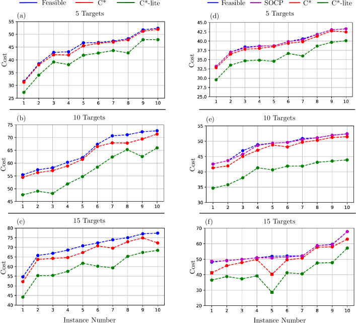
Figure 5: Lower-bound costs of C^∗ and C^∗-lite as compared to the feasible costs for instances from the first set (left) and the second set (right). The SOCP costs are also included for instances from the second set. In (f), square markers indicates the unsuccessful cases. Note how C^∗ gives tight lower-bounds to the feasible costs, and how the bounds from C^∗-lite although weaker, is not too far off.

V-D Varying the Number of Targets

In this section, we will see how changing the number of targets affects the tightness of bounds as well as the run-times for C^∗ and C^∗-lite on average. Once again, we also consider the SOCP formulation when looking at instances within the second set.

The closeness of the costs from the SOCP as well as both the bounds, from the feasible costs can be quantified by finding their $\%$ deviation from the feasible costs. The run-time of C^∗ and C^∗-lite can be separated into two parts. The first part is the time to relax the MT-TSP and generate the underlying graph for the relaxed problem. This run-time will be referred to as graph generation R.T.. The second part is the time to solve the GTSP to optimality on the generated graph. This run-time, when added to the graph generation R.T., gives the total run-time which will be referred to as total R.T.. For the SOCP formulation, the run-time is the time taken to find the optimal solution to the MT-TSP. This run-time will also be referred to as total R.T..

In Fig. 6 (a), we consider all the instances from the first set. The average $\%$ deviation for instances with 5 targets, 10 targets, and 15 targets are considered for C^∗ and C^∗-lite. In (b), we consider all the instances from the second set except for the outliers (instance-1 and instance-5 from the 15 target instances where at least one of the three approaches terminated due to memory constraints). Like (a), we consider the average $\%$ deviation for instances with 5 targets, 10 targets, and 15 targets for C^∗, C^∗-lite, and SOCP.

From both Fig. 6 (a) and (b), we see that the $\%$ deviation for C^∗ and C^∗-lite increases as the number of targets are increased. This is to be expected since the the discontinuities at the time intervals where each target is visited in the optimal solution to the relaxed MT-TSP, adds up with every additional target. However, the $\%$ deviation for C^∗ is small and only increases slightly when the number of targets are increased as compared to C^∗-lite, where both the $\%$ deviation and its increase is significantly higher. One can easily see that this happens as a result of using lower-bounds to the SFT during graph generation. Note how even for 15 targets, the $\%$ deviation is on average $\approx$4$\%$ for C^∗, in both (a) and (b). Finally, the $\%$ deviation for SOCP is very small indicating that the feasible costs obtained were on average, very close to the optimal cost. Note that the SOCP cost does not depend on the number of targets as it aims to find the optimum.

In Fig. 7 (a) and (b), we consider the same instances as Fig. 6 (a) and (b), respectively. For both (a) and (b), we consider the average graph generation R.T. and total R.T. for instances with 5 targets, 10 targets, and 15 targets for C^∗ and C^∗-lite. Additionally, we consider the average total R.T. for SOCP in (b).

From Fig. 7 (a) and (b), we see how the graph generation R.T. for C^∗-lite is significantly smaller than it is for C^∗ as one would expect. As the number of targets are increased, notice how the difference in this run-time between C^∗ and C^∗-lite grows. However, it must be noted that the graph generation R.T. is small relative to the total R.T. for both C^∗ and C^∗-lite. Also, note that the total R.T. is mostly similar for C^∗-lite and C^∗, with it being lower for C^∗-lite for lower number of targets, and it being lower for C^∗ when the number of targets get larger. Although the total R.T. for both C^∗ and C^∗-lite clearly increases with more targets, the runtime to solve the underlying GTSP is much more affected by the increase in targets than the graph generation R.T. since GTSP is NP-hard. Finally, observe how the total R.T. for SOCP is significantly smaller than it is for both C^∗ and C^∗-lite for instances with 5 targets and 10 targets, but then becomes an order of magnitude larger as the number of targets are increased to 15.

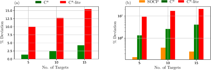
Figure 6: Plots showing how for C^∗ and C^∗-lite, the lower-bounding costs on average, deviates from the feasible costs as the number of targets are varied. Instances from the first and second set were considered for (a) and (b), respectively. Note how the $\%$ deviation for C^∗ is $\approx$4$\%$ for 15 targets, in both the plots. The $\%$ deviation of the SOCP costs in (b) indicates how the optimal costs on average, deviates from the feasible costs by less than 1$\%$.

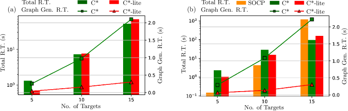
Figure 7: Plots comparing the average run-times of C^∗ and C^∗-lite as the number of targets varies, for instances from the first and second set, as shown in (a) and (b), respectively. The run-times of SOCP in (b) shows how it is on average, almost an order of magnitude faster than C^∗ and C^∗-lite for up to 10 targets, but an order of magnitude slower for 15 targets.

V-E Varying the Discretization

In this section, we will show how the bound tightness as well as the run-times for C^∗ and C^∗-lite on average, gets affected when varying the number of intervals that discretizes $T$. We will also show that in cases where C^∗ or C^∗-lite is unsuccessful, tight bounds can still be obtained by reducing the number of discrete intervals.

We vary the discretization as follows. We start off at lvl-1 where $T$ is discretized into 20 uniform intervals of duration 5. Then for lvl-2, we double the number of intervals so that each interval in lvl-1 contains two intervals in lvl-2. We repeat the process of doubling the intervals until we reach lvl-4. Note that since the duration from all the time-windows adds up to $T/5$ for each target for all our instances, only a fifth of number of intervals are used when generating the graph. All of this is illustrated in Table. I.

Discretization Level	lvl-1	lvl-2	lvl-3	lvl-4
Intervals in Time-Horizon	20	40	80	160
Intervals from Time-Windows	4	8	16	32
Interval Duration	5	2.5	1.25	0.625

TABLE I: Information about the discretization levels.

In Fig. 8 (a) and (b), we consider all the 60 instances except for the two instances we disregarded in the last section. From (a), we see how higher discretizations produces tighter bounds for both C^∗ and C^∗-lite as one would expect. Note that the average $\%$ deviation is significantly more affected for C^∗-lite as compared to C^∗ here. Also, note that the average $\%$ deviation for C^∗-lite at lvl-4 is still higher than it is for C^∗ at lvl-1. Finally, note that the rate at which both the bounds improve, decreases at higher discretizations. From (b), we see how both the run-times increases with higher discretization. The increase in graph generation R.T. is more significant for C^∗ as compared to C^∗-lite. Also, it is very close for C^∗ at lvl-1 and C^∗-lite at lvl-4. However, note that the run-time to solve GTSP on the generated graph, and its increase with higher discretizations, is significantly higher than they are for graph generation R.T. for both bounds. The total R.T. is similar for both C^∗ and C^∗-lite with it being higher for C^∗ at lvl-1 and lvl-2, but then it becoming higher for C^∗-lite at lvl-3 and lvl-4.

Now, we will discuss how reducing the discretization level can give tight lower-bounds whenever C^∗ or C^∗-lite is unsuccessful. In Fig. 9, we consider the 10 instances for 15 targets, within the second set. In (a) and (b), we plot the cost from C^∗ and C^∗-lite respectively, for the four levels of discretization, for each instance. Previously, we saw how at lvl-4, C^∗ was unsuccessful for instance-1 and instance-5, and how C^∗-lite was unsuccessful for instance-5. However, now we can see how for both C^∗ and C^∗-lite, lvl-3 and below is successful for all instances and how lvl-3 provides a tighter lower-bound in all the cases where lvl-4 was unsuccessful. In (a), note how even lvl-2 gives very close, or even better bounds than lvl-4 for instances, 1 and 5.

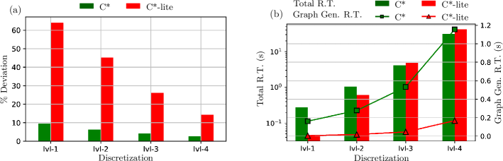
Figure 8: (a) The average $\%$ deviation of the lower-bound costs of C^∗ and C^∗-lite from the feasible costs as the discretization level is varied. (b) The average run-times of C^∗ and C^∗-lite as the discretization level is varied. Note how in (a), C^∗ at lvl-1 has lower $\%$ deviation than C^∗-lite at lvl-4. Also note how in (b), the graph generation R.T. is very close for C^∗ at lvl-1 and C^∗-lite at lvl-4.

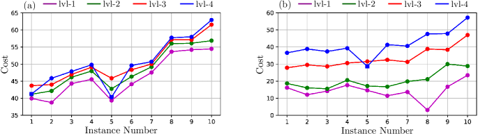
Figure 9: Lower-bound costs of C^∗ (a) and C^∗-lite (b) for all discretization levels, for each 15 targets instance in the second set. Square markers indicates the unsuccessful cases. In (a), lvl-4 is unsuccessful for instance-1 and instance-5. In (b), lvl-4 is unsuccessful for instance-5. Note how for all the instances where lvl-4 is unsuccessful in (a) and (b), lvl-3 is successful and give tighter bounds. Also observe how in (a), even lvl-2 gives similar or tighter bounds for instances where lvl-4 is unsuccessful.

V-F Obtaining Feasible Solutions from C^∗ and C^∗-lite

In this section, we attempt to construct feasible solutions to the MT-TSP from the lower-bounds obtained from C^∗ and C^∗-lite. We also evaluate how good the costs are for these solutions. Clearly, if the number of intervals that discretizes $T$ goes to infinity, the lower-bounds converge to the optimum. However, this is impossible to implement, and is computationally infeasible. Hence, we will fix the discretization at lvl-4.

To construct feasible solutions from lower-bounds, we simply take the order in which the targets were visited in the lower-bounding solution, and construct the minimum cost tour for the agent for the same order, without violating the time-window constraints, or the maximum agent speed constraint. In the cases where such a tour cannot be constructed, we say a feasible solution cannot be constructed from the lower-bound from C^∗ or C^∗-lite.

In Table. II, we consider all the 60 instances except for the 2 instances where at least one of C^∗ and C^∗-lite was unsuccessful (same instances as in Fig. 8). Here, the Success Rate illustrates the percentage of instances for which we were able to construct a feasible solution from the lower-bound. From these instances, we compare the new feasible solutions against the original ones to see the percentage of instances for which they match. This is given by $\%$ Match in the table. Finally, from all the instances where the solutions did not match, we average the costs of both the feasible solutions originally obtained, as well as the ones that were newly constructed, and find the $\%$ deviation of the new average cost from the original average cost. This is given by $\%$ Dev-Mismatch.

We see how the success rate is close to a 100$\%$ for both C^∗ and C^∗-lite. If we cannot construct a feasible solution using the lower-bound from C^∗, then we might be able to, using the one from C^∗-lite, or vice versa. Hence, for at least 98$\%$ of the instances, we were able to construct feasible solutions using lower-bounds from the C^∗ variants. Also, note how the $\%$ match is significantly higher for C^∗. This is to expected since we find the optimal solution to the SFT when using C^∗. Finally, we can see how the $\%$ dev-mismatch is very close to 0$\%$ for both C^∗ and C^∗-lite, with the new costs being slightly larger than the original ones on average for both bounds.

	Success Rate ($\%$)	$\%$ Match	$\%$ Dev-Mismatch
C*	96.55	64.29	0.21
C*-lite	98.28	47.37	0.27

TABLE II: Table illustrating the success rate of constructing feasible solutions from lower-bounds obtained from C^∗ and C^∗-lite, and how these feasible solutions compare with the originally found feasible solutions.

VI Conclusion and Future Work

We presented C^∗, an approach that finds lower-bounds to the MT-TSP. To use C^∗, we solved a new problem called the Shortest Feasible Travel (SFT). We also introduced C^∗-lite, where C^∗ is modified such that the solutions to the SFT are replaced with simple and easy to compute lower-bounds. We proved that our approaches provide lower-bounds to the MT-TSP, and presented extensive numerical results to corroborate the performance of both C^∗ and C^∗-lite. Finally, we showed how feasible solutions can be constructed most of the time from the lower-bounds obtained from C^∗ and C^∗-lite.

One of the challenges in this paper was the computational burden that comes with increasing the number of targets. This arises from solving the GTSP, where computational complexity heavily depends on the number of nodes in the generated graph. Finding a way to circumvent this will allow us to successfully find tight bounds for larger number of targets. C^∗ can be generalized in several ways. A natural extension would be to account for multiple agents with different depot locations. This can be further generalized by adding stationary or moving obstacles.

VII Appendix

VII-A Finding Earliest Feasible Arrival Time

Figure 10: Example 1

Let $s_{1}$ and $s_{2}$ be two targets moving along trajectories $\pi_{s_{1}}$ and $\pi_{s_{2}}$. Let the trajectory-point $\pi_{s}(t)$ for some target $s$ at time $t$ be denoted by the tuple $(x,y)$, where $x$ and $y$ are the coordinates of the position occupied by $s$ at time $t$, with respect to a fixed standard basis. Also, let $\dot{x}$ and $\dot{y}$ denote the time derivative of $x$ and $y$ respectively. We then consider the following cases.

VII-A1 $\pi_{s_{1}}$ and $\pi_{s_{2}}$ are linear trajectories

Given $\pi_{s_{1}}$ and $\pi_{s_{2}}$, we aim to find $e(t_{i})$ for some time $t_{i}$. Let $t_{i}\geq t_{1}$ and $t\geq t_{2}$ where $t_{2}$ is chosen such that $e(t_{i})\geq t_{2}$. Without loss of generality, consider example 1 illustrated in Fig 10, showing the part of $\pi_{s_{1}}$ from time $t_{1}$ onward and the part of $\pi_{s_{2}}$ from time $t_{2}$ onward. Note that $\pi_{s_{1}}(t_{i})\equiv(a_{x},a_{y})$ and $\pi_{s_{2}}(t)\equiv(x,y)$. Let $\pi_{s_{1}}(t_{1})\equiv(a_{x_{1}},a_{y_{1}})$ and $\pi_{s_{2}}(t_{2})\equiv(x_{2},y_{2})$. The following equations then describes the motion of $s_{1}$ and $s_{2}$ from times $t_{1}$ and $t_{2}$ onward, respectively.

$$a_{x}=a_{x_{1}}+\dot{a_{x}}(t_{i}-t_{1})$$ (1)

$$a_{y}=a_{y_{1}}+\dot{a_{y}}(t_{i}-t_{1})$$ (2)

$$x=x_{2}+\dot{x}(t-t_{2})$$ (3)

$$y=y_{2}+\dot{y}(t-t_{2})$$ (4)

The distance between $(a_{x},a_{y})$ and $(x,y)$ is then given by $\sqrt{(x-a_{x})^{2}+(y-a_{y})^{2}}$. Also, using lemma 2 we want the agent to travel at speed $v_{max}$ to obtain $e(t_{i})$. Hence, we want $t$ that satisfies

$$\sqrt{(x-a_{x})^{2}+(y-a_{y})^{2}}=v_{max}(t-t_{i})$$ (5)

Squaring both sides, we obtain

$$(x-a_{x})^{2}+(y-a_{y})^{2}=v_{max}^{2}(t-t_{i})^{2}$$ (6)

Substituting (1), (2), (3), (4) into (6), and rearranging the terms, we get

$$(\dot{x}t+C_{1})^{2}+(\dot{y}t+C_{2})^{2}=v_{max}^{2}(t-t_{i})^{2}$$ (7)

where

$$C_{1}=-\dot{a_{x}}t_{i}+C_{1}^{\prime}$$

$$C_{2}=-\dot{a_{y}}t_{i}+C_{2}^{\prime}$$

$$C_{1}^{\prime}=x_{2}-\dot{x}t_{2}-a_{x_{1}}+\dot{a_{x}}t_{1}$$

$$C_{2}^{\prime}=y_{2}-\dot{y}t_{2}-a_{y_{1}}+\dot{a_{y}}t_{1}$$

After extensive algebra, we finally get the following.

$$At^{2}+B(t_{i})t+C(t_{i})=0$$ (8)

where

$$A=\dot{x}^{2}+\dot{y}^{2}-v_{max}^{2}$$

$$B(t_{i})=2B^{\prime}t_{i}+2C^{\prime}$$

$$C(t_{i})=A^{\prime}t_{i}^{2}-D^{\prime}t_{i}+E^{\prime}$$

$$B^{\prime}=-\dot{a_{x}}\dot{x}-\dot{a_{y}}\dot{y}+v_{max}^{2}$$

$$C^{\prime}=C_{1}^{\prime}\dot{x}+C_{2}^{\prime}\dot{y}$$

$$A^{\prime}=\dot{a_{x}}^{2}+\dot{a_{y}}^{2}-v_{max}^{2}$$

$$D^{\prime}=2\dot{a_{x}}C_{1}^{\prime}+2\dot{a_{y}}C_{2}^{\prime}$$

$$E^{\prime}=C_{1}^{\prime 2}+C_{2}^{\prime 2}$$

One of the two roots that satisfies (8) is then the EFAT $e(t_{i})$. These roots can be obtained using the quadratic formula as shown below.

$$t=\frac{-B(t_{i})\pm\sqrt{B(t_{i})^{2}-4AC(t_{i})}}{2A}$$ (9)

VII-A2 $\pi_{s_{1}}$ and $\pi_{s_{2}}$ are piecewise-linear trajectories

Without loss of generality, we will use example 2 illustrated in Fig. 11 to explain the algorithm to find $e(t_{i})$.

First, break $[t_{d},t_{g}]$ into the sub-intervals $[t_{d},t_{e}]$, $[t_{e},t_{f}]$, and $[t_{f},t_{g}]$. Find $\min_{t\geq t_{i}}\{t_{e},t_{f},t_{g}\}$. Suppose $t=t_{f}$. Then clearly, the agent cannot arrive at $s_{2}$ during any time $t\leq t_{e}$ by departing from $s_{1}$ at time $t_{i}$. Now, check if the agent can travel feasibly from $\pi_{s_{1}}(t_{i})$ to $\pi_{s_{2}}(t_{f})$. Suppose this is true. Then $e(t_{i})$ must lie within $(t_{e},t_{f}]$. By considering the linear trajectory-intervals $\pi_{s_{1}}[t_{b},t_{c}]$ and $\pi_{s_{2}}[t_{e},t_{f}]$ as the input, we can find $e(t_{i})$ using the approach derived in VII-A1. If not true, then using lemma 1, the agent cannot arrive at $s_{2}$ during any time $t\leq t_{f}$ by departing from $s_{1}$ at time $t_{i}$. Hence, repeat the process again by checking if the agent can travel feasibly from $\pi_{s_{1}}(t_{i})$ to $\pi_{s_{2}}(t_{g})$ and following the remaining steps.

Figure 11: Example 2

VII-B Finding Latest Feasible Departure Time

Once again, we consider the following cases.

VII-B1 $\pi_{s_{1}}$ and $\pi_{s_{2}}$ are linear trajectories

In VII-A1, we saw that given $t_{i}$, one of the roots that satisfies (8) is the EFAT $e(t_{i})$. Also, from lemma 5, we saw that $t=e(t_{i})\iff l(t)=t_{i}$. Hence, given a value of $t$, we seek to find $t_{i}$ such that $t$ satisfies (8). To solve this, note that (8) can be expanded as follows.

$$At^{2}+(2B^{\prime}t_{i}+2C^{\prime})t+(A^{\prime}t_{i}^{2}-D^{\prime}t_{i}+E^{\prime})=0$$ (10)

By rearranging the terms in (10) we get the below equation.

$$A^{\prime}t_{i}^{2}+(2B^{\prime}t-D^{\prime})t_{i}+(At^{2}+2C^{\prime}t+E^{\prime})=0$$ (11)

(11) can then be represented simply as

$$A^{\prime}t_{i}^{2}+H(t)t_{i}+I(t)=0$$ (12)

Hence, one of the two roots that satisfies 12 is the LFDT $l(t)$. Like previously shown, these roots can be obtained using the quadratic formula below.

$$t_{i}=\frac{-H(t)\pm\sqrt{H(t)^{2}-4A^{\prime}I(t)}}{2A^{\prime}}$$ (13)

VII-B2 $\pi_{s_{1}}$ and $\pi_{s_{2}}$ are piecewise-linear trajectories

Without loss of generality, we will use example 3 illustrated in Fig. 12, similar to example 2, to explain the algorithm to find $l(t)$.

First, break $[t_{a},t_{d}]$ into the sub-intervals $[t_{a},t_{b}]$, $[t_{b},t_{c}]$, and $[t_{c},t_{d}]$. Find $\max_{t_{i}\leq t}\{t_{a},t_{b},t_{c}\}$. Suppose $t_{i}=t_{b}$. Then clearly, the agent cannot arrive at $s_{2}$ at time $t$ by departing from $s_{1}$ during any time $t_{i}\geq t_{c}$. Now, check if the agent can travel feasibly from $\pi_{s_{1}}(t_{b})$ to $\pi_{s_{2}}(t)$. Suppose this is true. Then $l(t)$ must lie within $[t_{b},t_{c})$. By considering the linear trajectory-intervals $\pi_{s_{1}}[t_{b},t_{c}]$ and $\pi_{s_{2}}[t_{f},t_{g}]$ as the input, we can find $l(t)$ using the approach derived in VII-B1. If not true, then using lemma 3, the agent cannot arrive at $s_{2}$ at time $t$ by departing from $s_{1}$ during any time $t_{i}\geq t_{b}$. Hence, repeat the process again by checking if the agent can travel feasibly from $\pi_{s_{1}}(t_{a})$ to $\pi_{s_{2}}(t)$ and following the remaining steps.

Figure 12: Example 3

VII-C Finding Stationary Points of $e(t_{i})-t_{i}$

Consider the same case as in VII-A1 where $\pi_{s_{1}}$ and $\pi_{s_{2}}$ are linear trajectories. From here onward, we use $t$ to represent the functions of $t_{i}$ defined in (9) as opposed to a free variable. By differentiating (9) with respect to $t_{i}$, we can find an expression for $\frac{dt}{dt_{i}}$ as follows.

$$\frac{dt}{dt_{i}}=\frac{1}{2A}\left[-\frac{d}{dt_{i}}B(t_{i})\pm\frac{2B(t_{i})\frac{d}{dt_{i}}B(t_{i})-4A\frac{d}{dt_{i}}C(t_{i})}{2\sqrt{B(t_{i})^{2}-4AC(t_{i})}}\right]=$$

$$\frac{1}{2A}\left[-2B^{\prime}\pm\frac{2(2B^{\prime}t_{i}+2C^{\prime})(2B^{\prime})-4A(2A^{\prime}t_{i}-D^{\prime})}{2\sqrt{(2B^{\prime}t_{i}+2C^{\prime})^{2}-4A(A^{\prime}t_{i}^{2}-D^{\prime}t_{i}+E^{\prime})}}\right]$$

After further simplification, we get

$$\frac{dt}{dt_{i}}=\frac{1}{A}\left[-B^{\prime}\pm\frac{2B^{\prime}(B^{\prime}t_{i}+C^{\prime})-A(2A^{\prime}t_{i}-D^{\prime})}{2\sqrt{(B^{\prime}t_{i}+C^{\prime})^{2}-A(A^{\prime}t_{i}^{2}-D^{\prime}t_{i}+E^{\prime})}}\right]$$ (14)

To find the stationary points of $t-t_{i}$, we set $\frac{d}{dt_{i}}(t-t_{i})=0$ which then gives us

$$\frac{dt}{dt_{i}}-1=0\implies\frac{dt}{dt_{i}}=1$$ (15)

Substituting (14) into (15), we get the following.

$$\frac{1}{A}\left[-B^{\prime}\pm\frac{2B^{\prime}(B^{\prime}t_{i}+C^{\prime})-A(2A^{\prime}t_{i}-D^{\prime})}{2\sqrt{(B^{\prime}t_{i}+C^{\prime})^{2}-A(A^{\prime}t_{i}^{2}-D^{\prime}t_{i}+E^{\prime})}}\right]=1$$

which can be rearranged as

$$(A+B^{\prime})=\pm\frac{2B^{\prime}(B^{\prime}t_{i}+C^{\prime})-A(2A^{\prime}t_{i}-D^{\prime})}{2\sqrt{(B^{\prime}t_{i}+C^{\prime})^{2}-A(A^{\prime}t_{i}^{2}-D^{\prime}t_{i}+E^{\prime})}}$$ (16)

Note that $(B^{\prime}t_{i}+C^{\prime})^{2}-A(A^{\prime}t_{i}^{2}-D^{\prime}t_{i}+E^{\prime})\geq 0$ for all $t_{i}$. If $(B^{\prime}t_{i}+C^{\prime})^{2}-A(A^{\prime}t_{i}^{2}-D^{\prime}t_{i}+E^{\prime})=0$ for some $t_{i}$, then it means both $s_{1}$ and $s_{2}$ occupies the same position at time $t_{i}$. In this case, the function $t-t_{i}$ becomes $0$ and takes a sharp turn ($\frac{d}{dt_{i}}(t-t_{i})$ becomes undefined) at $t_{i}$. However, if $(B^{\prime}t_{i}+C^{\prime})^{2}-A(A^{\prime}t_{i}^{2}-D^{\prime}t_{i}+E^{\prime})>0$, we get the following by squaring both sides of (16) and multiplying the denominator on both sides.

$$4(A+B^{\prime})^{2}((B^{\prime}t_{i}+C^{\prime})^{2}-A(A^{\prime}t_{i}^{2}-D^{\prime}t_{i}+E^{\prime}))$$

$$= (2B^{\prime}(B^{\prime}t_{i}+C^{\prime})-A(2A^{\prime}t_{i}-D^{\prime}))^{2}$$

After extensive algebra, we finally get the following.

$$Pt_{i}^{2}+Qt_{i}+R=0$$ (17)

where

$$\begin{split}P&=4(A+B^{\prime})^{2}(B^{\prime 2}-AA^{\prime})-4B^{\prime 4}\\ &-(4A^{2}A^{\prime 2}-8AA^{\prime}B^{\prime 2})\end{split}$$

$$\begin{split}Q&=4(A+B^{\prime})^{2}(2B^{\prime}C^{\prime}+AD^{\prime})-8B^{\prime 3}C^{\prime}\\ &-(4AB^{\prime 2}D^{\prime}-8AA^{\prime}B^{\prime}C^{\prime}-4A^{2}A^{\prime}D^{\prime})\end{split}$$

$$R =4(A+B^{\prime})^{2}(C^{\prime 2}-AE^{\prime})-4B^{\prime 2}C^{\prime 2}$$

$$-(4AB^{\prime}C^{\prime}D^{\prime}+A^{2}D^{\prime 2})$$

The values of $t_{i}$ that satisfies the two equations in (16) can be obtained by solving for the two roots that satisfies (17). These roots can once again, be obtained using the quadratic formula given below.

$$t_{i}=\frac{-Q\pm\sqrt{Q^{2}-4PR}}{2P}$$ (18)

VII-D Second Order Cone Program (SOCP) Formulation

In this section, we explain the SOCP formulation for the special case of the MT-TSP where targets follow linear trajectories. Our formulation is very similar to the one presented in [24], with a few changes made to accommodate the new objective which is to minimize the time taken by the agent to complete the tour, as opposed to minimizing the length of the path traversed by the agent.

To ensure that the trajectory of the agent starts and ends at the depot, we do the following: Given the depot $d$ and a set of $n-1$ targets $\{1,\cdots,n-1\}$, we define a new stationary target $n$ which acts as a copy of $d$. This is achieved by fixing $n$ at the same position as $d$. We then define constraints so that the agent’s trajectory starts from $d$ and ends at $n$. To find the optimal solution to the MT-TSP, we then seek to minimize the time at which $n$ is visited by the agent.

Let $S\equiv\{1,\cdots,n\}$ and $S_{d}\equiv\{d\}\cup S$. We use the same family of decision variables as in [24] where $x_{i,j}\in\{0,1\}$ indicates the decision of sending the agent from target $i$ to target $j$ ($x_{i,j}=1$ if yes. No otherwise), and $t_{i}\in\mathbb{R}$ describes the arrival time of the agent at target $i$ (or depot).

Our objective is to minimize the time at which the agent arrives at target $n$ as shown below.

$$\min t_{n}$$ (19)

Each target $j$ must be visited once by the agent:

$$\sum_{i\in S_{d}:i\neq j}x_{i,j}=1,\;\forall\>j\in S$$ (20)

The agent can start only once from the depot:

$$\sum_{j\in S}x_{d,j}\leq 1$$ (21)

Flow conservation is ensured by:

$$\sum_{i\in S_{d}:i\neq j}x_{i,j}\geq\sum_{i\in S:i\neq j}x_{j,i},\;\forall\>j\in S$$ (22)

The agent must visit each target within its assigned time-window. Note that, for the depot $d$ and the target $n$, we assign the time-window to be the entire time-horizon $T$:

$$t_{l}^{j}\leq t_{j}\leq t_{u}^{j},\;\forall\>j\in S_{d}$$ (23)

As shown in [24], real auxiliary variables $c_{i,j}^{x}$ and $c_{i,j}^{y}$ for the $x-$ and $y-$ components of the Euclidean distance are introduced as follows:

$$\begin{split}&c_{d,j}^{x}-\left(\left(x_{l}^{j}+t_{j}\frac{\Delta{x_{j}}}{\Delta{t_{j}}}-t_{l}^{j}\frac{\Delta{x_{j}}}{\Delta{t_{j}}}\right)-d_{x}\right)=0,\\ &\forall\>j\in S\end{split}$$ (24)

$$\begin{split}&c_{d,j}^{y}-\left(\left(y_{l}^{j}+t_{j}\frac{\Delta{y_{j}}}{\Delta{t_{j}}}-t_{l}^{j}\frac{\Delta{y_{j}}}{\Delta{t_{j}}}\right)-d_{y}\right)=0,\\ &\forall\>j\in S\end{split}$$ (25)

$$\begin{split}c_{i,j}^{x}&-\left(\left(x_{l}^{j}+t_{j}\frac{\Delta{x_{j}}}{\Delta{t_{j}}}-t_{l}^{j}\frac{\Delta{x_{j}}}{\Delta{t_{j}}}\right)-\left(x_{l}^{i}+t_{i}\frac{\Delta{x_{i}}}{\Delta{t_{i}}}-t_{l}^{i}\frac{\Delta{x_{i}}}{\Delta{t_{i}}}\right)\right)\\ &=0,\;\forall\>i\in S,j\in S:i\neq j\end{split}$$ (26)

$$\begin{split}c_{i,j}^{y}&-\left(\left(y_{l}^{j}+t_{j}\frac{\Delta{y_{j}}}{\Delta{t_{j}}}-t_{l}^{j}\frac{\Delta{y_{j}}}{\Delta{t_{j}}}\right)-\left(y_{l}^{i}+t_{i}\frac{\Delta{y_{i}}}{\Delta{t_{i}}}-t_{l}^{i}\frac{\Delta{y_{i}}}{\Delta{t_{i}}}\right)\right)\\ &=0,\;\forall\>i\in S,j\in S:i\neq j\end{split}$$ (27)

Here, for some target $i$, $(x_{l}^{i},y_{l}^{i})$ represents the coordinates of $i$ at time $t_{l}^{i}$ and $(x_{u}^{i},y_{u}^{i})$ represents the coordinates of $i$ at time $t_{u}^{i}$. Also, $\Delta{x_{i}}=x_{u}^{i}-x_{l}^{i}$, $\Delta{y_{i}}=y_{u}^{i}-y_{l}^{i}$, and $\Delta{t_{i}}=t_{u}^{i}-t_{l}^{i}$. Finally, $(d_{x},d_{y})$ denotes the coordinates of the depot $d$.

The following conditions requires that if the agent travels between any two targets or the depot and a target, this travel must be feasible:

$$\begin{split}&a_{i,j}\leq v_{max}(t_{j}-t_{i}+T(1-x_{i,j})),\\ &\forall\>i\in S_{d},j\in S:i\neq j\end{split}$$ (28)

$$a_{i,j}\geq 0,\;\forall\>i\in S_{d},j\in S:i\neq j$$ (29)

The below conditions are needed to formulate the cone constraints:

$$\begin{split}&\overline{a}_{i,j}=a_{i,j}+R(1-x_{i,j}),\;\forall\>i\in S_{d},j\in S:i\neq j\end{split}$$ (30)

Where given the square area with fixed side length $L$ that contains all the moving targets and the depot, $R=\sqrt{2}L$ is the length of the square’s diagonal.

Finally, the cone constraints are given as:

$$(c_{i,j}^{x})^{2}+(c_{i,j}^{y})^{2}\leq(\overline{a}_{i,j})^{2},\;\forall\>i\in S_{d},j\in S:i\neq j$$ (31)

The agent must visit $n$ only after visiting all the other targets:

$$t_{n}\geq t_{j},\;\forall\>j\in S_{d}$$ (32)

Remark 5.

Although (28) prevents subtours in most cases, they can still arise very rarely when two or more target trajectories intersect at a time common to their time-windows. The constraints defined by (33) prevents subtours for the two target case. However for more than two targets, we will need additional subtour elimination constraints:

$$x_{i,j}+x_{j,i}\leq 1,\;\forall\>i\in S,j\in S:i\neq j$$ (33)

References

- [1] Jean-Marie Bourjolly, Ozgur Gurtuna, and Aleksander Lyngvi. On-orbit servicing: a time-dependent, moving-target traveling salesman problem. International Transactions in Operational Research, 13(5):461–481, 2006.
- [2] Barry L Brumitt and Anthony Stentz. Dynamic mission planning for multiple mobile robots. In Proceedings of IEEE International Conference on Robotics and Automation, volume 3, pages 2396–2401. IEEE, 1996.
- [3] Prasad Chalasani and Rajeev Motwani. Approximating capacitated routing and delivery problems. SIAM Journal on Computing, 28(6):2133–2149, 1999.
- [4] Omar Cheikhrouhou, Anis Koubâa, and Anis Zarrad. A cloud based disaster management system. Journal of Sensor and Actuator Networks, 9(1):6, 2020.
- [5] Nitin S Choubey. Moving target travelling salesman problem using genetic algorithm. International Journal of Computer Applications, 70(2), 2013.
- [6] Jesus Conesa-Muñoz, Gonzalo Pajares, and Angela Ribeiro. Mix-opt: A new route operator for optimal coverage path planning for a fleet in an agricultural environment. Expert Systems with Applications, 54:364–378, 2016.
- [7] Rodrigo S de Moraes and Edison P de Freitas. Experimental analysis of heuristic solutions for the moving target traveling salesman problem applied to a moving targets monitoring system. Expert Systems with Applications, 136:392–409, 2019.
- [8] Brendan Englot, Tuhin Sahai, and Isaac Cohen. Efficient tracking and pursuit of moving targets by heuristic solution of the traveling salesman problem. In 52nd ieee conference on decision and control, pages 3433–3438. IEEE, 2013.
- [9] Carlos Groba, Antonio Sartal, and Xosé H Vázquez. Solving the dynamic traveling salesman problem using a genetic algorithm with trajectory prediction: An application to fish aggregating devices. Computers & Operations Research, 56:22–32, 2015.
- [10] Andy M Ham. Integrated scheduling of m-truck, m-drone, and m-depot constrained by time-window, drop-pickup, and m-visit using constraint programming. Transportation Research Part C: Emerging Technologies, 91:1–14, 2018.
- [11] Mikael Hammar and Bengt J Nilsson. Approximation results for kinetic variants of tsp. In Automata, Languages and Programming: 26th International Colloquium, ICALP’99 Prague, Czech Republic, July 11–15, 1999 Proceedings 26, pages 392–401. Springer, 1999.
- [12] Michael Hassoun, Shraga Shoval, Eran Simchon, and Liron Yedidsion. The single line moving target traveling salesman problem with release times. Annals of Operations Research, 289:449–458, 2020.
- [13] Keld Helsgaun. An effective implementation of the lin–kernighan traveling salesman heuristic. European journal of operational research, 126(1):106–130, 2000.
- [14] Christopher S Helvig, Gabriel Robins, and Alex Zelikovsky. The moving-target traveling salesman problem. Journal of Algorithms, 49(1):153–174, 2003.
- [15] Q Jiang, R Sarker, and H Abbass. Tracking moving targets and the non-stationary traveling salesman problem. Complexity International, 11(2005):171–179, 2005.
- [16] Gilbert Laporte, Hélène Mercure, and Yves Nobert. Generalized travelling salesman problem through n sets of nodes: the asymmetrical case. Discrete Applied Mathematics, 18(2):185–197, 1987.
- [17] Yuanchang Liu and Richard Bucknall. Efficient multi-task allocation and path planning for unmanned surface vehicle in support of ocean operations. Neurocomputing, 275:1550–1566, 2018.
- [18] DO Marlow, P Kilby, and GN Mercer. The travelling salesman problem in maritime surveillance–techniques, algorithms and analysis. In Proceedings of the international congress on modelling and simulation, pages 684–690, 2007.
- [19] Alaleh Maskooki and Markku Kallio. A bi-criteria moving-target travelling salesman problem under uncertainty. European Journal of Operational Research, 2023.
- [20] Charles E Noon and James C Bean. An efficient transformation of the generalized traveling salesman problem. INFOR: Information Systems and Operational Research, 31(1):39–44, 1993.
- [21] Paul Oberlin, Sivakumar Rathinam, and Swaroop Darbha. Today’s traveling salesman problem. IEEE robotics & automation magazine, 17(4):70–77, 2010.
- [22] Joel L Ryan, T Glenn Bailey, James T Moore, and William B Carlton. Reactive tabu search in unmanned aerial reconnaissance simulations. In 1998 Winter Simulation Conference. Proceedings (Cat. No. 98CH36274), volume 1, pages 873–879. IEEE, 1998.
- [23] Hussain Aziz Saleh and Rachid Chelouah. The design of the global navigation satellite system surveying networks using genetic algorithms. Engineering Applications of Artificial Intelligence, 17(1):111–122, 2004.
- [24] Anke Stieber and Armin Fügenschuh. Dealing with time in the multiple traveling salespersons problem with moving targets. Central European Journal of Operations Research, 30(3):991–1017, 2022.
- [25] Ukbe Ucar and Selçuk Kürşat Işleyen. A meta-heuristic solution approach for the destruction of moving targets through air operations. International Journal of Industrial Engineering, 26(6), 2019.
- [26] Saravanan Venkatachalam, Kaarthik Sundar, and Sivakumar Rathinam. A two-stage approach for routing multiple unmanned aerial vehicles with stochastic fuel consumption. Sensors, 18(11):3756, 2018.
- [27] Yixuan Wang and Nuo Wang. Moving-target travelling salesman problem for a helicopter patrolling suspicious boats in antipiracy escort operations. Expert Systems with Applications, 213:118986, 2023.
- [28] Zhong Yu, Liang Jinhai, Gu Guochang, Zhang Rubo, and Yang Haiyan. An implementation of evolutionary computation for path planning of cooperative mobile robots. In Proceedings of the 4th World Congress on Intelligent Control and Automation (Cat. No. 02EX527), volume 3, pages 1798–1802. IEEE, 2002.
- [29] Wanqing Zhao, Qinggang Meng, and Paul WH Chung. A heuristic distributed task allocation method for multivehicle multitask problems and its application to search and rescue scenario. IEEE transactions on cybernetics, 46(4):902–915, 2015.