Invariants of virtual links and twisted links using affine indices

Abstract.

The affine index polynomial and the $n$-writhe are invariants of virtual knots which are introduced by Kauffman [22] and by Satoh and Taniguchi [25] independently. They are defined by using indices assigned to each classical crossing, which we call affine indices in this paper. We discuss a relationship between the invariants and generalize them to invariants of virtual links. The invariants for virtual links can be also computed by using cut systems. We also introduce invariants of twisted links by using affine indices.

1. Introduction

Virtual links are a generalization of links introduced by Kauffman [20]. They are defined as equivalence classes of link diagrams possibly with virtual crossings, called virtual link diagrams, and they correspond to equivalence classes of Gauss diagrams [20]. They are also in one-to-one correspondence with stable equivalence classes of links in thickened oriented surfaces [3, 17], and with abstract links defined in [17].

The affine index polynomial $P_{K}(t)$ and the $n$-writhe $J_{n}(K)$ $(n\neq 0)$ are invariants of virtual knots which are introduced by Kauffman [22] and by Satoh and Taniguchi [25] independently. They are defined by using indices assigned to each classical crossing, which we call affine indices in this paper. Affine indices are a refinement of indices introduced by Henrich [10] and Im, Lee and Lee [11]. The odd writhe invariant [21], the odd writhe polynomial [4] and the invariants in [10] and [11] are recovered from the affine index polynomial and the $n$-writhe. One of the purposes of this paper is to discuss a relationship between the affine index polynomial and the $n$-writhe (Proposition 5) and generalize them to invariants of virtual links.

For a virtual link diagram $D$, we define the over and under $n$-writhe, $J^{\rm O}_{n}(D)$ and $J^{\rm U}_{n}(D)$, for $n\neq 0$, and over, under and over-under affine index polynomials, $P^{\rm O}_{D}(t)$, $P^{\rm U}_{D}(t)$ and $P^{\rm OU}_{D}(s,t)$. All of these are virtual link invariants (Theorem 7).

Kauffman [23] defined the affine index polynomial $P_{L}(t)$ for a compatible virtual link. For a compatible virtual link, our invariants $P^{\rm O}_{L}(t)$ and $P^{\rm U}_{L}(t)$ are essentially the same with $P_{L}(t)$ (Remark 9).

Another purpose is to give an alternative definition to these invariants, or an alternative method of computing these invariants, using cut systems. A cut system of a virtual link diagram $D$ is a finite set of oriented cut points such that the diagram with the cut points admits an Alexander numbering. Cut systems are used for constructing a checkerboard colorable, a mod-$m$ almost classical or almost classical virtual link diagram from a given virtual link diagram (cf. [14, 15, 16]). Oriented cut points are a generalization of (unoriented) cut points introduced by Dye [6, 7].

Twisted links are also a generalization of links introduced by Bourgoin [1]. They are defined as equivalence classes of link diagrams possibly with virtual crossings and bars, called twisted link diagrams. They are in one-to-one correspondence with stable equivalence classes of links in thickened surfaces, and with abstract links over unoriented surfaces. We introduce invariants of twisted links using affine indices via the double covering method introduced in [18]. In the last section, we introduce another invariant of twisted links using affine indices.

This paper is organized as follows: In Section 2 we recall the notion of virtual knots and links. In Section 3 we recall the $n$-writhe and the affine index polynomial for a virtual knot, and observe a relationship between them. In Section 4 we generalize the invariants to virtual link invariants. In Section 5 we recall the notions of Alexander numberings, oriented cut points and cut systems. Then we discuss an alternative definition of the invariants for virtual knots and links in terms of cut systems. In Section 6 we recall the definition of twisted knots and links, and construct invariants of twisted links via the double covering method. In Section 7 another invariant of twisted links is defined by using the affine indices modulo $2$.

2. Virtual knots and links

A virtual link diagram is a collection of immersed oriented loops in $\mathbb{R}^{2}$ such that the multiple points are transverse double points which are classified into classical crossings and virtual crossings: A classical crossing is a crossing with over/under information as in usual link diagrams, and a virtual crossing is a crossing without over/under information [20]. A virtual crossing is depicted as a crossing encircled with a small circle in oder to distinguish from classical crossings. (Such a circle is not considered as a component of the virtual link diagram.) A classical crossing is also called a positive or negative crossing according to the sign of the crossing as usual in knot theory. A virtual knot diagram is a virtual link diagram with one component.

Generalized Reidemeister moves are local moves depicted in Figure  1: The 3 moves on the top are (classical) Reidemeister moves and the 4 moves on the bottom are so-called virtual Reidemeister moves. Two virtual link diagrams are said to be equivalent if they are related by a finite sequence of generalized Reidemeister moves and isotopies of $\mathbb{R}^{2}$. A virtual link is an equivalence class of virtual link diagrams. A virtual knot is an equivalence class of a virtual knot diagram.

$D$Mk$D^{\prime}$Mk $D$MMM$D^{\prime}$ $D$MMMk$D^{\prime}$ I II III Reidemeister moves

I II III IV Virtual Reidemeister moves

Figure 1. Generalized Reidemeister moves

3. The $n$ writhe and the affine index polynomial of a virtual knot

In this section, we recall two kinds of invariants of virtual knots, the $n$-writhe $J_{n}(K)$ $(n\neq 0)$ due to Satoh and Taniguchi [25] and the affine index polynomial $P_{K}(t)$ due to Kauffman [22]. These two invariants were introduced independently, and it turns out that they are essentially the same invariant.

Let $D$ be a virtual knot diagram and $c$ a classical crossing. The sign of $c$ is denoted by ${\rm sgn}(c)$. Let $D_{c}$ be a virtual link diagram obtained from $D$ by smoothing at $c$.

The left (or right) counting component for $D$ at $c$ means a component of $D_{c}$ which is denoted by $D_{c}^{\rm L}$ (or $D_{c}^{\rm R}$) in Figure 2.

Figure 2. Counting components $D_{c}^{\rm L}$ and $D_{c}^{\rm R}$

The over counting component and the under counting component for $D$ at $c$ mean components of $D_{c}$ which are denoted by $D_{c}^{\rm L}$ and $D_{c}^{\rm R}$ in Figure 3 or 4 according to the sign of $c$. In other words,

$$\begin{array}[]{rrl}D_{c}^{\rm O}=D_{c}^{\rm R},&\quad D_{c}^{\rm U}=D_{c}^{\rm L}&\qquad({\rm sgn}(c)=+1),\\ D_{c}^{\rm O}=D_{c}^{\rm L},&\quad D_{c}^{\rm U}=D_{c}^{\rm R}&\qquad({\rm sgn}(c)=-1).\end{array}$$

Figure 3. Counting components $D_{c}^{\rm O}$ and $D_{c}^{\rm U}$ for positive $c$

Figure 4. Counting components $D_{c}^{\rm O}$ and $D_{c}^{\rm U}$ for negative $c$

Let $D_{c}^{\ast}$ $(\ast\in\{{\rm L},{\rm R},{\rm O},{\rm U}\})$ be a counting component for $D$ at $c$. Let $\gamma_{1},\dots,\gamma_{k}$ be the sequence of classical crossings of $D$ which appear on $D_{c}^{\ast}$ in this order when we go along $D_{c}^{\ast}$ from a point near $c$ and come back to the point. Here if there is a self-crossing of $D_{c}^{\ast}$, then it appears twice in the sequence $\gamma_{1},\dots,\gamma_{k}$.

We define the flat sign at $\gamma_{i}$, denoted by $\iota(\gamma_{i},D_{c}^{\ast})$, as follows.

$$\iota(\gamma_{i},D_{c}^{\ast})=\left\{\begin{array}[]{rl}{\rm sgn}(\gamma_{i})&\text{ if $\gamma_{i}$ is an under crossing, }\\ -{\rm sgn}(\gamma_{i})&\text{ if $\gamma_{i}$ an over crossing. }\end{array}\right.$$

In other words, the flat sign is $+1$ (or $-1$) if the other arc passing through the classical crossing is oriented from left to right (or right to left) with respect to the orientation of $D_{c}^{\ast}$.

The left, right, over or under affine index of $D$ at a classical crossing $c$, which we denote by ${\rm ind}^{\rm L}(c,D)$, ${\rm ind}^{\rm R}(c,D)$, ${\rm ind}^{\rm O}(c,D)$ or ${\rm ind}^{\rm U}(c,D)$) respectively, is defined by

$${\rm ind}^{\ast}(c,D)=\sum_{i}\iota(\gamma_{i},D_{c}^{\ast})\quad\quad(\ast\in\{{\rm L},{\rm R},{\rm O},{\rm U}\}).$$

The index of a classical crossing $c$ in the sense of Satoh and Taniguchi, which we denote by ${\rm Ind}^{\rm ST}(c)$ or ${\rm Ind}^{\rm ST}(c,D)$, is defined by

$${\rm Ind}^{\rm ST}(c)={\rm ind}^{\rm O}(c,D).$$

For each non-zero integer $n$, the $n$-writhe $J_{n}(D)$ of $D$ is defined by

$$J_{n}(D)=\sum_{c\in X(D)~{}:~{}{\rm Ind}^{\rm ST}(c)=n}{\rm sgn}(c),$$

where $c$ runs over the set of classical crossings $X(D)$ with ${\rm Ind}^{\rm ST}(c)=n$.

Theorem 1 ([25]).

If $D$ and $D^{\prime}$ represent the same virtual knot, then $J_{n}(D)=J_{n}(D^{\prime})$ for each $n\neq 0$.

For a virtual knot $K$ represented by a diagram $D$, the $n$-writhe $J_{n}(K)$ of $K$ is defined by $J_{n}(D)$, [25].

The affine index polynomial was introduced by Kauffman in [22]. For a classical crossing $c$ of $D$, two integers $W_{-}(c)$ and $W_{+}(c)$ are defined by

$$W_{+}(c)={\rm ind}^{\rm L}(c,D)\quad\text{and}\quad W_{-}(c)={\rm ind}^{\rm R}(c,D).$$

Then $W_{D}(c)$ is defined by $W_{{\rm sgn}(c)}(c)$, namely,

$$W_{D}(c)={\rm ind}^{\rm U}(c,D).$$

The affine index polynomial of $D$ is defined by

$$P_{D}(t)=\sum_{c\in X(D)}{\rm sgn}(c)(t^{W_{D}(c)}-1).$$

Theorem 2 ([22]).

If $D$ and $D^{\prime}$ represent the same virtual knot, then $P_{D}(t)=P_{D^{\prime}}(t)$.

For a virtual knot $K$ represented by a diagram $D$, the affine index polynomial $P_{K}(t)$ is defined by $P_{D}(t)$.

Lemma 3 ([22, 25]).

For any classical crossing $c$ of a virtual knot diagram $D$,

$${\rm ind}^{\rm L}(c,D)=-{\rm ind}^{\rm R}(c,D)$$

and

$${\rm ind}^{\rm O}(c,D)=-{\rm ind}^{\rm U}(c,D)$$

Using this lemma and definitions, we have the following.

Lemma 4.

For any classical crossing $c$ of a virtual knot diagram $D$,

$$W_{D}(c)=-{\rm Ind}^{\rm ST}(c).$$

This lemma implies the following.

Proposition 5.

Let $n$ be a non-zero integer. For any virtual knot $K$, the coefficient of $t^{n}$ of the affine index polynomial $P_{K}(t)$ is $J_{-n}(K)$.

Thus, the affine index polynomial $P_{K}(t)$ determines all $J_{n}(K)$ $(n\neq 0)$. Conversely, all $J_{n}(K)$ $(n\neq 0)$ determine $P_{K}(t)$, since $P_{K}(1)=0$. Therefore we may say that for a virtual knot $K$, the family of $n$-writhes $\{J_{n}(K)\}_{n\neq 0}$ and the affine index polynomial $P_{K}(t)$ are essentially the same invariant.

4. Invariants of virtual links using affine indices

We have discussed invariants for virtual knots. In this section, we discuss invariants for virtual links.

Let $D$ be a virtual link diagram. A classical self-crossing of $D$ means a classical crossing of $D$ such that the over path and the under path are on the same component of $D$. We denote by ${\rm Self}X(D)$ the set of classical self-crossings of $D$.

Let $c$ be a classical self-crossing of $D$. Let $D_{c}$ be the virtual link obtained from $D$ by smoothing at $c$, and let $D_{c}^{\rm O}$ and $D_{c}^{\rm U}$ be the over and under counting components for $D$ at $c$, which are components of $D_{c}$ as in Figure 3 or 4.

The over affine index of $D$ at $c$, denoted by ${\rm ind}^{\rm O}(c)$ or ${\rm ind}^{\rm O}(c,D)$, and the under affine index of $D$ at $c$, denoted by ${\rm ind}^{\rm U}(c)$ or ${\rm ind}^{\rm U}(c,D)$, are also defined as the the same way with those in the case where $D$ is a virtual knot diagram.

Definition 6.

Let $D$ be a virtual link diagram. Let $n$ be a non-zero integer.

• The over $n$-writhe of $D$ is defined by

  $$J^{\rm O}_{n}(D)=\sum_{c\in{\rm Self}X(D)~{}:~{}{\rm ind}^{\rm O}(c)=n,~{}{\rm ind}^{\rm U}(c)\neq 0}{\rm sgn}(c).$$

• The under $n$-writhe of $D$ is defined by

  $$J^{\rm U}_{n}(D)=\sum_{c\in{\rm Self}X(D)~{}:~{}{\rm ind}^{\rm U}(c)=n,~{}{\rm ind}^{\rm O}(c)\neq 0}{\rm sgn}(c).$$

• The over affine index polynomial of $D$ is defined by

  $$P^{\rm O}_{D}(t)=\sum_{c\in{\rm Self}X(D)~{}:~{}{\rm ind}^{\rm U}(c)\neq 0}{\rm sgn}(c)(t^{{\rm ind}^{\rm O}(c)}-1).$$

• The under affine index polynomial of $D$ is defined by

  $$P^{\rm U}_{D}(t)=\sum_{c\in{\rm Self}X(D)~{}:~{}{\rm Ind}^{\rm O}(c)\neq 0}{\rm sgn}(c)(t^{{\rm ind}^{\rm U}(c)}-1).$$

• The over-under affine index polynomial of $D$ is defined by

  $$P^{\rm OU}_{D}(s,t)=\sum_{c\in{\rm Self}X(D)}{\rm sgn}(c)(s^{{\rm ind}^{\rm O}(c)}-1)(t^{{\rm ind}^{\rm U}(c)}-1).$$

Theorem 7.

Let $D$ be a virtual link diagram. Let $n$ be a non-zero integer. Then $J^{\rm O}_{n}(D)$, $J^{\rm U}_{n}(D)$, $P^{\rm O}_{D}(t)$, $P^{\rm U}_{D}(t)$ and $P^{\rm OU}_{D}(s,t)$ are virtual link invariants.

Proof.

Virtual Reidemeister moves do not change $J^{\rm O}_{n}(D)$, $J^{\rm U}_{n}(D)$, $P^{\rm O}_{D}(t)$, $P^{\rm U}_{D}(t)$ and $P^{\rm OU}_{D}(s,t)$. Thus, it is sufficient to show that $J^{\rm O}_{n}(D)$, $J^{\rm U}_{n}(D)$, $P^{\rm O}_{D}(t)$, $P^{\rm U}_{D}(t)$ and $P^{\rm OU}_{D}(s,t)$ are preserved under Reidemeister moves.

(i) Let $D^{\prime}$ be obtained from $D$ by a Reidemesiter move I as in Figure 1, where we assume $X(D^{\prime})=X(D)\cup\{c_{1}\}$. For $c\in X(D)=X(D^{\prime})\setminus\{c_{1}\}$, we see that ${\rm ind}^{\rm O}(c)$ and ${\rm ind}^{\rm U}(c)$ do not change. Since ${\rm ind}^{\rm O}(c_{1})=0$ or ${\rm ind}^{\rm U}(c_{1})=0$, we have $P^{\rm O}_{D}(t)=P^{\rm O}_{D^{\prime}}(t)$, $P^{\rm U}_{D}(t)=P^{\rm U}_{D^{\prime}}(t)$ and $P^{\rm OU}_{D}(s,t)=P^{\rm OU}_{D^{\prime}}(s,t)$. Since $n$ is non-zero, we also see that $J^{\rm O}_{n}(D)=J^{\rm O}_{n}(D^{\prime})$ and $J^{\rm U}_{n}(D)=J^{\rm U}_{n}(D^{\prime})$.

(ii) Let $D^{\prime}$ be obtained from $D$ by a Reidemesiter move II as in Figure 1. For $c\in X(D)=X(D^{\prime})\setminus\{c_{1},c_{2}\}$, we see that ${\rm ind}^{\rm O}(c)$ and ${\rm ind}^{\rm U}(c)$ do not change. Note that ${\rm ind}^{\rm O}(c_{1})={\rm ind}^{\rm O}(c_{2})$ and ${\rm ind}^{\rm U}(c_{1})={\rm ind}^{\rm U}(c_{2})$. Since ${\rm sgn}(c_{1})=-{\rm sgn}(c_{2})$, we see that the contribution of $c_{1}$ cancels with that of $c_{2}$.

(iii) Let $D^{\prime}$ be obtained from $D$ by a Reidemesiter move III as in Figure 1. For $c\in X(D)\setminus\{c_{1},c_{2},c_{3}\}=X(D^{\prime})\setminus\{c^{\prime}_{1},c^{\prime}_{2},c^{\prime}_{3}\}$, we see that ${\rm ind}^{\rm O}(c)$ and ${\rm ind}^{\rm U}(c)$ do not change. Note that, for $i\in\{1,2,3\}$, ${\rm sgn}(c_{i})={\rm sgn}(c^{\prime}_{i})$ and

$${\rm ind}^{\rm O}(c_{i},D)={\rm ind}^{\rm O}(c^{\prime}_{i},D^{\prime})\quad\text{and}\quad{\rm ind}^{\rm U}(c_{i},D)={\rm ind}^{\rm U}(c^{\prime}_{i},D^{\prime}).$$

Thus we have $J^{\rm O}_{n}(D)=J^{\rm O}_{n}(D^{\prime})$, $J^{\rm U}_{n}(D)=J^{\rm U}_{n}(D^{\prime})$, $P^{\rm O}_{D}(t)=P^{\rm O}_{D^{\prime}}(t)$, $P^{\rm U}_{D}(t)=P^{\rm U}_{D^{\prime}}(t)$ and $P^{\rm OU}_{D}(s,t)=P^{\rm OU}_{D^{\prime}}(s,t)$. $\square$

For a virtual link $L$ represented by a diagram $D$, we define $J^{\rm O}_{n}(L)$, $J^{\rm U}_{n}(L)$, $P^{\rm O}_{L}(t)$, $P^{\rm U}_{L}(t)$ and $P^{\rm OU}_{L}(s,t)$ by $J^{\rm O}_{n}(D)$, $J^{\rm U}_{n}(D)$, $P^{\rm O}_{D}(t)$, $P^{\rm U}_{D}(t)$ and $P^{\rm OU}_{D}(s,t)$, respectively.

Remark 8.

(1) When $K$ is a virtual knot, we have $J_{n}(K)=J^{\rm O}_{n}(K)=-J^{\rm U}_{n}(K)$ for $n\neq 0$, and $P_{K}(t)=P^{\rm U}_{K}(t)=P^{\rm O}_{K}(t^{-1})$.

(2) Let $\ast\in\{{\rm O},{\rm U}\}$. For any virtual link $L$, the polynomial $P^{\ast}_{L}(t)$ determines all $J^{\ast}_{n}(L)$ $(n\neq 0)$. Conversely all $J^{\ast}_{n}(L)$ $(n\neq 0)$ determine $P^{\ast}_{L}(t)$.

(3) For any virtual link $L$,

$$P^{\rm O}_{L}(t)=-P^{\rm OU}_{L}(t,0)\quad\text{\rm and}\quad P^{\rm U}_{L}(t)=-P^{\rm OU}_{L}(0,t).$$

Remark 9.

A virtual link diagram $D$ is called compatible if for any classical crossing $c$, ${\rm ind}^{\rm L}(c,D)=-{\rm ind}^{\rm R}(c,D)$ or equivalently if ${\rm ind}^{\rm O}(c,D)=-{\rm ind}^{\rm U}(c,D)$. A virtual knot diagram is always compatible. In [23] Kauffman stated that the affine index polynomial $P_{K}(t)$ of a virtual knot is naturally generalized to the affine index polynomial $P_{L}(t)$ of a compatible virtual link. The invariant $P_{L}(t)$ is studied in [24]. For a compatible virtual link $L$, we have

$$P_{L}(t)=P^{\rm U}_{L}(t)=P^{\rm O}_{L}(t^{-1}),$$

namely, our invariants $P^{\rm O}_{L}(t)$ and $P^{\rm U}_{L}(t)$ are essentially the same with $P_{L}(t)$.

Remark 10.

An invariant of a $2$-component virtual link, called the Wriggle polynomial, is defined in [8]. Using it, the affine index polynomial $P_{K}(t)$ of a virtual knot is understood in terms of the linking number, [8]. Cheng and Gao [5] investigated an invariant of a $2$-component virtual link, which is related to the linking number. These invariants for $2$-component virtual links are computed by using crossings between the two components, while our polynomial invariants $P_{L}^{\rm O}(t)$, $P_{L}^{\rm U}(t)$ and $P_{L}^{\rm OU}(s,t)$ are defined and computed by using self-crossings.

5. Alexander numberings and cut systems

In this section we first recall Alexander numberings ([2]), oriented cut points and cut systems ([16]). Then we discuss the invariants introduced in the previous section in terms of cut systems.

Let $D$ be a virtual link diagram. A semi-arc of $D$ means either an immersed arc in a component of $D$ whose endpoints are classical crossings or an immersed loop missing classical crossings of $D$. There may exist virtual crossings of $D$ on a semi-arc.

Let $m$ be a non-negative integer. An Alexander numbering (or a mod $m$ Alexander numbering) of $D$ is an assignment of an element of $\mathbb{Z}$ (or $\mathbb{Z}_{m}=\mathbb{Z}/m\mathbb{Z}$) to each semi-arc of $D$ such that for each classical crossing the numbers assigned to the semi-arcs around it are as shown in Figure 5 for some $i\in\mathbb{Z}$ (or $i\in\mathbb{Z}_{m}$). The numbers around a virtual crossing are as in Figure 6, since a virtual crossing is just a self-crossing of a semi-arc or a crossing of two semi-arcs.

Figure 5. Alexander numbering

Figure 6. Alexander numbering around a virtual crossing

Not every virtual link diagram admits an Alexander numbering, while every classical link diagram does. The virtual knot diagram depicted in Figure 7 (i) does not admit an Alexander numbering, and the virtual knot diagram in Figure 7 (ii) does.

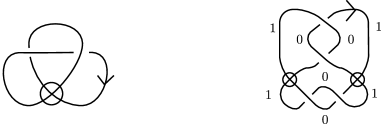
(i)                                       (ii)

Figure 7. (i) A diagram which does not admit an Alexander numbering and (ii) a diagram which does

Figure 8 shows a mod $3$ Alexander numbering, which is not an Alexander numbering.

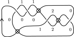
Figure 8. A mod $3$ Alexander numbering of a virtual knot diagram

A virtual link diagram is almost classical (or mod $m$ almost classical) if it admits an Alexander numbering (or a mod $m$ Alexander numbering). A virtual link $L$ is almost classical (or mod $m$ almost classical) if there is an almost classical (or mod $m$ almost classical) virtual link diagram representing $L$.

Boden, Gaudreau, Harper, Nicas and White [2] studied mod $m$ almost classical virtual knots. It is shown in [2] that for a mod $m$ almost classical virtual knot $K$, if $D$ is a minimal (in numbers of classical crossings) virtual knot diagram of $K$, then $D$ is mod $m$ almost classical.

An oriented cut point is a point on a semi-arc of $D$ at which a local orientation of the semi-arc is given ([16]). In this paper we denote it by a small triangle on the semi-arc as in Figure 9. An oriented cut point is called coherent (or. incoherent) if the local orientation indicated by the cut point is the same with (or the opposite to) the orientation of the virtual link diagram $D$.

Figure 9. An oriented cut point

Let $D$ be a virtual link diagram. A finite set of oriented cut points of $D$ is called an oriented cut system or simply a cut system if $D$ admits an Alexander numbering such that at each oriented cut point, the number increases by one in the direction of the oriented cut point (Figure 10). Such an Alexander numbering is called an Alexander numbering of a virtual link diagram with a cut system. See Figure 11 for examples.

             

Figure 10. Alexander numbering of a virtual link diagram with a cut system

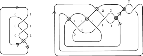
Figure 11. Alexander numberings of virtual knot diagrams with cut systems

Every virtual link diagram admits a cut system. For example, we can construct a cut system for a given virtual link diagram as below:

Example 11.

(1) The binary cut system is a cut system which is obtained by giving two oriented cut points as in Figure 12 around each classical crossing.

Figure 12. The binary cut system

The binary cut system is a cut system, since we have an Alexander numbering using only $0$ and $1$ as in Figure 13 for each crossing.

Figure 13. The binary cut system with an Alexander numbering

(2) The flat cut system of $D$ is a cut system which is obtained by giving two oriented cut points as in Figure 14 around each virtual crossing.

Figure 14. The flat cut system

The flat cut system is a cut system: Consider a collection of embedded oriented loops in $\mathbb{R}^{2}$ obtained from $D$ by smoothing at all (classical/virtual) crossings. We can assign integers to the loops such that an Alexander numbering of $D$ is induced from the integers. See Figure 15 for a local picture around each crossing.

Figure 15. The flat cut system with an Alexander numbering

The local transformations of oriented cut points depicted in Figure 16 are called oriented cut point moves. For a virtual link diagram with a cut system, the result by an oriented cut point move is also a cut system of the same virtual link diagram. Note that the move III^′ depicted in Figure 16 is obtained from the move III modulo the moves II.

I II III III^′

Figure 16. Oriented cut point moves

Theorem 12 ([16]).

Two cut systems of the same virtual link diagram are related by a finite sequence of oriented cut point moves.

Corollary 13 ([16]).

Let $D$ be a virtual link diagram and $C$ a cut system of $D$. The number of coherent cut points of $C$ equals that of incoherent cut points of $C$.

Proof.

The binary cut system for $D$ has the property that the number of coherent cut points equals that of incoherent cut points. Since each oriented cut point move preserves this property, by Theorem 12 we see that any cut system has the property. $\square$

Let $D$ be a virtual link diagram and $C$ a cut system of $D$. Let $c$ be a classical self-crossing of $D$ and let $D_{c}$ be the virtual link diagram obtained from $D$ by smoothing at $c$. Let $D_{c}^{\rm O}$ and $D_{c}^{\rm U}$ be the over and under counting components for $D$ at $c$.

For $\ast\in\{{\rm O},{\rm U}\}$, let $\rho^{\ast}(c,C)$ be the number of incoherent cut points of $C$ appearing on $D_{c}^{\ast}$ minus that of coherent ones.

Lemma 14.

Let $C$ and $C^{\prime}$ be cut systems of $D$. Let $\ast\in\{{\rm O},{\rm U}\}$. Then $\rho^{\ast}(c,C)=\rho^{\ast}(c,C^{\prime})$ for $c\in{\rm Self}X(D)$.

Proof.

We show that $\rho^{\ast}(c,C)$ is preserved under oriented cut point moves (Figure 16). It is obvious that $\rho^{\ast}(c,C)$ is preserved under moves I and II. Consider a move III and let $c_{1}$ be the classical crossing as in the figure. If $c\neq c_{1}$, then it is obvious that $\rho^{\ast}(c,C)$ is preserved. If $c=c_{1}$, then the number of coherent cut points on $D_{c}^{\rm O}$ (or $D_{c}^{\rm U}$) increases by one and that of incoherent cut points increases by one. Thus $\rho^{\ast}(c,C)$ is also preserved in this case. $\square$

By this lemma, for a classical self-crossing $c$ of a virtual link diagram $D$, we may define $\rho^{\ast}(c)$ by $\rho^{\ast}(c,C)$, where $\ast\in\{{\rm O},{\rm U}\}$ and $C$ is any cut system of $D$.

Lemma 15.

For a classical self-crossing $c$ of a virtual link diagram $D$, $\rho^{\ast}(c)={\rm ind}^{\ast}(c)$, where $\ast\in\{{\rm O},{\rm U}\}$.

Proof.

Let $C$ be the binary cut system of $D$. See Figure 12. Near the crossing $c$, a pair of coherent cut point and an incoherent cut point appear. They do not contribute to $\rho^{\ast}(c)$.

Let $\gamma_{1},\dots,\gamma_{k}$ be the sequence of classical crossings of $D$ appearing on $D_{c}^{\ast}$ in this order when we go along $D_{c}^{\ast}$ from a point near $c$ and come back to the point. Let $\gamma$ be one of $\gamma_{1},\dots,\gamma_{k}$.

Suppose that we go through $\gamma$ as over crossing. If ${\rm sgn}(\gamma)$ is $+1$ (or $-1$), then the oriented cut point on $D_{c}^{\ast}$ near $\gamma$ is coherent (or incoherent).

Suppose that we go through $\gamma$ as under crossing. If ${\rm sgn}(\gamma)$ is $+1$ (or $-1$), then the oriented cut point on $D_{c}^{\ast}$ near $\gamma$ is incoherent (or coherent).

Thus we have $\rho^{\ast}(c)={\rm ind}^{\ast}(c)$. $\square$

Definition 16.

Let $D$ be a virtual link diagram. Let $n$ be a non-zero integer.

• The over $n$-cut-writhe of $D$ is defined by

  $$J^{\prime\rm O}_{n}(D)=\sum_{c\in{\rm Self}X(D)~{}:~{}\rho^{\rm O}(c)=n,~{}\rho^{\rm U}(c)\neq 0}{\rm sgn}(c).$$

• The under $n$-cut-writhe of $D$ is defined by

  $$J^{\prime\rm U}_{n}(D)=\sum_{c\in{\rm Self}X(D)~{}:~{}\rho^{\rm U}(c)=n,~{}\rho^{\rm O}(c)\neq 0}{\rm sgn}(c).$$

• The over affine cut-index polynomial of $D$ is defined by

  $$P^{\prime\rm O}_{D}(t)=\sum_{c\in{\rm Self}X(D)~{}:~{}\rho^{\rm U}(c)\neq 0}{\rm sgn}(c)(t^{\rho^{\rm O}(c)}-1).$$

• The under affine cut-index polynomial of $D$ is defined by

  $$P^{\prime\rm U}_{D}(t)=\sum_{c\in{\rm Self}X(D)~{}:~{}\rho^{\rm O}(c)\neq 0}{\rm sgn}(c)(t^{\rho^{\rm U}(c)}-1).$$

• The over-under cut-affine index polynomial of $D$ is defined by

  $$P^{\prime\rm OU}_{D}(s,t)=\sum_{c\in{\rm Self}X(D)}{\rm sgn}(c)(s^{\rho^{\rm O}(c)}-1)(t^{\rho^{\rm U}(c)}-1).$$

Then by Lemma 15 we have the following.

Theorem 17.

Let $D$ be a virtual link diagram. Then $J^{\ast}_{n}(D)=J^{\prime\ast}_{n}(D)$ $(n\neq 0)$ and $P^{\ast}_{D}(t)=P^{\prime\ast}_{D}(t)$ for $\ast\in\{{\rm O},{\rm U}\}$, and $P^{\prime\rm OU}_{D}(s,t)=P^{\prime\rm OU}_{D}(s,t)$.

Definition 16 does not introduce new invariants, but it gives an alternative definition or a method of computing the invariants defined in Definition 6 by using cut systems. When a virtual link diagram is given with a cut system, we can compute the invariants somehow easier than using the original definition.

Now we consider the case of a virtual knot.

For a classical crossing $c$ of a virtual knot diagram $D$, we define $\rho(c)$ or $\rho(c,D)$ by $\rho^{\rm O}(c)$. Note that $\rho^{\rm U}(c)=-\rho^{\rm O}(c)$, since ${\rm ind}^{\rm U}(c)=-{\rm ind}^{\rm O}(c)$.

Definition 18.

For each non-zero integer $n$, we define the $n$-cut-writhe of $D$, denoted by $J^{\prime}_{n}(D)$, by

$$J^{\prime}_{n}(D)=\sum_{c\in X(D)~{}:~{}\rho(c)=n}{\rm sgn}(c).$$

By definition, for a virtual knot diagram $D$, $J^{\prime}_{n}(D)=J^{\prime\rm O}_{n}(D)$. By Lemma 15 (or Theorem 17), we have the following.

Theorem 19.

Let $n$ be a non-zero integer. For any virtual knot diagram $D$, $J^{\prime}_{n}(D)=J_{n}(D)$. In particular, the $n$-cut-writhe is a virtual knot invariant.

Again, we note that the $n$-cut-writhe $J^{\prime}_{n}(D)$ is nothing more than the $n$-writhe $J_{n}(D)$. However, when a virtual knot diagram is given with a cut system, it gives an alternative method of computing the $n$-writhe.

Example 20.

Let $K$ be a virtual knot represented by a diagram depicted in Figure 17 (left), which is mod $3$ almost classical. It has a cut system as in the figure (right). Let $c_{1},c_{2},c_{3}$ and $c_{4}$ be the classical crossings of the diagram from the top. Then $\rho(c_{1})=3$, $\rho(c_{2})=-3$, $\rho(c_{3})=0$ and $\rho(c_{4})=0$. Thus, we have $J_{3}(K)=J^{\prime}_{3}(D)=1$, $J_{-3}(K)=J^{\prime}_{-3}(D)=1$ and $J_{n}(K)=J^{\prime}_{n}(D)=0$ for any non-zero integer $n$ with $n\neq\pm 3$.

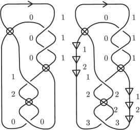
Figure 17. A mod $3$ almost classical virtual knot diagram (left) and a cut system of it (right)

Proposition 21.

Let $K$ be an almost classical virtual knot. Then we have $J_{n}(K)=0$ for any non-zero integer $n$.

Proof.

Let $D$ be an almost classical virtual knot diagram representing $K$. Since $D$ has an empty cut system, $\rho(c)=0$ for $c\in X(D)$ and hence $J_{n}(K)=J_{n}(D)=J^{\prime}_{n}(D)=0$. $\square$

For example, the virtual knot diagram depicted in Figure 7 (ii) is almost classical. Thus $\rho(c)=0$ for $c\in X(D)$ and hence the $n$-writhe is zero for $n\neq 0$.

Proposition 22.

Let $K$ be a mod $m$ almost classical virtual knot. Then we have $J_{n}(K)=0$ unless $n\equiv 0\pmod{m}$.

Proof.

Let $D$ be a mod $m$ almost classical virtual knot diagram representing $K$. Then $\rho(c)\equiv 0\pmod{m}$ for any $c\in X(D)$, which implies that $J^{\prime}_{n}(D)=0$ unless $n\equiv 0\pmod{m}$. Thus $J_{n}(K)=J_{n}(D)=J^{\prime}_{n}(D)=0$ unless $n\equiv 0\pmod{m}$. $\square$

For example, let $K$ be a virtual knot represented by the diagram $D$ depicted in Figure 17. Since $J_{3}(D)=1$, we see that the virtual knot $K$ is not mod $m$ almost classical unless $m=3$ or $m=1$.

6. Twisted knots and links

A twisted knot (or link) diagram is a virtual knot (or link) diagram possibly with some bars on its arcs. In Figure 18, three twisted knot diagrams are depicted. Twisted moves are local moves depicted in Figure 19.

$D_{1}$ $D_{2}$ $D_{3}$ (i) (ii) (iii)

Figure 18. Example of twisted knot diagrams

I II III

Figure 19. Twisted moves

Two twisted knot (or link) diagrams $D$ and $D^{\prime}$ are said to be equivalent if they are related by a finite sequence of generalized Reidemeister moves (Figure 1), twisted moves (Figure 19) and isotopies of $\mathbb{R}^{2}$. A twisted knot (or link) is an equivalence class of twisted knot (or link) diagrams.

By definition, if two classical link diagrams are equivalent as classical links then they are equivalent as virtual links. If two virtual link diagrams are equivalent as virtual links then they are equivalent as twisted links. Thus we have two maps,

$$\Phi:\{\text{\rm classical links}\}\to\{\text{\rm virtual links}\}\quad\text{\rm and}\quad\Psi:\{\text{\rm virtual links}\}\to\{\text{\rm twisted links}\}.$$

It is know that $\Phi$ is injective ([9]) and so is $\Psi\circ\Phi:\{\text{\rm classical links}\}\to\{\text{\rm twisted links}\}$ ([1, 19]). Thus, virtual links and twisted links are generalizations of classical links. The map $\Psi$ is not injective. However, it is understood well when two virtual links are equivalent as twisted links ([19]).

In [18], a method of constructing a virtual link diagram called a double covering diagram from a given twisted link diagram is introduced.

Theorem 23 ([18]).

Let $D$ and $D^{\prime}$ be twisted link diagrams and let $\widetilde{D}$ and $\widetilde{D^{\prime}}$ be their double covering diagrams. If $D$ and $D^{\prime}$ represent the same twisted link, then $\widetilde{D}$ and $\widetilde{D^{\prime}}$ represent the same virtual link.

The double cover or the double covering virtual link of a twisted link $L$, denoted by $\widetilde{L}$, is defined as the virtual link represented by a double covering diagram of a diagram of $L$.

Using the theorem, for a virtual link invariant $f$ we can obtain a twisted link invariant $\tilde{f}$ by

$$\tilde{f}(D)=f(\widetilde{D})\quad\text{\rm or}\quad\tilde{f}(L)=f(\widetilde{L})$$

for a twisted link diagram $D$ or a twisted link $L$, where $\widetilde{D}$ is a double covering diagram of $D$ and $\widetilde{L}$ is the double covering virtual link of $L$.

Definition 24.

For a twisted link diagram $D$, we define $\widetilde{J}^{\ast}_{n}(D)$, $\widetilde{P}^{\ast}_{D}(t)$ $(\ast\in\{{\rm O},{\rm U}\})$ and $\widetilde{P}^{\rm OU}_{L}(s,t)$ to be $J^{\ast}_{n}(\widetilde{D})$, $P^{\ast}_{\widetilde{D}}(t)$ and $P^{\rm OU}_{\widetilde{D}}(s,t)$, respectively, where $\widetilde{D}$ is a double covering diagram of $D$.

By Theorem 23, these are invariants of twisted links.

When $D$ is a twisted knot diagram, by construction, the double covering diagram $\widetilde{D}$ is a virtual knot diagram or a $2$-component virtual link diagram. We say that $D$ is of odd type (or even type) if $\widetilde{D}$ is a virtual knot diagram (or a $2$-component virtual link diagram). A twisted knot diagram is of odd type (or even type) if and only if the number of bars on $D$ is odd (or even).

For a virtual knot invariant $f$, we can obtain an invariant $\tilde{f}$ of a twisted knot of odd type by

$$\tilde{f}(D)=f(\widetilde{D})\quad\text{\rm or}\quad\tilde{f}(K)=f(\widetilde{K})$$

for a twisted knot diagram $D$ or a twisted knot $K$ of odd type, where $\widetilde{D}$ is a double covering diagram of $D$ and $\widetilde{K}$ is the double covering virtual knot of $K$.

Definition 25.

For a twisted knot diagram $D$ of odd type, we define $\widetilde{J}_{n}(D)$ $(n\neq 0)$ and $\widetilde{P}_{D}(t)$ to be $J_{n}(\widetilde{D})$ and $P_{\widetilde{D}}(t)$, respectively, where $\widetilde{D}$ is a double covering diagram of $D$.

By Theorem 23, these are invariants of twisted knots of odd type.

7. An invariant of twisted knots and links

In this section, we introduce a new twisted link invariant using over and under affine indices ${\rm ind}^{\rm O}(c)$ and ${\rm ind}^{\rm U}(c)$ modulo $2$.

Let $D$ be a twisted link diagram and ${\rm Self}X(D)$ be the set of classical self-crossings of $D$. Let $c\in{\rm Self}X(D)$ and let $D_{c}$ be the twisted link diagram obtained from $D$ by smoothing at $c$. The over counting component $D_{c}^{\rm O}$ and the under counting component $D_{c}^{\rm U}$ for $D$ at $c$ are defined as in Figure 3 or 4.

For $\ast\in\{{\rm O},{\rm U}\}$, let $\bar{\rho}^{\ast}(c)$ be $1$ (or $0$) if ${\rm ind}^{\ast}(c)$ is odd (or even). Here we assume that ${\rm ind}^{\ast}(c)$ $(\ast\in\{{\rm O},{\rm U}\})$ is defined as before by ignoring bars appearing on the counting component $D_{c}^{\ast}$.

For $\ast\in\{{\rm O},{\rm U}\}$, let $p^{\ast}(c)$ be $1$ (or $0$) if the number of bars on $D_{c}^{\rm O}$ is odd (or even).

Definition 26.

For a twisted virtual link diagram $D$, we define a polynomial $Q_{D}(s,t)$ by

$$Q_{D}(s,t)=\sum_{c\in{\rm Self}X(D)}{\rm sgn}(c)(s^{\bar{\rho}^{\rm O}(c)}t^{p^{\rm O}(c)}-1)(s^{\bar{\rho}^{\rm U}(c)}t^{p^{\rm U}(c)}-1).$$

Theorem 27.

The polynomial $Q_{D}(s,t)$ is an invariant of a twisted link.

Proof.

Virtual Reidemeister moves do not change $Q_{D}(s,t)$. Thus, it is sufficient to show that $Q_{D}(s,t)$ is preserved under Reidemeister moves and twisted moves.

(i) Let $D^{\prime}$ be obtained from $D$ by a Reidemesiter move I as in Figure 1, where we assume $X(D^{\prime})=X(D)\cup\{c_{1}\}$. For $c\in X(D)=X(D^{\prime})\setminus\{c_{1}\}$, we see that $\bar{\rho}^{\ast}(c)$ and $p^{\ast}(c)$ $(\ast\in\{{\rm O},{\rm U}\})$ do not change. Since $\bar{\rho}^{\ast}(c_{1})=0$ and $p^{\ast}(c_{1})=0$ for at least one $\ast\in\{{\rm O},{\rm U}\}$, we have $Q_{D}(s,t)=Q_{D^{\prime}}D(s,t)$.

(ii) Let $D^{\prime}$ be obtained from $D$ by a Reidemesiter move II as in Figure 1. For $c\in X(D)=X(D^{\prime})\setminus\{c_{1},c_{2}\}$, we see that $\bar{\rho}^{\ast}(c)$ and $p^{\ast}(c)$ $(\ast\in\{{\rm O},{\rm U}\})$ do not change. Note that $\bar{\rho}^{\ast}(c_{1})=\bar{\rho}^{\ast}(c_{2})$ and $p^{\ast}(c_{1})=p^{\ast}(c_{2})$. Since ${\rm sgn}(c_{1})=-{\rm sgn}(c_{2})$, we see that the contribution of $c_{1}$ cancels with that of $c_{2}$.

(iii) Let $D^{\prime}$ be obtained from $D$ by a Reidemesiter move III as in Figure 1. For $c\in X(D)\setminus\{c_{1},c_{2},c_{3}\}=X(D^{\prime})\setminus\{c^{\prime}_{1},c^{\prime}_{2},c^{\prime}_{3}\}$, we see that $\bar{\rho}^{\ast}(c)$ and $p^{\ast}(c)$ $(\ast\in\{{\rm O},{\rm U}\})$ do not change. Note that, for $i\in\{1,2,3\}$, ${\rm sgn}(c_{i})={\rm sgn}(c^{\prime}_{i})$ and for $\ast\in\{{\rm O},{\rm U}\}$, $\bar{\rho}^{\ast}(c_{i})=\bar{\rho}^{\ast}(c^{\prime}_{i})$ and $p^{\ast}(c_{i})=p^{\ast}(c^{\prime}_{i})$. Thus we have $Q_{D}(s,t)=Q_{D^{\prime}}D(s,t)$.

(iv) Let $D^{\prime}$ be obtained from $D$ by a twisted move I or II. In this case it is obvious that $Q_{D}(s,t)=Q_{D^{\prime}}D(s,t)$.

(v) Let $D^{\prime}$ be obtained from $D$ by a twisted move III as in Figure 19. For $c\in X(D)\setminus\{c_{1}\}=X(D^{\prime})\setminus\{c^{\prime}_{1}\}$, we see that $\bar{\rho}^{\ast}(c)$ and $p^{\ast}(c)$ $(\ast\in\{{\rm O},{\rm U}\})$ do not change. Note that $D_{c_{1}}^{\rm O}={D^{\prime}}_{c^{\prime}_{1}}^{\rm U}$ and $D_{c_{1}}^{\rm U}={D^{\prime}}_{c^{\prime}_{1}}^{\rm O}$ outside of the region where the move III is applied. Then we see that

$$\bar{\rho}^{\rm O}(c_{1})=\bar{\rho}^{\rm U}(c^{\prime}_{1}),\quad p^{\rm O}(c_{1})=p^{\rm U}(c^{\prime}_{1})\quad\text{\rm and}\quad\bar{\rho}^{\rm U}(c_{1})=\bar{\rho}^{\rm O}(c^{\prime}_{1}),\quad p^{\rm U}(c_{1})=p^{\rm O}(c^{\prime}_{1}).$$

Since ${\rm sgn}(c_{1})={\rm sgn}(c^{\prime}_{1})$, we have $Q_{D}(s,t)=Q_{D^{\prime}}D(s,t)$.

Thus we see that $Q_{D}(s,t)$ is an invariant of a twisted link. $\square$

When $D$ is a twisted knot diagram, $\bar{\rho}^{\rm O}(c)=\bar{\rho}^{\rm U}(c)$. Hence we may compute one of $\bar{\rho}^{\rm O}(c)$ and $\bar{\rho}^{\rm U}(c)$ for each $c\in{\rm Self}X(D)$.

Example 28.

For the twisted knot diagram $D_{1}$ depicted in Figure 18 (i), we have $Q_{D_{1}}(s,t)=(t-1)^{2}$. It implies that $D_{1}$ is not equivalent to the unknot. In [13], the first author introduced a polynomial invariant which is similar to $Q_{D}(s,t)$. But the invariant is not the same with ours in this paper. The invariant defined in [13] does not distinguish $D_{1}$ and the unknot.

In [12] three kinds of index polynomials $\psi$, $\psi_{+1}$ and $\psi_{-1}$ are defined for a twisted link. The invariants in [12] can also distinguish $D_{1}$ and the unknot.

Example 29.

For the twisted knot diagrams $D_{2}$ and $D_{3}$ in Figure 18, we have $Q_{D_{2}}(s,t)=0$ and $Q_{D_{3}}(s,t)=-2(st-1)(s-1)$. So the invariant $Q_{D}(s,t)$ can distinguish $D_{2}$ and $D_{3}$. Since $D_{2}$ and $D_{3}$ are of odd type, we can define $\widetilde{J}_{n}(D)$ $(n\neq 0)$ for $D=D_{2}$ and $D_{3}$, which is an invariant of a twisted knot defined in Definition 25. The $n$-writhes $\widetilde{J}_{n}(D)$ $(n\neq 0)$ do not distinguish $D_{2}$ and $D_{3}$.

References

- [1] M. O. Bourgoin, Twisted link theory, Algebr. Geom. Topol. 8 (2008), no. 3, 1249–1279.
- [2] H. Boden, R. Gaudreau, E. Harper, A. Nicas, L. White, Virtual knot groups and almost classical knots, Fund. Math. 238 (2017), no.2, 101–142.
- [3] J. S. Carter, S. Kamada and M. Saito, Stable equivalence of knots on surfaces and virtual knot cobordisms, J. Knot Theory Ramifications 11 (2002), no. 3, 311–322.
- [4] Z. Cheng, A polynomial invariant of virtual knots, Proc. Amer. Math. Soc. 142 (2014), no. 2, 713–725.
- [5] Z. Cheng and H. Gao, A polynomial invariant of virtual links, J. Knot Theory Ramifications 22 (2013), no. 22, 1341002 (33 pages).
- [6] H. A. Dye, Cut points: an invariant of virtual links, J. Knot Theory Ramifications 26 (2017), no. 9, 1743006 (10 pages).
- [7] H. A. Dye, Checkerboard framings and states of virtual link diagrams, in ”Knots, links, spatial graphs, and algebraic invariants”, pp. 53–64, Contemp. Math., 689, Amer. Math. Soc., Providence, RI, 2017.
- [8] L. C. Folwaczny and L. H. Kauffman, A linking number definition of the affine index polynomial and applications, arXiv:1211.1747, 2012.
- [9] M. Goussarov, M. Polyak and O. Viro, Finite-type invariants of classical and virtual knots, Topology 39 (2000), no. 5, 1045–1068.
- [10] A. Henrich, A sequence of degree one Vassiliev invariants for virtual knots, J. Knot Theory Ramifications 19 (2010), no.4, 461–487.
- [11] Y. H. Im, K. Lee and Y. Lee, Index polynomial invariant of virtual links, J. Knot Theory Ramifications 19 (2010), no. 5, 709–725.
- [12] H. Ito and S. Kamada, Twisted intersection colorings, invariants and double coverings of twisted links, Internat. J. Math. 34 (2023), no. 6, 2350032 (20 pages).
- [13] N. Kamada, Index polynomial invariant of twisted links, J. Knot Theory Ramifications 22 (2013), no. 4, 1340005 (16pages)
- [14] N. Kamada, Converting virtual link diagrams to normal ones, Topology Appl. 230 (2017), 161–171.
- [15] N. Kamada, Coherent double coverings of virtual link diagrams, J. Knot Theory Ramifications 27 (2018), no. 11, 1843004 (18 pages).
- [16] N. Kamada, Cyclic covering of virtual link diagrams, Internat. J. Math. 30 (2019), no. 14, 1950072 (16 pages).
- [17] N. Kamada and S. Kamada, Abstract link diagrams and virtual knots, J. Knot Theory Ramifications 9 (2000), no.1, 93–106.
- [18] N. Kamada and S. Kamada, Double coverings of twisted links, J. Knot Theory Ramifications 25 (2016), no. 9, 1641011 (22 pages).
- [19] N. Kamada and S. Kamada, Virtual links which are equivalent as twisted links, Proc. Amer. Math. Soc. 148 (2020), no.5, 2273–2285.
- [20] L. H. Kauffman, Virtual knot theory, European J. Combin. 20 (1999), no. 7, 663–690.
- [21] L. H. Kauffman, A self-linking invariant of virtual knots, Fund. Math. 184 (2004), 135–158.
- [22] L. H. Kauffman, An affine index polynomial invariant of virtual knots, J. Knot Theory Ramifications 22 (2013), No.4, 134007 (30 pages).
- [23] L. H. Kauffman, Virtual knot cobordism and the affine index polynomial J. Knot Theory Ramifications 27 (2018), no. 11, 1843017 (29 pages).
- [24] N. Petit, The multi-variable affine index polynomial, Topology Appl. 274 (2020), 107145 (15 pages).
- [25] S. Satoh and K. Taniguchi, The writhe of a virtual knot, Fundamenta Mathematicae 225 (2014), no. 1, 327–341.