Dephasing due to electromagnetic interactions in spatial qubits

Abstract

Matter-wave interferometers with micro-particles will enable the next generation of quantum sensors capable of probing minute quantum phase information. Therefore, estimating the loss of coherence as well as the degree of entanglement degradation for such interferometers is essential. In this paper we will provide a noise analysis in frequency-space focusing on electromagnetic sources of dephasing. We will assume that our matter-wave interferometer has a residual charge or dipole which can interact with a neighbouring particle in the ambience. We will investigate the dephasing due to the Coulomb, charge-induced dipole, charge-permanent dipole, and dipole-dipole interactions. All these interactions constitute electromagnetically driven dephasing channels that can affect single or multiple interferometers. As an example, we will apply the obtained formuale to situations with two adjacent micro-particles which can provide insight for the noise analysis in the quantum gravity-induced entanglement of masses (QGEM) protocol and the C-NOT gate.

I Introduction

One of the key features of quantum mechanics is the matter-wave duality exhibited in interferometery with massive systems de1923waves . Matter-wave interferometry has played a central role in many experimental breakthroughs in quantum mechanics thomson1927diffraction ; davisson1927diffraction ; davisson1928reflection , and also illustrates the idea of the spatial quantum superposition Schrodinger:1935zz . Matter-wave interferometry has been used to detect the Earth’s gravitationally-induced phase in a series of seminal experiments with neutrons and atoms colella1975observation ; nesvizhevsky2002quantum ; fixler2007atom ; asenbaum2017phase ; overstreet2022observation . Moreover, it has been suggested as a tool for sensing gravitational waves Marshman:2018upe , neutrinos Kilian:2022kgm , and as a probe for physics beyond the standard model Barker:2022mdz .

When two or more interferometers can be placed adjacent to each other they can also test the quantum entanglement feature einstein1935can ; bell1964einstein ; Horodecki:2009zz . Recently, it has been suggested that matter-wave interferometery with micro-particles will be sensitive enough to probe the quantum gravity-induced entanglement of masses (QGEM) Bose:2017nin ; ICTS , see also Marletto:2017kzi . The entanglement between two adjacent matter-wave interferometers will be observed if gravity is a quantum mechanical entity, while no entanglement will be generated if gravity is inherently classical as formalized by the local operations and classical communication (LOCC) theorem  Bennett:1996gf ; Bose:2017nin ; Marshman:2019sne ; Bose:2022uxe . Such entangled pairs also provide the basis for a quantum computer as they form the controlled-NOT (CNOT) gate, or more generally the Molmer-Sorensen gate in the context of an ion trap Soerensen:1998mp . One can go one step further and test the quantum light bending interaction Biswas:2022qto , the quantum version of the equivalence principle Bose:2022czr ; Chakraborty:2023kel , test for massive graviton Elahi:2023ozf , non-local aspects of quantum gravity Vinckers:2023grv , and verify the quantum nature of gravity in the process of measurement Hanif:2023fto .

Given so many applications on the horizon of the next generation of matter-wave interferometers, it is essential to understand various causes of decoherence and dephasing. Large spatial quantum superpositions vandeKamp:2020rqh ; PhysRevLett.111.180403 ; PhysRevLett.117.143003 ; Margalit:2020qcy ; Marshman:2021wyk ; Folman2013 ; folman2019 ; Folman2018 ; Zhou:2022frl ; Zhou:2022jug ; Zhou:2022epb ; Marshman:2023nkh have to remain coherent for the duration of the experiment in order to extract their delicate experimental signature Schut:2021svd ; Tilly:2021qef ; PhysRevLett.125.023602 ; Rijavec:2020qxd ; RomeroIsart2011LargeQS ; Chang_2009 ; Schlosshauer:2014pgr ; bassi2013models ; Toros:2020krn ; Fragolino:2023agd . Here we will focus on electromagnetic sources of dephasing induced by ambient particles located in the vicinity of the interferometeric setup.

First, we will consider a single matter-wave interferometer. We will investigate the acceleration noise caused by a single particle passing by the interferometer and estimate how it will dephase the matter-wave interferometer via electromagnetic interactions. Then, we will consider if two such entangled interferometers were kept adjacent; the source of acceleration noise will also contribute to entanglement degradation. If the matter-wave interferometer consists of a neutral micro-particle then the dominant contribution to the acceleration results from its dipole (either permanent of induced). If the micro-particle possesses any residual charge, such a charged interferometer can interact with an ambient charged particle or an ambient neutral particle posessing a dipole (either permanent of induced). The common aspect of all these interactions is that the moving particle will always create a slight jitter in the paths of the interferometer introducing noise and thus dephasing. We will analyse these cases systematically and quantify the resulting loss of coherence for each scenario.

To analyze the electromagnetic acceleration noise and dephasing we will employ the frequency space techniques that are commonly used to investigate Newtonian noise Saulson:1984 . The reason is that both the Coulomb and Newtonian interactions are long-range and provide a $1/r$ potential resulting in an infinite total cross section unless a cutoff for small scattering angles is applied griffiths_introduction_2018 . Since the computations of the decoherence rate based on the scattering theory generally depend on the total cross-section, see Schlosshauer:2014pgr ; Schlosshauer:2019ewh , at least for long-range interactions we have to use an alternative methodology. In this paper, we will thus adapt the frequency space methodology developed to investigate non-inertial and gravity gradient noise from Toros:2020dbf ; Wu:2022rdv to the case of electomagnetic interactions.

We will begin the paper with a generic discussion on relative acceleration noise (Sec. II), which we will then apply to electromagnetic noise sources. We will discuss separately the case of a charged and a neutral interferometer (Sec. III). First, the interaction between the charged interferometer and an external charge (Coulomb interaction), and the interaction between the charged interferometer and an induced or permanent external dipole (charge-dipole interaction) (Sec. IV). Second, we will analyze the neutral interferometer particle with a permanent or induced dipole that interacts with an external charge (dipole-charge interaction) or with an external dipole (dipole-dipole interaction) (Sec. V).

II Relative Acceleration Noise

This section will introduce the main tools to describe the relative acceleration noise (RAN) in frequency space. We will further discuss how to compute the resulting dephasing from the associated phase noise. In a nutshell, any movement of charges or dipoles in the vicinity of the matter-wave interferometer will cause a tiny jitter/acceleration noise, which we denote here by $a_{\text{noise, EM}}$, which will induce phase fluctuations and hence dephasing. The subscript EM denotes electromagnetic-type external interactions.

We will assume that the spatial superposition state can be created via the Stern-Gerlach (SG) setup as it happens in the case of spin-embedded systems with a nitrogen-vacancy (NV). We can envisage a spin-magnetic field interaction responsible for creating the superposition, e.g. using an SG apparatus, similar to what has been applied to the atomic case Folman2013 ; folman2019 ; Margalit:2020qcy ; Keil2021 ; Amit_2019 , and charged case Henkel_2019 . The other possibility will be to create a spatial superposition in an ion trap Wineland:1992 ; Wineland:1995 ; kielpinski2001recent . In either case, the matter-wave interferometer will be considered a spatial qubit, where interactions with an environment can induce a relative phase between the interferometer’s two arms (or the spatial superposition states of the spatial qubit).

II.1 General noise analysis

The difference in the phase picked up between the two arms of an interferometer is determined by the difference of the actions of the two trajectories. Taking the superposition to be along one dimension, e.g., in the $\hat{x}$-direction, without any loss of generality, it follows that the difference in phase-shift is given by Storey:1994oka :

$$\delta\phi =\phi_{R}-\phi_{L}$$ (1)

$$=\frac{1}{\hbar}\int_{t_{i}}^{t_{f}}L_{R}\left[x_{R},\dot{x_{R}}\right]-L_{L}\left[x_{L},\dot{x_{L}}\right]dt,$$

where $\phi_{i}$ and $L_{i}$ are the phases and the Lagrangians for $i=L,R$, the left and the right arm of the superposition, respectively. Here we consider a single interferometer, we will consider the case of adjacent interferometers later. The bounds of the integral are equal to the time of splitting and recombination of the two trajectories to complete a one-loop interferometer. The time when the interferometer is in a spatial superposition is given by $\tau=t_{f}-t_{i}$, where $f,i$ stands for the final and the initial time of the interferometer.

Here, we consider the non-relativistic regime of a free-falling test mass split into the superposition by an acceleration, $\lambda_{j}$, in the $\hat{x}$-direction . The Lagrangian of the two arms of the interferometer (with mass $m$) can be expressed as:

$$L_{j}=\frac{1}{2}mv_{j}^{2}-m\lambda_{j}(t)x_{j}-m\,a_{\operatorname{noise,EM}}(t)x_{j}\,.$$ (2)

We wish to close the trajectories (recombine the spatial qubit into a spin qubit) such that the wavefunctions of both trajectories nearly overlap. If they do not, there will be a substantial loss of visibility. If the spread of the wavepackets is $\sigma$ then one would require $|X_{L}(t_{f})-X_{R}(t_{f})|\ll\sigma$ to achieve the required visibility Schwinger ; Scully ; Englert .

The noise we will consider in the trajectories can be modelled by the fluctuations in the phase, given by the last term in Eq. (2). We assume that $a_{\rm{noise,EM}}$ is independent of the force responsible for creating the superposition, but that it is time-dependent during $\tau=t_{f}-t_{i}$. Hence, the fluctuation in the phase shift due to the EM interaction will be given by:

$$\delta\phi=\frac{m}{\hbar}\int_{t_{i}}^{t_{f}}a_{\operatorname{noise,EM}}(t)\left(x_{R}-x_{L}\right)dt,$$ (3)

here $\delta\phi(t)$ will be treated as a statistical quantity. The measurable noise in any experiment is the statistical average of any stochastic entity, which we will denote by $\mathbb{E}[\cdot]$. The averaging can be obtained over time using a single realization of the noise for a time-varying ergodic noise. For example, the average of a time-varying stochastic quantity $\delta\phi(t)$ can be expressed as:

$$\mathbb{E}[\delta\phi]=\frac{1}{T}\int_{0}^{T}\delta\phi(t)dt\,,$$ (4)

where $T$ is the time scale much larger than any time scale characterizing the noise itself. For simplicity of the analysis, we will assume that the interferometric time scale is much shorter than the time scale $T$, i.e. $T\gg\tau$, where $\tau$ denotes the experimental time, $\tau=t_{f}-t_{i}$. Furthermore, we will take $T$ to be the total time of experiment (comprising repeated runs of the experimental sequence, where the statistic is gathered). For concreteness, we will set $T=b/v$ such that in the total experimental time, we sufficiently well capture the experimental signature of the external EM source on the experimental statistics following Ref. Saulson:1984 .

While the average of the noise can often be assumed to be zero, the autocorrelation of the acceleration noise measured at different times, $\mathbb{E}[a_{\text{noise, EM}}(t_{1}),a_{\text{noise, EM}}(t_{2})]$, is often non-zero. It is related to the power spectrum density (PSD) of the noise, denoted by $S_{aa}(\omega)$. The definition of the PSD of the noise $a_{\text{noise, EM}}$ is

$$S_{aa}(\omega)=\lim\limits_{T\to\infty}\frac{|a_{\text{noise, EM}}(\omega)|^{2}}{T},$$ (5)

where $a_{\text{noise, EM}}(\omega)$ is the Fourier transform of $a_{\text{noise, EM}}(t)$ on the time domain $[0,T]$. According to the Wiener-Khinchin theorem, the autocorrelation function of a random process is given by the PSD of that process Wiener:1930 ; Khintchine1934 :

$$\mathbb{E}\big{[}a_{\operatorname{noise,EM}}(t_{1}) a_{\operatorname{noise,EM}}(t_{2})\big{]}$$ (6)

$$=\frac{1}{2\pi}\int_{\omega_{\rm min}}^{\infty}S_{aa}(\omega)e^{i\omega(t_{1}-t_{2})}d\omega\,,$$

where the minimum frequency $\omega_{\operatorname{min}}=2\pi/(t_{f}-t_{i})$ is the frequency resolution in the experiment . In particular, signals and noises are sampled as a discrete finite data series, so the frequency-domain analysis has to be based on the discrete Fourier transform, which has such a frequency resolution Chatfield:2016 .

Using the relation in Eq. (6) and the difference in phase-shift form Eq. (3), the variance $\mathbb{E}[(\delta\phi)^{2}]$ can be written in the Fourier space by:

$$\Gamma_{\operatorname{n}}=\mathbb{E}\left[(\delta\phi)^{2}\right]=\frac{1}{2\pi}\left(\frac{m}{\hbar}\right)^{2}\int_{\omega_{\rm min}}^{\infty}d\omega S_{\operatorname{aa}}(\omega)F(\omega)\,.$$ (9)

where $\Gamma_{\operatorname{n}}$ in Eq. (9) is the variance in the noise, which is an observable entity, and $F(\omega)$ is known as the transfer function Wu:2022rdv ; Toros:2020dbf . As shown below, $\Gamma_{\rm n}$ will be useful to estimate the dephasing for the two spatial qubits, which will add up to any other sources of decoherence caused by the extrenal/internal degrees of freedom. Note that the $\Gamma_{n}$ is a dimensionless entity.

The transfer function is equal to the absolute value squared of the Fourier transform of the difference in the trajectories:

$$F(\omega) =\left|\int_{t_{i}}^{t_{f}}dt\left(x_{L}-x_{R}\right)e^{i\omega t}\right|^{2}$$ (10)

$$=\left|-\frac{1}{\omega^{2}}\int_{t_{i}}^{t_{f}}\frac{d^{2}}{dt^{2}}\left(x_{L}-x_{R}\right)e^{i\omega t}dt\right|^{2},$$

In the second line we find the dependency on the acceleration, $\text{d}^{2}x/\text{d}t^{2}$, which as we will see can be related to particle equations of motion, and follows from integration by parts and the equality of both the position and velocity at the path’s endpoints from the first line.

II.2 Example of Stern-Gerlach interferometer

The dephasing in Eq. (9) is dependent on the specific trajectory of the two arms of the matter-wave interferometer (via the transfer function $F(\omega)$). Here, we assume an SG type interferometer that is often proposed in the context of entanglement-based quantum-gravity experiments, see Bose:2017nin ; Marshman:2019sne ; Zhou:2022jug ; Zhou:2022frl ; Zhou:2022epb ; Japha:2022xyg .

We specify the trajectory of two arms of the interferometer, see Fig. 1. Here, we assume a symmetric path for the interferometer as a prototype model. We consider a simplistic scenario, assuming that the acceleration of the spin state $j$, denoted $\lambda_{j}$, is proportional to the gradient of the magnetic field, given by:

$$\lambda_{j}=s_{j}\frac{g\mu_{B}}{m}|\nabla B|$$ (11)

where $s_{j}$ is the spin of the state, $g$ is the Lande g-factor of the electron ($g=2$), $\mu_{B}=9\cdot 10^{-24}\operatorname{J\,T}^{-1}$ is the Bohr-magneton, $m$ is the mass of the test-mass and $|\nabla B|$ is the magnitude of the gradient of the magnetic field. To create the path in Fig. 1, one controls the spin so that the acceleration of the right arms is positive from $[0,t_{a}]$ and $[3t_{a}+t_{e},4t_{a}+t_{e}]$ and negative from $[t_{a},2t_{a}]$ and $[2t_{a}+t_{e},3t_{a}+t_{e}]$, while it is zero for the time range $[2t_{a},2t_{a}+t_{e}]$. For the left arm, the spin and, hence, the acceleration will be equal in magnitude but in the opposite direction. We also assume $x_{j}(0)=0$ and $\dot{x}_{j}(0)=0$ for solving the equations of the motion for the trajectory, given by: $\ddot{x}_{j}(t)=\lambda_{j}(t)$. Micro-particles can be electrically charged by ultraviolet irradiation Frimmer_2017 . For a small number of charges $n$, the Lorentz force acting on the micro-particle $\sim nevB/m$ (with $e$ the unit of electric charge) is negligible due to its large mass $m$, see Henkel_2019 .

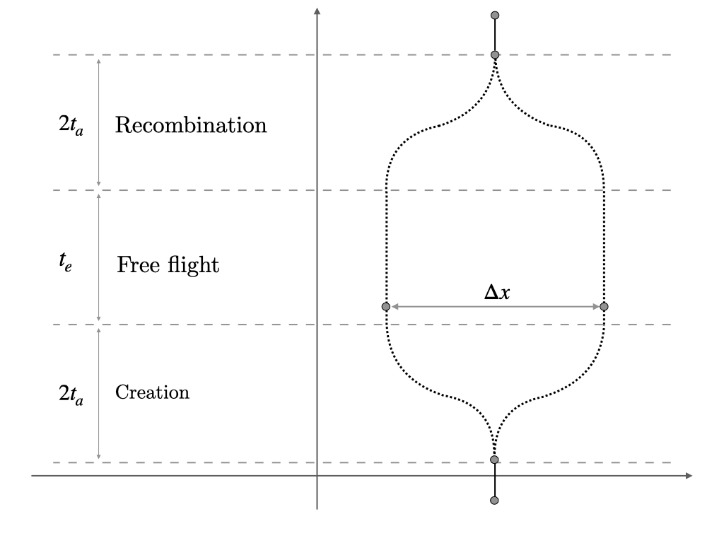
Figure 1: Schematic illustration of the paths of the arms of the interferometer (adapted from Toros:2020dbf ; Wu:2022rdv ). Based on this figure, the transfer function in Eq. (12) can be calculated. For the left arm, the acceleration is in the negative direction from $[0,t_{a}]$ and $[3t_{a}+t_{e},4t_{a}+t_{e}]$, in the positive direction from $[t_{a},2t_{a}]$ and $[2t_{a}+t_{e},3t_{a}+t_{e}]$, while it is zero for the time range $[2t_{a},2t_{a}+t_{e}]$. Meanwhile, the acceleration is the opposite for the right arm.

With the help of the equations of motion the transfer function corresponding to the trajectory illustrated in Fig. 1 can be computed:

$$F(\omega) =\frac{1}{\omega^{2}}\left|\int_{t_{i}}^{t_{f}}\left(\lambda_{L}-\lambda_{R}\right)e^{i\omega t}dt\right|^{2}=\left|\frac{2}{\omega^{2}}\int_{t_{i}}^{t_{f}}\lambda_{s}e^{i\omega t}dt\right|^{2}$$ (12)

$$=\frac{32\lambda_{s}^{2}}{\omega^{6}}\sin^{4}\left(\frac{t_{a}\omega}{2}\right)\sin^{2}\left(\frac{\omega}{2}(2t_{a}+t_{e})\right)\,.$$

Since the means by which the superposition is created is immaterial, for the calculation of the transfer function it is convenient to define the transfer function in terms of the maximal superposition size created after two acceleration times, $\Delta x=\lambda t_{a}^{2}$:

$$F(\omega)=\frac{32(\Delta x)^{2}}{\omega^{6}t_{a}^{4}}\sin^{4}\left(\frac{t_{a}\omega}{2}\right)\sin^{2}\left(\frac{\omega}{2}(2t_{a}+t_{e})\right).$$ (13)

By finding the PSD, $S_{aa}$, due to different types of interaction and combining it with the specifics of the trajectory encoded in the transfer function in Eq. (13), we can find the noise via Eq. (9).

III EM induced acceleration noise

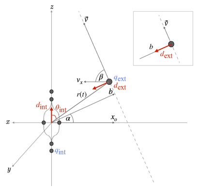
Figure 2: Illustration of the interferometer and of the external particle (i.e., the source of dephasing). The position of the closest approach is $(x_{0},y_{0},z_{0})$ corresponding to the impact parameter $b$ (the centre-of-mass of the interferometer is used for the definition since we assume $\Delta x\ll b$). The magnitude of the position vector is given by $|\bm{r}|=\sqrt{b^{2}+(vt^{2})}$, where the velocity is $v=|\bm{v}|=(v_{x},v_{y},v_{z})$. The projection angles are defined by $\cos(\alpha)=x_{0}/b$  and  $\cos(\beta)=v_{x}/v$. The dipole moments are denoted by the red arrows.

We will assume that the external particle is moving with a constant velocity $\bm{v}$ and with an impact parameter $b$ with respect to the matter-wave interferometer (see Fig. 2). The position of the external particle concerning the matter-wave interferometer can be conveniently described by the vector $\bm{r}(t)$ from the interferometer centre of mass to the external particle, with length:

$$r(t)=\sqrt{b^{2}+(vt)^{2}}.$$ (14)

The $x$-component of this vector, from the properties of the setup (see Fig. 2) is $r_{x}(t)=x_{0}+v_{x}t$. The unit vector in the $x$-direction is denoted by $\hat{\bm{r}}_{x}$, and $x_{0}$ and $v_{x}$ are defined to be the $x$-components of the impact parameter $b$ and velocity $\bm{v}$, respectively. We can thus introduce the projection angles:

$$\cos(\alpha)=x_{0}/b,\mbox{\quad\quad}\cos(\beta)=v_{x}/v.$$ (15)

The moving external particle can cause a random acceleration noise on the interferometer due to the EM interactions, contributing to a phase fluctuation of the interferometer. We also assume the micro-particle and the moving particle can be modelled as either point charges or dipoles. Specifically, we consider two cases for the interactions.

Charged interferometer: If the interferometer is charged there can be two EM interactions between the charged interferometer and the external particle:

• A charge-charge interaction between the external charge, $q_{\text{ext}}$, and the charge of the interferometer, denoted here by $q_{\text{int}}$. This interaction is given by the Coulomb potential

  $$V_{\text{cc}}(r)=\frac{1}{4\pi\epsilon_{0}}\frac{q_{\text{int}}q_{\text{ext}}}{r}\,,$$ (16)

  where both systems are considered as point charges.

• A charge-dipole interaction between the charge of the interferometer, $q_{\text{int}}$, and the dipole of the external particle, $\bm{d}_{\text{ext}}$. This interaction is given by the potential, see griffiths2013introduction ; jackson_classical_1999 :

  $$V_{\text{cd}}(r)=\frac{q_{\text{int}}}{4\pi\epsilon_{0}}\frac{\textbf{d}_{\text{ext}}\cdot\hat{\textbf{r}}}{r^{2}}\,.$$ (17)

  The external dipole can be either induced or permanent.

Neutral interferometer: If the interferometer is neutral, there can be two types of EM interactions between the interferometer and the external particle.

• A dipole-charge interaction between the dipole of the interferometer, $\bm{d}_{\text{int}}$ (which can be either permanent or induced by the EM field of the external particle), and the charge of the external particle, $q_{\text{ext}}$. This interaction is given by the potential: griffiths2013introduction

  $$V_{\text{dc}}(r)=-\frac{q_{\text{ext}}}{4\pi\epsilon_{0}}\frac{\textbf{d}_{\text{int}}\cdot\hat{\textbf{r}}}{r^{2}}\,,$$ (18)

  where the external particle is assumed to be a point charge.

• A dipole-dipole interaction, where the dipole of the interferometer, $\bm{d}_{\text{int}}$, and the dipole of the external dipole, $\bm{d}_{\text{ext}}$, are assumed to be permanent. This interaction is given by the potential: griffiths2013introduction ; jackson_classical_1999

  $$V_{\text{dd}}(r)=\frac{1}{4\pi\epsilon_{0}}\bigg{[} \frac{\textbf{d}_{\text{int}}\cdot\textbf{d}_{\text{ext}}}{r^{3}}$$

  $$\,\,-\frac{3(\textbf{d}_{\text{int}}\cdot\hat{\textbf{r}})(\textbf{d}_{\text{ext}}\cdot\hat{\textbf{r}})}{r^{3}}\bigg{]}\,,$$ (19)

  where $\hat{\bm{r}}$ is the unit vector pointing in the direction from the interferometer centre of mass to the external particle centre of mass.

These interaction potentials will cause a random noise on the interferometer $a_{\text{noise, EM}}$, which will contribute a phase fluctuation that can be detectable by sensing it if we were to use the matter-wave interferometer as a quantum sensor, or this acceleration noise will lead to dephasing the experimental outcome in a QGEM-type experiment for instance. We now give a brief outline of all the accelerations. For each of the interactions discussed above, eqs. (16)–(19), the corresponding acceleration is found via $\bm{F}=m\,\bm{a}$, with $\bm{F}=-\partial V/\partial\bm{r}$, where $m$ is the mass of the interferometer.

$$\bm{a}_{\text{cc}} =\frac{q_{\text{int}}q_{\text{ext}}}{4\pi m\epsilon_{0}}\frac{\hat{\bm{r}}(t)}{r^{2}(t)},$$ (20)

$$\bm{a}_{\text{cd}} =\frac{q_{\text{int}}}{2\pi m\epsilon_{0}}\frac{\mathbf{d}_{\text{ext}}\cdot\hat{\mathbf{r}}(t)}{r^{3}(t)}\,\hat{\bm{r}}(t)\,,$$ (21)

$$\bm{a}_{\text{dc}} =-\frac{q_{\text{ext}}}{2\pi m\epsilon_{0}}\frac{\mathbf{d}_{\text{int}}\cdot\hat{\mathbf{r}}(t)}{r^{3}(t)}\,\hat{\bm{r}}(t)\,,$$ (22)

$$\bm{a}_{\text{dd}} =\frac{3\,\hat{\bm{r}}}{4\pi\epsilon_{0}m}\left[\frac{\bm{d}_{\text{ext}}\cdot\bm{d}_{\text{int}}}{r^{4}(t)}-3\frac{(\bm{d}_{\text{ext}}\cdot\hat{\bm{r}})(\bm{d}_{\text{int}}\cdot\hat{\bm{r}})}{r^{4}(t)}\right]\,.$$ (23)

The vector $\hat{\bm{r}}$ is time-dependent and given by $\hat{\bm{r}}(t)=\bm{r}(t)/r(t)$, with $r(t)=\absolutevalue{\bm{r}(t)}$ (as defined in eq. (14)). The dipole can be either permanent or induced, which we distinguish with the notation $\bm{d}(i)$ and $\bm{d}(p)$, respectively.

Since the interferometer is created in one dimension, e.g. $\hat{x}$-direction in our case, the only relevant acceleration is in the $\hat{x}$-direction, and we are specifically interested in $a_{x}(t)$. The acceleration is found separately now for every interaction in Eqs. (16)–(19) and some assumptions are made on the orientation of the dipole vectors for simplification and to estimate the upper bound on the dephasing.

The mean value of the noise can be assumed to be zero, e.g.

$$\mathbb{E}[a_{\text{noise, EM}}]=\mathbb{E}[\delta\phi]=0\,.$$ (24)

This is because the zero point, or the baseline of the phase, can be calibrated using an axillary experiment, so the contribution of the mean value of every noise will be considered in the offset of the baseline in our current analysis. Therefore we will here focus on finding the autocorrelation of the acceleration noise at different times, $\mathbb{E}[a_{\text{noise, EM}}(t_{1}),a_{\text{noise, EM}}(t_{2})]$, see eq. (6). Taking the Fourier transform to find $a_{x}(\omega)$ on the time domain $[0,T]$, we can use eq. (5) to find the noise PSD $S(\omega)=\absolutevalue{a_{x}(\omega)}^{2}/T$. Combining the noise PSD with the transfer function gives the dephasing using eq. (9). The results for the noise are given in Sec. IV, V and the detailed calculations are given in Appendix A.

IV Charged interferometer

If there is some charge on the interferometric particle, then charge-charge interactions and charge-external dipole interactions will generate acceleration noise in the system. We consider the charge-charge interaction and the charge-dipole interaction between the interferometer and the external particle, where we investigate separately the dipole of the external particle to be permanent or induced .

IV.1 Dephasing due to internal charge and external charge interaction

First of all, we will assume the simplest case of a charged matter-wave interferometer: the matter-wave interferometer has a charge $q_{\text{int}}$, which is interacting with ambient charge $q_{\text{ext}}$ that is moving with a constant velocity and has the closest approach $b$ from the interferometer’s centre of mass. The acceleration due to the charge-charge interaction in the $\hat{x}$-direction is given by:

$$a_{x}^{\text{cc}}(t)=\frac{q_{\text{int}}q_{\text{ext}}}{4\pi\epsilon_{0}mb^{2}}\frac{\cos(\alpha)+(vt/b)\cos(\beta)}{(1+(vt/b)^{2})^{3/2}}.$$ (25)

Finding $S_{aa}$ from $a_{x}(\omega)$ and putting it in Eq. (9) yields the dephasing:

$$\Gamma_{\operatorname{n}}^{\text{cc}}=\frac{q_{\text{int}}^{2}q_{\text{ext}}^{2}(\Delta x)^{2}}{\pi^{3}\hbar^{2}\epsilon_{0}^{2}Tv^{4}t_{a}^{4}}\int_{\omega_{\operatorname{min}}}^{\infty}\omega^{-4}\operatorname{sin}^{2}\left(\frac{\omega}{2}(2t_{a}+t_{e})\right)$$ (26)

$${\operatorname{sin}}^{4}\left(\frac{t_{a}\omega}{2}\right)\left[\cos^{2}(\alpha)K_{1}^{2}\left(\frac{b\omega}{v}\right)+\cos^{2}(\beta)K_{0}^{2}\left(\frac{b\omega}{v}\right)\right]d\omega.$$

with $K_{\nu}$ is the modified Bessel function (see appendix A). The dephasing depends on the charges $q_{\text{int}}$ and $q_{\text{ext}}$, the size of the spatial superposition and the time during which it is created, the impact parameter and the velocity of the external particle. Furthermore, the time $T$ which is the time over which the phase fluctuations are averaged and the minimum frequency $\omega_{\text{min}}$ are determined by the experimental setup, impact parameter $b$ and the velocity $v$ of the external particle. The integral in eq. (26) is solved numerically, and the resulting dephasing is plotted in Sec. VI (Fig. 3(a)) for a specific interferometer scheme.

IV.2 Dephasing due to internal charge and external dipole interaction

In this section, we will consider a charged interferometer particle interacting with an external dipole. The dipole could arise due to any ambient gas particle left inside the vacuum chamber. We will only consider the acceleration noise due to one such external particle. The water vapour that can be left in the vacuum chamber consists of the water molecules which carry a permanent dipole moment. Left-over air molecules in the vacuum chamber, such as dinitrogen, carbon dioxide, argon and dioxygen are polarisable and could thus have an induced dipole moment from the charge of the interferometer. The acceleration due to the charge-dipole interaction is given in Eq. (21), and the acceleration is dependent on whether the dipole is induced or permanent.

IV.2.1 Permanent external dipole

If the external particle has a permanent dipole, such as is the case of water vapour, then the dipole moment magnitude can be taken to be the experimentally determined value, e.g. $\bm{d}_{\text{ext}}^{\text{(p)}}=6.19\times 10^{-30}\,$\mathrm{C}\text{\,}\mathrm{m}$$ in the case of water vapour (the superscript $p$ standing for permanent) lide2004crc . Taking the worst-case scenario, we assume that at the point of closest approach $b$, the dipole vector of the external particle is aligned with the vector $r(t)$. Assuming that the particle is moving very slowly, we maximize the acceleration by taking the dipole vector and the vector $\bm{r}(t)$ to align during the experimental time $\tau=t_{f}-t_{i}$. The acceleration in the $x$-direction can be found to be:

$$a_{x}^{\text{cd(p)}}(t)=\frac{q\absolutevalue{\mathbf{d}_{\text{ext}}}}{2\pi mb^{3}\epsilon_{0}}\frac{\cos(\alpha)+(vt/b)\cos(\beta)}{(1+(vt/b)^{2})^{2}}\,.$$ (27)

Its Fourier transform and the resulting PSD of the noise are given in Appendix A. The dephasing is then given by Eq. (9), the full integral will be:

$$\Gamma_{\operatorname{n}}^{\text{cd(p)}}= \frac{q^{2}|\mathbf{d}_{\operatorname{ext}}|^{2}(\Delta x)^{2}}{2\pi^{2}\hbar^{2}\epsilon_{0}^{2}Tv^{5}bt_{a}^{4}}\int_{\omega_{min}}^{\infty}\omega^{-3}\operatorname{sin}^{2}\left(\frac{\omega}{2}(2t_{a}+t_{e})\right)$$ (28)

$$\operatorname{sin}^{4}\left(\frac{t_{a}\omega}{2}\right)\Biggr{[}\cos^{2}(\alpha)K_{3/2}^{2}\left(\frac{b\omega}{v}\right)$$

$$\mbox{\quad\quad}\mbox{\quad\quad}\mbox{\quad\quad}\mbox{\quad\quad}+\cos^{2}(\beta)K_{1/2}^{2}\left(\frac{b\omega}{v}\right)\Biggr{]}d\omega\,,$$

where $K_{\nu}$ is the modified Bessel function (see appendix A). The results of the integration with the parameters of a specific interferometer setup is given in Sec. VI (Fig. 3(b)).

IV.2.2 Induced external dipole

Left-over air molecules in the vacuum chamber have a polarisability of $\alpha_{\text{pol}}\sim 10^{-40}\,$\mathrm{A}\mathrm{{}^{2}}\mathrm{s}^{4}\mathrm{/}\mathrm{k}\mathrm{g}$$ . If the dipole moment in the external particle with polarisability is induced due to the electric field $\bm{E}$ from the charged interferometer, then the result is slightly different. The induced dipole by a charge $q_{\text{int}}$ is given by:

$$\bm{d}_{\text{ext}}^{\text{(i)}}=\alpha_{\text{pol}}\bm{E}=\alpha_{\text{pol}}\frac{q_{\text{int}}}{4\pi\epsilon_{0}r^{2}}\hat{\bm{r}}\,,$$ (29)

where the superscript (i) stands for induced. The acceleration in the $\hat{x}$-direction thus becomes:

$$a_{x}^{\text{cd(i)}}(t) =\frac{q_{\text{int}}^{2}\alpha_{\text{pol}}}{8\pi^{2}mb^{5}\epsilon_{0}^{2}}\frac{\cos(\alpha)+(vt/b)\cos(\beta)}{(1+(vt/b)^{2})^{2}}\frac{1}{r^{2}(t)},$$

$$=\frac{q_{\text{int}}^{2}\alpha}{8\pi^{2}mb^{5}\epsilon_{0}^{2}}\frac{\cos(\alpha)+(vt/b)\cos(\beta)}{(1+(vt/b)^{2})^{3}}.$$ (30)

The Fourier transform and PSD are given in Appendix A. The dephasing is then found to be:

$$\Gamma_{\operatorname{n}}^{\text{cd(i)}}=\frac{q^{4}\alpha^{2}_{\text{pol}}(\Delta x)^{2}}{512\pi^{4}\hbar^{2}\epsilon_{0}^{4}v^{7}b^{3}Tt_{a}^{4}} \int_{\omega_{\operatorname{min}}}^{\infty}d\omega\frac{1}{\omega}\sin^{4}\left(\frac{t_{a}\omega}{2}\right)$$ (31)

$$\sin^{2}\left(\frac{\omega}{2}(2t_{a}+t_{e})\right) \Biggr{[}\cos^{2}(\alpha)K^{2}_{5/2}\left(\frac{b\omega}{v}\right)$$

$$+\cos^{2}(\beta)K^{2}_{3/2}\left(\frac{b\omega}{v}\right)\Biggr{]}.$$

$K_{\nu}$ is the modified Bessel function (see appendix A). Again, this expression can be solved numerically in order to obtain the dephasing. The results of the integration with the parameters of a specific interferometer setup are given in Sec. VI (figure 3(c)).

Eq. (39) differs from the permanent dipole result in Eq. (36) since the induced dipole is assumed to be induced by the interferometer charge, as a result, Eq. (39) depends on the interferometer charge and the polarisability of the external particle, $\alpha_{\text{pol}}$. The magnitude of the induced dipole is distance-dependent, resulting in a different $v,b$-dependence of Eq. (39) compared to the permanent dipole dephasing result.

V Neutral interferometer

In this section, we will assume that the micro-particles in the interferometer have a dipole $d_{\text{int}}$ (either permanent or induced) and that it is interacting with an external charged particle (of charge $q_{\text{ext}}$) or external dipole ($\bm{d}_{\text{ext}}$). We consider separately the permanent and induced dipole moments of the micro-particle in the presence of a charge.

Although the dephasing results obtained in this section are generic, we will apply them to the QGEM experiment where neutral diamond-type crystals of mass $\sim 10^{-15}\,$\mathrm{kg}$$ are considered. We briefly discuss the two different dipoles of the micro-particle in this context.

• Permanent dipole: It is possible that the microcrystal may have a permanent dipole due to the impurities on the surface or in the volume. The dipole moment of silica type material, ($\text{SiO}_{2}$), was experimentally measured in Afek:2021bua , which showed that the material exhibits no clear correlation between mass and dipole moment. That being said, the micro-particle spheres of size $10\,$\mathrm{\SIUnitSymbolMicro m}$$, $15\,$\mathrm{\SIUnitSymbolMicro m}$$ and $20\,$\mathrm{\SIUnitSymbolMicro m}$$ had permanent dipoles varying from $\sim 1000-5000\,e\,$\mathrm{\SIUnitSymbolMicro m}$$, $\sim 200-8000\,e\,$\mathrm{\SIUnitSymbolMicro m}$$ and $\sim 8500\pm 1500\,e\,$\mathrm{\SIUnitSymbolMicro m}$$ (for simplicity we use $e\,$\mathrm{\SIUnitSymbolMicro m}$$ to express the dipole, with $e$ a single electric charge such that $1\,e\,$\mathrm{\SIUnitSymbolMicro m}$\approx 1.6\times 10^{-25}\,$\mathrm{C}\text{\,}\mathrm{m}$$). This shows that there is at least an order of magnitude uncertainty in the permanent dipole magnitude. The study showed that this material’s permanent dipole moments exhibit a volume scaling, leaving the question open whether in general, the permanent dipole moment scales with the volume. For the test-mass of radius $r=0.5\,$\mathrm{\SIUnitSymbolMicro m}$$ (corresponding to $\sim 10^{-15}\,$\mathrm{kg}$$ for a spherical diamond test mass), we take the dipole moment to be $|\textbf{d}_{\text{int}}^{(p)}|\sim 0.1\,e\,$\mathrm{\SIUnitSymbolMicro m}$$, thus assuming a volume scaling, and using the experimental data in Afek:2021bua as a benchmark.

• Induced dipole: The diamond-type crystal is a dielectric material, the crystal has a polarizability $\alpha$ (in SI-units $\mathrm{A}\mathrm{{}^{2}}\mathrm{s}^{4}\mathrm{/}\mathrm{k}\mathrm{g}$). In particular, in isotropic media, a local electric field will produce a local dipole in each atom of the crystal’s lattice jackson_classical_1999 :

  $$\bm{d}_{\text{int}}^{(i)}=N\alpha_{\text{pol}}\,\bm{E}_{\text{loc}}.$$ (32)

  The local polarizability (which we denote $\alpha_{\text{pol}}$) of the atoms is related to the polarisability of the medium via the Classius-Mossotti relation:

  $$\frac{n\,\alpha_{\text{pol}}}{3\epsilon_{0}}=\frac{\epsilon_{r}-1}{\epsilon_{r}+2}\,,$$ (33)

  with $n$ the number density of atoms, $n=3N/4\pi R^{3}$ for spherical masses ($N$ the number of atoms, $R$ the radius). As a result, the dipole for a spherical diamond crystal due to an external point charge $q_{\text{ext}}$ is given by:

  $$\bm{d}_{\text{int}}^{(i)}=\frac{\epsilon_{r}-1}{\epsilon_{r}+2}\frac{q_{\text{ext}}R^{3}}{r^{2}}\hat{\bm{r}}\,,$$ (34)

  with $\epsilon_{r}$ relative permittivity of the medium.

V.1 Dephasing due to internal dipole and charge interaction

We now consider the dephasing due to an internal dipole interacting with an external charge. The acceleration was given in Eq. (22), the $x$-component of which depends on whether the dipole is permanent or induced.

V.1.1 Permanent dipole of a micro-particle

Suppose the interferometer’s micro-particle has a permanent dipole moment, similar to that of silica-type material Afek:2021bua . In that case, the dipole moment magnitude can be taken to be the experimentally determined value, e.g. $\sim e\,$\mathrm{C}\text{\,}\mathrm{m}$$ for micro-spheres, assuming a volume scaling as discussed previously. Furthermore, if we assume full control of the interferometer particle, we can take the direction of the intrinsic dipole moment to be aligned with the $\hat{z}$-axis. As detailed in Appendix A, in this scenario the component of the acceleration in the $\hat{x}$-direction is:

$$a_{x}^{\text{d(p)c}}(t)=\frac{q_{\text{ext}}|\mathbf{d}_{\text{int}}|}{2\pi mb^{3}\epsilon_{0}} \frac{\cos(\alpha)+(vt/b)\cos(\beta)}{(1+(vt/b)^{2})^{5/2}}$$ (35)

$$\bigg{[}\cos(\theta_{0})+(vt/b)\cos(\gamma)\bigg{]},$$

where $\gamma$ is the angle between the velocity vector and the $\hat{z}$-axis and $\theta_{0}$ is the angle between the vector $b$ and the $\hat{z}$-axis (the angles $\gamma$, $\theta_{0}$ are similar to the projection angles $\alpha$, $\beta$, respectively, in figure 2, but $\gamma$, $\theta_{0}$ are projection angles on the $\hat{z}$-axis rather than on the $\hat{x}$-axis, they are discussed in more detail in Appendix A).

The Fourier transform $a(\omega)$ gives an expression for the PSD, $S_{aa}(\omega)$, and from these expressions we find the dephasing parameter, see Appendix A. Taking the worst-case dephasing based on the angles $\alpha,\beta,\gamma,\theta_{0}$ (see Appendix B, where we optimise these angles to see the largest dephasing), the dephasing is given as:

$$\Gamma_{\operatorname{n}}^{\text{d(p)c}}= \frac{q_{\text{ext}}^{2}|\mathbf{d}_{\text{int}}|^{2}(\Delta x)^{2}}{9\pi^{3}\epsilon_{0}^{2}\hbar^{2}v^{6}Tt_{a}^{4}}\int^{\infty}_{\omega_{\text{min}}}\frac{1}{\omega^{2}}\sin^{4}\left(\frac{t_{a}\omega}{2}\right)$$ (36)

$$\Bigg{[}K_{2}^{2}\left(\frac{b\omega}{v}\right)+\left(2+\frac{b^{2}\omega^{2}}{v^{2}}\right)K_{1}^{2}\left(\frac{b\omega}{v}\right)$$

$$+K_{0}^{2}\left(\frac{b\omega}{v}\right)-2\frac{b\omega}{v}K_{0}\left(\frac{b\omega}{v}\right)K_{1}\left(\frac{b\omega}{v}\right)\Bigg{]}$$

$$\mbox{\quad\quad}\sin^{2}\left(\frac{\omega}{2}(2t_{a}+t_{e})\right)\differential{\omega}$$

which can be solved numerically and where $K_{\nu}$ is the modified Bessel function (see Appendix A). The results of the integration with the parameters of a specific interferometer setup are given in Sec. VI (figure 4(a)).

V.1.2 Induced dipole of a micro-particle

If the dipole is induced by the electric field of an external charge $q_{\text{ext}}$, its magnitude is given by jackson_classical_1999 ; griffiths2013introduction :

$$\bm{d}_{\text{int}}^{\text{(i)}}=\frac{\epsilon_{r}-1}{\epsilon_{r}+2}\frac{q_{\text{ext}}R^{3}}{r^{2}(t)}\hat{\bm{r}}\,,$$ (37)

with the relative permittivity of diamond $\epsilon_{r}\sim 5.7$ for diamond and $R$ the radius of the spherical diamond (the superscript (i) indicates the induced dipole). The acceleration in the $\hat{x}$-direction then becomes:

$$a_{x}^{\text{d(i)c}}(t) =\frac{\epsilon_{r}-1}{\epsilon_{r}+2}\frac{q_{\text{ext}}^{2}R^{3}}{2\pi\epsilon_{0}mb^{5}}\frac{\cos(\alpha)+(vt/b)\cos(\beta)}{(1+(vt/b)^{2})^{3}}\,.$$ (38)

The dephasing parameter is derived in detail in Appendix A, and is given by:

$$\Gamma_{\operatorname{n}}^{\text{d(i)c}}= \left(\frac{\epsilon_{r}-1}{\epsilon_{r}+2}\right)^{2}\frac{q_{\text{ext}}^{4}R^{6}(\Delta x)^{2}}{32\pi^{2}\epsilon_{0}^{2}\hbar^{2}v^{7}b^{3}Tt_{a}^{4}}\int_{\omega_{\text{min}}}^{\infty}\frac{1}{\omega}$$ (39)

$$\Biggr{[}\cos^{2}(\alpha)K^{2}_{5/2}\left(\frac{b\omega}{v}\right)+\cos^{2}(\beta)K^{2}_{3/2}\left(\frac{b\omega}{v}\right)\Biggr{]}$$

$$\mbox{\quad\quad}\sin^{4}\left(\frac{t_{a}\omega}{2}\right)\sin^{2}\left(\frac{\omega}{2}(2t_{a}+t_{e})\right)\differential{\omega},$$

and $K_{\nu}$ is the modified Bessel function (see appendix A). Again, this expression can be solved numerically to obtain the dephasing. The results of the integration with the parameters of a specific interferometer setup are given in Sec. VI (Fig. 4(b)). Eq. (39) differs from the permanent dipole result in Eq. (36) since the induced dipole is assumed to be induced by the external charge. As a result, Eq. (39) depends on the external charge and the relative permittivity and radius of the interferometer. The magnitude of the induced dipole is distance-dependent, resulting in a different $v,b$-dependence of Eq. (39) compared to the permanent dipole dephasing result of Eq. (36).

V.2 Dephasing due to internal dipole and external dipole

The acceleration from the dipole-dipole interaction was given in Eq. (23). For large $r$, we can see that the other interactions dominate this interaction since it goes as $1/r^{4}$. Sticking with the assumptions made in previous sections, that $\bm{d}_{\text{ext}}$ aligns with the $\hat{z}$-direction, and that for a short interaction time $\tau$, $\bm{d}_{\text{int}}$ approximately aligns with $\hat{\bm{r}}(t)$, the acceleration in the $\hat{x}$-direction is:

$$\bm{a}_{x}^{\text{dd}}(t)=\frac{6\absolutevalue{\bm{d}_{\text{ext}}}\absolutevalue{\bm{d}_{\text{int}}}\cos(\theta_{0})}{4\pi\epsilon_{0}mb^{4}} \frac{\cos(\alpha)+(vt/b)\cos(\beta)}{(1+(vt/b)^{2})^{5/2}}\,.$$ (40)

More details are given in Appendix A, where the Fourier transform of the acceleration and the resulting PSD is given. From the PSD and the transfer function, the dephasing is found to be:

$$\Gamma_{\operatorname{n}}^{\text{dd}}= \frac{4\absolutevalue{\bm{d}_{\text{ext}}}^{2}\absolutevalue{\bm{d}_{\text{int}}}^{2}(\Delta x)^{2}\cos^{2}(\theta_{0})}{\pi^{3}\hbar^{2}\epsilon_{0}^{2}b^{2}v^{6}Tt_{a}^{4}}\int_{\omega_{\text{min}}}^{\infty}\frac{1}{\omega^{2}}$$ (41)

$$\Bigg{[}\cos^{2}(\alpha)K_{2}^{2}\left(\frac{b\omega}{v}\right)+\cos^{2}(\beta)K_{1}^{2}\left(\frac{b\omega}{v}\right)\Bigg{]}$$

$$\sin^{4}\left(\frac{t_{a}\omega}{2}\right)\sin^{2}\left(\frac{\omega}{2}(2t_{a}+t_{e})\right)\differential{\omega},$$

see Appendix A for the detailed derivation. However, the result here is an approximation given the assumptions made on this setup’s dipole moments and velocities. Ref. Fragolino:2023agd provides a more general expression of the decoherence due to dipole-dipole interactions for spatial interferometers. The results of the integration with the parameters of a specific interferometer setup is given in Sec. VI (figure 4(c)).

VI Dephasing Results

The dephasings found in this paper are summarised in Tab. 1. The dephasing expressions are plotted in Figs. 3 and 4, which show that the dephasing increases for increasing velocity and decreasing impact parameter. This is not immediately clear from the expressions summarised in Tab. 1. The dephasing expressions show a strong inverse velocity dependence, but there is also a velocity dependence inside the integral part, which has been solved numerically to obtain the figures. Therefore, from the results in the table it is tricky to conclude any physics.

Interaction Notation	Dephasing Expression
charge – charge cc	$\Gamma_{\operatorname{n}}^{\text{cc}}=\frac{q_{\text{int}}^{2}q_{\text{ext}}^{2}(\Delta x)^{2}}{\pi^{3}\hbar^{2}\epsilon_{0}^{2}Tv^{4}t_{a}^{4}}\int_{\omega_{\operatorname{min}}}^{\infty}\omega^{-4}\left[\cos^{2}(\alpha)K_{1}^{2}\left(\frac{b\omega}{v}\right)+\cos^{2}(\beta)K_{0}^{2}\left(\frac{b\omega}{v}\right)\right]f(\omega)d\omega.$
charge – permanent dipole cd(p)	$\Gamma_{\operatorname{n}}^{\text{cd(p)}}=\frac{q^{2}|\mathbf{d}_{\operatorname{ext}}|^{2}(\Delta x)^{2}}{2\pi^{2}\hbar^{2}\epsilon_{0}^{2}Tv^{5}bt_{a}^{4}}\int_{\omega_{min}}^{\infty}\omega^{-3}\left[\cos^{2}(\alpha)K_{3/2}^{2}\left(\frac{b\omega}{v}\right)+\cos^{2}(\beta)K_{1/2}^{2}\left(\frac{b\omega}{v}\right)\right]f(\omega)d\omega$
charge – induced dipole cd(i)	$\Gamma_{\operatorname{n}}^{\text{cd(i)}}=\frac{q^{4}\alpha^{2}_{\text{pol}}(\Delta x)^{2}}{512\pi^{4}\hbar^{2}\epsilon_{0}^{4}v^{7}b^{3}Tt_{a}^{4}}\int_{\omega_{\operatorname{min}}}^{\infty}\omega^{-1}\left[\cos^{2}(\alpha)K^{2}_{5/2}\left(\frac{b\omega}{v}\right)+\cos^{2}(\beta)K^{2}_{3/2}\left(\frac{b\omega}{v}\right)\right]f(\omega)\differential{\omega}$
permanent dipole – charge d(p)c	$\!\begin{aligned} \Gamma_{\operatorname{n}}^{\text{d(p)c}}&=\frac{4q_{\text{ext}}^{2}|\mathbf{d}_{\text{int}}|^{2}(\Delta x)^{2}}{9\pi^{3}\epsilon_{0}^{2}\hbar^{2}v^{6}t_{a}^{4}}\int^{\infty}_{\omega_{\text{min}}}\omega^{-2}\Big{[}\cos^{2}(\alpha)\Big{(}K_{2}^{2}\left(\frac{b\omega}{v}\right)\cos^{2}(\theta_{0})+K_{1}^{2}\left(\frac{b\omega}{v}\right)\cos^{2}(\gamma)\Big{)}\\ &+\cos^{2}(\beta)\Big{(}K_{1}^{2}\left(\frac{b\omega}{v}\right)\cos^{2}(\theta_{0})+\Big{[}\frac{b\omega}{v}K_{1}\left(\frac{b\omega}{v}\right)-K_{0}\left(\frac{b\omega}{v}\right)\Big{]}^{2}\cos^{2}(\gamma)\Big{)}\Big{]}f(\omega)\differential{\omega}\end{aligned}$
induced dipole – charge d(i)c	$\Gamma_{\operatorname{n}}^{\text{d(i)c}}=\left[\frac{\epsilon_{r}-1}{\epsilon_{r}+2}\right]^{2}\frac{q_{\text{ext}}^{4}R^{6}(\Delta x)^{2}}{32\pi^{2}\epsilon_{0}^{2}\hbar^{2}v^{7}b^{3}Tt_{a}^{4}}\int_{\omega_{\text{min}}}^{\infty}\omega^{-1}\left[\cos^{2}(\alpha)K^{2}_{5/2}\left(\frac{b\omega}{v}\right)+\cos^{2}(\beta)K^{2}_{3/2}\left(\frac{b\omega}{v}\right)\right]f(\omega)\differential{\omega}$
dipole – dipole dd	$\Gamma_{\operatorname{n}}^{\text{dd}}=\frac{4\absolutevalue{\bm{d}_{\text{ext}}}^{2}\absolutevalue{\bm{d}_{\text{int}}}^{2}(\Delta x)^{2}\cos^{2}(\theta_{0})}{\pi^{3}\hbar^{2}\epsilon_{0}^{2}b^{2}v^{6}Tt_{a}^{4}}\int_{\omega_{\text{min}}}^{\infty}\omega^{-2}\left[\cos^{2}(\alpha)K_{2}^{2}\left(\frac{b\omega}{v}\right)+\cos^{2}(\beta)K_{1}^{2}\left(\frac{b\omega}{v}\right)\right]f(\omega)\differential{\omega}$

Table 1: Summary of the dephasing equations, the results were presented in (from top to bottom) Eqs. (26), (28), (31) for the charged interferometer and Eqs. (36), (39) and (41) for the neutral interferometer. $f(\omega)$ denotes the sinusoidal part of the transfer function, i.e., $f(\omega)\equiv\sin^{4}(\frac{t_{a}\omega}{2})\sin^{2}(\frac{\omega}{2}[2t_{a}+t_{e}])$, $\alpha$ and $\beta$ are the projection angles of the impact parameter vector and velocity on the $\hat{x}$-axis, respectively, and $\theta_{0}$ and $\gamma$ are the projection angles of the impact parameter vector and velocity on the $\hat{z}$-axis, respectively. The geometry of the scheme is shown in Fig. 2 and a detailed derivation is presented in Appendix A. Figs. 3, 4 show that the dephasing increases with increasing velocity and decreasing impact parameter.

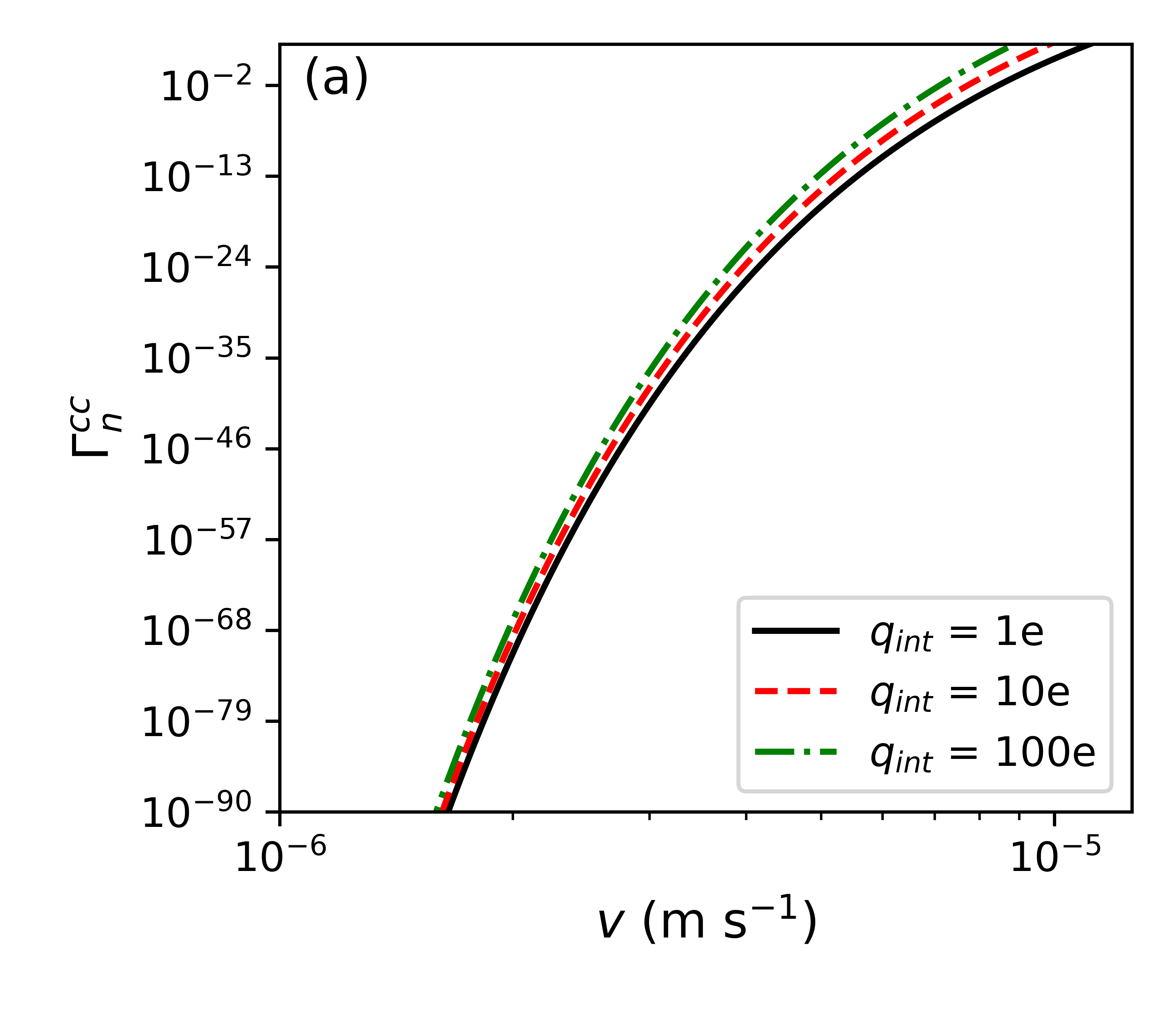
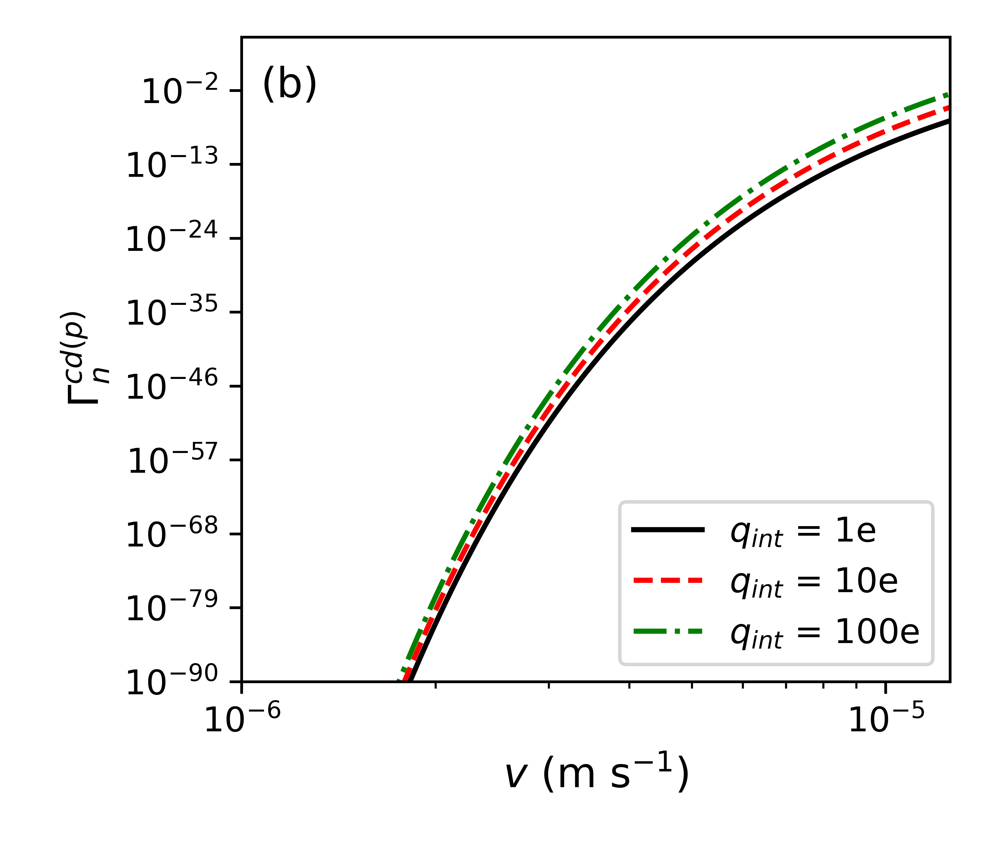
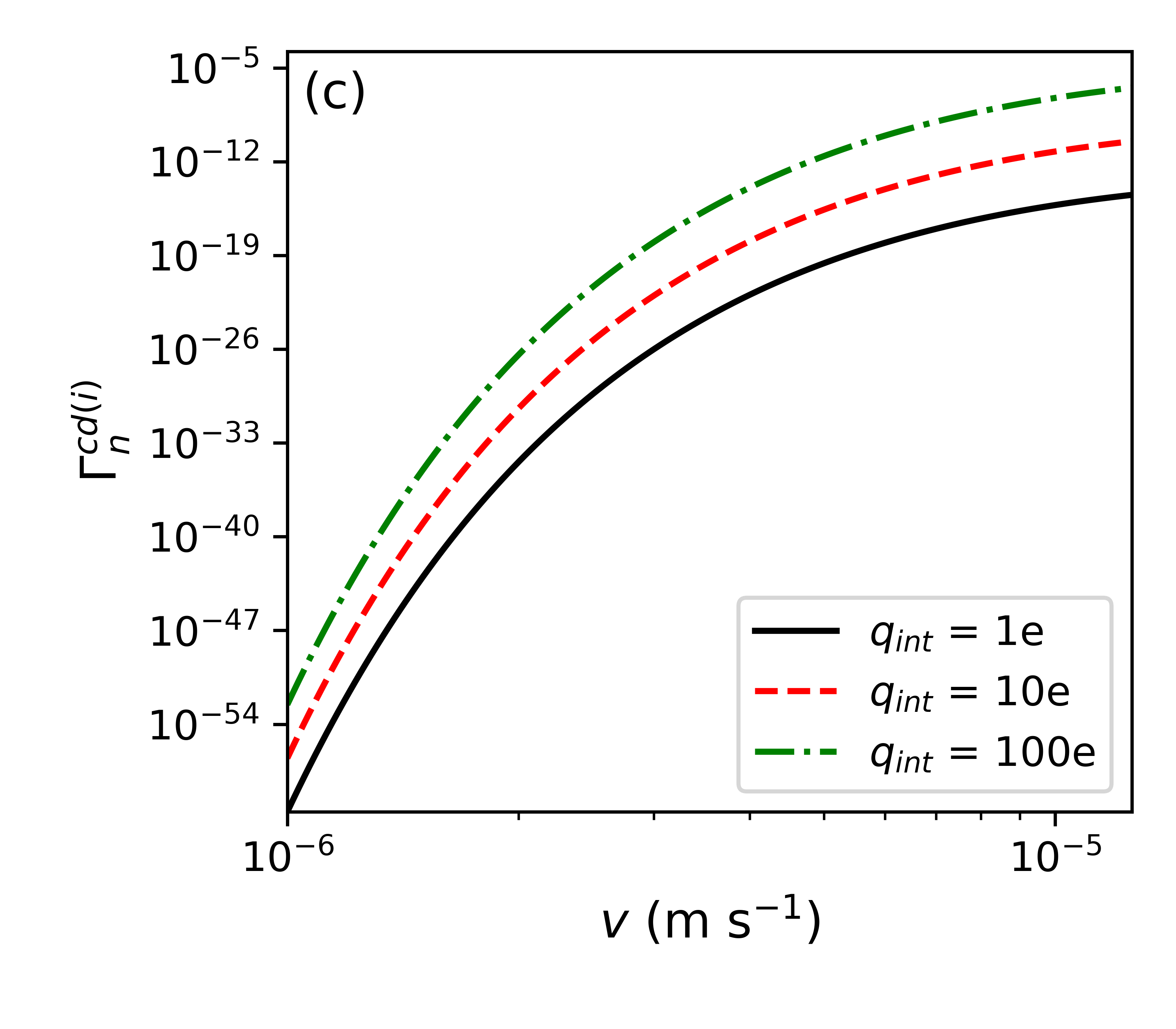
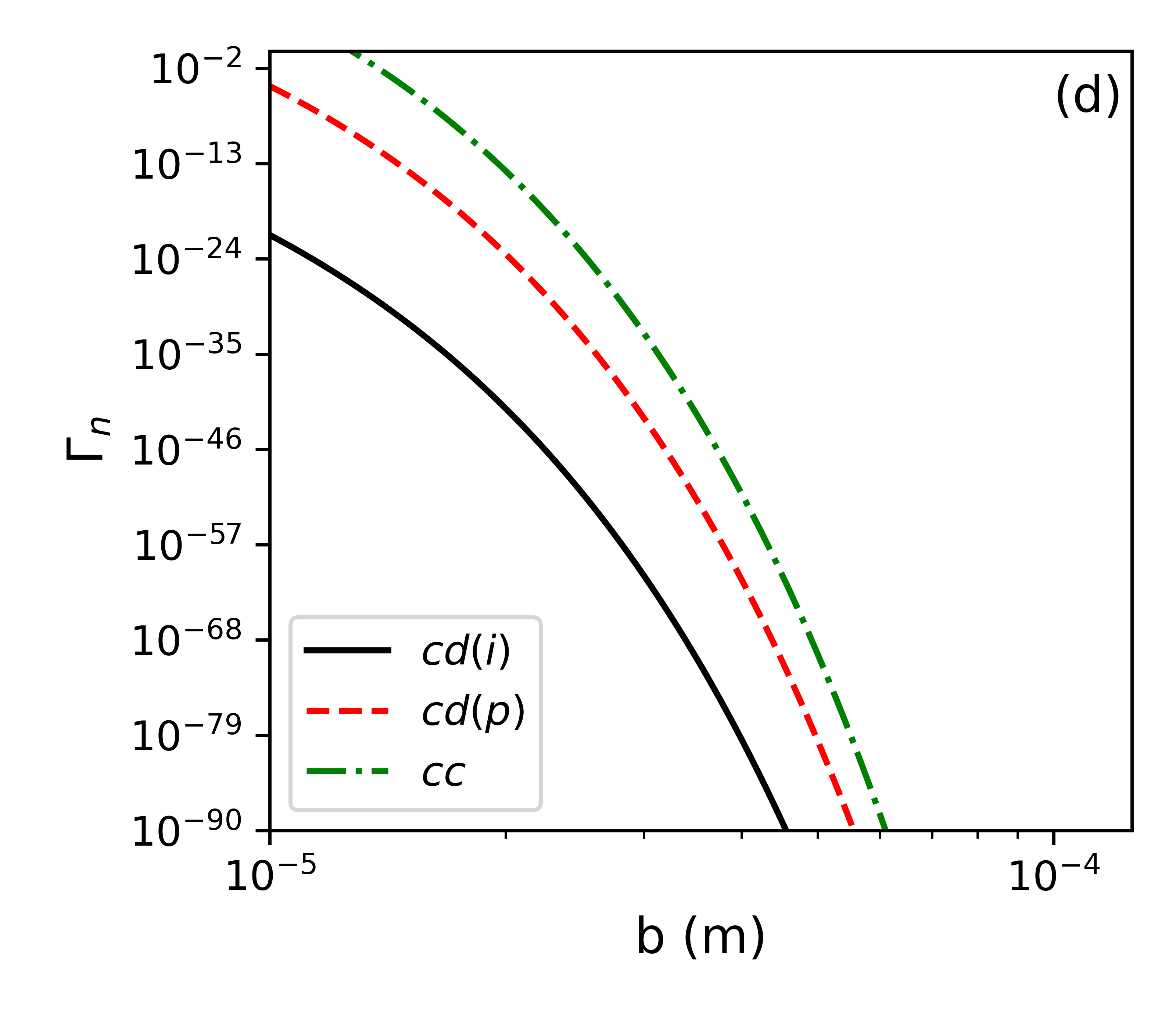
Figure 3: Dephasing as a function of the velocity of the external particle due to (a) the charge-charge interaction (cc), (b) the charge-permanent dipole interaction (cd(p)) and (c) the charge-induced dipole interaction (cd(i)), for a different number of interferometer charges. The expressions summarised in Tab. 1 are plotted, where the integral is solved numerically. With projection angles $\alpha=\beta=0$ and $T=b/v$. We have taken $\Delta x=20{\rm\mu m}$ in all the plots. In Fig.(a) $b=100\,$\mathrm{\SIUnitSymbolMicro m}$$ and the external charge is that of an electron, in Fig.(b) $b=100\,$\mathrm{\SIUnitSymbolMicro m}$$ and the external dipole moment $d_{\text{ext}}$ is that of a water molecule, in Fig.(c) $b=30\,$\mathrm{\SIUnitSymbolMicro m}$$ and the external particle’s polarizability is that of the dinitrogen. Fig.(d) shows the different dephasing for a charged interferometer as a function of the impact parameter, for $v=1\,$\mathrm{\SIUnitSymbolMicro m}\text{\,}{\mathrm{s}}^{-1}$$, $q_{\text{int}}=e$ and the interaction-specific parameters discussed above. This plot (d) shows that the interferometer could detect a $q_{\text{ext}}=e$ charged particle moving with a velocity $v=1\,$\mathrm{\SIUnitSymbolMicro m}\text{\,}{\mathrm{s}}^{-1}$$ in the vicinity of $10\,$\mathrm{\SIUnitSymbolMicro m}$$. The Coulomb interaction provides the largest dephasing compared to the charge dipole interactions. In all the plots we have ensured $T\sim b/v>\tau\sim 3\,$\mathrm{s}$$.

First, we discuss the dephasing for the charged micro-particle, discussed in Secs. IV. They are plotted in Fig. 3. Here, we specify the experimental parameters and summarise the dipole moment orientation and evolution assumptions. The dephasing that is plotted is given in Eqs. (26), (28) and (31) corresponding to dephasing in a charged interferometer. We will also discuss the possibility of the charged interferometer being an ideal quantum sensor to detect another electromagnetically charged particle moving in the vicinity.

The dephasing has been integrated in the frequency range from $\omega_{\text{min}}=2\pi/(t_{f}-t_{i})$ to $\omega=\infty$. The experiment time is set to be $\tau=t_{f}-t_{i}=4t_{a}+t_{e}$ (see figure 1). This frequency cut-off is chosen due to the frequency resolution of the discrete Fourier transform for the experimental setup. For the QGEM-specific example, we will take $\tau\sim 1$ s; for the CNOT gate, we will take $\tau\sim 1{\rm\mu s}$.

These parameters are chosen such that no acceleration jitter can be averaged beyond the experimental time. We have also optimised the projection angles, see Figs. 9-9, and the discussion in Appendix B. We have chosen the projection angles such that they maximise the dephasing. This will enable us to gauge the maximum acceleration noise the matter-wave interferometer can tolerate due to EM interactions. Also, it will help us do the total noise budget for the QGEM-type experiment Bose:2017nin and with the charged micro-particles Barker:2022mdz .

We have also plotted the dephasing given in Eqs. (36), (39) and (41) relating to the neutral micro-particle, which we will discuss below. While plotting this dephasing for the neutral micro-particle, we have made the following additional assumptions for the dipoles to obtain approximately the upper bounds on the dephasing. (1) In Eq. (28), the external dipole is assumed to align approximately with the vector $\hat{\bm{r}}(t)$ during the time of the experiment $\tau$. (2) In Eq. (36) the interferometer dipole is assumed to align with the $\hat{z}$-axis. (3) In Eq. (41) we have assumed both the above assumptions.

Other relevant parameters we have set are the maximum superposition size of $\Delta x=20\,\mu$m and $t_{a}=0.50$ s and $t_{e}=1.00$ s with total time $\tau=3$ s. Furthermore, we have taken the time scale over which the noise is averaged, $T\sim b/v>3$ s. We have also varied $T$ in Fig.4(a) for the neutral case for illustration.

VI.1 Dephasing of a charged micro-particle

As it is clear from the plots for the case of a charged micro-particle interferometer, the dephasing depends on the particle’s velocity $v$, and minimum impact parameter, which we have taken to be $b=10-100\,$\mathrm{\SIUnitSymbolMicro m}$$. The ambient particle is expected to have a small velocity $v\ll c$ for our analysis to be valid since we have excluded relativistic effects in the potentials. In Fig. 3(a), the dephasing grows as the velocity increases for a fixed $b$. The charge-charge case dominates the dephasing over other cases. This can be seen from Fig. 3(d). The Coulomb interaction is by far the most dominant source of dephasing for the charged interferometer; see Figs. 3(a-d). The charged interferometer can be treated as an excellent quantum sensor, sensing a charged ion moving with a velocity range of order $v\sim{\cal O}(10^{-1})\,{\rm m/s}$ in the vicinity of $b\sim 1$ m from the matter-wave interferometer (outside the range shown in the plot).

The dephasing due to charge-dipole interaction is shown in Fig. 3(b),(c). Fig (b) shows the charged micro-particle interacting with a molecule with a dipole interaction, where the external dipole is intrinsic to the external particle, for example, in a water molecule. The figure is plotted for a permanent dipole moment $\absolutevalue{\bm{d}_{\text{ext}}}\sim 6.17\times 10^{-30}\,$\mathrm{C}\text{\,}\mathrm{m}$$ of a water molecule lide2004crc , with $b=100\,$\mathrm{\SIUnitSymbolMicro m}$$. The dephasing is plotted as a function of the velocity of the external water molecule. For smaller velocities, the dephasing is small, but as the velocity increases, the dephasing increases, and it also increases with the charge of the micro-particle in the interferometer. We can see that the dephasing is small compared to the dephasing due to the Coulomb interaction.

Fig. 3(c) shows the dephasing due to the charged micro-particle and a dipole interaction where the external dipole is induced, for example, in the polarized air molecules. In this figure, we have taken the polarisability of di-nitrogen, ($1.710$Å${}^{3}=1.903\,$\mathrm{A}\mathrm{{}^{2}}\mathrm{s}^{4}\mathrm{/}\mathrm{k}\mathrm{g}$$), which is most frequently present air molecule, and impact parameter $b=30\,$\mathrm{\SIUnitSymbolMicro m}$$. Again, the dephasing is negligible.

We summarise our results in Fig. 3(d), which shows the dephasings due to charge-charge (cc), charge-permanent dipole (cd(p)) and charge-induced dipole (cd(i)) as a function of the impact parameter $b$ for $v=1\,$\mathrm{\SIUnitSymbolMicro m}\text{\,}{\mathrm{s}}^{-1}$$. The plot shows how the impact parameter $b$ influences dephasing in a fixed velocity scenario.

VI.2 Dephasing of a neutral micro-particle

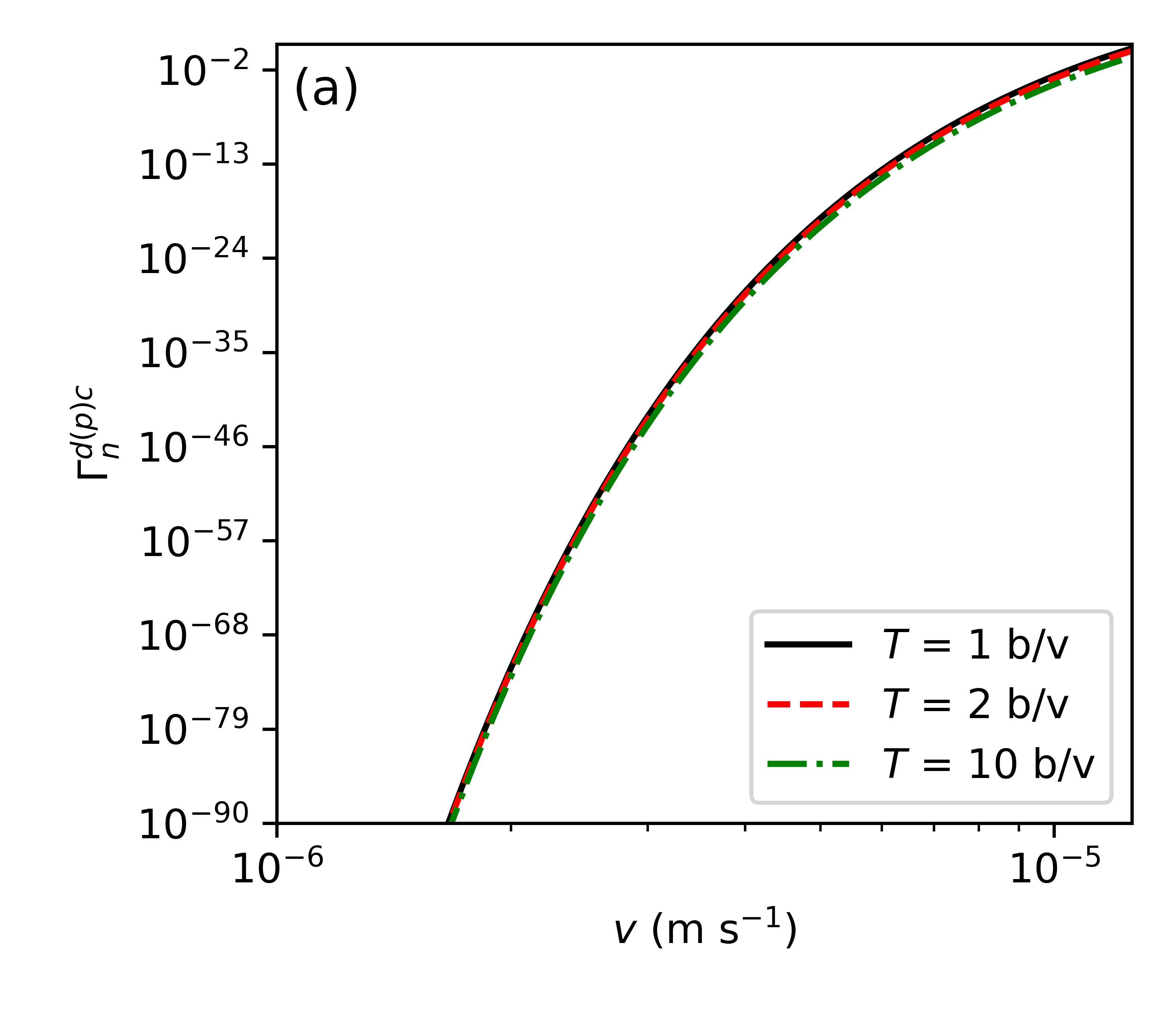
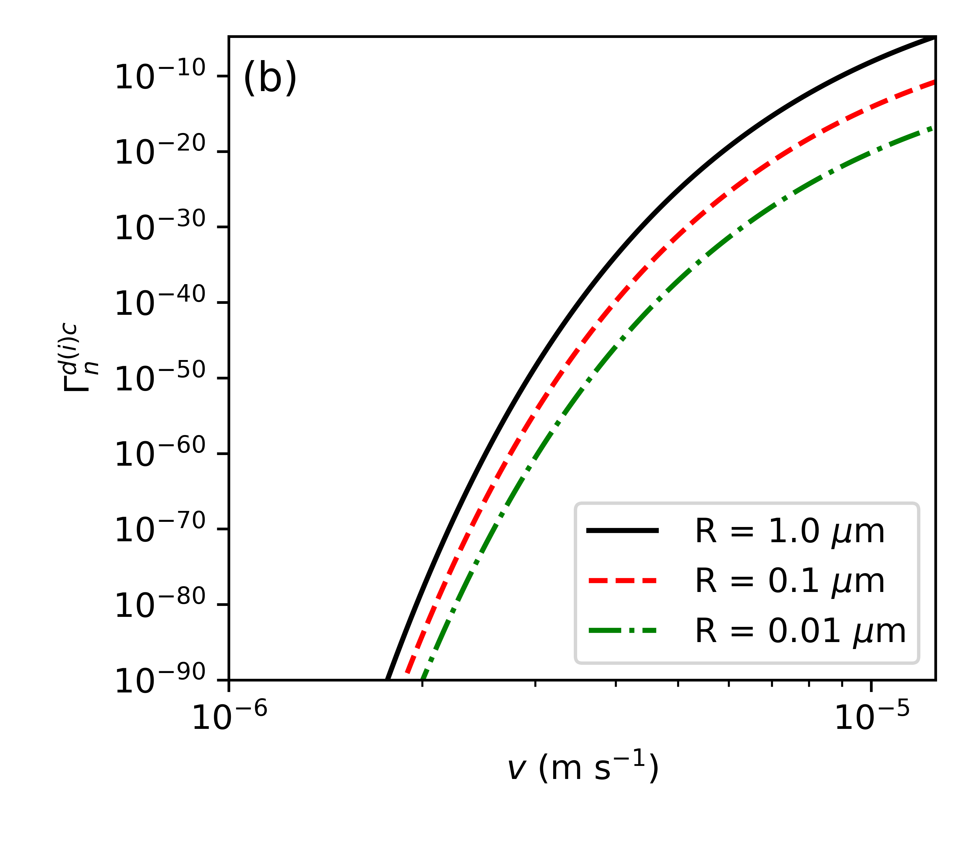
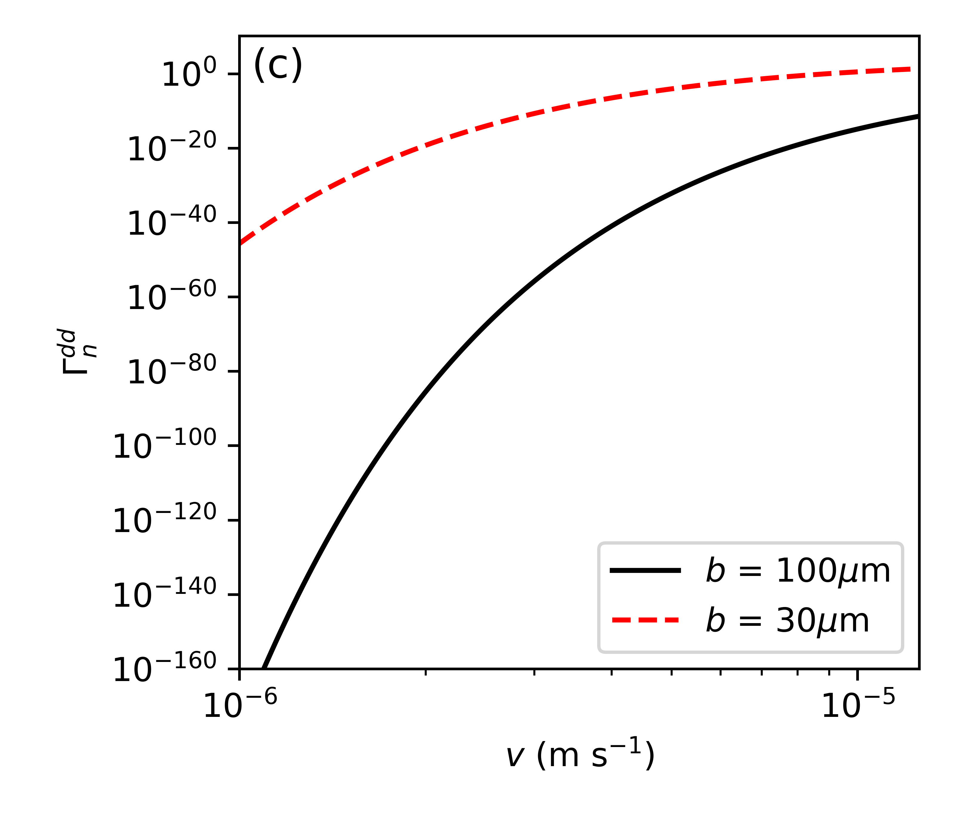
Figure 4: Dephasing due to (a) the permanent dipole-charge interaction (d(p)c), (b) the induced dipole-charge interaction (d(i)c) and (c) the dipole-dipole interaction (dd) as a function of the velocity of the external particle. The expressions summarised in Tab. 1 are plotted, where the integral is solved numerically. With projection angles $\alpha=\beta=\gamma=\theta_{0}=\pi/4$ for Fig. (a), $\alpha=\beta=0$ for Fig.(b), and $\alpha=\theta_{0}=\pi/4$, $\beta=0$ for Fig.(c), see Appendix B. We take $\Delta x=20{\rm\mu m}$ in all the cases. In Fig.(a) $b=100\,$\mathrm{\SIUnitSymbolMicro m}$$, $d_{\text{int}}=0.1e\,$\mathrm{\SIUnitSymbolMicro m}$$ and $q_{\text{ext}}=e$. Different lines for the noise time scale $T$ are shown. There is not much noticeable difference in the dephasing rate due to different values of $T=b/v$. In Fig.(b) $b=100\,$\mathrm{\SIUnitSymbolMicro m}$$, $d_{\text{int}}$ is induced by the external charge $q_{\text{ext}}=e$ (with $\epsilon_{r}=5.7$) and different lines for the interferometric particle’s radius are plotted. In Fig.(c) $d_{\text{int}}=0.1e\,$\mathrm{\SIUnitSymbolMicro m}$$ and the external particle is taken to be a water molecule, the dephasing is shown for different impact parameters. In Fig.(d), we summarise the dephasing from neutral micro-particles interactions as a function of the superposition width $\Delta x$, for $v=10\,$\mathrm{\SIUnitSymbolMicro m}\text{\,}{\mathrm{s}}^{-1}$$, $b=100\,$\mathrm{\SIUnitSymbolMicro m}$$, and the interaction-specific parameters discussed above for the charge and dipoles. The permanent dipole of a matterwave interferometer interacting with an external charge gives the largest dephasing here. We have ensured that $T=b/v>\tau\sim 3$ s.

In the case of a neutral interferometer, the results are shown in Fig. 4. Fig. 4(a) shows the dephasing due to the interaction of an intrinsic dipole of a micro-particle aligned at the $\hat{z}$-axis interacting with an external charge. We have taken the external particle to have the charge of an electron. Following the analysis in Appendix B, where we have chosen the angles to maximise the dephasing, the projection angles are considered $\alpha=\beta=\pi/2$. Furthermore, as an example, we have taken the impact parameter $b=100\,$\mathrm{\SIUnitSymbolMicro m}$$. In this plot, we have also shown different values of the $T\sim b/v$ parameter to show how the dephasing behaves with varying interaction times. As the velocity increases for a fixed impact parameter, the dephasing increases. Nevertheless, the dephasing remains very small for our analysis to be valid $T=b/v>\tau=3$ s.

Fig. 4(b) shows the dephasing due to the interaction between an external charge and the dipole it induces within the diamond microsphere. We have varied the mass of the micro diamond by changing the radius from $R\sim 1-0.01{\rm\mu m}$, and the dielectric constant of the diamond is taken to be $\epsilon_{r}=5.7$. The figure is very similar to (a), but the dephasing is significantly smaller (the plot is made for the impact parameter, $b=100\,$\mathrm{\SIUnitSymbolMicro m}$$). The dephasing would be further suppressed for smaller radii of the interferometer particle. In this case, the maximal projection angles were $\alpha=\beta=0$, which would maximise the dephasing; see Appendix B.

The dephasing due to the dipole-dipole interaction is given in fig. 4(c). Again, the interferometer is assumed to have a dipole aligned with the $\hat{z}$-axis of magnitude $\absolutevalue{\bm{d}_{\text{int}}}\sim 0.1e\,$\mathrm{\SIUnitSymbolMicro m}$\approx 1.6\times 10^{-26}\,$\mathrm{C}\text{\,}\mathrm{m}$$. The external dipole is assumed to be that of water, $\absolutevalue{\bm{d}_{\text{ext}}}\sim 6.17\times 10^{-30}\,$\mathrm{C}\text{\,}\mathrm{m}$$. Following the analysis in Appendix B the projection angles are taken to be $\alpha=\beta=\pi/2$, which gives the maximum dephasing, e.g. worst-case scenario, if $vt/b<1$. Different lines are shown for different impact parameters; one can see the dephasing is tiny.

It is worth pointing out that Ref. Fragolino:2023agd also studied the decoherence due to the dipole-dipole interactions in approximately the same parameter space. Specifically, the paper found the decoherence rate using the scattering model in the Born-Markov approximation. A direct comparison may not be valid, as the authors considered a quantum bath consisting of particles modelled as plane waves inside a box. In contrast, this paper considers a single external particle with classical trajectories. Still, comparing our analysis with the analysis from Fragolino:2023agd is interesting. As the underlying assumptions are different the predictions will in general differ, but a comparison nonetheless showed that when the impact factor $b$ from this analysis matches the size of the particle $R$ (and setting the number density corresponding to one environmental particle) the two predictions give the same order of magnitude prediction as expected (i.e., we match the length scale characterizing the distance between the system and environment to the same value in the two models).

Finally, Figs. 4(d) gives an overview of the dephasings described in Figs. (a)-(c) as a function of the superposition width, showing that a smaller superposition width reduces the dephasing. The most dominant source of dephasing is from the permanent dipole interacting with an external (electron) charge for $b=100\,$\mathrm{\SIUnitSymbolMicro m}$$ and $v=10\,$\mathrm{\SIUnitSymbolMicro m}\text{\,}{\mathrm{s}}^{-1}$$, which ensures $T\sim b/v>\tau$. The dephasing in all the cases is negligible.

VII Applications

We have discussed above the dephasing expressions for the charged and the neutral interferometers due to external charges and dipoles. We now discuss the applications for both the cases. The neutral interferometer is discussed in the context of the QGEM proposal for testing the quantum nature of gravity by witnessing the spin entanglement Bose:2017nin . We will also discuss the charged interferometer in the context of an ion-based quantum computer (where entanglement is due to the interaction of the photon between the two ions in adjacent ion traps) and study the dephasing due to the external charge and dipoles for a setup similar to the QGEM case.

VII.1 QGEM Protocol

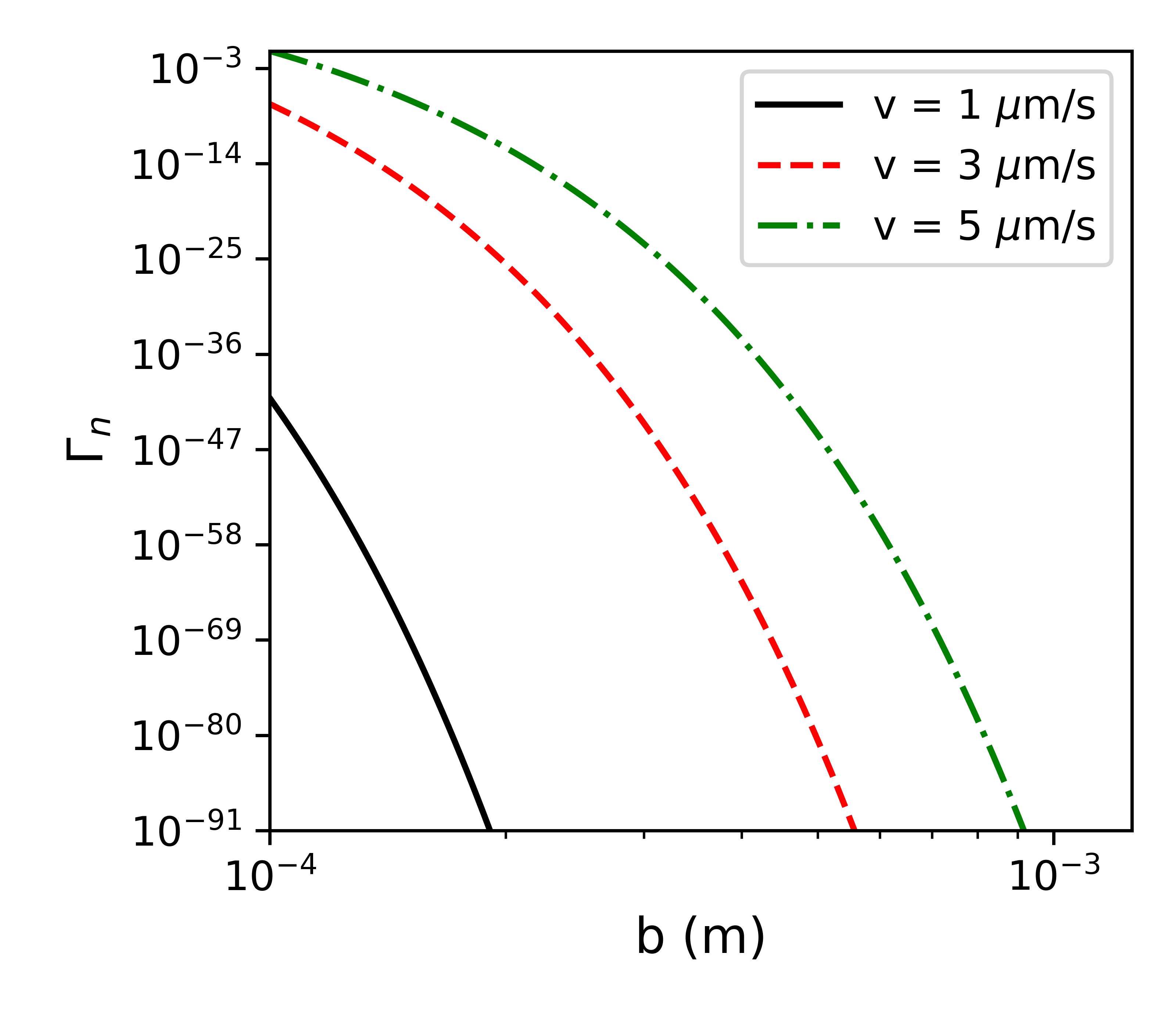
Figure 5: Dephasing for the QGEM microdiamond setup Schut:2023hsy . We consider the diamond to have a permanent dipole of the order of $0.1\,e\,$\mathrm{\SIUnitSymbolMicro m}$$, and mass $m=10^{-15}$ kg. We further assume that the maximum superposition size is $\Delta x=10\leavevmode\nobreak\ \mu\text{m}$ and that the total time is $\tau=1$ s. The dephasing is between the two interferometer arms, and can be assumed to be the same for both interferometers if they are separated by a distance $d\sim 50{\rm\mu m}\ll b$ (such that $b$ is the common impact factor of both interferometers). The noise is found from the sum of all the neutral interferometer interactions discussed in Figs. 4(a-d) now applied to the QGEM parameters. We take similar properties of the dipoles (induced and permanent) as that of Figs. 4(a-d). The dephasing is shown for different velocities of the external particle.

In the context of the QGEM protocol, details on which can be found here Bose:2017nin , we consider two neutral interferometers that are set up in a way such their spatial superposition directions are parallel Chevalier:2020uvv ; Tilly:2021qef ; Schut:2021svd ; Schut:2023eux ; Schut:2023hsy . For the purpose of illustration the paths of a single spatial interferometer is assumed to be as illustrated in figure 1. The initial spin state of the interferometers is given by:

$$\ket{\psi(0)}=\frac{1}{2}\left(\ket{\uparrow}_{1}+\ket{\downarrow}_{1}\right)\otimes\left(\ket{\uparrow}_{2}+\ket{\downarrow}_{2}\right)\,,$$ (42)

which is a separable state (see Sec. II for a short discussion on how the spin degrees of freedom are used to create spatial superposition states and then recombine the interferometric paths). A quantum gravitational interaction between the two massive interferometers will cause an entangling phase Bose:2017nin ; Marshman:2019sne ; Bose:2022uxe ; Danielson:2021egj ; Carney_2019 ; Carney:2021vvt ; Biswas:2022qto ; Christodoulou:2022vte ; Vinckers:2023grv ; Elahi:2023ozf ; Chakraborty:2023kel .

We will assume the hierarchy of lengths $b\gg d\gg\Delta x$ to simplify the analysis, such that $b$ can be taken as the impact factor for both interferometers, $d$ the distance between the center-of-mass of the two interferometers, and $\Delta x$ is the maximum superposition size of the individual interferometer. Taking into account the dephasing of the two interferometers, the final wavefunction at a time $t=\tau$ is described by:

$$\ket{\psi(\tau)}=\frac{e^{i\phi}e^{-i\delta\phi}}{2}\big{(} e^{i\delta\phi}\ket{\uparrow}_{1}\ket{\uparrow}_{2}+e^{i\Delta\phi}\ket{\uparrow}_{1}\ket{\downarrow}_{2}$$

$$+e^{i\Delta\phi}\ket{\downarrow}_{1}\ket{\uparrow}_{2}+e^{-i\delta\phi}\ket{\downarrow}_{1}\ket{\downarrow}_{2}\big{)}$$ (43)

with

$$\phi =\frac{\tau}{\hbar}\frac{Gm^{2}}{d}\,,\mbox{\quad\quad}\Delta\phi=\frac{\tau}{\hbar}\int_{0}^{\tau}\frac{Gm^{2}}{\sqrt{d^{2}+\Delta x^{2}(t)}}\,\differential{t}-\phi,$$ (44)

where $\delta\phi$ is the phase difference between the left and right arm of the interferometer due to interaction with the environmental particle, see Eq. (1).

The density matrix, $\rho$, is given by the final wavefunction, $\rho=\ket{\psi}\bra{\psi}$. Averaging over the different runs of the experiment, we find $\mathbb{E}[\rho]$. Treating $\delta\phi$ as a statistical quantity with $\mathbb{E}[\delta\phi]=0$ as discussed in Sec. II, and $\mathbb{E}[(\delta\phi)^{2}]=\Gamma_{n}$, see Eq. (9), the averaged density matrix is given by :

$\Gamma_{\text{n}}$ is given by the results found in the previous sections for the neutral micro-particle. To witness the entanglement due to the gravitational interaction, we use the positive partial transpose (PPT) witness, which, in the case of two qubits, provides a sufficient and necessary condition for entanglement based on the Peres-Horodecki criterion Horodecki:2009zz ; Tilly:2021qef ; Schut:2021svd . The PPT witness is defined as $\mathcal{W}=\ket{\lambda_{-}}\bra{\lambda_{-}}^{T_{2}}$, where $\ket{\lambda_{-}}$ is the eigenvector corresponding to the lowest eigenvalue, $\lambda_{-}$, of the partially transposed density matrix and the superscript $T_{2}$ denotes the partial transpose over system $2$. The witness for two interferometers aligned in a parallel way, corresponding to the wavefunction in Eq. (43), was found to be Schut:2023hsy :

$$\mathcal{W}=\frac{1}{4}(1\otimes 1-\sigma_{x}\otimes\sigma_{x}+\sigma_{z}\otimes\sigma_{y}+\sigma_{y}\otimes\sigma_{z})\,,$$ (46)

with $\sigma_{x},\sigma_{y},\sigma_{z}$ the Pauli spin matrices. The expectation value of the witness is given by Chevalier:2020uvv ; Tilly:2021qef ; Schut:2021svd :

$$\langle\mathcal{W}\rangle=\Tr(\mathcal{W}\rho)=\lambda_{-}.$$ (47)

For the wavefunction in Eq. (43) the expectation value is found to be:

$$\langle\mathcal{W}\rangle=\frac{1}{8}(1-e^{-2\Gamma_{n}})-\frac{1}{2}\sin(\absolutevalue{\Delta\phi})e^{-\Gamma_{\text{n}}/2}\,,$$ (48)

which reduces to the witness expectation value in Ref. Schut:2023hsy if $\Gamma_{n}=0$. The entanglement detection condition is $\langle\mathcal{W}\rangle<0$. If $\langle\mathcal{W}\rangle\geq 0$, there is no entanglement detection. Performing a short-time expansion of the witness, these inequalities can approximate the maximum allowed value of the dephasing rate:

$$2\Gamma_{\text{n}}-\frac{\absolutevalue{\Delta\phi}}{2}<0.$$ (49)

In paricular, if $\Gamma_{\text{n}}>\absolutevalue{\Delta\phi}/4$, then $\langle\mathcal{W}\rangle>0$ and there is no entanglement. Hence, the total dephasing due to the EM interaction must be $\Gamma_{n}<\absolutevalue{\Delta\phi}/4$ for the gravity-induced entanglement to be detectable.

We now accumulate all the sources of dephasing due to the EM interaction, such as arising from the Figs. 4(a-d), e.g. induced dipole-charge, permanent dipole-charge, and dipole-dipole interactions. In our case, we consider the diamond to have a permanent dipole of the order of $0.1\,e\,$\mathrm{\SIUnitSymbolMicro m}$$, and mass $m=10^{-15}$ kg. We further assume that the maximum superposition size is $\Delta x=10\leavevmode\nobreak\ \mu\text{m}$ and that the total time is $\tau=1$ s.

The cumulative effect of all the sources of dephasing for the QGEM experiment is shown in Fig. 5, where we have included the sum of all the electromagnetic dephasing sources affecting the interferometer consisting of a neutral particle. The transfer function of the interferometer is given Eq. (13), where the times $t_{e}$, $t_{a}$ are scaled-down compared to previous figures such that the total experimental time is $1\,$\mathrm{s}$$. For the external particle we have taken the same properties as in fig. 4(a-d). Naturally, as the velocity of the external particle increases and as the impact parameter decreases the dephasing increases, as expected. Nevertheless, the dephasing is so tiny that it will hardly be a problem for the QGEM experiment.

VII.2 CNOT Gate

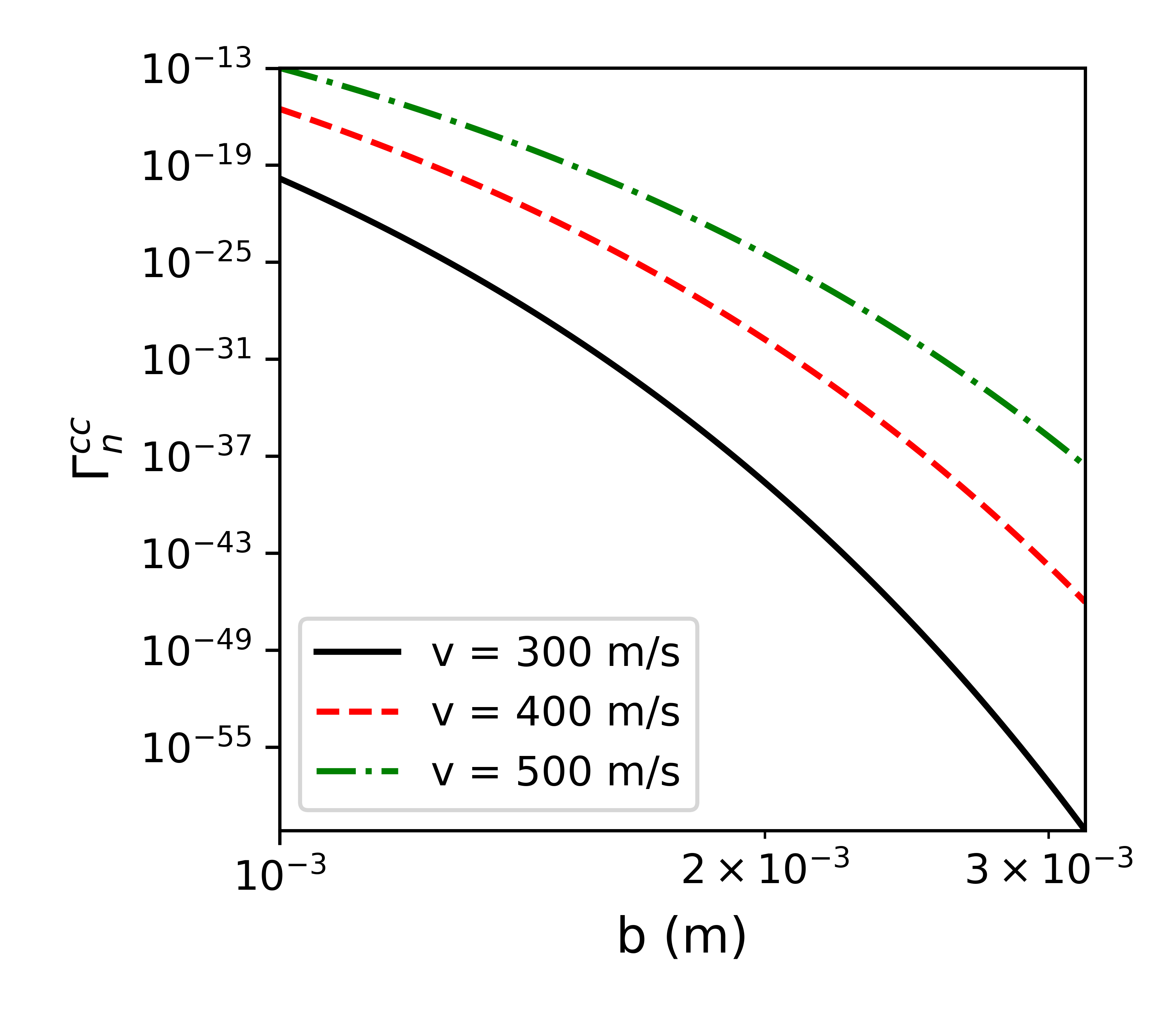
Figure 6: Charge-charge dephasing for ions of mass $m=10^{-27}\,$\mathrm{kg}$$ and charge $q_{\text{in}}=1e$ interacting with an external particle of charge $q_{\text{ext}}=10e$ as a function of the impact parameter $b$. The experimental time is $\tau=1\,$\mathrm{\SIUnitSymbolMicro s}$$ and the superposition size is assumed to be $\Delta x=0.18{\rm\mu m}$. The dephasing is shown for different velocities of the external particle.

In quantum computers, one often considers trapped charged particles Wineland:1992 ; Wineland:1995 . Here, we consider a CNOT gate consisting of two trapped ions separated by a distance $d$. Their initial wavefunction will be assumed to be prepared in a product state consisting of individual spatial superpositions. The entanglement between the two trapped ions will then build up due to the EM interaction mediated via photon, essentially the Coulomb interaction. If such a process generates a maximally entanglement state we have effectively created a CNOT gate. The final wavefunction of such an entangled system will be given by Eq. (43), with an entangled phase given by:

$$\phi =-\frac{\tau}{\hbar}\frac{\kappa_{e}q_{1}q_{2}}{d}\,,\Delta\phi=-\frac{\tau}{\hbar}\int_{0}^{\tau}\frac{\kappa_{e}q_{1}q_{2}}{\sqrt{d^{2}+\Delta x^{2}(t)}}\,\differential{t}-\phi\,,$$ (50)

where $\kappa_{e}=(4\pi\epsilon_{0})^{-1}$, and $q_{1}$ and $q_{2}$ are internal charges of the ions in their respective traps.

In Fig. 6, we show the dephasing $\Gamma^{cc}_{n}$ from the charge-charge Coulomb interaction. We have assumed that an external charge $q_{\text{ext}}=10e$ (which is not trapped) is flying by the ion traps with an impact parameter $b\gg d\gg\Delta x$ with a constant velocity $v$. We assume for simplicity that each trapped ion has mass $m\sim 10^{-27}\,$\mathrm{kg}$$, charge $q_{\text{in}}=q_{1}=q_{2}=1e$, and is trapped in a trap of frequency $\omega=10^{5}$ Hz. For concreteness, we can consider the size of the superposition size to be of the same order of magnitude as the zero point motion $\Delta x=\sqrt{\frac{\hbar}{2m\omega}}$, which for our parameters gives $\Delta x\sim 0.18{\rm\mu m}$. The entanglement builds up quite swiftly due to the Coulomb interaction, which is many orders of magnitude larger than the gravitational interaction strength. The total experimental time we require is $\tau=1\,$\mathrm{\SIUnitSymbolMicro s}$$ for the entanglement phase to be order unity assuming a trap separation $d=50{\rm\mu m}$. For illustration, we took a similar transfer function, which is responsible for creating the spatial superposition in Fig. 1. In our case, we have taken the external charge with different values of $b$ and $v$ to illustrate the scaling of the dephasing. Note that the dephasing increases if the impact parameter is small, and notably, a large constant velocity of a moving ion can create a significantly larger dephasing. As we see the dephasing is still small, e.g. $\Gamma^{(cc)}_{n}\sim 10^{-13}$ for $b\sim 10^{-3}$ m, $d\sim 50{\rm\mu m}$ and $v\sim 500{\rm m/s}$.

VIII Conclusion

In this paper we have adapted techniques established for investigating non-inertial and gravitational noise Toros:2020dbf ; Wu:2022rdv ; Saulson:1984 to compute the dephasing arising from the electromagnetic interactions. We considered two distinct scenarios, one where the micron size particle creating the superposition is charged and the other where the micron size particle is neutral. The main formulae are summarized in Table. 1.

The charged interferometer can interact via Coulomb interaction with an external charged particle. The external particle’s velocity is assumed to be constant, and the acceleration it will impart on both the arms of the interferometer will cause a jitter, which causes dephasing. The charged interferometer can also interact with a constantly moving dipole. The ambient particle can have a permanent dipole or an induced dipole. We considered both cases separately, see Figs. 3(a-d). The largest dephasing occurs due to the Coulomb interaction, which sets the exclusion zone for an externally charged particle.

In the neutral case, we have again four possibilities; a micro-particle is typically considered a diamond in our case, which has a dielectric property. The microdiamond can then have a permanent and an induced dipole; hence, it can interact with an external charge and an external dipolar particle, see Figs. 4(a-d). The external particle will impart a jitter in the trajectories due to the relative accelerations of the arms of the matterwave interferometer and, hence, will induce a dephasing.

If two neutral micro-particles, each prepared in spatial superpositions, and kept in an adjacent locations as in the case of the QGEM experiment Bose:2017nin , the relative acceleration noise is present in both test masses. This will cause a dephasing, as shown in Fig. 5, and hence leads to entanglement degradation. We found that it requires $\Gamma_{n}<\absolutevalue{\Delta\phi}/4$, with $\Gamma_{n}$ denoting the dephasing and $2\Delta\phi$ the entanglement phase, in order to witness entanglement in the QGEM setup (positive partial trace witness Chevalier:2020uvv ; Tilly:2021qef ; Schut:2021svd ). However, we have found that in the QGEM type experiment the dephasing from the external jitters due to the EM interactions is tiny for the parameter space considered in this paper.

The relative acceleration noise can also affect the ion trap-based spatial qubits, forming a CNOT gate. We observed that our methodology could be successfully employed to characterize the electromagnetic noise for such a setup. We found that for large velocities and small impact parameters, e.g., the distance between the externally charged particle and the two ion traps, the dephasing increases as shown in Fig. 6. The developed methodology could thus be used in estimating the decoherence budget.

However, our analysis has its limitations. We have only considered a single particle moving close to the matter-wave interferometer with a constant velocity. In our case, we can only model the noise if the velocity is non-relativistic and the trajectory of the external particles is approximately classical. We can bring two improvements; we can compute the dephasing for an ensemble of external particles, each responsible for dephasing the interferometer(s). The collective behaviour may shed light on how many ambient particles we can tolerate in the vicinity of the experiment. Moreover, we can further improve our techniques by considering the relativistic correction for the external particles.

Despite these challenges, we have provided a way of characterizing the noise in matter-wave interferometery due to external particles interacting via the EM interaction. Exploiting these techniques will be necessary for the success of fundamental problems such as witnessing of the quantum nature of gravity in a lab and could find applications for the design of future ion based quantum computers. Our analysis also provides an exciting sensing capability for a charged interferometer, which is sensitive to the Coulomb interaction, and could measure ${\cal O}(1)$ phase by choosing a sufficiently large superposition and charge of the interferometer. Such a sensor can be helpful to measure stray charges and characterize the environment of future experiments.

IX Acknowledgements

MS is supported by the Fundamentals of the Universe research program at the University of Groningen. MT acknowledges funding by the Leverhulme Trust (RPG-2020-197). S.B. would like to acknowledge EPSRC grants (EP/N031105/1, EP/S000267/1, and EP/X009467/1) and grant ST/W006227/1.

Appendix A Estimation of dephasing

This section shows the expressions for the Fourier transform of the acceleration, $a_{x}(\omega)$ and the corresponding PSD for the acceleration noise $S_{aa}(\omega)$, form which the dephasing due to the acceleration noise can be derived via

$$\Gamma_{\rm n}=\frac{1}{2\pi}\frac{m^{2}}{\hbar^{2}}\int_{\omega_{\rm min}}^{\infty}S_{aa}(\omega)F(\omega)\differential{\omega}\,.$$ (51)

with the transfer function $F(\omega)$ determined by the trajectory, see Eq. (13). Since,

$$a(\omega) =\int_{-\infty}^{\infty}a(t)e^{-i\omega t}\differential{t}$$ (52)

$$a(t) =\frac{1}{2\pi}\int_{-\infty}^{\infty}a(\omega)e^{i\omega t}\differential{\omega}$$ (53)

We rewrite the acceleration such that the Fourier transform can easily be performed:

$$a(b\omega/v)=\frac{b}{v}\int_{-\infty}^{\infty}a(vt/b)e^{-i(b\omega/v)(vt/b)}\differential{(vt/b)}\,.$$ (54)

The Fourier transform is of a function $f(vt/b)$ as defined below is given by:

$$f(vt/b) =\frac{(vt/b)^{2n}}{((vt/b)^{2}+c^{2})^{\nu+1/2}}$$ (55)

$$f(b\omega/v) =\frac{(-1)^{n}c^{\nu}\sqrt{\pi}}{2^{\nu}\Gamma(\nu+1/2)}\partialderivative[2n]{(b\omega/v)^{\nu}K_{\nu}(c\,b\omega/v)}{(b\omega/v)}$$

with $\Gamma(x)$ the Euler-Gamma-function  and $K_{\nu}$ the modified Bessel function of the second kind with order $\nu$. The above Fourier transform holds only if $\real(c)>0$ and $\real(\nu+1/2)>n$. The modified Bessel functions have the property that:

$$\partialderivative{K_{\nu}(x)}{x} =-\frac{1}{2}(K_{\nu-1}(x)+K_{\nu+1}(x))$$ (56)

$$K_{\nu-1}(x) =K_{\nu+1}(x)-\frac{2\nu}{x}K_{\nu}(x)$$

The modified Bessel functions with half-integers have the analytic formula:

$$K_{1/2}(u) =\sqrt{\frac{\pi}{2u}}\mathrm{e}^{-u}$$ (57)

$$K_{3/2}(u) =\sqrt{\frac{\pi}{2u}}\left(1+\frac{1}{u}\right)\mathrm{e}^{-u}$$

$$K_{5/2}(u) =\sqrt{\frac{\pi}{2u}}\left(1+\frac{3}{u}+\frac{3}{u^{2}}\right)\mathrm{e}^{-u}$$

The integer modified Bessel functions of the second kind do not have an analytical formula, but can be expressed in the integral form:

$$K_{0}(u) =\int_{0}^{\infty}\frac{\cos(tu)}{\sqrt{1+t^{2}}}\differential{t}$$ (58)

$$K_{1}(u) =\frac{1}{u}\int_{0}^{\infty}\frac{\cos(tu)}{(1+t^{2})^{3/2}}\differential{t}$$

$$K_{2}(u) =\frac{3}{u^{2}}\int_{0}^{\infty}\frac{\cos(tu)}{(1+t^{2})^{5/2}}\differential{t}$$

A.1 Charge-charge interaction

As presented in Eq. (25), the acceleration due to the charge-charge interaction in the $\hat{x}$-direction is:

$$a_{x}^{\text{cc}}(t)=\frac{q_{\text{int}}q_{\text{ext}}}{4\pi\epsilon_{0}mb^{2}}\frac{\cos(\alpha)+(vt/b)\cos(\beta)}{(1+(vt/b)^{2})^{3/2}}.$$ (59)

Transforming the acceleration $a_{x}^{\text{cc}}(t)$ into the frequency domain, we use Eq. (55) (with $c=1,\nu=1,n=0,1/2$) to obtain:

$$a_{x}^{\text{cc}}(\omega)=\frac{q_{\text{int}}q_{\text{ext}}\omega}{4\pi\epsilon_{0}mv^{2}}\bigg{[} \cos(\alpha)K_{1}\left(\frac{b\omega}{v}\right)$$ (60)

$$\,\,-i\cos(\beta)K_{0}\left(\frac{b\omega}{v}\right)\bigg{]}\,,$$

where $K_{\nu}(x)$ is a modified Bessel function, and we used its properties in Eq. (56). Note that after Fourier transform, the unit of $a_{x}(\omega)$ is $\rm m/(s^{2}\cdot Hz)$, which is because $a_{x}(t)=\int a_{x}(\omega)e^{i\omega t}d\omega$ has a unit $\rm m/s^{2}$ and $d\omega$ has a unit Hz.

Substituting Eq. 60 for the acceleration due to the Coulomb interaction into Eq. 6 for the PSD results in the desired PSD of the acceleration noise from the Coulomb interaction:

$$S_{aa}^{\text{cc}}(\omega)=\frac{q_{\text{int}}^{2}q_{\text{ext}}^{2}\omega^{2}}{16\pi^{2}Tm^{2}v^{4}\epsilon_{0}^{2}} \biggr{[}\cos^{2}(\alpha)K_{1}^{2}\left(\frac{b\omega}{v}\right)$$ (61)

$$+\cos^{2}(\beta)K_{0}^{2}\left(\frac{b\omega}{v}\right)\biggr{]}.$$

Note that the unit of $S_{aa}(\omega)=|a_{x}(\omega)|^{2}/T$ is $\rm m^{2}/(s^{4}\cdot Hz)$. Using Eq. (51) gives the dephasing in Eq. (26).

A.2 Charge-dipole interaction

A.2.1 Permanent dipole

As presented in Eq. (27), the acceleration due to the charge-permanent dipole interaction in the $\hat{x}$-direction is:

$$a_{x}^{\text{cd(p)}}(t)=\frac{q\absolutevalue{\mathbf{d}_{\text{ext}}}}{2\pi mb^{3}\epsilon_{0}}\frac{\cos(\alpha)+(vt/b)\cos(\beta)}{(1+(vt/b)^{2})^{2}}\,.$$ (62)

Transforming the acceleration $a_{x}^{\text{cd(p)}}(t)$ into the frequency domain, we use Eq. (55) (with $c=1,\nu=3/2,n=0,1/2$) to obtain:

$$a_{x}^{\text{cd(p)}}({\omega})=\frac{q|\mathbf{d}_{\text{ext}}|\omega^{3/2}}{4\pi\epsilon_{0}mv^{3/2}b^{3/2}}\sqrt{\frac{\pi}{2}} \frac{b}{v}\Bigg{[}\cos(\alpha)K_{3/2}\left(\frac{b\omega}{v}\right)$$ (63)

$$-i\cos(\beta)K_{1/2}\left(\frac{b\omega}{v}\right)\Bigg{]}\,.$$

where $K_{\nu}(x)$ is a modified Bessel function, and we used its properties in Eq. (56).

Now substituting this expression into definition of the PSD of the acceleration noise results in:

$$S_{aa}^{\text{cd(p)}}(\omega)=\frac{q^{2}|\mathbf{d}_{\text{ext}}|^{2}\omega^{3}}{32\pi Tm^{2}v^{5}b\epsilon_{0}^{2}} \Biggr{[}\cos^{2}(\alpha)K_{3/2}^{2}\left(\frac{b\omega}{v}\right)$$ (64)

$$+\cos^{2}(\beta)K_{1/2}^{2}\left(\frac{b\omega}{v}\right)\Biggr{]}.$$

The resulting dephasing is given in Eq. (28).

A.2.2 Induced dipole

As presented in Eq. (30), the acceleration due to the charge-permanent dipole interaction in the $\hat{x}$-direction is:

$$a_{x}^{\text{cd(i)}}(t)=\frac{q^{2}_{\text{int}}\alpha_{\text{pol}}}{8\pi^{2}mb^{5}\epsilon_{0}^{2}}\frac{\cos(\alpha)+(vt/b)\cos(\beta)}{(1+(vt/b)^{2})^{3}}.$$

Performing a Fourier transform given in Eq. (55) (with $c=1,\nu=5/2,n=0,1/2$) to find the acceleration in the frequency domain gives:

$$a_{x}^{\text{cd(i)}}(\omega)=\frac{q^{2}\alpha_{\text{pol}}\omega^{5/2}}{64\pi^{2}mb^{3/2}v^{7/2}\epsilon_{0}^{2}} \sqrt{\frac{\pi}{2}}\Biggr{[}\cos(\alpha)K_{5/2}\left(\frac{b\omega}{v}\right)$$ (65)

$$-i\cos(\beta)K_{3/2}\left(\frac{b\omega}{v}\right)\Biggr{]}.$$

Substituting this expression into definition of the PSD of the acceleration noise results in a slightly modified expression compared to the permanent dipole case:

$$S_{aa}^{\text{cd(i)}}(\omega)=\frac{q^{4}\alpha^{2}_{\text{pol}}\omega^{5}}{8192\pi^{3}m^{2}v^{7}b^{3}\epsilon_{0}^{4}T}\Biggr{[} \cos^{2}(\alpha)K^{2}_{5/2}\left(b\omega/v\right)$$ (66)

$$+\cos^{2}(\beta)K^{2}_{3/2}(b\omega/v)\Biggr{]}.$$

The resulting dephasing is given in Eq. (31).

A.3 Dipole-charge interaction

A.3.1 Permanent dipole

As presented in Eq. (35) the acceleration in the $\hat{x}$-direction due to the permanent dipole interacting with an external charge is:

$$a_{x}^{\text{d(p)c}}(t)=\frac{q_{\text{ext}}|\mathbf{d}_{\text{int}}|}{2\pi mb^{3}\epsilon_{0}} \frac{\cos(\alpha)+(vt/b)\cos(\beta)}{(1+(vt/b)^{2})^{5/2}}$$ (67)

$$\bigg{[}\cos(\theta_{0})+(vt/b)\cos(\gamma)\bigg{]},$$

The second line comes from the resolution of the dot product as:

$$\bm{d}_{\text{int}}\cdot\hat{\bm{r}}(t) =\absolutevalue{\bm{d}_{\text{int}}}\frac{b_{z}+v_{z}t}{r(t)}\,,$$ (68)

$$=\absolutevalue{\bm{d}_{\text{int}}}\frac{\cos(\theta_{0})+(vt/b)\cos(\gamma)}{\sqrt{1+(vt/b)^{2}}}\,,$$ (69)

where we have assumed that the direction of the dipole vector of the interferometer is constant, i.e. $\bm{d}_{\text{int}}$ is not time-dependent, and that it points in the $\hat{z}$-direction. For example, because the microdiamond sphere is magnetically trapped Marshman:2023nkh and its rotational degrees of freedom are cooled to near its ground state Deli__2020 , achieving good control of the system.

In the second line above, Eq. (69) we have written the dot product in terms of the angle $\theta_{0}$, which is the angle between the $\hat{z}$-axis and the vector $b$, and the angle $\gamma$ which gives the $\hat{z}$-component of the velocity:

$$b_{z}=b\cos(\theta_{0})\,,\mbox{\quad\quad}v_{z}=v\cos(\gamma)\,.$$ (70)

The Fourier transform of the acceleration $a_{x}^{\text{d(p)c}}(t)$ is found from Eq. (55) (with $c=1,\nu=2,n=0,1/2,1$) and gives:

Where we used Eqs. (55) to find the Fourier transform and Eqs. (56) to simplify the expression.

Now substituting this expression into the Eq. (5) of the PSD of the acceleration noise results in:

$$S_{aa}^{\text{d(p)c}}(\omega) =\frac{q_{\text{ext}}^{2}|\mathbf{d}_{\text{int}}|^{2}\omega^{4}}{36\pi^{2}\epsilon_{0}^{2}m^{2}v^{6}T}\Bigg{[}\cos^{2}(\alpha)\bigg{(}K_{2}^{2}\left(\frac{b\omega}{v}\right)$$

$$\cos^{2}(\theta_{0})+K_{1}^{2}\left(\frac{b\omega}{v}\right)\cos^{2}(\gamma)\bigg{)}$$

$$+\cos^{2}(\beta)\bigg{(}K_{1}^{2}\left(\frac{\omega}{bv}\right)\cos^{2}(\theta_{0})$$

$$+\bigg{[}\frac{b\omega}{v}K_{1}\left(\frac{b\omega}{v}\right)-K_{0}\left(\frac{b\omega}{v}\right)\bigg{]}^{2}\cos^{2}(\gamma)\bigg{)}\Bigg{]}\,.$$

The resulting dephasing from Eq. (51) and (13) is given by:

$$\Gamma_{\operatorname{n}}^{\text{d(p)c}} =\frac{4q_{\text{ext}}^{2}|\mathbf{d}_{\text{int}}|^{2}(\Delta x)^{2}}{9\pi^{3}\epsilon_{0}^{2}\hbar^{2}v^{6}t_{a}^{4}}\int^{\infty}_{\omega_{\text{min}}}\frac{1}{\omega^{2}}\sin^{4}\left(\frac{t_{a}\omega}{2}\right)$$ (72)

$$\Bigg{[}\cos^{2}(\alpha)\bigg{(}K_{2}^{2}\left(\frac{b\omega}{v}\right)\cos^{2}(\theta_{0})$$

$$\mbox{\quad\quad}+K_{1}^{2}\left(\frac{b\omega}{v}\right)\cos^{2}(\gamma)\bigg{)}$$

$$+\cos^{2}(\beta)\bigg{(}K_{1}^{2}\left(\frac{b\omega}{v}\right)\cos^{2}(\theta_{0})+\bigg{[}\frac{b\omega}{v}K_{1}\left(\frac{b\omega}{v}\right)$$

$$-K_{0}\left(\frac{b\omega}{v}\right)\bigg{]}^{2}\cos^{2}(\gamma)\bigg{)}\Bigg{]}\sin^{2}\left(\frac{\omega}{2}(2t_{a}+t_{e})\right)\differential{\omega}$$

Which has been presented in Eq. (36) in a simplified form.

A.3.2 Induced dipole

Eq. (38) gave the acceleration in the $\hat{x}$-direction for the interaction between an external charge and the dipole it induces in the interferometer:

$$a_{x}^{\text{d(i)c}}(t) =\frac{\epsilon_{r}-1}{\epsilon_{r}+2}\frac{q_{\text{ext}}^{2}R^{3}}{2\pi\epsilon_{0}mb^{5}}\frac{\cos(\alpha)+(vt/b)\cos(\beta)}{(1+(vt/b)^{2})^{3}}$$ (73)

Performing a Fourier transform to find the acceleration in the frequency domain gives (from Eq. (55) with $c=1,\nu=5/2,n=0,1/2$):

$$a_{x}^{\text{d(i)c}}(\omega)= \frac{\epsilon_{r}-1}{\epsilon_{r}+2}\frac{q_{\text{ext}}^{2}R^{3}\omega^{5/2}}{16\pi mb^{5/2}v^{5/2}\epsilon_{0}}\frac{b}{v}\sqrt{\frac{\pi}{2}}$$

$$\Biggr{[}\cos(\alpha)K_{5/2}\left(\frac{b\omega}{v}\right)-i\cos(\beta)K_{3/2}\left(\frac{b\omega}{v}\right)\Biggr{]}.$$ (74)

Substituting this expression into the PSD of the acceleration noise results in a slightly modified expression compared to the permanent dipole case:

$$S_{aa}^{\text{d(i)c}}= \left(\frac{\epsilon_{r}-1}{\epsilon_{r}+2}\right)^{2}\frac{q_{\text{ext}}^{4}R^{6}\omega^{5}}{512\pi\epsilon_{0}^{2}m^{2}v^{7}b^{3}T}$$ (75)

$$\Biggr{[}\cos^{2}(\alpha)K^{2}_{5/2}\left(\frac{b\omega}{v}\right)+\cos^{2}(\beta)K^{2}_{3/2}\left(\frac{b\omega}{v}\right)\Biggr{]}\,,$$

from which Eq. (39) is derived.

A.4 Dipole-dipole interaction

The acceleration due to dipole-dipole interactions is given by griffiths2013introduction :

$$\bm{a}_{\text{dd}}=\frac{3\,\hat{\bm{r}}}{4\pi\epsilon_{0}m}\left[\frac{\bm{d}_{\text{ext}}\cdot\bm{d}_{\text{int}}}{r^{4}(t)}-3\frac{(\bm{d}_{\text{ext}}\cdot\hat{\bm{r}})(\bm{d}_{\text{int}}\cdot\hat{\bm{r}})}{r^{4}(t)}\right]$$ (76)

In order to resolve the dot products, we recall from previous sections the assumption we have made, that

1. The external particle has low velocity, meaning that $\bm{d}_{\text{ext}}\cdot\hat{\bm{r}}$ is approximately constant in time. Furthermore, in the worst-case scenario $\bm{d}_{\text{ext}}\cdot\hat{\bm{r}}=\absolutevalue{\bm{d}_{\text{ext}}}$.

2. The dipole of the interferometer particle is aligned with the $\hat{z}$-axis. Such that $\bm{d}_{\text{int}}\cdot\hat{\bm{r}}$ is as in Eq. (69). Assuming that the external particle has small velocity, $\bm{d}_{\text{int}}\cdot\hat{\bm{r}}\approx\absolutevalue{\bm{d}_{\text{int}}}\cos(\theta_{0})$.

From the orientation of the dipoles in these assumptions, it follows that:

1. The angle between the interferometer and external dipoles is $\theta_{0}$, such that $\bm{d}_{\text{int}}\cdot\bm{d}_{\text{ext}}=\absolutevalue{\bm{d}_{\text{int}}}\absolutevalue{\bm{d}_{\text{ext}}}\cos(\theta_{0})$.

In this scenario, the acceleration in the $\hat{x}$-direction becomes:

$$\bm{a}^{\text{dd}}_{x}(t) =-\frac{6}{4\pi\epsilon_{0}m}\frac{\absolutevalue{\bm{d}_{\text{ext}}}\absolutevalue{\bm{d}_{\text{int}}}\cos(\theta_{0})}{r^{4}(t)}\frac{\bm{r}_{x}}{r}$$

$$=-\frac{6\absolutevalue{\bm{d}_{\text{ext}}}\absolutevalue{\bm{d}_{\text{int}}}\cos(\theta_{0})}{4\pi\epsilon_{0}mb^{4}}\frac{\cos(\alpha)+(vt/b)\cos(\beta)}{(1+(vt/b)^{2})^{5/2}}$$

as presented in Eq. (40). Using the Fourier transform in Eq. (55) and the properties given in Eq. (56) gives:

$$a_{x}^{\text{dd}}(\omega)= \frac{2\absolutevalue{\bm{d}_{\text{ext}}}\absolutevalue{\bm{d}_{\text{int}}}\cos(\theta_{0})}{4\pi\epsilon_{0}m}\frac{\omega^{2}}{bv^{3}}$$

$$\Bigg{[}\cos(\alpha)K_{2}\left(\frac{b\omega}{v}\right)-i\cos(\beta)K_{1}\left(\frac{b\omega}{v}\right)\Bigg{]}$$ (77)

which gives the PSD of the acceleration noise:

$$S_{aa}^{\text{dd}}(\omega)= \frac{\absolutevalue{\bm{d}_{\text{ext}}}^{2}\absolutevalue{\bm{d}_{\text{int}}}^{2}\cos^{2}(\theta_{0})}{4\pi^{2}\epsilon_{0}^{2}m^{2}T}\frac{\omega^{4}}{b^{2}v^{6}}$$

$$\Bigg{[}\cos^{2}(\alpha)K_{2}^{2}\left(\frac{b\omega}{v}\right)+\cos^{2}(\beta)K_{1}^{2}\left(\frac{b\omega}{v}\right)\Bigg{]}$$ (78)

Which, together with the transfer function, gives the dephasing due to the dipole-dipole interaction, as given in Eq. (41).

Appendix B Projection angles analysis

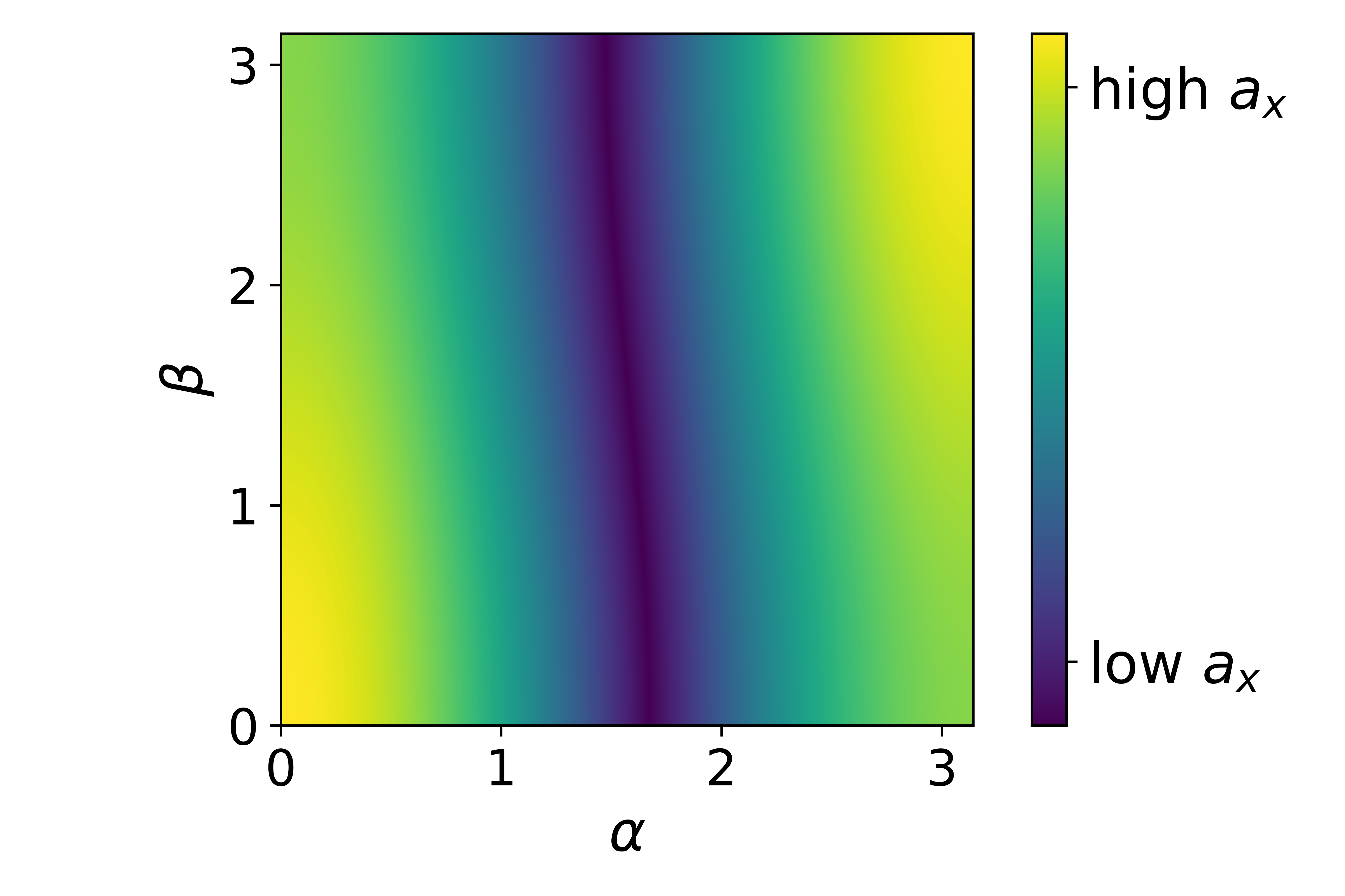
Figure 7: For $vt/b=0.1$ the absolute value of the acceleration (Eq. (79) with $a=3$) as a function of the projection angles $\alpha,\beta\in[0,\pi]$.

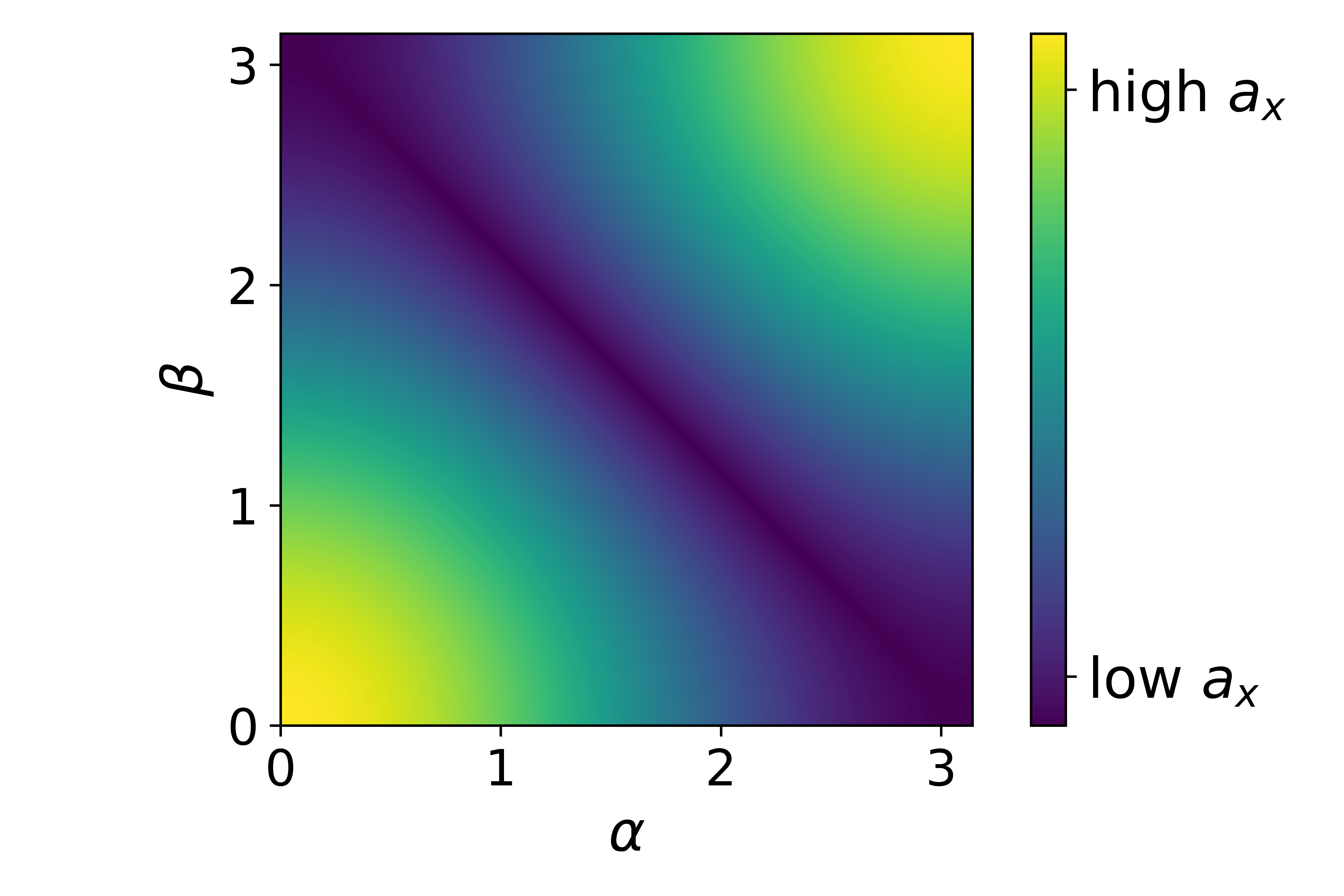
Figure 8: For $vt/b=1$ the absolute value of the acceleration (Eq. (79) with $a=3$) as a function of the projection angles $\alpha,\beta\in[0,\pi]$.

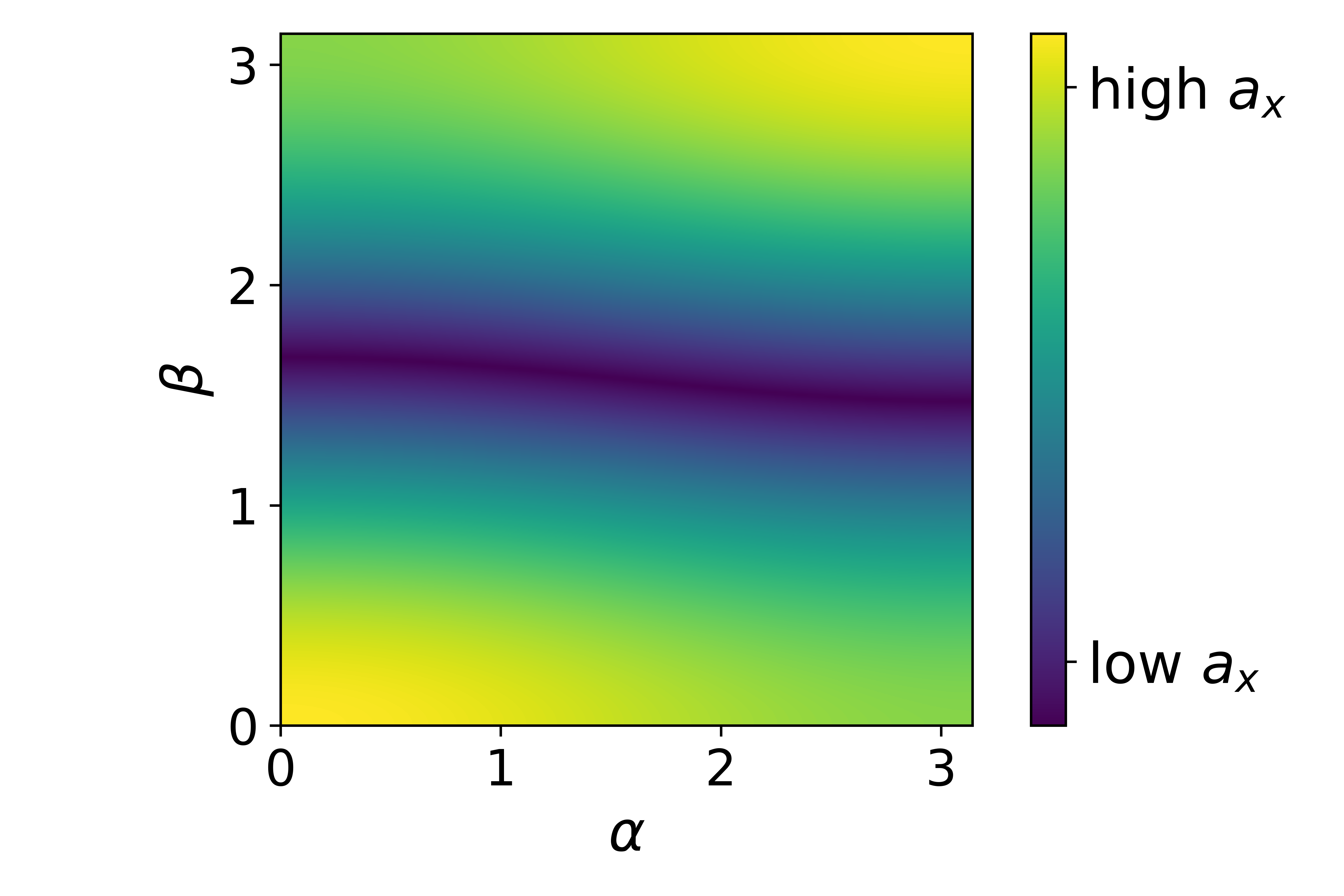
Figure 9: For $vt/b=10$ the absolute value of the acceleration (Eq. (79) with $a=3$) as a function of the projection angles $\alpha,\beta\in[0,\pi]$.

To maximize the dephasing, we take the initial conditions as given by the projections angels $\alpha$ and $\beta$ (respectively, b and $v$ in the $\hat{x}$-direction) and in the case of an interferometer dipole $\theta_{0}$ and $\gamma$ (respectively, b and $v$ in the $\hat{z}$-direction), such that the absolute value of the acceleration in the $\hat{x}$-direction is maximal.

By maximising the acceleration, the noise is also maximised since the transfer function $S_{aa}(t)\propto a(t)^{2}$ and $\Gamma_{\text{n}}\propto S_{aa}(\omega)F(\omega)$, where the transfer function $F(\omega)$ is independent of the projection angles. Physically it is clear that a larger acceleration causes a larger dephasing.

B.1 Charged interferometer

For a charged interferometer, the relevant angles that determine the movement of the external particle are $\alpha$ and $\beta$; see Eq. (15). To find an upper bound on the dephasing, these angles are maximised. The figs. 9-9 show the acceleration

$$a(t)=\absolutevalue{C\frac{\cos(\alpha)+(vt/b)\cos(\beta)}{(1+(vt/b)^{2})^{a}}}$$ (79)

as a function of the angles $\alpha$ and $\beta$. The magnitude of the acceleration is not given since it depends on the constant $C$, which is determined by the type of interaction (charged-charged, charged-permanent dipole or charged-induced dipole). The value $a$ is also specified by the type of interaction, $a=3/2,2,3$, see Eqs. (25), (27), (30).

The figures show that for $vt>b$ by at least one order of magnitude the acceleration is maximised for $\beta=0,\pi$ and $\alpha$ arbitrary. If $vt<b$ by at least one order of magnitude then the plot rotates ninety degrees and the maximum value of the acceleration is given by $\alpha=0,\pi$ and $\beta$ arbitrary. For $vt\sim b$ the maximisation is given by $\alpha=\beta=0$ or $\alpha=\beta=\pi$. The Figs. 9-9 are approximately constant for $a=3/2,2,3$.

Therefore a simple way to choose the angles such that the absolute acceleration from the interaction is maximised is to choose $\alpha=\beta=0$ (or $\pi$) .

B.2 Neutral interferometer

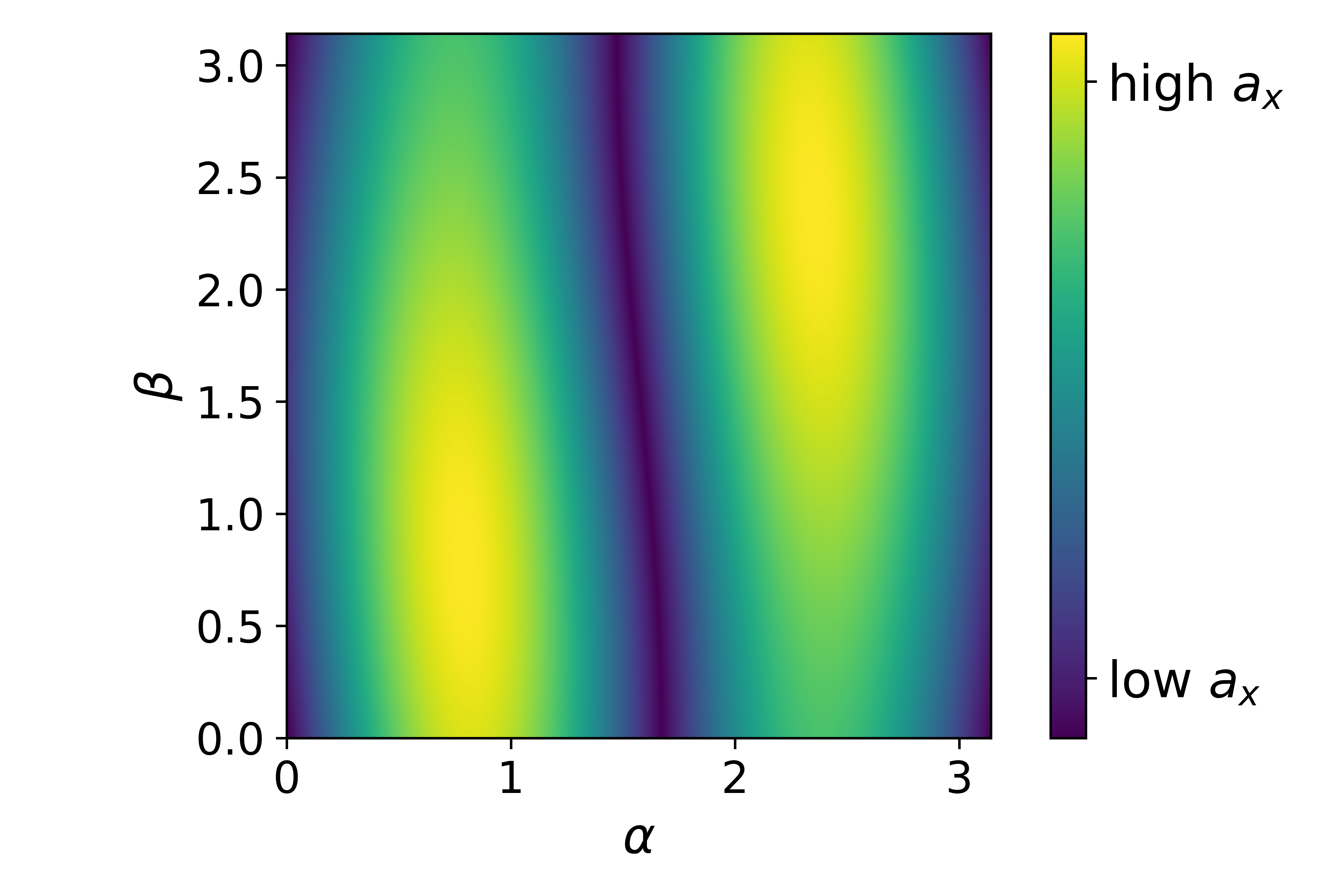
Figure 10: For $vt/b=0.1$ the absolute value of the acceleration (Eq. (80)) as a function of the projection angles $\alpha,\beta\in[0,\pi]$.

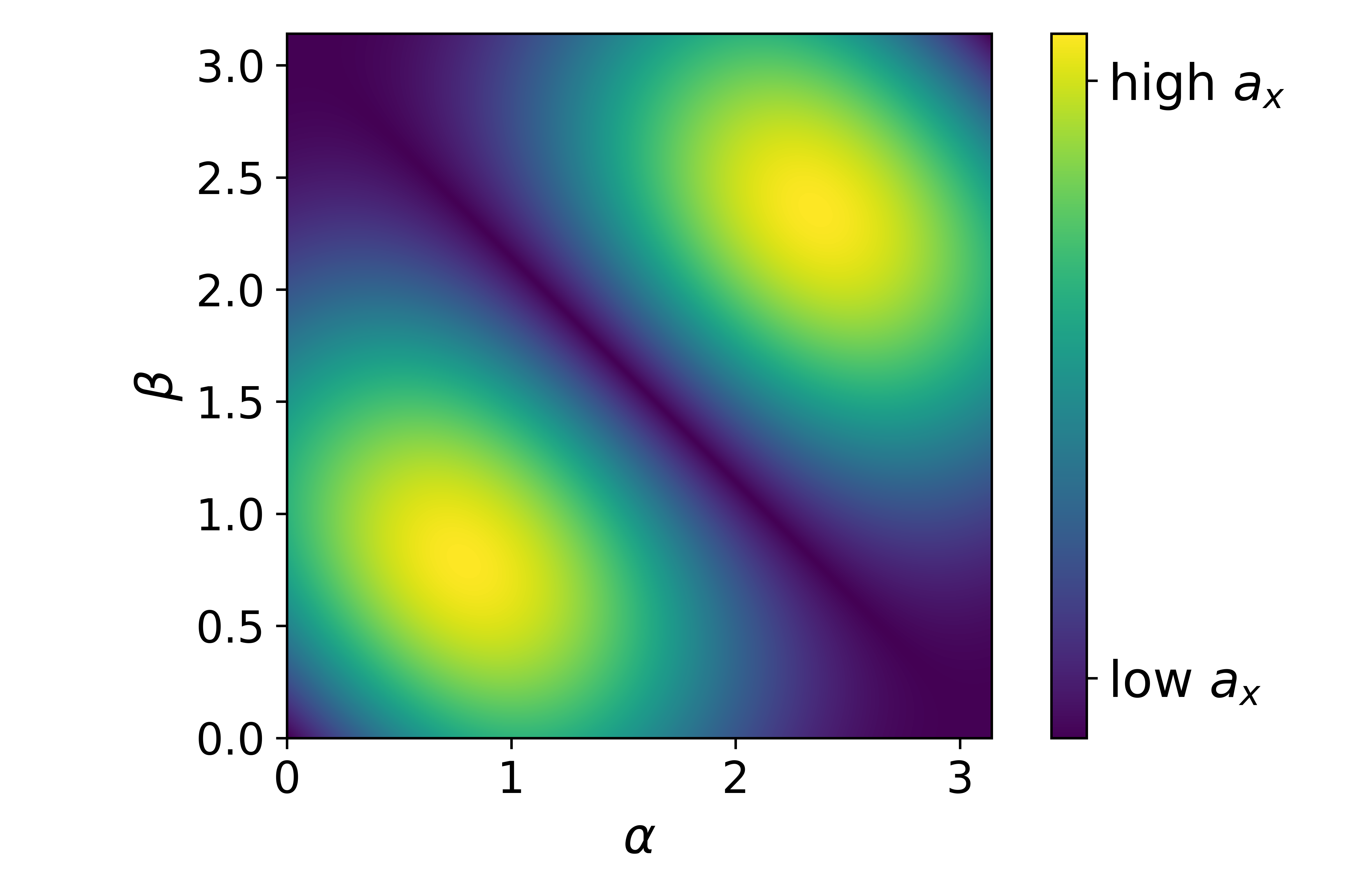
Figure 11: For $vt/b=1$ the absolute value of the acceleration (Eq. (80)) as a function of the projection angles $\alpha,\beta\in[0,\pi]$.

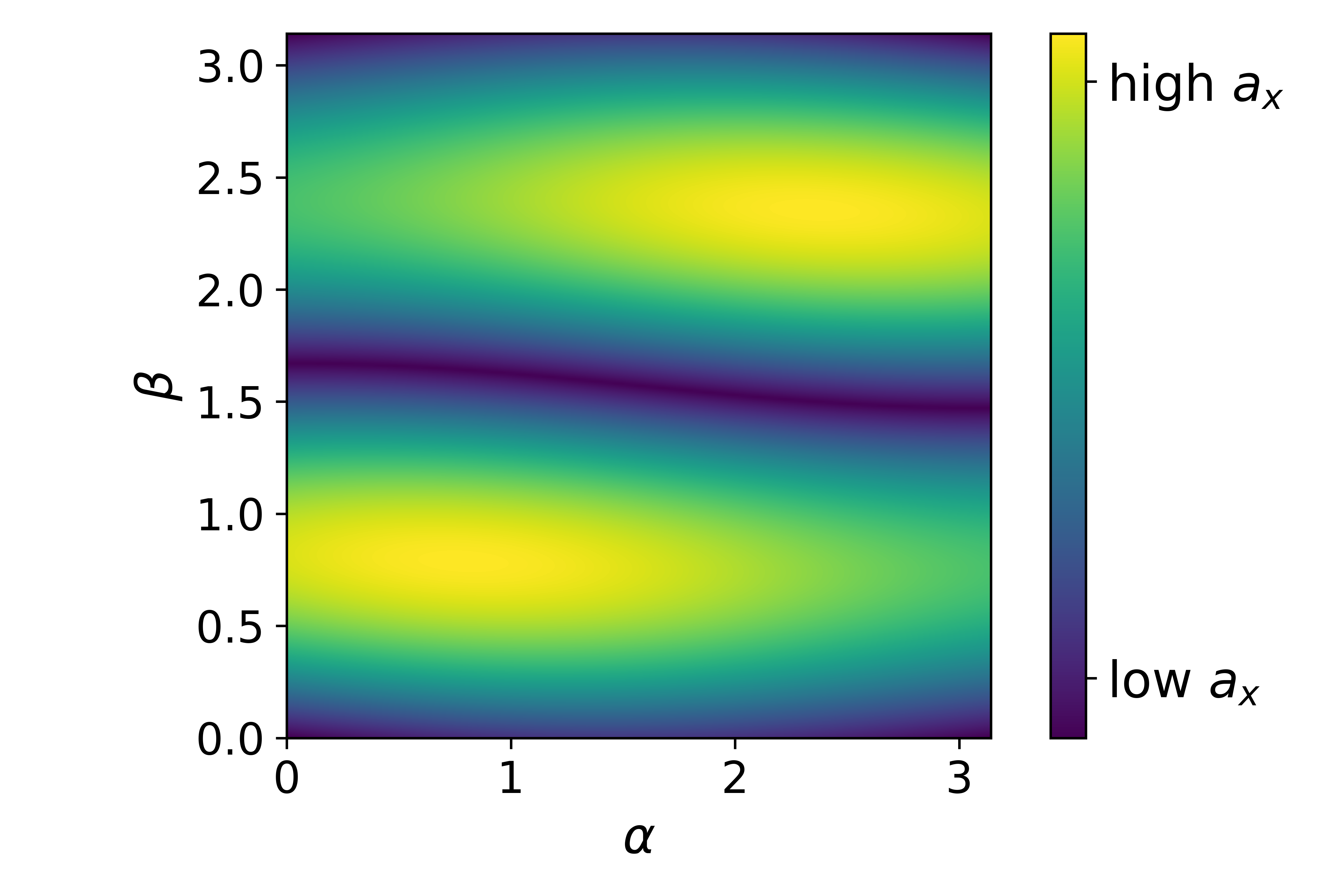
Figure 12: For $vt/b=10$ the absolute value of the acceleration (Eq. (80)) as a function of the projection angles $\alpha,\beta\in[0,\pi]$.

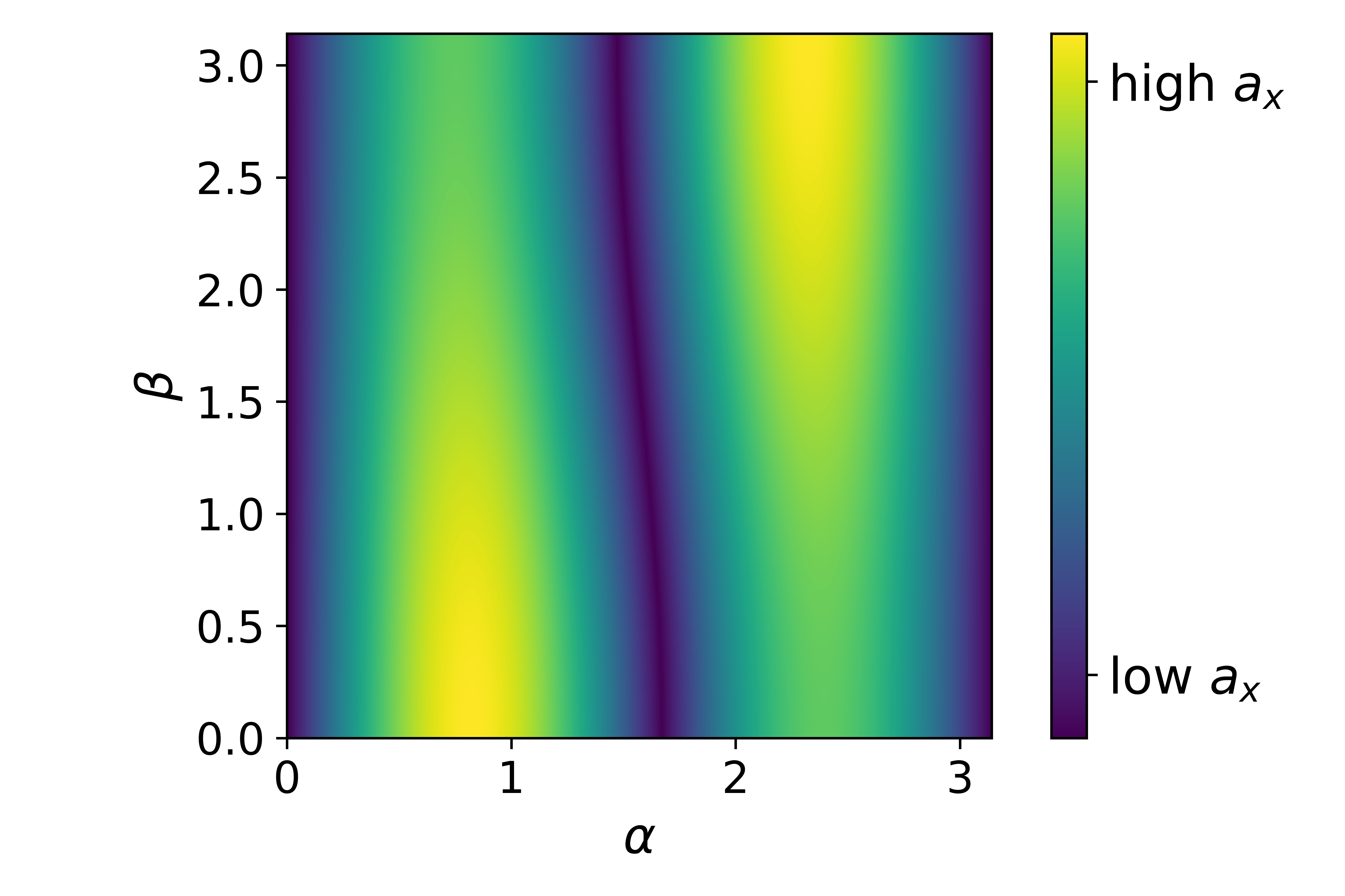
Figure 13: For $vt/b=0.1$ the absolute value of the acceleration for the dipole case (Eq. (80) without the $\cos(\gamma)$-term) as a function of the projection angles $\alpha,\beta\in[0,\pi]$.

For a neutral interferometer there are the additional angles $\gamma$ and $\theta_{0}$ that give the projection in the $\hat{z}$-axis, see Eq. (70) . They are relevant because the interferometer dipole has been chosen to align with the $\hat{z}$-axis.

Generically, we write the acceleration in the $\hat{x}$-direction from the dipole-charge and dipole-dipole interactions as:

$$a(t)=\absolutevalue{C\frac{\cos(\alpha)+(vt/b)\cos(\beta)}{(1+(vt/b)^{2})^{5/2}}\left(\cos(\theta_{0})+(vt/b)\cos(\gamma)\right)}$$ (80)

with $C$ a constant defined by the interaction. The angles $\alpha$ and $\theta_{0}$ are related in the sense that if $\alpha=0$, it means that $b=x_{0}$, and therefore $\theta_{0}=\pi/2$ such that $b_{z}=0$. Similarly the angles $\beta$ and $\gamma$ are related such that if $\beta=0$, $v=v_{x}$ and thus $\gamma=\pi/2$, such that $v_{z}=0$. Therefore, we define the dependency as

$$\cos(\theta_{0})=\sqrt{1-\cos^{2}(\alpha)},\,\,\,\cos(\gamma)=\sqrt{1-\cos^{2}(\beta)}.$$ (81)

This follows from Pythagoras theorem $v^{2}=v_{x}^{2}+v_{y}^{2}+v_{z}^{2}$, where for maximisation of the acceleration, we have set $v_{y}=0$.

The resulting plots that show the acceleration of Eq. (80) as a function of $\alpha$, $\beta$ for arbitrary $C$ are shown in Figs. 13-13. The figures are somewhat similar to Figs. 9-9, but one can see the extra dependence on the projection angles. From the figures, we can conclude that in order to maximise the acceleration in a generic way one can take the projection angles $\alpha=\beta=\pi/4,3\pi/4$, which means that $\theta_{0}=\gamma=\pi/4,3\pi/4$.

In the case of a dipole-dipole interaction, the assumption that the particle has low velocity such that $\bm{r}(t)\cdot\bm{d}$ is approximately constant in time removes the dependence on $\gamma$. The resulting plot looks very similar to Fig. 13 and shows that the acceleration is maximal for $\alpha=\pi/4$, $\beta=0$ and for $\alpha=3\pi/4$ and $\beta=\pi$, see Fig. 13.

References

- (1) L. De Broglie, “Waves and quanta,” Nature, vol. 112, no. 2815, pp. 540–540, 1923.
- (2) G. P. Thomson and A. Reid, “Diffraction of cathode rays by a thin film,” Nature, vol. 119, no. 3007, pp. 890–890, 1927.
- (3) C. Davisson and L. H. Germer, “Diffraction of electrons by a crystal of nickel,” Physical review, vol. 30, no. 6, p. 705, 1927.
- (4) C. J. Davisson and L. H. Germer, “Reflection and refraction of electrons by a crystal of nickel,” Proceedings of the National Academy of Sciences, vol. 14, no. 8, pp. 619–627, 1928.
- (5) E. Schrodinger, “Die gegenwartige Situation in der Quantenmechanik,” Naturwiss., vol. 23, pp. 807–812, 1935.
- (6) R. Colella, A. W. Overhauser, and S. A. Werner, “Observation of gravitationally induced quantum interference,” Physical Review Letters, vol. 34, no. 23, p. 1472, 1975.
- (7) V. V. Nesvizhevsky, H. G. Börner, A. K. Petukhov, H. Abele, S. Baeßler, F. J. Rueß, T. Stöferle, A. Westphal, A. M. Gagarski, G. A. Petrov, et al., “Quantum states of neutrons in the earth’s gravitational field,” Nature, vol. 415, no. 6869, pp. 297–299, 2002.
- (8) J. B. Fixler, G. Foster, J. McGuirk, and M. Kasevich, “Atom interferometer measurement of the newtonian constant of gravity,” Science, vol. 315, no. 5808, pp. 74–77, 2007.
- (9) P. Asenbaum, C. Overstreet, T. Kovachy, D. D. Brown, J. M. Hogan, and M. A. Kasevich, “Phase shift in an atom interferometer due to spacetime curvature across its wave function,” Physical review letters, vol. 118, no. 18, p. 183602, 2017.
- (10) C. Overstreet, P. Asenbaum, J. Curti, M. Kim, and M. A. Kasevich, “Observation of a gravitational aharonov-bohm effect,” Science, vol. 375, no. 6577, pp. 226–229, 2022.
- (11) R. J. Marshman, A. Mazumdar, G. W. Morley, P. F. Barker, S. Hoekstra, and S. Bose, “Mesoscopic Interference for Metric and Curvature (MIMAC) Gravitational Wave Detection,” New J. Phys., vol. 22, no. 8, p. 083012, 2020.
- (12) E. Kilian, M. Toroš, F. F. Deppisch, R. Saakyan, and S. Bose, “Requirements on quantum superpositions of macro-objects for sensing neutrinos,” Phys. Rev. Res., vol. 5, no. 2, p. 023012, 2023.
- (13) P. F. Barker, S. Bose, R. J. Marshman, and A. Mazumdar, “Entanglement based tomography to probe new macroscopic forces,” Phys. Rev. D, vol. 106, no. 4, p. L041901, 2022.
- (14) A. Einstein, B. Podolsky, and N. Rosen, “Can quantum-mechanical description of physical reality be considered complete?,” Physical review, vol. 47, no. 10, p. 777, 1935.
- (15) J. S. Bell, “On the einstein podolsky rosen paradox,” Physics Physique Fizika, vol. 1, no. 3, p. 195, 1964.
- (16) R. Horodecki, P. Horodecki, M. Horodecki, and K. Horodecki, “Quantum entanglement,” Rev. Mod. Phys., vol. 81, pp. 865–942, 2009.
- (17) S. Bose, A. Mazumdar, G. W. Morley, H. Ulbricht, M. Toroš, M. Paternostro, A. Geraci, P. Barker, M. S. Kim, and G. Milburn, “Spin Entanglement Witness for Quantum Gravity,” Phys. Rev. Lett., vol. 119, no. 24, p. 240401, 2017.
- (18) https://www.youtube.com/watch?v=0Fv-0k13s_k, 2016. Accessed 1/11/22.
- (19) C. Marletto and V. Vedral, “Gravitationally-induced entanglement between two massive particles is sufficient evidence of quantum effects in gravity,” Phys. Rev. Lett., vol. 119, no. 24, p. 240402, 2017.
- (20) C. H. Bennett, D. P. DiVincenzo, J. A. Smolin, and W. K. Wootters, “Mixed state entanglement and quantum error correction,” Phys. Rev. A, vol. 54, pp. 3824–3851, 1996.
- (21) R. J. Marshman, A. Mazumdar, and S. Bose, “Locality and entanglement in table-top testing of the quantum nature of linearized gravity,” Phys. Rev. A, vol. 101, no. 5, p. 052110, 2020.
- (22) S. Bose, A. Mazumdar, M. Schut, and M. Toroš, “Mechanism for the quantum natured gravitons to entangle masses,” Phys. Rev. D, vol. 105, no. 10, p. 106028, 2022.
- (23) A. Soerensen and K. Moelmer, “Quantum computation with ions in thermal motion,” Phys. Rev. Lett., vol. 82, pp. 1971–1974, 1999.
- (24) D. Biswas, S. Bose, A. Mazumdar, and M. Toroš, “Gravitational optomechanics: Photon-matter entanglement via graviton exchange,” Phys. Rev. D, vol. 108, no. 6, p. 064023, 2023.
- (25) S. Bose, A. Mazumdar, M. Schut, and M. Toroš, “Entanglement Witness for the Weak Equivalence Principle,” 2022.
- (26) S. Chakraborty, A. Mazumdar, and R. Pradhan, “Distinguishing Jordan and Einstein frames in gravity through entanglement,” 10 2023.
- (27) S. G. Elahi and A. Mazumdar, “Probing massless and massive gravitons via entanglement in a warped extra dimension,” 3 2023.
- (28) U. K. B. Vinckers, A. de la Cruz-Dombriz, and A. Mazumdar, “Quantum entanglement of masses with non-local gravitational interaction,” 3 2023.
- (29) F. Hanif, D. Das, J. Halliwell, D. Home, A. Mazumdar, H. Ulbricht, and S. Bose, “Testing whether gravity acts as a quantum entity when measured,” 7 2023.
- (30) T. W. van de Kamp, R. J. Marshman, S. Bose, and A. Mazumdar, “Quantum Gravity Witness via Entanglement of Masses: Casimir Screening,” Phys. Rev. A, vol. 102, no. 6, p. 062807, 2020.
- (31) M. Scala, M. S. Kim, G. W. Morley, P. F. Barker, and S. Bose, “Matter-wave interferometry of a levitated thermal nano-oscillator induced and probed by a spin,” Phys. Rev. Lett., vol. 111, p. 180403, Oct 2013.
- (32) C. Wan, M. Scala, G. W. Morley, A. A. Rahman, H. Ulbricht, J. Bateman, P. F. Barker, S. Bose, and M. S. Kim, “Free nano-object ramsey interferometry for large quantum superpositions,” Phys. Rev. Lett., vol. 117, p. 143003, Sep 2016.
- (33) Y. Margalit et al., “Realization of a complete Stern-Gerlach interferometer: Towards a test of quantum gravity,” Science Advances, vol. 7, 11 2020.
- (34) R. J. Marshman, A. Mazumdar, R. Folman, and S. Bose, “Constructing nano-object quantum superpositions with a Stern-Gerlach interferometer,” Phys. Rev. Res., vol. 4, no. 2, p. 023087, 2022.
- (35) S. Machluf, Y. Japha, and R. Folman, “Coherent stern–gerlach momentum splitting on an atom chip,” Nature Communications, vol. 4, p. 2424, 09 2013.
- (36) O. Amit, Y. Margalit, O. Dobkowski, Z. Zhou, Y. Japha, M. Zimmermann, M. A. Efremov, F. A. Narducci, E. M. Rasel, W. P. Schleich, and R. Folman, “ stern-gerlach matter-wave interferometer,” Phys. Rev. Lett., vol. 123, p. 083601, Aug 2019.
- (37) Y. Margalit, Z. Zhou, O. Dobkowski, Y. Japha, D. Rohrlich, S. Moukouri, and R. Folman, “Realization of a complete stern-gerlach interferometer,” arXiv preprint arXiv:1801.02708, 2018.
- (38) R. Zhou, R. J. Marshman, S. Bose, and A. Mazumdar, “Catapulting towards massive and large spatial quantum superposition,” Phys. Rev. Res., vol. 4, no. 4, p. 043157, 2022.
- (39) R. Zhou, R. J. Marshman, S. Bose, and A. Mazumdar, “Mass-independent scheme for enhancing spatial quantum superpositions,” Phys. Rev. A, vol. 107, no. 3, p. 032212, 2023.
- (40) R. Zhou, R. J. Marshman, S. Bose, and A. Mazumdar, “Gravito-diamagnetic forces for mass independent large spatial quantum superpositions,” 11 2022.
- (41) R. J. Marshman, S. Bose, A. Geraci, and A. Mazumdar, “Entanglement of Magnetically Levitated Massive Schrödinger Cat States by Induced Dipole Interaction,” 4 2023.
- (42) M. Schut, J. Tilly, R. J. Marshman, S. Bose, and A. Mazumdar, “Improving resilience of quantum-gravity-induced entanglement of masses to decoherence using three superpositions,” Phys. Rev. A, vol. 105, no. 3, p. 032411, 2022.
- (43) J. Tilly, R. J. Marshman, A. Mazumdar, and S. Bose, “Qudits for witnessing quantum-gravity-induced entanglement of masses under decoherence,” Phys. Rev. A, vol. 104, no. 5, p. 052416, 2021.
- (44) J. S. Pedernales, G. W. Morley, and M. B. Plenio, “Motional dynamical decoupling for interferometry with macroscopic particles,” Phys. Rev. Lett., vol. 125, p. 023602, Jul 2020.
- (45) S. Rijavec, M. Carlesso, A. Bassi, V. Vedral, and C. Marletto, “Decoherence effects in non-classicality tests of gravity,” New J. Phys., vol. 23, no. 4, p. 043040, 2021.
- (46) O. Romero-Isart, A. C. Pflanzer, F. Blaser, R. Kaltenbaek, N. Kiesel, M. Aspelmeyer, and J. I. Cirac, “Large quantum superpositions and interference of massive nanometer-sized objects.,” Physical review letters, vol. 107 2, p. 020405, 2011.
- (47) D. E. Chang, C. A. Regal, S. B. Papp, D. J. Wilson, J. Ye, O. Painter, H. J. Kimble, and P. Zoller, “Cavity opto-mechanics using an optically levitated nanosphere,” Proceedings of the National Academy of Sciences, vol. 107, pp. 1005–1010, dec 2009.
- (48) M. Schlosshauer, “The quantum-to-classical transition and decoherence,” 4 2014.
- (49) A. Bassi, K. Lochan, S. Satin, T. P. Singh, and H. Ulbricht, “Models of wave-function collapse, underlying theories, and experimental tests,” Reviews of Modern Physics, vol. 85, no. 2, p. 471, 2013.
- (50) M. Toroš, A. Mazumdar, and S. Bose, “Loss of coherence of matter-wave interferometer from fluctuating graviton bath,” 8 2020.
- (51) P. Fragolino, M. Schut, M. Toroš, S. Bose, and A. Mazumdar, “Decoherence of a matter-wave interferometer due to dipole-dipole interactions,” 7 2023.
- (52) P. R. Saulson, “Terrestrial gravitational noise on a gravitational wave antenna,” Phys. Rev. D, vol. 30, pp. 732–736, Aug 1984.
- (53) D. J. Griffiths and D. F. Schroeter, Introduction to quantum mechanics. Cambridge ; New York, NY: Cambridge University Press, third edition ed., 2018.
- (54) M. Schlosshauer, “Quantum Decoherence,” Phys. Rept., vol. 831, pp. 1–57, 2019.
- (55) M. Toroš, T. W. Van De Kamp, R. J. Marshman, M. S. Kim, A. Mazumdar, and S. Bose, “Relative acceleration noise mitigation for nanocrystal matter-wave interferometry: Applications to entangling masses via quantum gravity,” Phys. Rev. Res., vol. 3, no. 2, p. 023178, 2021.
- (56) M.-Z. Wu, M. Toroš, S. Bose, and A. Mazumdar, “Quantum gravitational sensor for space debris,” Phys. Rev. D, vol. 107, no. 10, p. 104053, 2023.
- (57) M. Keil, S. Machluf, Y. Margalit, Z. Zhou, O. Amit, O. Dobkowski, Y. Japha, S. Moukouri, D. Rohrlich, Z. Binstock, Y. Bar-Haim, M. Givon, D. Groswasser, Y. Meir, and R. Folman, Stern-Gerlach Interferometry with the Atom Chip, pp. 263–301. Cham: Springer International Publishing, 2021.
- (58) O. Amit, Y. Margalit, O. Dobkowski, Z. Zhou, Y. Japha, M. Zimmermann, M. Efremov, F. Narducci, E. Rasel, W. Schleich, and R. Folman, “ stern-gerlach matter-wave interferometer,” Physical Review Letters, vol. 123, aug 2019.
- (59) C. Henkel, G. Jacob, F. Stopp, F. Schmidt-Kaler, M. Keil, Y. Japha, and R. Folman, “Stern–gerlach splitting of low-energy ion beams,” New Journal of Physics, vol. 21, p. 083022, aug 2019.
- (60) M. G. Raizen, J. M. Gilligan, J. C. Bergquist, W. M. Itano, and D. J. Wineland, “Ionic crystals in a linear paul trap,” Phys. Rev. A, vol. 45, pp. 6493–6501, May 1992.
- (61) C. Monroe, D. M. Meekhof, B. E. King, W. M. Itano, and D. J. Wineland, “Demonstration of a fundamental quantum logic gate,” Phys. Rev. Lett., vol. 75, pp. 4714–4717, Dec 1995.
- (62) D. Kielpinski, A. Ben-Kish, J. Britton, V. Meyer, M. A. Rowe, C. A. Sackett, W. M. Itano, C. Monroe, and D. J. Wineland, “Recent results in trapped-ion quantum computing,” 2001.
- (63) P. Storey and C. Cohen-Tannoudji, “The Feynman path integral approach to atomic interferometry: A tutorial,” J. Phys. II, vol. 4, no. 11, pp. 1999–2027, 1994.
- (64) B. D. Wood, S. Bose, and G. W. Morley, “Spin dynamical decoupling for generating macroscopic superpositions of a free-falling nanodiamond,” Phys. Rev. A, vol. 105, p. 012824, 2022.
- (65) J. Schwinger, M. O. Scully, and B. G. Englert, “Is spin coherence like Humpty-Dumpty?,” Zeitschrift fur Physik D Atoms Molecules Clusters, vol. 10, pp. 135–144, June 1988.
- (66) M. O. Scully, B.-G. Englert, and J. Schwinger, “Spin coherence and humpty-dumpty. iii. the effects of observation,” Phys. Rev. A, vol. 40, pp. 1775–1784, Aug 1989.
- (67) B. Englert, J. Schwinger, and M. O. Scully, “Is spin coherence like humpty-dumpty? i. simplified treatment,” Foundations of Physics, vol. 18, no. 10, pp. 1045–1056, 1988.
- (68) N. Wiener, “Generalized harmonic analysis,” Acta Mathematica, vol. 55, no. none, pp. 117 – 258, 1930.
- (69) A. Khintchine, “Korrelationstheorie der stationären stochastischen prozesse,” Mathematische Annalen, vol. 109, pp. 604–615, 1934.
- (70) C. Chatfield, The Analysis of Time Series: An Introduction, Sixth Edition. 03 2016.
- (71) Y. Japha and R. Folman, “Role of rotations in Stern-Gerlach interferometry with massive objects,” 2 2022.
- (72) M. Frimmer, K. Luszcz, S. Ferreiro, V. Jain, E. Hebestreit, and L. Novotny, “Controlling the net charge on a nanoparticle optically levitated in vacuum,” Physical Review A, vol. 95, jun 2017.
- (73) D. J. Griffiths, Introduction to electrodynamics. Pearson, 2013.
- (74) J. D. Jackson, Classical electrodynamics. New York, NY: Wiley, 3rd ed. ed., 1999.
- (75) D. Lide, CRC Handbook of Chemistry and Physics, 85th Edition. No. v. 85 in CRC Handbook of Chemistry and Physics, 85th Ed, Taylor & Francis, 2004.
- (76) https://www.noaa.gov/jetstream/atmosphere. Accessed 1/7/23.
- (77) https://cccbdb.nist.gov/pollistx.asp. Accessed 1/7/23.
- (78) G. Afek, F. Monteiro, B. Siegel, J. Wang, S. Dickson, J. Recoaro, M. Watts, and D. C. Moore, “Control and measurement of electric dipole moments in levitated optomechanics,” Phys. Rev. A, vol. 104, no. 5, p. 053512, 2021.
- (79) M. Schut, A. Geraci, S. Bose, and A. Mazumdar, “Micron-size spatial superpositions for the QGEM-protocol via screening and trapping,” 7 2023.
- (80) H. Chevalier, A. J. Paige, and M. S. Kim, “Witnessing the nonclassical nature of gravity in the presence of unknown interactions,” Phys. Rev. A, vol. 102, no. 2, p. 022428, 2020.
- (81) M. Schut, A. Grinin, A. Dana, S. Bose, A. Geraci, and A. Mazumdar, “Relaxation of experimental parameters in a Quantum-Gravity Induced Entanglement of Masses Protocol using electromagnetic screening,” 7 2023.
- (82) D. L. Danielson, G. Satishchandran, and R. M. Wald, “Gravitationally mediated entanglement: Newtonian field versus gravitons,” Phys. Rev. D, vol. 105, p. 086001, 2022.
- (83) D. Carney, P. C. E. Stamp, and J. M. Taylor, “Tabletop experiments for quantum gravity: a user’s manual,” Class. Quant. Grav., vol. 36, p. 034001, 2019.
- (84) D. Carney, “Newton, entanglement, and the graviton,” Phys. Rev. D, vol. 105, no. 2, p. 024029, 2022.
- (85) M. Christodoulou et al., “Locally mediated entanglement through gravity from first principles,” 2022.
- (86) N. G. Van Kampen, Stochastic processes in physics and chemistry, vol. 1. Elsevier, 1992.
- (87) U. Delić, M. Reisenbauer, K. Dare, D. Grass, V. Vuletić, N. Kiesel, and M. Aspelmeyer, “Cooling of a levitated nanoparticle to the motional quantum ground state,” Science, vol. 367, pp. 892–895, feb 2020.