Universal Bounds for Spreading on Networks

Abstract

Spreading (diffusion) of innovations is a stochastic process on social networks. When the key driving mechanism is peer effects (word of mouth), the rate at which the aggregate adoption level increases with time depends strongly on the network structure. In many applications, however, the network structure is unknown. To estimate the aggregate adoption level for such innovations, we show that the two networks that correspond to the slowest and fastest adoption levels are a homogeneous two-node network and a homogeneous infinite complete network, respectively. Solving the stochastic Bass model on these two networks yields explicit lower and upper bounds for the adoption level on any network. These bounds are tight, and they also hold for the individual adoption probabilities of nodes. The gap between the lower and upper bounds increases monotonically with the ratio of the rates of internal and external influences.

1 Intorduction

Diffusion (spreading) in networks is an active research area in mathematics, economics, management science, physics, biology, computer science, and social sciences, and it concerns the spreading of diseases, computer viruses, rumors, information, opinions, technologies, innovations, and more [1, 2, 22, 27, 31]. In marketing, diffusion of new products is a classical problem [24].

The first mathematical model of diffusion of new products was introduced by Bass [4]. In this model, individuals adopt a new product because of external influences by mass media and commercials, and because of internal influences (peer effect, word-of-mouth) by individuals who have already adopted the product. Let $f$ denote the adoption level (fraction of adopters) in the population at time $t$. Then according to the Bass model,

$$f^{\prime}(t)=\left(1-f\right)\left(p+qf\right),\quad t>0,\qquad f(0)=0.$$ (1)

Thus, the $1-f$ potential adopters adopt due to external influences at the constant rate of $p$, and due to internal influences at the rate of $qf$, which is proportional to the fraction of adopters. Equation (1) can be solved explicitly, yielding the S-shaped Bass formula [4]

$$f_{\rm Bass}(t)=\frac{1-e^{-(p+q)t}}{1+\frac{q}{p}e^{-(p+q)t}}.$$ (2)

The Bass model (1) inspired a huge body of theoretical and empirical research; in 2004 it was selected as one of the 10 most-cited papers in the 50-year history of Management Science [21]. Initially, this research was carried out using compartmental Bass models, such as (1), in which the population is divided into several compartments (e.g., nonadopters and adopters), and the transition rates between compartments are given by deterministic ordinary differential equations. Compartmental Bass models, therefore, implicitly assume that the underlying social network is a homogeneous complete graph, i.e., that all individuals within the population are equally likely to influence each other.

In order not to make these assumptions, in more recent studies diffusion of new products has been studied using Bass models on networks, for the stochastic adoption decision of each individual [6, 9, 15, 16, 25, 29]. These agent-based models allow for implementing a network structure, so that individuals are only influenced by adopters who are also their peers. For example, it has been suggested that social networks have a small-worlds [32] or a scale-free structure [3]. In large-scale online social networks, 40% of the links were found to be within a 100 km radius [30]. In the diffusion of solar panels, the key predictor of a new solar installation is having a neighbor who already installed one [5, 20], and so the relevant network is a two-dimensional Cartesian grid. Bass models on networks also allow for heterogeneity among individuals [8, 10, 17].

The effects of various network characteristics (average degree, clustering, …) on the diffusion were studied numerically using agent-based simulations, see e.g., [18, 19, 28]. For example, it was found that growth is particularly effective in networks that demonstrate cohesion (strong mutual influence among its members), connectedness (high number of ties), and conciseness (low redundancy) [25].

Explicit expressions for the expected adoption level $f(t)$ in the Bass model were only obtained for a few networks. Niu [26] explicitly computed the expected adoption level $f_{\rm complete}(t;M)$ on complete homogeneous networks with $M$ nodes, and showed that $\lim_{M\to\infty}f_{\rm complete}(t;M)=f_{\rm Bass}(t)$, see Theorem 2 below. Fibich and Gibori [9] explicitly computed the expected adoption level $f_{\rm circle}(t;M)$ on homogeneous circles with $M$ nodes. They showed that the adoption level on the infinite circle, denoted by $f_{\rm 1D}(t):=\lim_{M\to\infty}f_{\rm circle}(t;M)$, is given by $f_{\rm 1D}(t)=1-e^{-(p+q)t+q\frac{1-e^{-pt}}{p}}$.

For most networks, explicit expressions for $f(t)$ are not available. Moreover, in many applications, the network structure or even its characteristics are not known. Hence, it is important, for both theoretical and practical considerations, to obtain explicit lower and upper bounds for the expected adoption level $f(t)$.

In [9] it was conjectured that since circular and complete networks are the “least-connected” and the “most-connected” networks, the adoption level on any infinite network should be bounded from below by that on the infinite circle, and from above by that on the infinite complete network, i.e., that $f_{\rm 1D}(t)\leq f(t)\leq f_{\rm Bass}(t).$ So far, this conjecture has remained open.

In this study, we settle this conjecture. We prove that $f(t)\leq f_{\rm Bass}(t)$ for any finite or infinite network. Thus, as was conjectured in [9], $f_{\rm Bass}$ is a universal upper bound for the adoption level. Moreover, this upper bound is tight, and is strict for non-complete networks. The tight universal upper bound for the individual adoption probabilities of nodes (i.e., for the probability of any node to adopt the product before time $t$) is also given by $f_{\rm Bass}$.

The universal lower bound for $f(t)$ on general finite or infinite networks, however, is not $f_{\rm 1D}$. Rather, we prove that $f(t)\geq f_{M=2}^{\rm hom}$ for any network, where $f^{\rm hom}_{M=2}:=1-e^{-pt}\frac{qe^{-pt}-pe^{-qt}}{q-p}$ is the expected adoption level on a homogeneous two-node network. This universal lower bound is also tight, and it also holds for the individual adoption probabilities of nodes. Thus, the conjecture from [9] that $f_{\rm 1D}$ is a universal lower bound for all infinite networks is wrong (note, however, that for any $D\geq 1$, $f_{\rm 1D}$ is the tight lower bound for the adoption level $f_{\rm D}(t)$ on infinite D-dimensional Cartesian network where each node is connected to its 2D nearest neighbors with edges of weight $\frac{q}{2D}$, see [13] for more details).

Let us motivate the “success” of the conjecture from [9] regarding the upper bound, and its “failure” regarding the lower bound. As noted, the compartmental Bass model (1) corresponds to a complete network, which is indeed the “most-connected” network, in the sense that each node can be directly influenced by all other nodes. A one-sided circle, where each node can only influenced by the node to its left, however, is not the “least-connected” network. This is because each node is also indirectly influenced by all other nodes. Rather, the “least-connected” network is a collection of disjoint pairs of nodes, where each node can be directly influenced by the other node in the pair, but cannot be indirectly influenced by any other node.

To quantify the influence of the social-network structure on the adoption level of new products, we study the size of the gap between the lower and upper bounds. The gap size is a monotonically-increasing function of the ratio $\frac{q}{p}$ of the rates of internal and external influences. For products that spread predominantly through word of mouth, we obtain an explicit approximation for the gap size. This explicit approximation shows that the network structure indeed has a large influence on the adoption level of such products.

The paper is organized as follows. Section 2 presents the Bass model on a general network. Section 3 presents the main results of this paper on the universal lower and upper bounds. Section 4 considers the size of the gap between the lower and upper bounds. Section 5 lists some open research problems. The detailed proofs are given in Section 6.

2 Bass model on networks

We begin by introducing the Bass model on a general heterogeneous network. A new product is introduced at time $t=0$ to a network with $M$ individuals, denoted by ${\cal M}:=\{1,\ldots,M\}$, where $M$ can be finite or infinite. We denote by $X_{j}(t)$ the state of individual $j$ at time $t$, so that

$$X_{j}(t)=\begin{cases}1,\quad{\rm if}\ j\ {\rm is\ an\ adopter\ of\ the\ product\ at\ time}\ t,\\ 0,\quad{\rm otherwise.}\end{cases}$$

Since the product is new, all individuals are initially nonadopters, i.e.,

$$X_{j}(0)=0,\qquad j\in{\cal M}.$$ (3a)

The underlying social network is represented by a weighted directed graph, such that if there is an edge from $$k j k j q_{k,j}>0 q_{k,j}=0 k j q_{k,j} q_{j,k}$$ to , the rate of internal influence of adopter  on nonadopter  to adopt is , and  if there is no edge from  to . The edges and influence rates are not assumed to be symmetric, i.e.,  may be different from . Since nonadopters do not self-influence to adopt,

$$q_{j,j}\equiv 0,\qquad j\in{\cal M}.$$

In contrast to similar models in epidemiology on networks [23], such as the Susceptible Infected (SI) model, $$j p_{j}>0 T_{j} j$$ also experiences external influences to adopt by mass media and commercials, at a constant rate of . Internal and external influences are assumed to be additive. Thus, the adoption time  of nonadopter  is exponentially distributed at the rate of

$$\lambda_{j}(t):=p_{j}+\sum_{k\in{\cal M}}q_{k,j}X_{k}(t),\qquad j\in{\cal M},\quad t>0,$$ (3b)

which increases whenever $$k q_{k,j}>0 j\in{\cal M} (t,t+\Delta t) \Delta t\rightarrow 0$$ adopts and . Finally, it is assumed that once an individual adopts the product, she or he remains an adopter for all time. Therefore, the stochastic adoption of  in the time interval  as  is given by

$$\mathbb{P}(X_{j}(t+\Delta t)=1\,|\,{\bf X}(t))=\begin{cases}\mbox{}\qquad\qquad 1,\hfill&\quad{\rm if}\ X_{j}(t)=1,\\ \left(p_{j}+\sum\limits_{\begin{subarray}{c}k\in{\cal M}\end{subarray}}q_{k,j}X_{k}(t)\right)\Delta t,&\quad{\rm if}\ X_{j}(t)=0,\end{cases}$$ (3c)

where ${\bf X}(t):=\left(X_{1}(t),\ldots,X_{M}(t)\right)$ is the state of the network at time $t$. Note that the time variable is continuous.

The maximal rate of internal influences that can be exerted on node $j$ (which is when all its neighbors/peers are adopters) is

$$q_{j}:=\sum_{\begin{subarray}{c}k\in{\cal M}\end{subarray}}q_{k,j}.$$ (4a)

For simplicity, we assume that each node can be influenced by at least one node, i.e.,

$$q_{j}>0,\qquad j\in{\cal M}.$$ (4b)

We do not assume, however, that the network only consists of a single connected component. The underlying network of the Bass model (3) is denoted by

$${\cal N}={\cal N}({\cal M},\{p_{k}\}_{k\in{\cal M}},\{q_{k,j}\}_{k,j\in{\cal M}}).$$ (5)

The adoption level at time $t$ is $\frac{1}{M}\sum_{\begin{subarray}{c}j\in{\cal M}\end{subarray}}X_{j}(t)$. Our goal is to obtain lower and upper bounds for the expected adoption level (fraction of adopters)

$$f(t;{\cal N}):=\frac{1}{M}\mathbb{E}\Big{[}\sum_{\begin{subarray}{c}j\in{\cal M}\end{subarray}}X_{j}(t)\Big{]}.$$

To do that, we will compute lower and upper bounds for the adoption probabilities of nodes

$$f_{j}(t;{\cal N}):=\mathbb{P}(X_{j}(t)=1)=\mathbb{E}\left[X_{j}(t)\right],\qquad j\in{\cal M},$$

and then use

$$f=\begin{cases}\frac{1}{M}\sum_{j=1}^{M}f_{j},&\quad M<\infty,\\ \lim\limits_{M\rightarrow\infty}\frac{1}{M}\sum_{j=1}^{M}f_{j},&\quad M=\infty.\end{cases}$$ (6)

The dependence of the adoption level and of the adoption probabilities of nodes on the external and internal influence rates is monotonic:

Theorem 1 ([14])

Consider the Bass model (3) on network $\cal N$, see (5). Let $t>0$. Then $f(t;{\cal N})$ is monotonically increasing, and $\{f_{m}(t;{\cal N})\}$ are monotonically non-decreasing, with respect to each $p_{j}$ and each $q_{k,j}$.

2.1 Homogeneous complete networks

Let $f_{\rm complete}(t;p,q,M)$ denote the expected adoption level in the Bass model (3) on the homogeneous complete network ${\cal N}_{\rm complete}(p,q,M)$, defined as

$$p_{j}\equiv p,\quad q_{k,j}=\begin{cases}\frac{q}{M-1},\qquad&k\neq j,\\ 0,\qquad&k=j,\end{cases},\qquad j,k\in{\cal M}.$$ (7)

As $M$ increases, each node is influenced by more nodes, but the weight of each node decreases, so that the maximal rate of internal influences $q_{j}\equiv q$ remains unchanged, see (4a). Nevertheless, the expected adoption level increases with $M$:

Lemma 1 ([12])

Let $t,p,q>0$. Then $f_{\rm complete}(t;p,q,M)$ is monotonically increasing in $M$.

As $M\to\infty$, the Bass model (3) on complete networks approaches the original compartmental Bass model:

Theorem 2 ([26])

$\lim\limits_{M\rightarrow\infty}f_{\rm complete}(t;p,q,M)=f_{\rm Bass}(t;p,q),$ where $f_{\rm Bass}$ is given by (2).

From Lemma 1 and Theorem 2 we have

Corollary 1

Let $t,p,q>0$. Then

$$f_{\rm complete}(t;p,q,M)<f_{\rm Bass}(t;p,q),\qquad M=1,2,\dots$$

3 Main results

In this section we present the main results of this paper. The proofs are given in Section 6. For clarity, we formulate the results for networks that are homogeneous in $\{p_{j}\}$ and $\{q_{j}\}$, i.e.,

$$p_{j}\equiv p,\quad q_{j}\equiv q,\qquad j\in{\cal M}.$$ (8)

This requirement can be satisfied by any graph structure that satisfies (4b), and not just by the complete network (7). For example, for any given network ${\cal N}({\cal M},\{p_{j}\},\{q_{k,j}\})$, define network $\widetilde{{\cal N}}({\cal M},\{\widetilde{p_{j}}\},\{\widetilde{q}_{k,j}\})$ such that $\widetilde{p_{j}}:=p$ and $\widetilde{q}_{k,j}:=q_{k,j}\frac{q}{q_{j}}$. Then $\widetilde{{\cal N}}$ satisfies (8), and it has the same nodes/edges structure as $\cal N$.

The extension of the results to networks which do not satisfy (8) is discussed in Section 3.4. We also note that, quite often, the difference in $f$ between a network which is heterogeneous in $\{p_{j}\}$ and $\{q_{j}\}$ and the corresponding network which is homogeneous in $\{p_{j}\}$ and $\{q_{j}\}$ is quite small, even when the level of heterogeneity is not [9, 8].

3.1 Non-tight universal bounds

The following universal lower and upper bounds are immediate:

Lemma 2

Consider the Bass model (3) on a network ${\cal N}$ which is homogeneous in $\{p_{j}\}$ and $\{q_{j}\}$, see (8). Then

$$1-e^{-pt}\leq f_{m}(t)\leq 1-e^{-(p+q)t},\quad t\geq 0,\quad m\in{\cal M},$$ (9a)

and so

$$1-e^{-pt}\leq f(t)\leq 1-e^{-(p+q)t},\quad t\geq 0.$$ (9b)

Proof 1

Since $X_{k}(t)\in\{0,1\}$ for any $k\in\cal M$, the adoption rate of node $m$ is bounded by, see (3b) and (4a),

$$p=p_{m}\leq\lambda_{m}(t)\leq p_{m}+\sum_{k\in{\cal M}}q_{k,m}=p+q,\quad m\in{\cal M},\quad t\geq 0.$$

Hence, (9a) follows, and so (9b) follows by (6).

Thus, the lower and upper bounds (9a) for $f_{m}(t)$ correspond to the extreme cases when none of the other individuals adopted by time $t$, and when all the other individuals adopted at $t=0+$, respectively. Therefore, these bounds are not expected to be tight, as indeed we will show below.

3.2 Tight upper bound

If one adds edges to a network, this increases the adoption level $f$ (Theorem 1). The following two observations suggest a stronger result, namely, that even if as we add edges, we lower the weights of the edges so as to keep $q_{j}\equiv q$ unchanged, the adoption level increases:

1. The adoption level $f_{\rm complete}(t;p,q,M)$ in homogeneous complete networks is monotonically increasing in $M$ (Lemma 1).

2. The adoption level $f_{D}(t;p,q)$ in infinite $D$-dimensional Cartesian networks, where each node is connected to its $2D$ nearest neighbors, and the weights of these edges is $\frac{q}{2D}$, is monotonically increasing in $D$ (this was shown numerically and asymptotically in [9]).

Thus, numerous weak edges lead to a faster diffusion than a few strong ones. Therefore, we can expect that among all networks with $M$ nodes that satisfy (8), the fastest diffusion would be on the complete network ${\cal N}_{\rm complete}(p,q,M)$, see (7), as formulated in Conjecture 1 below. If that is indeed the case, then by Corollary 1, the adoption levels on all networks should be bounded from above by $f_{\rm Bass}$. Indeed, we can rigorously prove

Theorem 3

Consider the Bass model (3) on a network ${\cal N}$ which is homogeneous in $\{p_{j}\}$ and $\{q_{j}\}$, see (8). Then

$$f_{m}(t;{\cal N})\leq f_{\rm Bass}(t;p,q),\qquad t\geq 0,\qquad m\in{\cal M},$$ (10)

where $f_{\rm Bass}$ is given by (2), and so

$$f(t;{\cal N})\leq f_{\rm Bass}(t;p,q),\qquad t\geq 0.$$ (11)

In Lemma 2 we derived the upper bound $f_{j}(t),f(t)\leq 1-e^{-(p+q)t}$. The upper bound of Theorem 3 is better (i.e., lower), since by (2),

$$f_{\rm Bass}(t;p,q)=\frac{1-e^{-(p+q)t}}{1+\frac{q}{p}e^{-(p+q)t}}<1-e^{-(p+q)t}.$$

We can further show that $f_{\rm Bass}$ is the tight universal upper bound:

Lemma 3

The universal upper bound in Theorem 3 is tight, in the sense that

$$\sup_{\{\,{\cal N}\,|\,\text{\eqref{eq:p_j,q_j-homogeneous} holds}\}}f(t;{\cal N})=\sup_{\{\,{\cal N}\,|\,\text{\eqref{eq:p_j,q_j-homogeneous} holds}\},\,m\in\cal M}f_{m}(t;{\cal N})=f_{\rm Bass}(t;p,q).$$

While the upper bound $f_{\rm Bass}$ is attained for an infinite homogeneous complete network (Theorem 2), it is strict for nodes that have a finite indegree, hence for networks with a positive fraction of nodes with finite indegree:

Theorem 4

Assume the conditions of Theorem 3.

1. If node $m$ has a finite indegree, then

   $$f_{m}(t;{\cal N})<f_{\rm Bass}(t;p,q),\qquad t>0.$$ (12)

2. If there is a positive fraction of nodes in the network with a finite indegree, then

   $$f(t;{\cal N})<f_{\rm Bass}(t;p,q),\qquad t>0.$$ (13)

Therefore, the upper bound $f_{\rm Bass}$ is strict for any network which is not infinite and complete (up to a vanishing fraction of nodes). In particular, assume that the network type is one of the following:

• A finite network.

• An infinite (homogeneous or heterogeneous) D-dimensional Cartesian network.

• An infinite scale-free network [3].

• An infinite small-worlds network [32].

• The infinite sparse random networks $\lim_{M\to\infty}G\left(M,\frac{\lambda}{M}\right)$  [7].

Since all these finite and infinite networks have a positive fraction of finite-indegree nodes, Theorem 4 implies that $f<f_{\rm Bass}$ for all these networks types.

3.3 Tight lower bound

Let ${\cal N}_{M=2}^{\rm hom}(p,q)$ denote the homogeneous network with two nodes, where

$${\cal M}=\{1,2\},\quad p_{1}=p_{2}=p,\quad q_{1,2}=q_{2,1}=q,\quad q_{1,1}=q_{2,2}=0.$$ (14)

The expected adoption level on ${\cal N}_{M=2}^{\rm hom}$ can be explicitly calculated (see, e.g., [14]), giving

$$f_{M=2}^{\rm hom}(t;p,q)=1-e^{-pt}\frac{qe^{-pt}-pe^{-qt}}{q-p},\qquad p\neq q.$$ (15)

Note that there is only one homogeneous network with two nodes. Thus, $f_{M=2}^{\rm hom}(t;p,q)=f_{\rm complete}^{\rm hom}(t;p,q,M=2)=f_{\rm circle}^{\rm hom}(t;p,q,M=2)$.

The informal arguments at the beginning of Section 3.2 suggest that few strong edges lead to a slower diffusion than numerous weak ones. Hence, it is intuitive to expect that for given $p$ and $q$, the adoption level is lowest when the influence $q$ on any node in the network is exerted by a single node. This requirement is satisfied when the network is a one-sided circle, or a collection of disjoint one-sided circles. Among all circles, the lowest adoption is on a two-node circle (Lemma 1). Intuitively, this is because on a two-node circle each node can only be influenced by one node, whereas on longer circles each node can also be indirectly influenced by additional nodes. Indeed, we now prove that $f_{M=2}^{\rm hom}$ is a universal lower bound for $\{f_{m}\}$, hence for $f$:

Theorem 5

Assume the conditions of Theorem 3. Then

$$f_{m}(t;{\cal N})\geq f_{M=2}^{\rm hom}(t;p,q),\qquad t\geq 0,\qquad m\in{\cal M},$$ (16a)

and so

$$f(t;{\cal N})\geq f_{M=2}^{\rm hom}(t;p,q),\qquad t\geq 0.$$ (16b)

In Lemma 2, we derived the lower bound $f_{j}(t),f(t)\geq 1-e^{-pt}$. The lower bound in Theorem 5 is better (i.e., larger), since by Theorem 1,

$$f_{M=2}^{\rm hom}(t;p,q)>f_{M=2}^{\rm hom}(t;p,q=0)=1-e^{-pt}.$$

Moreover, $f_{M=2}^{\rm hom}$ is the tight universal lower bound:

Lemma 4

Let $M\in\{2,4,\dots\}$. Then

$$\inf_{\{\,{\cal N}\,|\,\text{\eqref{eq:p_j,q_j-homogeneous} holds}\}}f(t;{\cal N})=\inf_{\{\,{\cal N}\,|\,\text{\eqref{eq:p_j,q_j-homogeneous} holds}\},\,m\in\cal M}f_{m}(t;{\cal N})=f_{M=2}^{\rm hom}(t;p,q).$$

The lower bound $f,f_{j}\geq f_{M=2}^{\rm hom}$ is attained if the network is a collection of disjoint pairs of nodes, each of which is of type ${\cal N}_{M=2}^{\rm hom}$. For all other networks, however, it is strict:

Theorem 6

Assume the conditions of Theorem 3.

• If node $j$ belongs to a connected component with more than two nodes, then

  $$f_{j}(t;{\cal N})>f_{M=2}^{\rm hom}(t;p,q),\qquad t>0.$$ (17)

• If the fraction of nodes in $\cal N$ that belong to a connected component with more than two nodes is positive, then

  $$f(t;{\cal N})>f_{M=2}^{\rm hom}(t;p,q),\qquad t>0.$$ (18)

3.4 Bounds for networks inhomogeneous in $\{p_{j}\}$ or $\{q_{j}\}$

We can extend all the upper-bound results to networks which are not homogeneous in $\{p_{j}\}$ and in $\{q_{j}\}$, as follows:

Corollary 2

Theorem 3, Lemma 3, and Theorem 4, remain valid if we replace condition (8) with

$$p_{j}\leq p,\quad q_{j}\leq q,\qquad j\in{\cal M}.$$ (19)

Proof 2

This follows from Theorem 1.

Similarly, we can extend all the lower-bound results to networks which are not homogeneous in $\{p_{j}\}$ and in $\{q_{j}\}$:

Corollary 3

Theorem 5, Lemma 4, and Theorem 6, remain valid if we replace condition (8) with

$$p_{j}\geq p,\quad q_{j}\geq q,\qquad j\in{\cal M}.$$ (20)

4 Gap between lower and upper bounds

Consider any network ${\cal N}$ which is homogeneous in $\{p_{j}\}$ and $\{q_{j}\}$, see (8). By Theorems 3 and 5, the expected adoption level and the adoption probability of nodes are bounded by

$$f^{\rm hom}_{M=2}(t;p,q)\leq f(t;{\cal N}),f_{m}(t;{\cal N})\leq f_{\rm Bass}(t;p,q),\qquad t\geq 0.$$

Therefore, it is natural to consider the size of the gap between the explicit lower and upper bounds $f_{M=2}^{\rm hom}$ and $f_{\rm Bass}$, which expresses the dependence of the diffusion on the network structure.

The explicit bounds can be written in a dimensionless form as

$$f_{M=2}^{\rm hom}(t;p,q)=f_{M=2}^{\rm hom}\left(\widetilde{t};\widetilde{q}\right),\quad f_{\rm Bass}(t;p,q)=f_{\rm Bass}\left(\widetilde{t};\widetilde{q}\right),$$

where $\widetilde{t}=qt$ and $\widetilde{q}=\frac{q}{p}$. The nondimensional parameter $\widetilde{q}$ expresses the ratio of internal and external influences. Since network effects are only due to internal influences, they increase with $\frac{q}{p}$. Thus, when $q=0$, there are no network effects, and so the two bounds are identical, i.e.,

$$f^{\rm hom}_{M=2}(t;p,q=0)=f_{\rm Bass}(t;p,q=0)=1-e^{-pt}.$$

When $\frac{q}{p}\ll 1$, the network has a minor effect on the diffusion, and so $f^{\rm hom}_{M=2}\approx f_{\rm Bass}$, see Figure 1A. For products that spread predominantly through word-of-mouth, however, the regime of relevance is $\frac{q}{p}\gg 1$, typically $10\leq\frac{q}{p}\leq 100$ [4]. As can be expected, the difference between $f^{\rm hom}_{M=2}$ and $f_{\rm Bass}$ is significant for $\frac{q}{p}=10$ (Figure 1B), and even larger for $\frac{q}{p}=100$ (Figure 1C). Note that for any network ${\cal N}$, $f(t;{\cal N})$ lies in the shaded region between $f^{\rm hom}_{M=2}(t)$ and $f_{\rm Bass}(t)$.

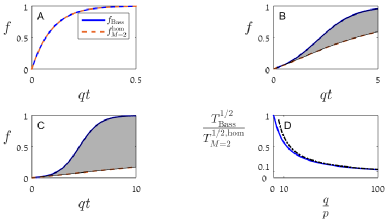
Figure 1: The expected adoption level $f(t)$ of any network ${\cal N}$ lies in the shaded region between the lower bound $f^{\rm hom}_{M=2}$ (orange dash) and upper bound $f_{\rm Bass}$ (blue solid). (A) $\frac{q}{p}=0.1$. The two bounds are nearly indistinguishable. (B) $\frac{q}{p}=10$. (C) $\frac{q}{p}=100$. (D) $\frac{T_{\rm Bass}^{1/2}}{T^{1/2,{\rm hom}}_{M=2}}$ as a function of $\frac{q}{p}$ (blue solid), and its asymptotic approximation (21) (black dashes).

It is instructive to compare the adoption levels on different networks using the “half-life” $T^{1/2}$ for half of the population to adopt. In particular, we can use $T^{1/2}$ to compare the bounds $f_{\rm Bass}$ and $f_{M=2}^{\rm hom}$. The ratio $\frac{T_{\rm Bass}^{1/2}}{T^{1/2,{\rm hom}}_{M=2}}$ can be estimated asymptotically, yielding

$$\frac{T_{\rm Bass}^{1/2}}{T^{1/2,{\rm hom}}_{M=2}}\sim\frac{2}{\log 2}\frac{p}{q}\log\frac{q}{p},\qquad\frac{q}{p}\gg 1.$$ (21)

Figure 1D confirms that $\frac{T^{1/2}_{\rm Bass}}{T^{1/2,{\rm hom}}_{M=2}}$ decreases with $\frac{q}{p}$, and approaches the asymptotic limit (21) as $\frac{q}{p}\rightarrow\infty$. This limit goes to zero as $\frac{q}{p}\rightarrow\infty$, showing that the network structure has a large effect on the diffusion when $\frac{q}{p}\gg 1$, i.e., for products that diffuse primarily by internal influences.

5 Open problems

This manuscript settles the conjecture from [9], but leads to some new questions, which are currently open. Indeed, the upper and lower bounds in Theorems 3 and 5 are tight for networks with any number of nodes. Can these bounds be improved if we restrict ourselves to networks with a fixed number of nodes?

Thus, let

$${\cal G}(p,q,M):=\{{\cal N}\mid\text{${\cal N}$ has $M$ nodes, \eqref{eq:p_j,q_j-homogeneous} holds}\}$$

be the set of all networks with $M$ nodes that are homogeneous in $\{p_{j}\}$ and $\{q_{j}\}$. In the beginning of Section 3.2, we argued that the fastest diffusion in ${\cal G}(p,q,M)$ should occur on the homogeneous complete network (7). Therefore, we formulate

Conjecture 1

$\sup_{{\cal N}\in{\cal G}(p,q,M)}f(t;{\cal N})=f_{\rm complete}(t;p,q,M).$

We note, however, that the rate of convergence of $f_{\rm complete}$ to $f_{\rm Bass}$ as $M\to\infty$ is $O(\frac{1}{M})$, see [11]. Therefore, the difference between these two upper bounds becomes negligible for large (e.g., $M=10^{6}$) networks.

Consider now the lower bound. Let $M$ be even, and let network $\tilde{\cal N}$ be composed of $\frac{M}{2}$ pairs of nodes, each of which is of type ${\cal N}_{M=2}^{\rm hom}$, see (14). Then $f(t;\tilde{\cal N})=f_{M=2}^{\rm hom}(p,q)$. Therefore,

$$\inf_{{\cal N}\in{\cal G}(p,q,M)}f(t;{\cal N})=f_{M=2}^{\rm hom}(p,q),\qquad\text{$M$ even}.$$

Thus, the lower bound $f_{M=2}^{\rm hom}$ cannot be improved (i.e., increased) for networks with a fixed even number of nodes. The tight lower bound for $M$ odd, however, is an open problem.

Another open question is the tight lower bound of $f$ among connected networks with $M$ nodes (even or odd) that are homogeneous in $\{p_{j}\}$ and $\{q_{j}\}$. Here one may need to distinguish between connected undirected networks, weakly-connected directed graphs (there is an undirected path between any pair of vertices), and strongly-connected directed graphs (there is a directed path between every pair of vertices).

6 Proof of results

6.1 Master equations

Denote the nonadoption probability of node $j$ by

$$[S_{j}](t):=1-f_{j}(t)=\mathbb{P}(X_{j}(t)=0).$$ (22)

Then $[S_{j}]$ satisfies the master equation [10]

$$\frac{d}{dt}[S_{j}](t)=-\left(p_{j}+q_{j}\right)\left[S_{j}\right]+\sum_{\begin{subarray}{c}k\in{\cal M}\end{subarray}}q_{k,j}[S_{j},S_{k}](t),\qquad[S_{j}](0)=1,$$ (23)

where $q_{j}$ is given by (4a), and

$$[S_{j},S_{k}](t):=\mathbb{P}(X_{j}(t)=X_{k}(t)=0).$$

In general, to close these equations, one adds the master equations for all pairs $\{[S_{j},S_{k}]\}$, all triplets $\{[S_{j},S_{k},S_{m}]\}$, etc., see [10]. For the purpose of obtaining the lower and upper bounds, however, we will only need the following result:

Lemma 5

Consider the Bass model (3). Then for any $i,j\in{\cal M}$,

$$[S_{i}](t)\,[S_{j}](t)\leq[S_{i},S_{j}](t)\leq e^{-2pt},\qquad 0\leq t<\infty.$$ (24)

Proof 3

The left inequality is proved in [13]. For the right inequality, we note that the joint nonadoption probability of a pair $\{i,j\}$ of isolated nodes ($q_{j}=q_{i}=0$) is given by

$$[S_{i},S_{j}](t;p,q_{j}=q_{i}=0)=e^{-2pt},$$

see, e.g., [14]. Hence, the right inequality follows from Theorem 1.

6.2 Differential and integral Bass inequalities

Let us recall the following result:

Lemma 6 ([9])

Let $p,q>0$, and let $f(t)$ satisfy the differential Bass inequality

$$\frac{df}{dt}<(1-f)(p+qf),\quad t>0,\qquad f(0)=0.$$

Then $f(t)<f_{\rm Bass}(t;p,q)$ for $0<t<\infty$.

Let $[S_{\rm Bass}]:=1-f_{\rm Bass}$ denote the nonadoption level in the compartmental Bass model. Then by (1),

$$\frac{d}{dt}[S_{\rm Bass}](t)=-(p+q)[S_{\rm Bass}]+q[S_{\rm Bass}]^{2},\quad[S_{\rm Bass}](0)=1.$$ (25)

If we replace the equality sign in (25) by an inequality, the solution of this inequality is bounded from below by $[S_{\rm Bass}]$:

Lemma 7

Let $p,q>0$, and let $[S](t)$ satisfies the differential Bass inequality

$$\frac{d}{dt}[S](t)>-(p+q)[S]+q[S]^{2},\quad t>0,\qquad[S](0)=1.$$

Then $[S](t)>[S_{\rm Bass}](t)$ for $0<t<\infty$.

Proof 4

This follows from Lemma 6 and $[S_{\rm Bass}]=1-f_{\rm Bass}$.

Multiplying (25) by $e^{(p+q)t}$, integrating between zero and $t$, and using the initial condition, gives the integral form of the compartmental Bass model

$$[S_{\rm Bass}](t)=e^{-(p+q)t}+q\int_{0}^{t}e^{-(p+q)(t-\tau)}[S_{\rm Bass}]^{2}(\tau)\,d\tau.$$ (26)

If we replace the equality sign in (26) by an inequality, the solution of the resulting integral Bass inequality is bounded from below by $[S_{\rm Bass}]$:

Lemma 8

Let $p,q>0$, and let $[S](t)$ be non-negative and continuous in $[0,\infty)$.

1. If $[S]$ satisfies the integral Bass inequality

   $$[S](t)\geq e^{-(p+q)t}+q\int_{0}^{t}e^{-(p+q)(t-\tau)}[S]^{2}(\tau)\,d\tau,\quad t>0,$$ (27)

   then $[S](t)\geq[S_{\rm Bass}](t;p,q)$ for $t\geq 0$.

2. If inequality (27) is strict, then $[S](t)>[S_{\rm Bass}](t;p,q)$ for $t>0$.

Proof 5

Let $u:=[S]-[S_{\rm Bass}]$. Subtracting (26) from (27) gives

$$u(t)\geq q\int_{0}^{t}e^{-(p+q)(t-\tau)}\left([S]^{2}-[S_{\rm Bass}]^{2}\right)(\tau)\,d\tau.$$

Therefore,

$$u(t)\geq\int_{0}^{t}\phi(\tau)u(\tau)\,d\tau,\qquad\phi(\tau):=qe^{-(p+q)(t-\tau)}\left([S]+[S_{\rm Bass}]\right)(\tau).$$ (28)

Since $[S]$ and $[S_{\rm Bass}]$ are continuous and non-negative, then so is $\phi$. Let

$$v(t):=e^{-\int_{0}^{t}\phi}\int_{0}^{t}\phi(\tau)u(\tau)\,d\tau.$$ (29)

Then $v(0)=0$ and

$$\frac{dv}{dt}=e^{-\int_{0}^{t}\phi}\phi(t)\left(u(t)-\int_{0}^{t}\phi(\tau)u(\tau)\,d\tau\right)\geq 0,$$

where the inequality follows from (28). Therefore, for $t\geq 0$, $v(t)\geq 0$. Hence, by (29), $\int_{0}^{t}\phi(\tau)u(\tau)\,d\tau\geq 0$ and so by (28), $u(t)\geq 0$.

If inequality (27) is strict, we replace in the above proof all “$\geq$” signs by “$>$” signs.

6.3 Upper bound

We begin with an auxiliary result.

Lemma 9

Consider the Bass model (3). Let (19) hold, and let

$$[\underline{S}](t):=\inf_{j\in{\cal M}}\left\{[S_{j}](t)\right\}.$$ (30)

Then $[\underline{S}](t)$ is non-negative and continuous.

Proof 6

The non-negativity of $[\underline{S}]$ follows from that of $\{[S_{j}]\}$. Let $j\in{\cal M}$. Since all probabilities are bounded between $0$ and $1$, then using (23) and (19),

$$\left|\frac{d}{dt}[S_{j}]\right|\leq(p+q)[S_{j}]+\sum_{k\in\cal M}q_{k,j}\left[S_{j},S_{k}\right]\leq p+q+\sum_{k\in\cal M}q_{k,j}\leq\kappa,$$

where $\kappa:=p+2q$. Hence, by the mean-value theorem, for any $t,t^{*}>0$, $\left|[S_{j}](t)-[S_{j}]\left(t^{*}\right)\right|\leq\kappa\left|t-t^{*}\right|$, and so $-[S_{j}]\left(t^{*}\right)\leq-[S_{j}](t)+\kappa\left|t-t^{*}\right|\leq-[\underline{S}](t)+\kappa\left|t-t^{*}\right|$. Taking the supremum of the left-hand side yields $-[\underline{S}]\left(t^{*}\right)\leq-[\underline{S}](t)+\kappa\left|t-t^{*}\right|$, and so $[\underline{S}](t)-[\underline{S}]\left(t^{*}\right)\leq\kappa\left|t-t^{*}\right|$. Swapping $t$ and $t^{*}$ gives the inverse estimate, and so $[\underline{S}](t)$ is continuous.

Proof of Theorem 3. Since $1-f_{m}=[S_{m}]\geq[\underline{S}]$, see (22) and (30), it is sufficient to show that

$$[\underline{S}](t)\geq[S_{\rm Bass}](t,p,q).$$ (31)

By (23) with $q_{j}=q$, see (8),

$$[S_{j}]=e^{-(p+q)t}+\int_{0}^{t}e^{-(p+q)\left(t-\tau\right)}\sum_{k\in\cal M}q_{k,j}\,[S_{j},S_{k}](\tau)\,d\tau.$$ (32)

Therefore, by the lower bound in (24) and (30),

$$[S_{j}]\geq e^{-(p+q)t}+\int_{0}^{t}e^{-(p+q)(t-\tau)}\sum\limits_{k\in\cal M}q_{k,j}\,[S_{j}](\tau)\,[S_{k}](\tau)\,d\tau$$

$$\geq e^{-(p+q)t}+q\int_{0}^{t}e^{-(p+q)(t-\tau)}[\underline{S}]^{2}(\tau)d\tau.$$

Taking the infimum over all $j$ gives

$$[\underline{S}]\geq e^{-(p+q)t}+q\int_{0}^{t}e^{-(p+q)(t-\tau)}[\underline{S}]^{2}(\tau)\,d\tau.$$

Therefore, since $[\underline{S}]$ is non-negative and continuous (Lemma 9), we can use the integral Bass inequality (Lemma 8) to get inequality (31), from which (10) follows. Therefore, by (6), (11) follows. 

Proof of Lemma 3. The result for $f$ follows from Theorem 2. Since the complete network (7) is homogeneous, $f_{m}\equiv f$ for all $m\in\cal M$. Hence, the result holds for any $f_{m}$ as well.

Proof of Theorem 4. Let

$$A_{d}({\cal N}):=\{m\in{\cal M}\mid\text{indegree}\left(m\right)=d\}$$

denote the set of all nodes with indegree $d$ in network ${\cal N}$. Then it is sufficient to prove that for all networks that satisfy (8) and for all $d\in\mathbb{N}$,

$$[S_{m}](t;{\cal N})>[S_{\rm Bass}](t;p,q),\quad t>0,\qquad m\in A_{d}({\cal N}).$$ (33)

We prove (33) by induction on $d$. When $d=0$, node $m\in A_{0}$ is not influenced by any other node, and so

$$[S_{m}](t;{\cal N})=e^{-pt}=[S_{\rm Bass}](t;p,q=0)>[S_{\rm Bass}](t;p,q),$$ (34)

where the inequality follows from Theorem 1.

For the induction stage, we assume that (33) holds for all networks that satisfy (8) and for all $m\in A_{d-1}$, and prove that it holds for all networks that satisfy (8) and for all $m\in A_{d}$, as follows. Let $m\in A_{d}$, where $d\geq 1$, and denote by $\{k_{1},\ldots,k_{d}\}$ the $d$ nodes that can influence $m$. The master equation for $[S_{m}]$ is, see (8) and (23),

$$\frac{d}{dt}[S_{m}]=-(p+q)[S_{m}]+\sum_{i=1}^{d}q_{k_{i},m}[S_{m},S_{k_{i}}],\qquad[S_{m}](0)=1.$$ (35)

By the indifference principle, we can compute each of the $d$ probabilities $\{[S_{m},S_{k_{i}}]\}_{i=1}^{d}$ on a modified network $\widetilde{\cal N}_{i}$, in which we remove the edge $k_{i}\rightarrow{m}$. Thus, $[S_{m},S_{k_{i}}]=\widetilde{[S_{m},S_{k_{i}}]}$, where the tilde sign refers to probabilities in $\widetilde{\cal N}_{i}$. In this modified network, node $m$ has indegree $d-1$, and so by the induction assumption

$$\widetilde{[{S}_{m}]}>[S_{\rm Bass}].$$

In addition, by Theorem 3,

$$\widetilde{[{S}_{k_{i}}]}\geq[S_{\rm Bass}],$$

Combining the above and (24), we have that

$$[S_{m},S_{k_{i}}]=\widetilde{[S_{m},S_{k_{i}}]}\geq\widetilde{[{S}_{m}]}\widetilde{[{S}_{k_{i}}]}>[S_{\rm Bass}]^{2}.$$

Therefore,

$$\sum_{i=1}^{d}q_{k_{i},m}\,[S_{m},S_{k_{i}}]>\sum_{i=1}^{d}q_{k_{i},m}[S_{\rm Bass}]^{2}=q[S_{\rm Bass}]^{2}.$$ (36)

By (35) and (36),

$$\frac{d}{dt}[S_{m}]+(p+q)[S_{m}]>q[S_{\rm Bass}]^{2},\qquad[S_{m}](0)=1.$$

This is the differential Bass inequality (Lemma 6), written in terms of $[S]$, see (7). Hence, $[S_{m}]>[S_{\rm Bass}]$, as needed.

6.4 Lower bound

Proof of Theorem 5. To prove the lower bound (16a) for $f_{m}$, it is sufficient to show that

$$[S_{m}](t)\leq[S_{M=2}^{\rm hom}](t;p,q):=1-f_{M=2}^{\rm hom}(t;p,q)=e^{-pt}\frac{qe^{-pt}-pe^{-qt}}{q-p},$$

where $[S_{m}]=1-f_{m}$. By the upper bound in (24) and (32), we have that

$$[S_{m}]\leq e^{-(p+q)t}+\int_{0}^{t}e^{-(p+q)\left(t-\tau\right)}\sum_{k\in\cal M}q_{k,m}e^{-2p\tau}\,d\tau=e^{-(p+q)t}+q\int_{0}^{t}e^{-(p+q)\left(t-\tau\right)}e^{-2p\tau}\,d\tau$$

$$~{}~{}~{}=\left(1-\frac{q}{q-p}\right)e^{-(p+q)t}+\frac{q}{q-p}e^{-2pt}=\left[S_{M=2}^{\rm hom}\right](t;p,q).$$

Therefore, we proved (16a), which implies (16b).

Proof of Theoren 6 The only inequality in the proof of Theorem 5 arises from using the upper bound in (24). Therefore, the lower bound (16a) for $[S_{m}]$ becomes an equality if and only if $[S_{m},S_{k}]=e^{-2pt}$ for all $k\in{\cal M}\setminus m$ for which $q_{k,m}>0$. A minor modification of Theorem 1 shows that

$$[S_{j},S_{k}]=e^{-2pt}\quad\iff\quad\text{$j$ and $k$ are not influenced by any other node}.$$

Therefore, (17) follows. Since $f=\frac{1}{M}\sum_{j=1}^{M}f_{j}$ for finite networks and $f=\lim_{M\rightarrow\infty}\frac{1}{M}\sum_{j=1}^{M}f_{j}$ for infinite networks, (18) also follows.

Proof of Lemma 4. When $M=2$, this bound is attained by ${\cal N}={\cal N}_{M=2}^{\rm hom}(p,q)$. Moreover, this bound is also attained by any finite or infinite network which is a collection of disjoint pairs of nodes, each of which is of type ${\cal N}_{M=2}^{\rm hom}(p,q)$.

6.5 Asymptotic evaluation of $\frac{T_{\rm Bass}^{1/2}}{T^{1/2,{\rm hom}}_{M=2}}$

By (15), $T^{1/2}:=T_{M=2}^{1/2,{\rm hom}}$ is the solution of

$$e^{-pT^{1/2}}\frac{qe^{-pT^{1/2}}-pe^{-qT^{1/2}}}{q-p}=\frac{1}{2}.$$ (37)

Let $X:=e^{-pT^{1/2}}$ and $\lambda:=\frac{q}{p}$. Then $e^{-qT^{1/2}}=X^{\frac{q}{p}}=X^{\lambda}$. Plugging this into (37), and noting that $0<X<1$ and $\lambda>0$ gives

$$X^{2}-\frac{1}{2}=\frac{p}{q-p}\left(-X^{2}+X^{\lambda}\right)=O\left(\frac{1}{\lambda}\right),\qquad\lambda\gg 1.$$

Therefore,

$$X^{2}\sim\frac{1}{2},\qquad\lambda\gg 1.$$

Hence, by the definition of $X$

$$T^{1/2,{\rm hom}}_{M=2}=\frac{1}{2p}\log(X^{-2})\sim\frac{\log(2)}{2p},\qquad\lambda\gg 1.$$

Finally, by 9, Lemma 11,

$$T_{\rm Bass}^{1/2}=\frac{\log\left(2+\frac{q}{p}\right)}{p+q}\sim\frac{\log\left(\frac{q}{p}\right)}{q},\qquad\lambda\gg 1,$$

and so (21) follows.

References

- Albert et al., [2000] Albert, R., Jeong, H., and Barabási, A. (2000). Error and attack tolerance of complex networks. Nature, 406:378–382.
- Anderson and May, [1992] Anderson, R. and May, R. (1992). Infectious Diseases of Humans. Oxford University Press, Oxford.
- Barabási and Albert, [1999] Barabási, A. and Albert, R. (1999). Emergence of scaling in random networks. Science, 286:509–512.
- Bass, [1969] Bass, F. (1969). A new product growth model for consumer durables. Management science, 15:1215–1227.
- Bollinger and Gillingham, [2012] Bollinger, B. and Gillingham, K. (2012). Peer effects in the diffusion of solar photovoltaic panels. Marketing Science, 31:900–912.
- Delre et al., [2007] Delre, S., Jager, W., Bijmolt, T., and Janssen, M. (2007). Targeting and timing promotional activities: An agent-based model for the takeoff of new products. Journal of business research, 60:826–835.
- Erdős and Rényi, [1960] Erdős, P. and Rényi, A. (1960). On the evolution of random graphs. Publications of the Mathematical Institute of the Hungarian Academy of Sciences, 5:17–60.
- Fibich et al., [2012] Fibich, G., Gavious, A., and Solan, E. (2012). Averaging principle for second-order approximation of heterogeneous models with homogeneous models. Proceedings of the National Academy of Sciences, 109:19545–19550.
- Fibich and Gibori, [2010] Fibich, G. and Gibori, R. (2010). Aggregate diffusion dynamics in agent-based models with a spatial structure. Operations Research, 58:1450–1468.
- Fibich and Golan, [2022] Fibich, G. and Golan, A. (2022). Diffusion of new products with heterogeneous consumers. Mathematics of Operations Research.
- Fibich et al., [2023] Fibich, G., Golan, A., and Schochet, S. (2023). Compartmental limit of discrete Bass models on networks. Discrete and Continuous Dynamical Systems - B, 28:3052–3078.
- [12] Fibich, G., Golan, A., and Schochet, S. (Preprint). Monotone convergence of discrete Bass models.
- [13] Fibich, G. and Levin, T. (Preprint). Funnel theorems for spreading on networks. available at http://arxiv.org/abs/2308.13034.
- Fibich et al., [2019] Fibich, G., Levin, T., and Yakir, O. (2019). Boundary effects in the discrete bass model. SIAM Journal on Applied Mathematics, 79:914–737.
- Garber et al., [2004] Garber, T., Goldenberg, J., Libai, B., and Muller, E. (2004). From density to destiny: Using spatial dimension of sales data for early prediction of new product success. Marketing Science, 23:419–428.
- Garcia, [2005] Garcia, R. (2005). Uses of agent-based modeling in innovation/new product development research. Journal of Product Innovation Management, 22:380–398.
- Goldenberg et al., [2001] Goldenberg, J., Libai, B., and Muller, E. (2001). Using complex systems analysis to advance marketing theory development. (special issue on emergent and co-evolutionary processes in marketing.). Acad. Market. Sci. Rev., 9:1–19.
- Goldenberg et al., [2010] Goldenberg, J., Libai, B., and Muller, E. (2010). The chilling effects of network externalities. International Journal of Research in Marketing, 27:4–15.
- Goldenberg et al., [2008] Goldenberg, J., Lowengart, O., and Shapira, D. (2008). Zooming in: Self-emergence of movements in new product growth. Marketing Science, 28:274–292.
- Graziano and Gillingham, [2015] Graziano, M. and Gillingham, K. (2015). Spatial patterns of solar photovoltaic system adoption: The influence of neighbors and the built environment. Journal of Economic Geography, 15:815–839.
- Hopp, [2004] Hopp, W. (2004). Ten most influential papers of management science’s first fifty years. Management Science, 50:1763–1764.
- Jackson, [2008] Jackson, M. (2008). Social and Economic Networks. Princeton University Press, Princeton and Oxford.
- Kiss et al., [2017] Kiss, I., Miller, J., and Simon, P. (2017). Mathematics of epidemics on networks. Springer.
- Mahajan et al., [1993] Mahajan, V., Muller, E., and Bass, F. (1993). New-product diffusion models. Handbooks in operations research and management science, 5:349–408.
- Muller and Peres, [2019] Muller, E. and Peres, R. (2019). The effect of social networks structure on innovation performance: A review and directions for research. International Journal of Research in Marketing, 36:3–19.
- Niu, [2002] Niu, S. (2002). A stochastic formulation of the Bass model of new product diffusion. Mathematical problems in Engineering, 8:249–263.
- Pastor-Satorras and Vespignani, [2001] Pastor-Satorras, R. and Vespignani, A. (2001). Epidemic spreading in scale-free networks. Physical review letters, 86:3200–3203.
- Peres, [2014] Peres, R. (2014). The impact of network characteristics on the diffusion of innovations. Physica A, 402:330–343.
- Rand and Rust, [2011] Rand, W. and Rust, R. (2011). Agent-based modeling in marketing: Guidelines for rigor. International Journal of research in Marketing, 28:181–193.
- Scellato et al., [2011] Scellato, S., Noulas, A., Lambiotte, R., and Mascolo, C. (2011). Socio-spatial properties of online location-based social networks. In Proceedings of the International AAAI Conference on Web and Social Media, volume 5, pages 329–336.
- Strang and Soule, [1998] Strang, D. and Soule, S. (1998). Diffusion in organizations and social movements: From hybrid corn to poison pills. Annual review of sociology, 24:265–290.
- Watts and Strogatz, [1998] Watts, D. and Strogatz, S. (1998). Collective dynamics of ‘small-world’ networks. Nature, 393:440–442.