Shock induced ignition and transition to detonation in the presence of mechanically induced non-linear acoustic forcing

Abstract

We address the problem of shock induced ignition and transition to detonation in a reactive medium in the presence of mechanically induced fluctuations by a moving oscillating piston. For the inert problem prior to ignition, we provide a closed form model for the generation of the train of compression and expansions, their steepening into a train of N-shock waves and their reflection on the lead shock, as well as the distribution energy dissipation rate in the induction zone. The model is found in excellent agreement with numerics. Reactive calculations were performed for hydrogen and ethylene fuels using a novel high-fidelity numerical Lagrangian scheme. Different regimes of ignition and transition to detonation, controlled by the time scale of the forcing and the two time scales of the chemistry: the induction and reaction times. Two novel hot spot cascade mechanisms were identified. The first relies on the coherence between the sequence of hot spot formation set by the piston forcing and forward wave interaction with the lead shock, generalizing the classic runaway in fast flames. The second hot spot cascade is triggered by the feedback between the pressure pulse generated by the first generation hot spot cascade and the shock. For slow forcing, the sensitization is through a modification to the classic run-away process, while the high frequency regime leads to very localized sub-critical hot-spot formation controlled by the cumulative energy dissipation of the first generation shocks at a distance comparable to the shock formation location.

1 Introduction

The process of deflagration to detonation transition (DDT) is central to both astrophysical reactive hydrodynamics, as it controls, for example, Supernovae explosions of white dwarfs, and terrestrial reactive hydrodynamics, as flames, given sufficient development time and appropriate boundary conditions, will eventually accelerate their volumetric burning rate until forming detonations. Detonations in reactive gases propagate at hypersonic speeds, with Mach numbers ranging from 5 to 8 and overpressures in the range of 10 to 20. Clearly, the transition phenomenon is to be avoided in the process industries, but can be beneficial in propulsion applications utilizing the tremendous power of detonation waves, such as pulse detonation, oblique detonation and rotating detonation engines.

The transition from deflagration to detonation is marked by a continuous switch in ignition mechanism. While in deflagrations, ignition is controlled mainly by diffusion of active species and energy, in detonations, diffusionless auto-ignition relying on gas compression by waves is the main driving mechanism. The transition from deflagrations to detonations is a three-dimensional phenomenon, and involves the deformation of the flame surface area by non-homogeneous flow, and even disruption of the flamelet structures themselves, when active turbulent time scales are shorter than those of flames. Reviews of DDT phenomena can be found in the work of Lee & Moen (1980), Ciccarelli & Dorofeev (2008), with an entry point in the more modern literature in the more recent work of Poludnenko et al. (2019), Oran et al. (2020), Saif et al. (2017) and Bychkov et al. (2012) and their co-workers.

The last stages of DDT generally occur when the volumetric burning rate averaged at some macro-scale associated with the front definition and propagation attains the maximum value permitting steady propagation, denoted by the Chapman-Jouguet condition (Eder & Brehm, 2001; Dorofeev et al., 2000; Chue et al., 1993; Poludnenko et al., 2019; Saif et al., 2017). In practice, depending on boundary conditions, this CJ deflagration is invariably headed by a shock wave (Rakotoarison et al., 2024). An example of the last stages of DDT is shown in Fig. 1. At this stage, the flame acts like a fast piston, sustaining the lead shock. Any acceleration in global burning rate at this stage does not permit quasi-steady propagation and translates into the generation of a train of forward and rear facing shocks. The DDT process is the series of rapid auto-ignition phenomena that collectively yield a detonation wave. Experiments and numerical simulations of DDT are usually very difficult to re-construct and rationalize due to this inherent multi-scale and multi-dimensional phenomenon. This is usually compounded by the fact that hot spot ignition is influenced in a non-trivial way by other neighbouring hot-spots, and their interaction is mainly gas dynamic, i.e., via compression and expansion waves that can be long-ranged.

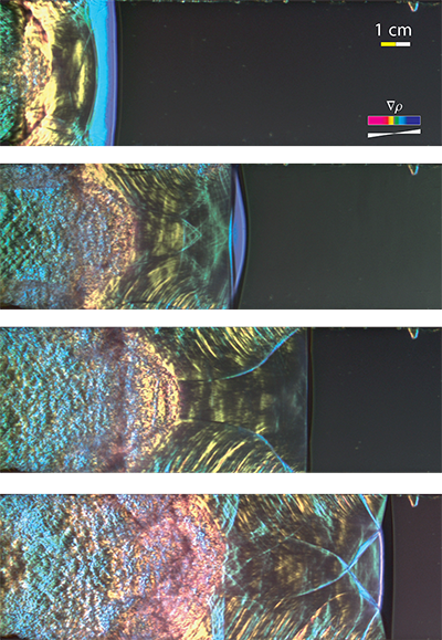
Figure 1: The propagation of a Chapman-Jouguet deflagration wave headed by a shock and the subsequent detonation formation in H₂-air, $\phi=0.65$, illustrating the pressure waves emitted by the non-planar flame and DDT ahead of the flame in the last frame; adapted from Eder (2001).

DDT onset is also quite difficult to predict in engineering calculations that only assess the global flame dynamics and lead shock strength. DDT is usually a sub-grid phenomenon to be modelled (Dorofeev et al., 2000; Middha & Hansen, 2008). For example, Meyer et al. (1970) have shown that the detailed reconstruction of the global dynamics (i.e., space and time filtered) of the lead shock is insufficient to predict the DDT. More recently, Saif et al. (2017) showed that the ignition delays calculated for the mean lead shock speed measured experimentally over-predict the real ignition and DDT time scales observed in the experiments by several orders of magnitude in sensitive mixtures. It is well recognized that this discrepancy is due to fine scale events and hot-spot formations, that can be formed by a variety of mechanisms (Saif et al., 2017; Oran & Gamezo, 2007). This calls for a multiple hot-spot model for DDT, which is the main motivation of the present study.

The existing theory of DDT is currently restricted to the formation of single reactive spots in which auto-ignition occurs. The coupling between the gas-dynamic evolution and the chemical dynamics controlling the ignition delays is now well understood. It can explain the vast type of behaviour depending on the sensitivity of the induction kinetics to temperature release, initial gradients in fluid state, and time scales of energy deposition. Reactive front propagation is conditioned by the local ignition time gradients. Much of the work focuses on the coupling of the so-called fast, or diffusionless flames, and the gasdynamics fields, which controls pressure wave amplification. This is a modern extension of the Zel’dovich gradient mechanism that exploits the coherence between the speed of fast flames, controlled by reactivity gradients and acoustic waves. This coherence extends to shock waves as well, and is sometimes called Shock Wave Amplification by Coherent Energy Release (SWACER) (Lee & Moen, 1980). An entry point in the vast modern literature on the subject is the lucid treatment of Sharpe & Short (2003).

The present study aims to bridge the local dynamics of hot spot runaway and the dynamics of real turbulent flames, in which cooperative phenomena between multiple hotspots is likely to give rise to emergent phenomena. We thus reduce the dimensionality of the problem to 1D, and consider a non-steady piston, modelling the flame, that generates mechanical disturbances in the medium ahead of it, in the form of compression and expansion waves. These waves not only modify the state of the gas ahead of the piston directly, but also interact with the lead shock, generating entropy layers. The resulting non homogeneous reactive field is then conducive to multiple hot-spot formation and transition to detonation. The control parameters are the strength of the lead shock, controlled by the mean piston speed and the amplitude and frequency of the mechanical waves, controlled by the piston’s speed fluctuations and frequency. In spite of the model’s apparent simplicity, it will be shown numerically and analytically, that different ignition and DDT regimes can be observed, with sometimes profound consequences on the time scales of ignition and DDT and how they differ from calculations without account of perturbations.

For physical clarity and computational efficiency, the problem is posed in Lagrangian coordinates, such that particle paths are easily tracked and visualized and numerical diffusion usually plaguing this type of numerical calculations can be controlled. A novel numerical scheme is formulated. We first study the non-steady gasdynamics that arise in a non-reactive medium, treating the problem numerically and theoretically in the weakly non-linear acoustic regime. The temperature field obtained then serves as leading order solution for investigating and interpreting the reactive dynamics. The reactive dynamics are determined numerically. We focus on two fuel mixtures, H₂-O₂ and C₂H₄-O₂, with realistic chemistry to highlight the importance of the different ignition and reaction time scales, as well as the sensitivity of ignition delay to temperature.

The paper is organized as follows. Section 2 provides the statement of the physical model and governing equations for a reactive diffusionless fluid in Lagrangian coordinates, while a derivation is given in the appendix A. Section 3 details the new formulation of a numerical scheme and its validation. Section 4 provides the solution to the inert problem. Section 5 provides the results of reactive calculations for the two fuels. Section 6 discusses the various regimes of ignition and DDT in terms of the amplitude and frequency of the forcing.

2 Problem definition in Lagrangian coordinates

The one-dimensional problem is illustrated schematically in Fig. 2 in the laboratory, or Eulerian frame, as well as in the Lagrangian frame of reference following particle paths. A piston is set in motion at time $t=0$ into a gas at rest and of homogeneous state denoted by a subscript ”0”. The piston has a non steady speed given by

$$u_{p}=u_{p0}+A\sin(2\pi ft)$$ (1)

where $u_{p0}$, $A$ and $f$ represent the average speed, fluctuation amplitude and fluctuation frequency respectively. These are held constant. It means the piston motion is modelled as a constant speed motion to which is superimposed a simple harmonic motion (SHM). In current problem, SHM is considered as the fluctuation, i.e., $A\ll u_{p0}$.

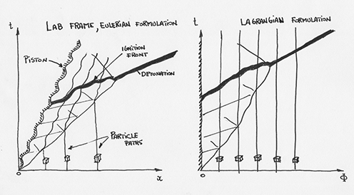
Figure 2: Schematic of the problem solved in the Eulerian and Lagrangian frame of reference, in which the particle label $\phi$ serves as independent variable replacing the space variable $x$.

The piston’s impulsive motion generates a main lead shock, followed by a non-homogeneous state affected by the piston fluctuations. These fluctuations are controlled by the compression/expansion waves originating at the piston, interactions of these with the lead shock, generation of entropy waves along particle paths and of course internal and rear boundary and lead shock reflections of these waves.

The problem can be posed in Lagrangian coordinates. A general derivation starting from the more familiar Eulerian formulation is presented in the Appendix A. The field equations are

$$\frac{\partial v}{\partial t}-\frac{\partial u}{\partial\phi}=0$$ (2)

$$\frac{\partial u}{\partial t}+\frac{\partial p}{\partial\phi}=0$$ (3)

$$\frac{\partial e_{tot}}{\partial t}+\frac{\partial pu}{\partial\phi}=0$$ (4)

$$\frac{\partial Y_{i}}{\partial t}=v\omega_{i}$$ (5)

where $v=1/\rho$ is the specific volume, $u$ the particle speed, $p$ the pressure, $e_{tot}=e+\frac{1}{2}u^{2}$ is the total energy, $e=\sum\limits_{i=1}^{N}Y_{i}e_{i}$ the specific internal energy of the mixture, $Y_{i}$ the mass fraction of the i${}^{\text{th}}$ component and $\omega_{i}$ the mass production rate of specie $i$ per unit volume, per unit time, obtained from chemical kinetics. The independent variables are time $t$ and a mass weighted Lagrangian coordinate $\phi$, defined in terms of the Eulerian space variable $x$ by

$$\phi=\int_{x_{p}(t)}^{x}\rho\mathrm{d}x$$ (6)

where $x_{p}(t)$ is the trajectory of the piston in the laboratory frame. A line of constant $\phi$ denotes a particle path.

These equations are supplemented by the equation of state for an ideal gas linking the dependent variables to the mixture temperature $T$ and the prescription of $\omega_{i}$, the mass production rate of specie $i$ per unit volume per unit time and $e_{i}$ in terms of the field variables from a thermo-kinetic database. This formulation is standard and not reproduced here; see for example Kee et al. (2005). In the present study, the real gas thermo-chemical properties of the mixture required for prescribing $\omega_{i}$ and $e_{i}$ in terms of the field variables are obtained using the Li et al. (2004) thermochemical database for the calculations involving hydrogen and the reduced San Diego thermo-chemical database for the ethylene calculations (Varatharajan & Williams, 2002a, b).

3 Numerical method

Both reactive and inert calculations require the numerical solution of the Lagrangian conservation laws given by (2) to (5). We note these are written in conservation form

$$\frac{\partial U}{\partial t}+\frac{\partial\mathcal{F}}{\partial\phi}=Q$$ (7)

with ”conserved” variables $U=\left[v,u,e_{tot},Y_{i}\right]^{T}$, corresponding ”fluxes” $\mathcal{F}=\left[-u,p,pu,0\right]^{T}$ and sources $\mathcal{F}=\left[0,0,0,v\omega_{i}\right]^{T}$. Standard finite volume methods for compressible flow apply, here the volume being a mass element. While the equivalent modern finite volume methods for hyperbolic system of equations have been demonstrated for Lagrangian coordinates, e.g., (Munz, 1994), we are not aware of their application to reactive flows. Our extension of these methods to reactive flows is the well established operator splitting method of treating sequentially the inert hydrodynamics and the reactive problems (LeVeque et al., 2002), usually used in solving the Eulerian system of gas-dynamics. This operator-splitting approach is particularly attractive in the Lagrangian system, as no mass is transferred between the neighbour elements. Each volume contains the same gas through out the entire simulation, which minimizes numerical diffusion errors. Each element of gas responds solely to compression/expansion from neighbouring ones. While the inert hydrodynamic solver, detailed next, follows current best practices for high order resolution of gas dynamic discontinuities, the reactive step uses the Cantera package to integrate the resulting ordinary differential equations with their build-in stiff ODE solver (Goodwin & Moffat, 2017).

3.1 Hydrodynamics

The hydrodynamic step uses a second order HLLE scheme devised for a structured uniform grid in the $\phi$ dimension, as shown schematically in Fig. 3. The solution vector for $U$ is stored at the cell centres and the fluxes are evaluated at the cell interfaces. The solution inside one of these cells is represented by piecewise limited linear functions. Central differences are used to reconstruct the slopes and van Albada limiter (Van Albada et al., 1997) has been applied to limit variations in conserved variables. The cell-averaged values of the conserved quantities $U_{i}$ are updated by computing the flux at the two numerical cell interfaces $\mathcal{F}_{i-1/2}$ and $\mathcal{F}_{i+1/2}$, where $i$ is the index of cells. The inter-cell flux $\mathcal{F}$ is evaluated through the approximation solver of the Riemann problem using the HLLE flux functions with the reconstructed left and right state at the cell boundary described by Einfeldt et al. (1991). The left and right states are interpolated values at the cell of the left and right side of the cell interface. The second order spatial-temporal step is performed as follows. First a first-order approximation is obtained:

$$\hat{\bar{U}}_{i}^{n+1}=\bar{U}_{i}^{n}+\dfrac{\Delta t}{\Delta x}\left[\mathcal{F}_{i+1/2}^{n}-\mathcal{F}_{i-1/2}^{n}\right]$$ (8)

This solution $\hat{\bar{U}}_{i}^{n+1}$, together with the initial vector $\bar{U}_{i}^{n}$ are then used to update the second-order cell state $\widetilde{U}_{i}^{n+1}$ according to

$$\widetilde{U}_{i}^{n+1}=\bar{U}_{i}^{n}+\dfrac{\Delta t}{2\Delta x}\left[\mathcal{F}_{i+1/2}^{n}+\hat{\mathcal{F}}_{i+1/2}^{n}-\mathcal{F}_{i-1/2}^{n}-\hat{\mathcal{F}}_{i-1/2}^{n}\right]$$ (9)

For the inert problem, this is the final solution after one time step, i.e., $\bar{U}_{i}^{n+1}$. When the reactions are coupled, $\widetilde{\bar{U}}_{i}^{n+1}$ is further updated after the reaction step. During the hydrodynamic substep, the ideal gas law is used with an isentropic coefficient, $\gamma$, provided by Cantera at the end of the last chemical sub-step. The local value of $\gamma$ is assumed constant during a hydrodynamic step.

The boundary $\phi=0$ corresponds to the piston face, where the gas speed is that of the piston. In order to impose a flux into the first cell, the pressure is determined by solving the exact Riemann problem with the velocity of the piston at the cell boundary. Once the velocity and the pressure is evaluated in the cell boundary, the flux can be prescribed. The boundary condition at the right boundary of the computational domain uses an extrapolation of cubic interpolation; nevertheless, the calculation ends before the lead shock reaches the right boundary such that this local boundary condition does not have any role in the calculation.

Figure 3: At a given time, the solution in neighbouring cell mass elements is represented by piece-wise linear functions used to achieve second order accuracy in the solution of the Riemann problem at cell interfaces for calculating inter-cell fluxes.

3.2 Chemical species evolution

The second sub-step in the operator-splitting scheme is to advance the chemical composition in each cell while maintaining the density, speed and total internal energy constant in each cell. This is equivalent to evolving the species concentrations at fixed internal energy and constant volume. This calculation is performed using Cantera’s computational framework already available for this canonical calculation. Each cell has been treated as a constant-volume closed reactor in Cantera during the chemical reaction step. The ODE’s are solved using the SUNDIALS stiff ODE solver used by Cantera over the global time step $\Delta t$ dictated by the hydrodynamics. At the end of each chemical step, the pressure and isentropic coefficient has been updated and sent back to the hydrodynamic solver. The mass fractions of all reacting components remains frozen during the subsequent hydrodynamic step.

3.3 Numerical verification

3.3.1 Verification of the hydrodynamic solver

Two frozen hydrodynamic problems have been chosen to verify the correct implementation of the hydrodynamic solver and confirm the adequacy of the numerical method proposed. The first problem is a Riemann problem involving a weak shock and expansion fan in a perfect gas. An initial discontinuity at $x=1$ separates the left state $\left(u_{l}=0,p_{l}=2,\rho_{l}=1\right)$ from the right state $\left(u_{r}=0,p_{r}=1,\rho_{r}=0.5\right)$ with the isentropic coefficient $\gamma=1.4$ constant for both sides. Figure 4 shows the comparison of the calculated density with the exact solution at time $t=0.3$. It is found that the numerical scheme treats satisfactorily the shock, contact surface and expansion wave typical of the HLLE scheme.

The second test problem is a strong shock case in a real gas, with frozen chemical composition. A piston with a constant speed of 1500m/s moves into a stoichiometric mixture of hydrogen and oxygen at pressure $p_{r}=101325$Pa and temperature $T_{r}=293$K. Figure 4 shows the comparison of the calculated density with the exact solution at time $t=0.03$s, where excellent agreement is observed between the computed and the exact solution. This confirms the reliability of the numerical solver.

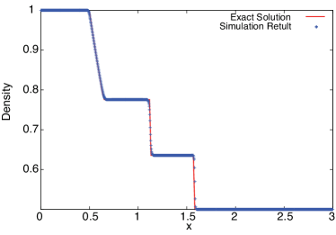
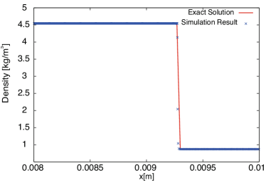
Figure 4: Density profile for shock-expansion problem(left); strong shock problem(right)

3.3.2 Verification of the reactive solver coupling to hydrodynamics

The coupling between the reactive and hydrodynamic solver was tested in the stable detonation wave propagation. The test is whether the solver can propagate a stable ZND detonation wave. We tested an over-driven ZND detonation in a stoichiometric mixture of hydrogen and oxygen initially at $1.01\times 10^{5}$ Pa and 300 K. A piston speed of 2583.6 m/s drives a detonation wave propagating at 3500 m/s. The calculation was initialized with the ZND detonation profile calculated separately using the Shock and Detonation Toolbox in Cantera. Figure 5 shows the evolved wave structure at $t=4.8\times 10^{-7}$s. The calculation used a CFL number is 0.7. Excellent agreement is found between the calculated detonation structure and the expected travelling wave solution provided by the ZND solution, verifying the numerical coupling between the reactive and hydrodynamic solvers.

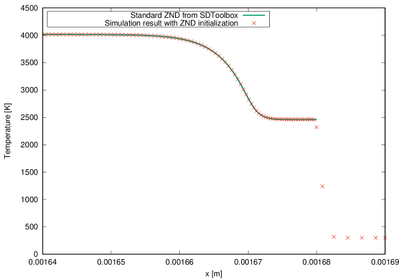
Figure 5: Temperature profile for the ZND test

4 The inert problem solution in the induction zone

4.1 Overview

The ignition of the gas induced by the lead shock in the presence of gasdynamic fluctuations is controlled by the temperature and pressure variation in the induction zone, prior to the onset of exothermicity. It is thus useful to establish the fluctuations induced by the piston first, without account for exothermicity.

A numerical example of the temperature evolution in the induction zone is illustrated in the $\phi-t$ diagram of Fig. 6 by freezing the exothermicity. The mixture is $2H_{2}+O_{2}$ initially at $T_{0}=300$K and $p_{0}=5.90\times 10^{3}$Pa, with a mean piston speed $u_{p0}=1.63\times 10^{3}$m/s, fluctuation amplitude $A=0.2u_{0}$ and frequency of $f=45.4$kHz. This leads to a non-fluctuated post-shock temperature $T_{1}=1100K$ and post-shock pressure $p_{1}=1$Atm. The reactive solution to this problem is discussed later.

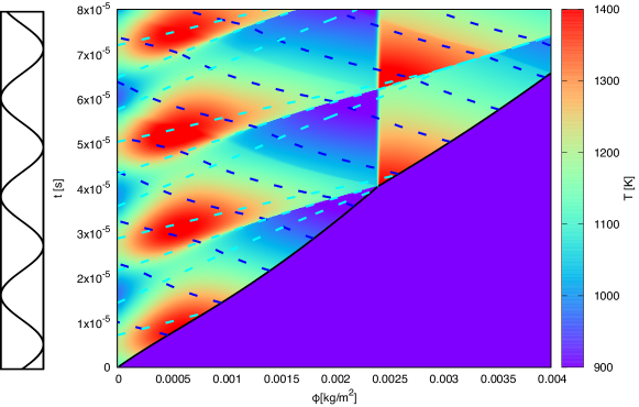
Figure 6: Temperature evolution in $\phi-t$ space induced by the impulsive piston motion ($u_{0}=1626.35$m/s, $A=0.2u_{p0}$ and $f=45.4$ kHz) into chemically frozen $2H_{2}+O_{2}$ initially at $T_{0}=300$K and $p_{0}=5900$ Pa; dark dashed blue lines are C- characteristics while cyan dashed blue lines are C+ characteristics.

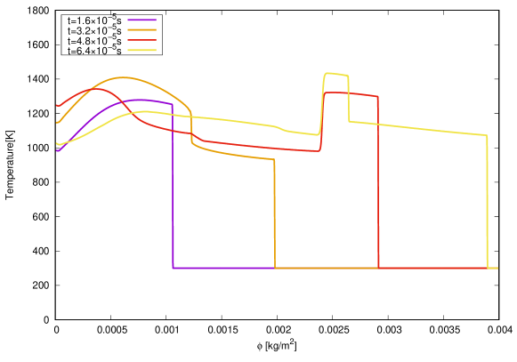
Figure 7: Temperature profiles at several times; same conditions as Fig. 6.

While the impulsive piston motion generates instantly a lead shock, the subsequent compressive parts of the piston motion generate a waveform that steepens to form internal shocks. These internal shocks can be readily identified as right facing fronts. This forward facing waveform then reflects on the lead shock, generating reflected disturbances along the C- characteristics and along (vertical) particle paths. One of these evident entropy waves can be identified as originating at the lead shock when an internal shock wave overtook the lead shock at approximately $t=3.8\times 10^{-5}$s. The particle path evolution can thus be seen to be modulated by the initial temperature obtained at the shock and the subsequent isentropic expansion or compression in regions sufficiently close to the piston before inner shock formation, or further wave by inner shock heating.

The magnitude and wave shape of the fluctuations can also be observed in Figure 7, which shows the temperature distributions at four different times. The last profile corresponds to an instant just prior of the lead shock arrival at the right boundary of the computational domain in this case. Inner shocks and contact surfaces discussed above can be clearly identified. Note, however, that it would have been very difficult to rationalize these features without the space-time diagram illustrating the wave dynamics.

Given the propensity to form inner shocks and their role in shock heating the gas in the induction zone, it is desirable to construct an approximate analytical model for the process to predict the timing of the various events and the temperature amplitude. The problem can be conceptualized as follows. The state generated by an impulsively started steadily moving piston (state 1) behind a constant speed shock can be taken as the leading order constant solution. Perturbations to this state are brought about by the harmonic piston motion. Denoting the overpressure of the lead shock as $z_{1}=(p_{1}-p_{0})/p_{0}$, the Riemann variable $J^{-}$ across the shock varies as $O(z_{1}^{3})$ while pressure, density and speed vary as $O(z_{1})$ (the acoustic solution) (Chandrasekhar, 1943; Whitham, 1974). A weakly non-linear description of the state evolution behind the lead shock can thus be sought assuming $J^{-}=const.$ to order $O(z_{1}^{2})$. This constitutes a ”simple wave” solution first suggested by Chandrasekhar (1943) and further exploited by Whitham (1974) in different shock formation problems. This is the first inert problem to which we seek a simple solution, labelled problem A. Its weak non-linearity permits to account for the dynamics of inner shock waves.

The problem B we wish to solve is the interaction of right facing waves described in problem A, with the lead shock, which leads to reflected waves along particle paths and C- characteristics. This reflection problem is solved in the linear regime and serves to correct the lead shock strength and the interior states provided by problem A.

We thus seek solutions of the form:

$$u=u_{1}+u_{A}+u_{B}...$$ (10)

$$p=p_{1}+p_{A}+p_{B}...$$ (11)

$$T=T_{1}+T_{A}+T_{B}...$$ (12)

4.2 Problem 0: The constant speed shock driven by the steady piston

The leading order solution is the shock driven by the impulsively started piston at steady speed $u_{p0}$ into quiescent gas at state 0. This generates a constant state between the piston and the lead shock labelled with subscript 1, which obeys the usual Rankine-Hugoniot shock jump conditions.

4.3 Problem A: right facing wave train and inner shock formation

The piston speed departure from the steady state $u_{A}(\phi=0)=u_{p}-u_{p0}=A\sin(2\pi ft)$ generates a train of waves propagating into the gas at state 1. The weakly non-linear waveform generated by an oscillating piston behind the lead shock can be obtained by neglecting $O(z^{3})$ variations in entropy and $J^{-}$ Riemann variable across the lead shock and all internal shocks. This simple wave problem is solved in closed form in Lagrangian coordinates for a perfect gas. We are not aware of its solution elsewhere, although similar arguments were presented by Chandrasekhar (1943) and Whitham (1974) in other problems in Eulerian coordinates, which makes the analysis more complicated.

As detailed in the Appendix, the characteristic equations for isentropic flow of a perfect gas are

$$\frac{\partial J^{\pm}}{\partial t}\pm\rho c\frac{\partial J^{\pm}}{\partial\phi}=0$$ (13)

where the Riemann variables are $J^{\pm}=2c/(\gamma-1)\pm u$. Since all C- characteristics originate from the upstream state 0, $J^{-}=J^{-}_{1}=J^{-}_{0}$ is constant everywhere to the level of the current approximation and we have immediately the simple wave relation between flow and sound speed perturbations:

$$c=c_{1}+(u-u_{1})\frac{\gamma-1}{2}$$ (14)

Given the flow is isentropic in the current approximation, all variables can be related to the sound speed variation

$$\frac{\rho}{\rho_{1}}=\left(\frac{p}{p_{1}}\right)^{\frac{1}{\gamma}}=\left(\frac{T}{T_{1}}\right)^{\frac{1}{\gamma-1}}=\left(\frac{c}{c_{1}}\right)^{\frac{2}{\gamma-1}}$$ (15)

and using (14), the propagation speed of forward facing characteristics in the $\phi-t$ can be expressed in terms of $u$ only.

$$\frac{d\phi}{dt}=\rho c=\rho_{1}c_{1}\left(1+\frac{u-u_{1}}{c_{1}}\frac{\gamma-1}{2}\right)^{\frac{\gamma+1}{\gamma-1}}$$ (16)

Similarly, using (14), the Riemann variable $J^{+}$ can also be expressed in terms of $u$ only. Given $J^{+}$ remains constant along C+ characteristics, it implies that $u$ remains constant along C+ characteristics (and all other variables by virtue of (14) and (15)) and C+ characteristics are straight lines. These characteristics hence communicate the values of $u$, $c$, $\rho$, $\rho c$,$T$, $p$, etc. from the piston face forward. In short, all variables hence satisfy the simple advection equation for $\alpha=u,c,\rho,\rho c,T,p...$,

$$\frac{\partial\alpha}{\partial t}+\rho_{1}c_{1}\left(1+\frac{u-u_{1}}{c_{1}}\frac{\gamma-1}{2}\right)^{\frac{\gamma+1}{\gamma-1}}\frac{\partial\alpha}{\partial\phi}=0$$ (17)

The trajectory of any C+ characteristic can be obtained by integrating (16) from the piston $\phi=0$ and reference time $t^{*}$, yielding

$$\phi=\rho_{1}c_{1}\left(1+\frac{u(t^{*})-u_{1}}{c_{1}}\frac{\gamma-1}{2}\right)^{\frac{\gamma+1}{\gamma-1}}(t-t^{*})$$ (18)

Since $u(t^{*})$ is the piston speed, this expression provides implicitly the dependence $t^{*}(\phi,t)$. Given $t^{*}$, $u(t^{*})$ is known and remains constant along that characteristic. The other variables are obtained from (14) and isentropic relations (15). Using the harmonic piston speed perturbation, (18) can be written as

$$\phi=\rho_{1}c_{1}\left(1+\frac{A\sin(2\pi ft^{*})}{c_{1}}\frac{\gamma-1}{2}\right)^{\frac{\gamma+1}{\gamma-1}}(t-t^{*})$$ (19)

which can be further simplified for small Mach number harmonic motion or in the Newtonian limit $\gamma\rightarrow 1$ to

$$\phi=\rho_{1}c_{1}\left(1+\frac{\gamma+1}{2}\frac{A\sin(2\pi ft^{*})}{c_{1}}\right)(t-t^{*})$$ (20)

The solution is complete but breaks down when characteristics intersect and the solution becomes multi-valued. When this happens, shocks need to be fitted. The shock formation time and location, as well as the fitted inner shock trajectories can be obtained in closed form.

Figure 8 illustrates the shock formation and the fitted shock trajectory, which approximately bisects the angle formed by the characteristics originating from either side of the shock. Shocks will form along the characteristics where the front was initially steepest at the piston face, i.e. $d(\rho c)/dt$ was initially maximum, since these steepest points on the waveform will be maintained on the same characteristic. At the piston face, we have

$$\rho c=\rho_{1}c_{1}\left(1+\frac{\gamma+1}{2}\frac{A\sin(2\pi ft^{*})}{c_{1}}\right)$$ (21)

and the steepest points are located at $t=t_{X}=n/f$ with $n=0,1,2,3....$. Shocks will thus form along these characteristics, which are given by

$$(\rho c)_{X}=\rho_{1}c_{1}=\frac{\phi}{t-t_{X}}$$ (22)

These characteristics will intersect with a neighbouring characteristic originating at point $\phi=0$ and $t=t_{X}+\delta t$ and having a propagation speed $(\rho c)_{X}+\frac{d\rho c}{dt}\delta t$ at the shock formation time

$$t^{*}=\frac{n}{f}+\frac{1}{(\gamma+1)\pi fA/c_{1}}$$ (23)

and shock formation particle label

$$\phi^{*}=\frac{\rho_{1}c_{1}}{(\gamma+1)\pi fA/c_{1}}$$ (24)

in the limit of $\delta_{t}\rightarrow 0$. For the example considered, the shock is predicted to form at particle label $\phi^{*}=1.26\times 10^{-3}$kg/m², in very good agreement with the simulations shown in Fig. 9.

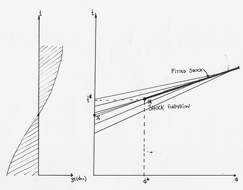
Figure 8: Sketch illustrating the shock formation process along the characteristic passing through the point where $\rho c$ had the steepest rate of increase on the piston face (point X); shock forms at point * from characteristics merging.

The fitted shock trajectory can be approximated to be the continuation of the characteristic along which the shock has first formed. This approximation is the leading order solution for weak shocks (Whitham, 1974), since the speed of weak shocks is the average of the speed of the characteristics on either side. It can be shown that the error in shock position location in this case is given by the square of the characteristic speed perturbation, i.e. $\left(\frac{\rho c-\rho_{1}c_{1}}{\rho_{1}c_{1}}\right)^{2}$. This is a higher order effect than the simplification leading to (20), hence can be neglected. The analytical solution is now complete.

Figure 9 shows the prediction of the wave dynamics obtained numerically by the full hydrodynamic numerical solution and its comparison with the analytical prediction developed above. Select profiles are shown in Fig. 10. The analytical solution is found in very good agreement with the numerics, in spite of the various simplifications made. The analytical prediction nevertheless somewhat under-predicts the exact numerical solution once the inner shocks are formed. The reason is that the inner shock waves keep dissipating the heat to the local gas during the propagation. Although such heat is small comparing to the fluctuation energy, this mechanism is irreversible and will continuously heat the gas. Before the inner shocks form, this dissipation is negligible and the agreement between numerics and the analytical result is very good.

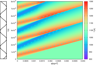
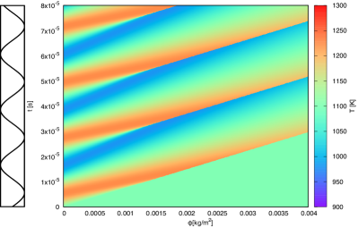
Figure 9: Temperature evolution in chemically frozen $2H_{2}$+$O_{2}$ initally at $T_{1}=1100$K generated by a piston speed with fluctuation amplitude $A=325.27$m/s; numerical result (left) and analytical prediction (right).

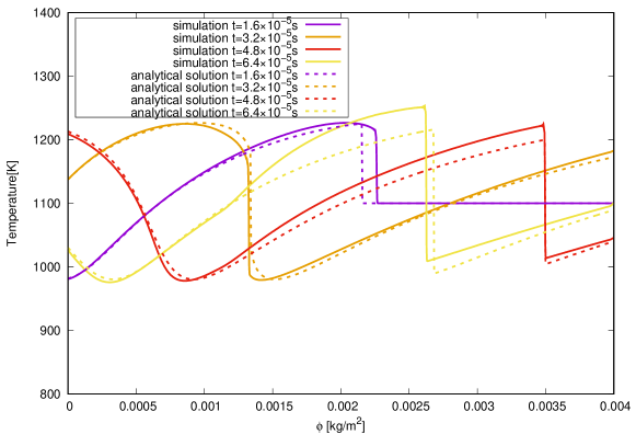
Figure 10: Temperature profiles at select times corresponding to the profiles of Fig. 9.

4.4 Corrections for shock dissipation

The analytical model described above neglects the energy dissipation of internal shocks. Our ignition simulations described below show that the cumulative effect of many internal shocks can have a non-negligible effect on ignition, particularly for cases of very high frequency forcing, where an igniting particle undergoes repeated shocking before it ignites. It is thus of interest to correct the model above and incorporate the energy dissipation of internal shocks. To this effect, a simple correction scheme is to use the shock strength obtained in the model above, and estimate the irreversible temperature increase via the exact shock jump equations. The shock strength is evaluated from the jump in particle speed across each shock. Figure 11 left shows the resolved inner shock Mach number along the Lagrangian space for each inner shock. Figure 11 right evaluates the additional temperature increase for each inner shock. This additional temperature increment is evaluated by shocking the gas in front of the inner shock and then expanding it isentropically to the pre-shocked pressure.

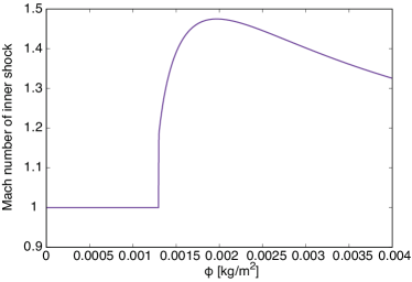
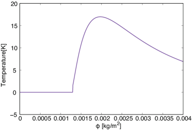
Figure 11: Evolution of the Mach number of the internal shock wave (left) and the corresponding irreversible increase across the shock (right).

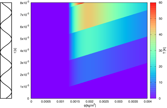
Figure 12: The irreversible temperature gain map due to inner shock waves in $2H_{2}$+$O_{2}$ mixture at state 1 with $A=325$ m/s.

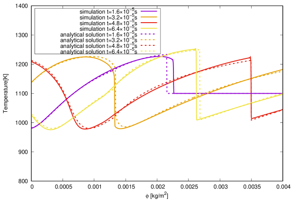
Figure 13: Temperature profiles obtained numerically (solid lines) and analytically (broken lines) in $2H_{2}$+$O_{2}$ mixture at state 1 with $A=325$ m/s.

The additional temperature correction is shown in Fig. 12. The dissipation becomes finite once the inner shocks form at approximately $\phi^{*}$=0.00126kg/m² in this case. The increasing of the fluctuation amplitude and the frequency would shorten this distance. To the right of this boundary is the highest region of shock dissipation, which decays as the inner ”N” wave structure decay.

The corrected temperature evolution is shown in Fig. 13. The temperature amplitude is now in excellent agreement with numerics.

4.5 Problem B: Reflected waves on the lead shock

The disturbances generated along the C+ characteristics described above in Problem A finally reflect on the lead shock, generating a wave of opposite nature on the C- characteristics (expansion for an incident compression, and vice-versa) and an temperature (entropy) disturbance on the particle path. At the level of approximation considered, these reflected disturbances propagate along straight lines $d\phi/dt=-\rho_{1}c_{1}$ for the C- characteristics and $d\phi/dt=0$ for the particle paths by definition and the lead shock path is a straight line. Appendix B provides the details of this problem. Note that the reflected acoustic disturbances are much weaker than the entropy waves, hence re-reflections between these waves with other incident waves are not treated.

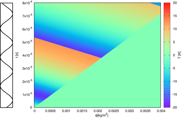
Figure 14: Temperature gain contribution due to C- reflected waves due to the reflection of C+ waves interacting with the lead shock in $2H_{2}$+$O_{2}$.

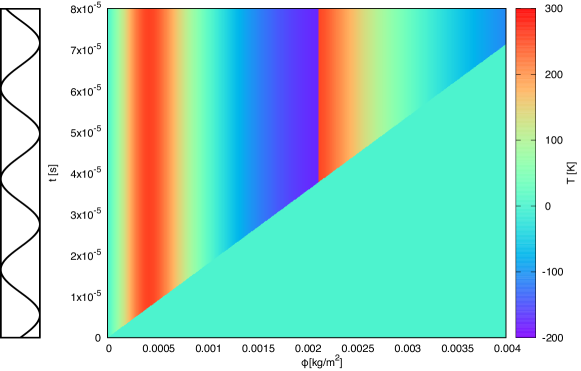
Figure 15: Temperature gain contribution due to entropy waves generated at the lead shock from C+ waves reflected at the lead shock in $2H_{2}$+$O_{2}$.

The entire solution for reflected waves can thus be obtained by the method of characteristics. The temperature perturbations due to the reflected acoustic disturbances are shown in Fig. 14 while the temperature perturbations in Fig. 15 for the chemically frozen $2H_{2}$+$O_{2}$ mixture with post shock temperature of $T_{1}=1100K$ and fluctuation frequency of $f=45.35$kHz.

These two solutions can be linearly combined along with the solution of problem A to obtain the desired solution for temperature evolution in the induction zone. The approximate solution illustrated in Fig. 16 is found in general good agreement with the full numerical solution of Fig. 6. The timing and amplitude of the various events are well-reproduced. Note however that the central part of the hot spots are predicted to be approximately 5$\%$ hotter than the full simulation results; likewise, cooler portions are under-predicted by the approximate model by a similar amount.

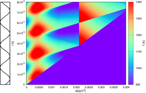
Figure 16: Analytically reconstructed temperature field for $2H_{2}$+$O_{2}$ at conditions of Table 1 and $A=0.2u_{p0}$ and $f=45.4$ kHz without chemical reaction.

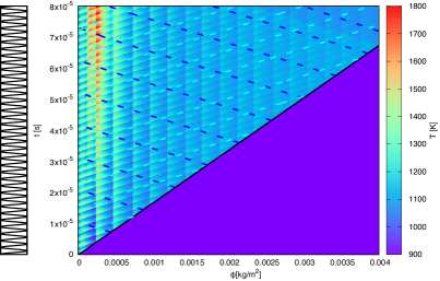
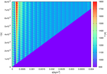
Figure 17: Temperature field obtained numerically (left) and analytically (right) for $2H_{2}$+$O_{2}$ at conditions of Table 1, $A=0.2u_{p0}$ and $f=454$ kHz without chemical reaction.

The gasdynamic model formulated revealed the most important effects to consider in the interpretation of the reactive problem, namely the propensity to form inner shocks at a finite distance from the piston. These inner shocks generate entropy and the cumulative effect may generate the strongest hotspots. Second in order of importance are the reflections of these shocks on the lead shock, generating temperature perturbations by strengthening the lead shock. Note that the inner shocks decay as N-waves as $1/t$. In problems with very high frequency, the resulting temperature increase near the piston dominates the temperature increase away from the piston. An example is shown in Fig. 17 obtained numerically and using the approximate model developed. In this case, the fluctuation frequency is increased to 10 times the value as the case shown in Fig. 6. The strongest hotspot is dominated by the inner shock dissipation. Overall, the analytical results predict very well the location and temperature of the hot spot.

5 The reactive problem solution

5.1 Fuels and their characteristic ignition and reaction times

Shock-induced ignition and transition to detonation was studied in two reactive mixtures spanning the different behaviour of ignition observed in practice, namely $2H_{2}+O_{2}$ and $C_{2}H_{4}+3O_{2}$ at temperatures of approximately 1100K, which is the lower end temperatures permitting sufficiently rapid auto-ignition and transition to detonation in practice. For the $2H_{2}+O_{2}$ mixture, a post-shock temperature of $T_{1}=1100$K and post-shock pressure of $p_{1}=1$atm are obtained by a piston with mean speed 1626 m/s moving into a gas at an initial temperature of $T_{0}=300$K and initial pressure of $p_{0}=6$kPa. This choice was also motivated by the abundance of experiments on reference ignition data, e.g., induction delay, for hydrogen-oxygen at 1 atm, as well as addressing the final stages of DDT where sufficiently strong shocks are generated in this range of temperatures. Moreover, approximately 1100 K is the lower limit of high-temperature ignition for hydrogen-oxygen ignition at 1 atm (Meyer & Oppenheim, 1971). The test conditions for $C_{2}H_{4}+3O_{2}$ were $T_{0}=300$K and $p_{0}=6.2$ kPa, with a mean piston of $u_{p0}=1259$m/s, which brings the post shock conditions to those studied by Saif (2016) in deflagration to detonation transition experiments. Table 1 lists the relevant mixture properties at these conditions. We first characterized the relevant time scales in the two mixtures in constant volume calculations; the piston forcing characteristics will be referenced to the relevant chemical times. We define the ignition delay time $t_{i}$ at constant volume as the time elapsed until maximum thermicity. For a mixture of ideal gases, the thermicity reduces to (Fickett & Davis, 1979; Williams, 1985; Kao & Shepherd, 2008):

$$\dot{\sigma}=\sum\limits_{i=1}^{N}\left(\frac{\bar{W}}{W_{i}}-\frac{h_{i}}{c_{p}T}\right)\frac{DY_{i}}{Dt}$$ (25)

where $W_{i}$ is the molecular weight of the i${}^{\text{th}}$ component, $\bar{W}$ is the mean molecular weight of the mixture, $h_{i}$ is the specific enthalpy of the i${}^{\text{th}}$ specie and $c_{p}$ is the mixture frozen specific heat and $Y_{i}$ is the mass fraction of the i${}^{\text{th}}$ specie in the mixture of $N$ total number of species. The other relevant chemical time is the exothermic reaction time $t_{r}$, during which energy release affects the dynamics of the gas. It is defined as the inverse of the maximum thermicity. These two time scales are reported in Table 1. The ethylene mixture is characterized by a much larger ratio of these two time scales $\Lambda=t_{i}/t_{r}$. This value lies at the lower range of most hydrocarbons, which partly motivates our selection of this mixture. Very large values are computationally prohibitive, since the reaction time and length scales require sufficient resolution. Figure 18 shows the evolution of temperature and thermicity for the two fuels.

Table 1: Relevant thermo-chemical properties of the two reacting mixtures.

	$T_{0}$	$P_{0}$	$u_{p0}$	$T_{1}$	$P_{1}$	$\rho_{1}c_{1}$	$T_{a}/T_{1}$	$t_{i0}$	$t_{r}$
	(K)	(Pa)	(m/s)	(K)	(Pa)	(kg/m2/s)		(s)	(s)
2H2+O2	300	$5.90\times 10^{3}$	$1.63\times 10^{3}$	1100	$1.01\times 10^{5}$	136.2	8.7	$3.3\times 10^{-5}$	$2.0\times 10^{-6}$
C2H4+3O2	300	$6.2\times 10^{3}$	$1.26\times 10^{3}$	1069	$1.46\times 10^{5}$	298.7	22	$1.4\times 10^{-3}$	$1.0\times 10^{-6}$

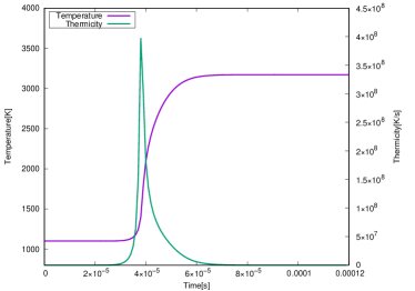
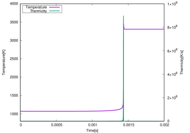
Figure 18: Temperature and thermicity evolution at constant volume for $2H_{2}+O_{2}$ (left) and $C_{2}H_{4}+3O_{2}$ (right) taking state 1 (see Table 1) as initial condition.

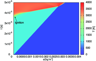
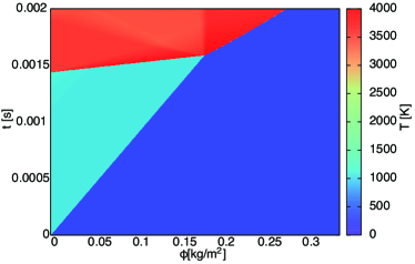
Figure 19: Shock induced ignition in $2H_{2}+O_{2}$ (left) and $C_{2}H_{4}+3O_{2}$ (right) without perturbations; the initial conditions in the pre-shock region are zero velocity and state 0, with piston velocities given in Table 1; the post shock state is state 1.

5.2 Ignition and transition to detonation without fluctuations

The dynamics of shock induced ignition were first studied in the absence of fluctuations. Figure 19 shows the evolution of the temperature field. For the hydrogen mixture, the first ignition along the piston path occurs approximately at the constant volume ignition time, since prior to this event, the lack of thermal evolution keeps the gas shocked by the lead shock at the constant post shock state. The subsequent rapid acceleration of the reaction zone and formation of an internal shock on the time scale of energy deposition $t_{r}$ is characteristic of such dynamics; these internal dynamics are compatible with the model of Sharpe (2002). The rapid internal acceleration of the fast flame leads to the development of an internal Chapman-Jouguet detonation wave, followed by a Taylor wave (Yang et al., 2023). The arrival of the internal detonation wave at the lead shock transmits an overdriven detonation wave in the quiescent gas, which eventually decays towards the CJ condition as the expansion wave trailing it penetrates the wave structure. The transition sequence for the ethylene mixture follows a similar sequence, but the rapid initial transition occurs faster, on time scales of $t_{r}$, which are much shorter than the ignition delay time scale in this case.

5.3 Slow forcing

When the forcing period is longer than the induction delay, the sequence of events leading to auto-ignition resemble qualitatively the ignition sequence without fluctuations. An example is shown in Fig. 20 for the hydrogen system. The slow compression of the gas in the induction zone shortens the ignition delay $2.5\times 10^{-5}s$. One could modify the analysis of Sharpe (2002) to account for the non-uniform conditions in a straightforward, albeit algebraically complex manner. Note the the phase of the fluctuation is important here. Initial cooling of the induction zone gas would have the opposite effect to delay the ignition.

When the period of the fluctuation becomes comparable with the induction delay, it modifies the induction time gradient more significantly and can give rise to first ignition away from the piston face. An example is shown in Fig. 21 for the ethylene mixture. The gradient of ignition delay set up by the lead shock and modulated by the piston non-steadiness can be flatter. Its phase velocity approaches the speed of acoustic signals $\pm\rho_{1}c_{1}$, leading to more prompt acceleration by the Zel’dovich gradient mechanism (Sharpe & Short, 2003) in both directions.

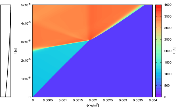
Figure 20: Shock induced ignition with $2H_{2}+O_{2}$, $f=4.535kHz$, $A=20\%u_{p}$

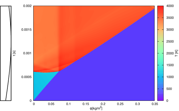
Figure 21: Shock induced ignition in $C_{2}H_{4}+3O_{2}$ with $f=0.2kHz$, $A=0.2u_{p0}$.

5.4 Forcing on induction time scales

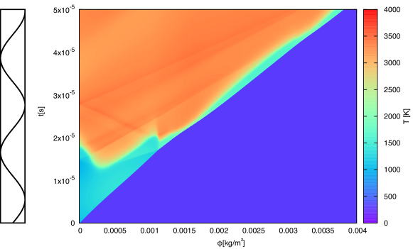
Figure 22: Shock induced ignition in $2H_{2}+O_{2}$ with $f=45.4$ kHz and $A=0.2u_{p0}$.

When the forcing frequency is further increased, the non-linearity results in stronger lead shocks by the inert mechanism discussed above, but the phase velocity of the fast flames are now larger than the acoustic speeds, resulting in de-coherence of the Zel’dovich mechanism. Figure 22 shows a striking example of this situation. The first ignition begins at $t=1.3\times 10^{-5}s$. The spontaneous wave from the first ignition generates a forward and backward shock, which are out of phase with the fast flame. The forward facing shock catches up to the lead shock and generates the second hotspot at $\phi=1.2\times 10^{-3}kg/m^{2}$. The fast flame evolving from the second hotspot is now in phase with the acoustics, resulting in detonation formation. After this 1D detonation structure forming, the reaction zone length oscillates almost in phase with the fluctuation, but the reaction never decouples from the lead shock. Some weak shocks can be observed in the reacted gas with some complex forward and backward patterns. They are formed by interaction between the previous inner shock and the boundary (piston or lead shock wave). Since these shock waves are not in the reaction zone, they do not influence the detonation formation process.

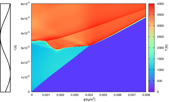
Figure 23: Shock induced ignition in $C_{2}H_{4}+3O_{2}$ with $f=20$ kHz and $A=0.2u_{p0}$.

A similar hotspot ignition mechanism was also observed in the ethylene-oxygen system. The first ignition starts on the first hotspot at $t=2.80\times 10^{-5}s$. Different from the hydrogen-oxygen ignition, the spontaneous wave generates two stronger shock waves and the forward propagating shock wave keeps in phase with the reaction front until it reaches the lead shock. The detonation forms prior to the reaction zone reaching the second hotspot. The backward propagating shock wave decouples from the reaction front and reflects on the piston prior to the reaction front.

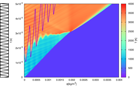
Figure 24: Shock induced ignition in $2H_{2}+O_{2}$ with $f=454$ kHz and $A=0.2u_{p0}$; purple line denotes the ignition locus prediction without coupling to the gas exothermicity predicted by coupling of (26) and the analytical temperature field of section 4.

5.5 Forcing periods between $t_{i}$ and $t_{r}$

When the forcing frequency is increased such that the nominal induction zone counts many forcing periods, a sequence of hot spots are observed. Figure 24 shows this interesting regime for the hydrogen-oxygen case for a frequency of $453.5kHz$ and amplitude $A=0.2U_{p0}$. The higher frequency no longer significantly shortens the delay to first ignition at hot spots, since the inner shock amplitudes remains controlled by the fluctuation amplitude, which is kept constant. The slight reduction in ignition delay in this case is due to the residual repeated shock energy dissipation modelled in the previous section. Instead, a series of sub-critical hotspots are generated along particle paths where internal shocks locally amplified the lead shock. These hotspots can be clearly identified as vertical particle paths originating from the confluence of internal shocks with the lead shock. Note that the higher frequency modulates the trajectory of the fast flame. The saw-tooth fast flame trajectories are now significantly out of phase with the acoustics. This phenomenon is particularly striking in the more sensitive ethylene system illustrated in Fig. 25. Owing to the much larger effective activation energy of the induction kinetics, the hotspots are igniting much earlier than cold spots and the sawtooth fast flames are even more out of phase with the acoustics.

To help us in the interpretation of the mechanism of ignition, we made use of the temperature field prior to ignition determined in section 4, in order to determine the locus of the fast flame without account of exothermicity. For this purpose, the induction layer is modelled in a conventional way by

$$\frac{\partial\zeta}{\partial t}|_{\phi}=k\exp\left(-\frac{T_{a}}{T}\right)$$ (26)

where $\zeta$ is the induction progress variable ranging from 0 (fresh gases) to 1 (end of induction time) and the constants $k$ and $T_{a}$ are calibrated to recover the correct ignition delay and sensitivity to temperature. These are calibrated for constant volume calculations in Cantera. They yield $T_{a}=9562.2$K and $k=1.6118\times 10^{8}s^{-1}$ for the hydrogen-oxygen mixture and $T_{a}=23825.0$K and $k=3.452\times 10^{12}s^{-1}$ for the ethylene mixture at these operating conditions. Given the temperature field, integration of (26) yields the ignition delay $t_{i}(\phi)$ along a particle path implicitly:

$$1=\int_{t_{S}}^{t_{i}}k\exp\left(-\frac{T_{a}}{T(t)}\right)\mathrm{dt}$$ (27)

where $t_{S}(\phi)$ is the lead shock time.

Figure 24 shows how the sequence of hotspots are formed and compares their location with the zero-order prediction. While each sequential hotspot is formed from the coalescence of the internal shock with the lead shock, we note that the ignition delay of each hotspot is successively shorter than the previous one. This is very well predicted by the ignition model with no exothermicity coupling. The mechanism of this reduction is the cumulative energy dissipation heating along a particle path. Nevertheless, we observe that by the 4th hotspot, the energy release from previous hotspots has now played a sensible role in shortening the induction time. This is due to the strengthening of forward facing shock waves passing through the main reaction zone. The sequence of forward facing shocks are thus amplified by energy release. After the 6th hotspot, the sequence of hotspots become in phase with the motion of one of the inner shocks. We thus see a discrete like gradient amplification mechanism with in phase sequence of hotspots with acoustics. This is an example of the type of discrete SWACER mechanism operating. We label these hotspot cascades.

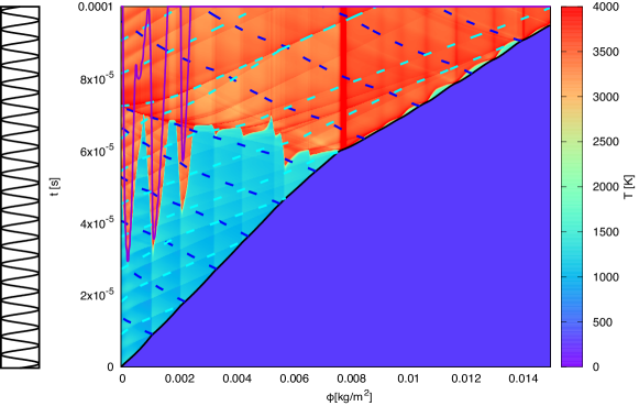
Figure 25: Shock induced ignition in $C_{2}H_{4}+3O_{2}$ with $f=200$ kHz and $A=0.2u_{p0}$; purple line denotes the ignition locus prediction without coupling to the gas exothermicity predicted by coupling of (26) and the analytical temperature field of section 4.

More complex hotspot cascades can be observed in more sensitive mixture. Figure 25 shows the ethylene-oxygen ignition with fluctuation frequency in $200kHz$ and amplitude in 20% of the mean speed. The first ignition starts at $t=2.2\times 10^{-5}s$ form the first hotspot - this is very well predicted by the uncoupled ignition model. Nine hotspot ignitions can be observed prior to the reaction front merging to the lead shock and detonation formation. The second hot-spot is also very well predicted by the model. The third, however, is accelerated by the energy release of the previous two, transmitted along the forward shocks originating from the first two. The three first hotspots thus follow the hotspot cascade mechanism described above.

Nevertheless, the arrival of the first shock amplified by the hotspot cascade at the lead shock creates a strong enough disturbance to lead to prompt ignition at the hotspot along $\phi=0.006$ (hotspot 7). This localized energy release triggers the backwards sequence of promoting the ignition of hotspot 6 and 5 and 4. It also triggers the sequence of hotspots 8 and 9, aided by the shock from hotspot 3. Note that the internal transitions follow again a discrete version of the gradient or SWACER mechanism. We refer to this more complex situation as ”bifurcated hot-spot cascade”, since forward and backward hotspot avalanches are present due to hotspot - lead shock feedback.

5.6 Fast forcing

Once the ignition delay is much longer than the fluctuation period, the hotspot cascade mechanism disappears. Figure 26 shows the pattern for hydrogen-oxygen ignition with frequency in $4535kHz$ and amplitude of 20% of the mean speed. The first ignition starts near the piston at $t=1.0\times 10^{-5}s$. The ignition delay gradient of the first hot spot is very large, since this is controlled by the frequency of forcing, as explained above. Furthermore, the very rapid decay of the N-waves driven by the piston means that irreversible internal dissipation heating by internal shock waves is restricted to the first few generations of hotspots. This further exacerbates the gradient of the first fast flame. As a result, we approach a regime of single hotspot ignition, followed by a region of very weak fluctuations. Although the first ignition delay is very short, the detonation front forms relatively late. Compared to the non-fluctuation case (Fig. 19), the inner supersonic reaction front forms almost at the same time. The place and time of merging between the inner supersonic reaction front and the lead shock does not have significant changes. This very high frequency fluctuation does not make a significant contribution to reducing the time of the detonation formation in this 1D ignition problem.

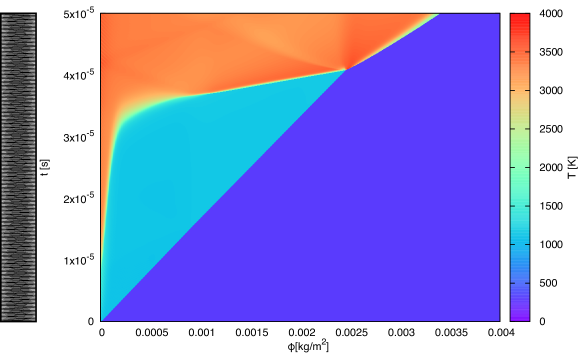
Figure 26: Shock induced ignition in $2H_{2}+O_{2}$ with $f=4540$ kHz and $A=0.2u_{p0}$.

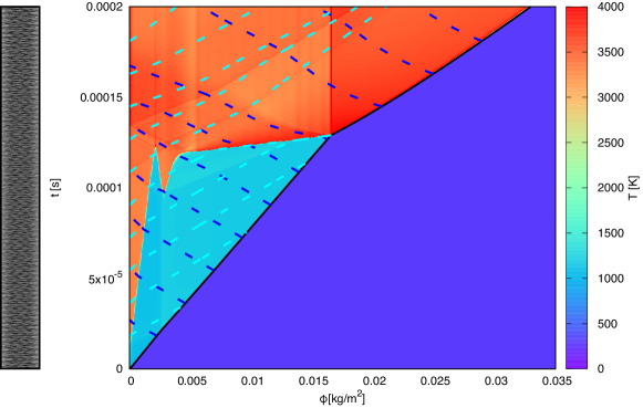
Figure 27: Shock induced ignition in $C_{2}H_{4}+3O_{2}$ with $f=2000$ kHz and $A=0.2u_{p0}$.

A similar pattern was observed for the more sensitive ethylene-oxygen system. Figure 27 shows the ignition diagram with fluctuation frequency in $2000kHz$ and amplitude in 20% of the mean speed. In this case, the ignition delay has been shortened at $t=1.3\times 10^{-5}s$ but the supersonic reaction wave takes longer to form. Two hotspots are formed in this case. The first hotspot is generated from the dissipation. The second hotspot formed by the complex hotspot cascade mechanism which is the interaction between the lead shock and intensified inner shock. In this mixture, the ignition delay is much more sensitive than the hydrogen-oxygen mixture. The intensified shock wave is strong enough to generate an ignition hotspot. This hotspot ignition locus quickly accelerate to an inner detonation, which catches up to the main shock. These inner dynamics shorten the formation distance of the final detonation by approximately 90% as compared to the nominal non-fluctuated case and cannot be neglected.

6 Further discussion

The effect of the forcing frequency and forcing amplitude on the ignition delay of the first spot is shown in Fig. 28 for the two mixtures studied for 16 hydrogen-oxygen cases and 16 ethylene-oxygen cases. All the cases have been categorized into four groups by their forcing strength which ranges from 0.05$u_{p0}$ to 0.2$u_{p0}$. The ignition delay has been normalized by the original ignition delay without forcing: $t_{i0}$. The frequencies have been normalized by $f_{i}=1/t_{i0}$. These results were obtained numerically by solving the full Lagrangian problem. These are well predicted by the ignition model without coupling, as discussed above. The effect of the forcing amplitude is to reduce the ignition delay, as it provides stronger hotspots, as expected. The effect of the forcing frequency is however more interesting and reveals the role of the energy dissipation by shock heating. It also shows that increasing frequency reduces the ignition delay time. With increasing frequency, a particle of gas experiences more heating from the higher number of repeated shock interactions. The ignition delay is thus decreased by the increase in the total energy dissipation. Note also that the ignition delay reduction is much more substantial in the ethylene system, owing to the stronger sensitivity of ignition kinetics to temperature.

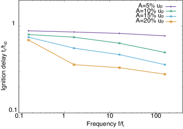
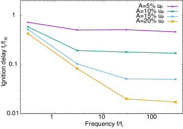
Figure 28: Ignition delay of the first hot spot for $2H_{2}+O_{2}$ (left) and $C_{2}H_{4}+3O_{2}$ (right) for different perturbation frequency and amplitude.

The mechanisms of pressure wave enhancement identified in the present paper is in agreement with the gradient mechanism of Zel’dovich or the SWACER mechanism. The physics operating in the low frequency regime is in line with the runaway mechanism for arbitrary gradients studied in the past by Sharpe & Short (2003). Changes in the forcing frequency changes the lead shock strength distribution, hence the induction delay distribution. With increasing frequency, the fast flame from each distinct spot becomes less in phase with the acoustics. The run-away process now relies on the sequence of hotspots being in phase with acoustics. Two cascade mechanisms were identified. The first relies on the energy release of a previous hot-spot to strengthen a forward facing compression wave. This in turn shortens the ignition delay of the next hot spot, and so-forth. This mechanism is the discrete version of shock to detonation transition modelled by Sharpe (2002).

The second cascade mechanism occurs in sufficiently sensitive systems (high activation energy). The first generation cascade amplifies a shock that arrives at the lead shock prior to the cascade culminating in transition to detonation. The shock-shock interaction triggers a second generation of hotspots cascades of the first type.

Interestingly, these hotspot cascades permit for detonations to form on the same time scales as the shortest ignition delay. Figure 29 shows the detonation formation time for all the cases studied. These time scales are comparable with those of Fig. 28. The gasdynamic model developed is thus sufficient to determine this time of first ignition. It is only for sufficiently high frequency oscillations that the cascades are suppressed by the mechanism of inner N-wave decay, reducing the effective penetration distance of the energy dissipation, as discussed above. The inner shock decay results in a more pronounced gradient in hot-spot ignition gradient, suppressing the coherence between hot-spots and shocks. At these high frequencies, the time to detonation actually increases with increasing frequency. In the limit of high frequency, only one generation of hotspots near the piston remains, leading to prompt first ignition but unfavourable gradient.

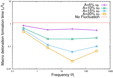
Figure 29: Detonation formation time for $2H_{2}+O_{2}$ (left) and $C_{2}H_{4}+3O_{2}$ (right) for different perturbation frequency and amplitude.

While the problem studied is a very canonical one, it may find direct application in the understanding of the late phases of deflagration to detonation transition, where transonic turbulent flames are generated (Saif et al., 2017; Poludnenko et al., 2019). A highly non-steady turbulent flame generating high frequency mechanical oscillations may trigger such hot-spot cascades. When they are transonic, parts of their energy release is in phase with the acoustics. Likewise, unstable detonations rely on high frequency oscillations to intermittently re-amplify and survive quenching (Radulescu & Sow, 2023; Sow et al., 2023). The role of gasdynamic coupling with hot-spots is at the heart of these problems.

7 Conclusion

Our study of ignition behind a shock driven by an oscillating piston has revealed the intricate role of mechanical fluctuations on the ignition process and run-away to detonation. A substantial decrease in the ignition delay was observed, owing to the changes in the lead shock strength. With increasing frequency of oscillation, the role of lead shock modulation was decreased in favour of the role of the internal shock wave motion and resulting dissipative heating. The internal shock wave motion permitted hotspot cascades, the organization of sequential hot spots in phase with the acoustics. However, further increase in forcing frequency suppressed the cascade mechanism.

The present paper shows conclusively that the high frequency forcing can play a very substantial role in the transition from a shock-induced ignition to detonation. The results may thus clarify the general experimental observations of anomalous ignition in deflagration to detonation transition in turbulent flames and analogous phenomena within very unstable detonation waves.

Declaration of Interests

The authors report no conflict of interest.

Appendix A Transformation of the Euler equations for a multi-component reactive gas to Lagrangian coordinates

We derive the Lagrangian form of the governing equations for a multi-component reactive medium and their characteristic form, generalizing the results obtained by Fickett et al. (1970) for a single irreversible reaction.

A.1 The reactive Euler equations in lab-coordinates

The reactive Euler equations are well known in Eulerian, or lab coordinates. In 1D, they can be written as:

$$\frac{D\rho}{Dt}+\rho\frac{\partial u}{\partial x}=0$$ (28)

$$\rho\frac{Du}{Dt}+\frac{\partial p}{\partial x}=0$$ (29)

$$\rho\frac{De_{tot}}{Dt}+\frac{\partial(pu)}{\partial x}=0$$ (30)

$$\rho\frac{DY_{i}}{Dt}=\omega_{i}$$ (31)

where $e_{tot}=e+\frac{1}{2}u^{2}$ is the total energy, $e$ the specific internal energy of the mixture, $Y_{i}$ the mass fraction of the i${}^{\text{th}}$ component and $\omega_{i}$ the mass production rate of specie $i$ per unit volume, per unit time, obtained from chemical kinetics. After some thermodynamic manipulations, the energy equation (30) can be also written as

$$\frac{Dp}{Dt}=c^{2}\frac{D\rho}{Dt}+\rho c^{2}\dot{\sigma}\\$$ (32)

where $\dot{\sigma}$ is the thermicity, which denotes the gasdynamic effect of chemical reactions or other relaxation phenomena on the rate of pressure and speed changes along the family of characteristics. The thermicity in its most general form is given by:

$$\dot{\sigma}=-\frac{\rho}{c_{p}}\left(\frac{\partial v}{\partial T}\right)_{p,Y_{i}}\sum_{i=1}^{N}\left(\frac{\partial h}{\partial Y_{i}}\right)_{p,\rho,Y_{j,j\neq i}}\frac{DY_{i}}{Dt}$$ (33)

(Fickett & Davis, 1979). For a mixture of ideal gases, the thermicity reduces to

$$\dot{\sigma}=\sum\limits_{i=1}^{N}\left(\frac{\bar{W}}{W_{i}}-\frac{h_{i}}{c_{p}T}\right)\frac{DY_{i}}{Dt}$$ (34)

where $W_{i}$ is the molecular weight of the i${}^{\text{th}}$ component, $\bar{W}$ is the mean molecular weight of the mixture, $h_{i}$ is the specific enthalpy of the i${}^{\text{th}}$ specie and $c_{p}$ is the mixture frozen specific heat.

The characteristic equations are obtained by simple manipulations of these expressions and yield

$$\frac{D_{\pm}p}{Dt}\pm\rho c\frac{D_{\pm}u}{Dt}=\rho c^{2}\dot{\sigma}\\$$ (35)

where

$$\frac{D_{\pm}}{Dt}\equiv\frac{\partial}{\partial t}+(u\pm c)\frac{\partial}{\partial x}$$ (36)

are derivatives along the C+ and C- characteristics, given respectively by $dx/dt=u\pm c$.

A.2 Lagrangian coordinates and transformation rules

In 1D problems where one boundary condition can be prescribed along a particle path $x_{p}(t)$, where $u=\dot{x}_{p}(t)$, $\rho=\rho_{p}(t)$, etc., we can change from an Eulerian frame to a Lagrangian frame, by transforming the reactive Euler equations expressed with independent variables $(x,t)$ to Lagrangian independent variables $(\phi,t^{\prime})$ by the formal change of variables:

$$\phi=\int_{x_{p}(t)}^{x}\rho\mathrm{d}x,\qquad t^{\prime}=t$$ (37)

The density weighted coordinate $\phi$ remains constant along a particle path through the conservation of mass, as we will show below. Equations (37) permit to evaluate the derivatives $\left(\partial\phi/\partial x\right)_{t}$ and $\left(\partial\phi/\partial t\right)_{x}$ required for the change of variables. Using the Leibniz rule of differentiation of an integral where both the integrand and the integral bounds vary with the variable used for differentiation, we obtain:

$$\left(\frac{\partial\phi}{\partial x}\right)_{t}=\rho,\qquad\left(\frac{\partial\phi}{\partial t}\right)_{x}=\int_{x_{p}(t)}^{x}\frac{\partial\rho}{\partial t}\mathrm{d}x-\rho_{p}\dot{x}_{p}$$ (38)

To evaluate the last integral in (38), we make use of the continuity equation (28) re-written as,

$$\frac{\partial\rho}{\partial t}+\frac{\partial\rho u}{\partial x}=0$$ (39)

and obtain

$$\left(\frac{\partial\phi}{\partial x}\right)_{t}=\rho,\qquad\left(\frac{\partial\phi}{\partial t}\right)_{x}=-\rho u$$ (40)

Using (40), it can be verified that the variation of $\phi$ along a particle path, namely,

$$\frac{D\phi}{Dt}\equiv\left(\frac{\partial\phi}{\partial t}\right)_{x}+u\left(\frac{\partial\phi}{\partial x}\right)_{t}=0$$ (41)

is indeed zero and $\phi$ serves as a particle label.

We can now operate the formal change of variables using (40) and the chain rule of differentiation for any field variable $a\left(\phi(x,t),t^{\prime}(x,t)\right)$, yielding the following:

$$\left(\frac{\partial a}{\partial x}\right)_{t}=\left(\frac{\partial a}{\partial\phi}\right)_{t^{\prime}}\left(\frac{\partial\phi}{\partial x}\right)_{t}+\left(\frac{\partial a}{\partial t^{\prime}}\right)_{\phi}\left(\frac{\partial t^{\prime}}{\partial x}\right)_{t}=\rho\left(\frac{\partial a}{\partial\phi}\right)_{t^{\prime}}$$ (42)

$$\left(\frac{\partial a}{\partial t}\right)_{x}=\left(\frac{\partial a}{\partial\phi}\right)_{t^{\prime}}\left(\frac{\partial\phi}{\partial t}\right)_{x}+\left(\frac{\partial a}{\partial t^{\prime}}\right)_{\phi}\left(\frac{\partial t^{\prime}}{\partial t}\right)_{x}=-\rho u\left(\frac{\partial a}{\partial\phi}\right)_{t^{\prime}}+\left(\frac{\partial a}{\partial t^{\prime}}\right)_{\phi}$$ (43)

The above two expressions can also be used for substitution expressions for derivatives along particle paths:

$$\frac{Da}{Dt}\equiv\left(\frac{\partial a}{\partial t}\right)_{x}+u\left(\frac{\partial a}{\partial x}\right)_{t}=\left(\frac{\partial a}{\partial t^{\prime}}\right)_{\phi}$$ (44)

and along C+ and C- characteristics:

$$\frac{D_{\pm}a}{Dt}\equiv\left(\frac{\partial a}{\partial t}\right)_{x}+(u\pm c)\left(\frac{\partial a}{\partial x}\right)_{t}=\left(\frac{\partial a}{\partial t^{\prime}}\right)_{\phi}\pm\rho c\left(\frac{\partial a}{\partial\phi}\right)_{t^{\prime}}$$ (45)

A.3 The reactive Euler equations in Lagrangian coordinates

Equations (42) to (45) now permit to re-write the reactive Euler equations (28)-(31) as:

$$\frac{\partial v}{\partial t^{\prime}}-\frac{\partial u}{\partial\phi}=0$$ (46)

$$\frac{\partial u}{\partial t^{\prime}}+\frac{\partial p}{\partial\phi}=0$$ (47)

$$\frac{\partial e_{tot}}{\partial t^{\prime}}+\frac{\partial pu}{\partial\phi}=0$$ (48)

$$\frac{\partial Y_{i}}{\partial t^{\prime}}=\frac{\omega_{i}}{\rho}$$ (49)

where $v=1/\rho$ is the specific volume.

The alternate form of the energy equation (32) becomes

$$\frac{\partial p}{\partial t^{\prime}}=c^{2}\frac{\partial p}{\partial t^{\prime}}+\rho c^{2}\dot{\sigma}\\$$ (50)

and the characteristic equation (35) becomes

$$\left(\frac{\partial}{\partial t^{\prime}}\pm\rho c\frac{\partial}{\partial\phi}\right)p\pm\rho c\left(\frac{\partial}{\partial t^{\prime}}\pm\rho c\frac{\partial}{\partial\phi}\right)u=\rho c^{2}\dot{\sigma}\\$$ (51)

We remark that the C+ and C- characteristics are given by

$$\frac{\mathrm{d}\phi}{\mathrm{d}t^{\prime}}=\pm\rho c$$ (52)

and the characteristic speeds are $\pm\rho c$.

Appendix B Reflected disturbances at the lead shock

We consider the problem of a weak disturbance propagating along a C+ characteristic overtaking a lead shock of arbitrary strength, generating a reflected acoustic disturbance along a C- characteristic and a entropy wave along a particle path. Fig. 31 illustrates the various states: State 1 is the post shock state, state 2 is the post incident disturbance state, state 4 is the state behind the reflected acoustic disturbance and state 3 is the state behind the modified lead shock. The upstream uniform state 0 and states 1 and 2 are known and we seek to determine states 3 and 4. The original incident shock has Mach number $M_{i}$, and the new Mach number of the incident shock is disturbance is $M_{t}$. We characterize the inner disturbance by its overpessure, which we take as being a small perturbation $z_{12}=(p_{2}-p_{1})/p_{1}\ll 1$. We thus linearize around state 1, i.e.,

$$p=p_{1}+p^{\prime}$$ (53)

$$\rho=\rho_{1}+\rho^{\prime}$$ (54)

$$T=T_{1}+T^{\prime}$$ (55)

$$M_{t}=M_{0}+M^{\prime}$$ (56)

where the prime quantities are small.

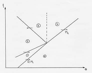
Figure 30: A disturbance catching up to the lead shock, modifying its strength and resulting acoustic and entropy wave generation.

The linearised version of the characteristic equations along the C$\pm$ characteristics becomes:

$$dp^{\prime}\pm\rho_{1}c_{1}du^{\prime}=0$$ (57)

The energy equation for a non-reacting perfect gas along a particle path is

$$\frac{dp}{p}-\frac{\gamma}{\gamma-1}\frac{dT}{T}=0$$ (58)

which linearises to:

$$\frac{p^{\prime}}{p_{1}}-\frac{\gamma}{\gamma-1}\frac{T^{\prime}}{T_{1}}=0$$ (59)

The disturbances in state 3 are related to the change in Mach number via the Rankine-Hugoniot relations:

$$p_{3}^{\prime}=\left(\frac{dp}{dM}\right)_{RH}M^{\prime}$$ (60)

$$u_{3}^{\prime}=\left(\frac{du}{dM}\right)_{RH}M^{\prime}$$ (61)

$$T_{3}^{\prime}=\left(\frac{dT}{dM}\right)_{RH}M^{\prime}$$ (62)

where derivatives with subscript RH are to be taken from the Rankine-Hugoniot relations $p(M)$, $u(M)$ and $T(M)$ respectively. Below, these derivatives are taken with respect to pressure, e.g., $(du/dM)_{RH}=(du/dp)_{RH}(dp/dM)_{RH}$.

Using the method of characteristics, the pressure, speed and temperature disturbances can be found by straightforward solution of the compatibility equations (57) in the acoustic regime considered. Across the incident disturbance, the C- compatibility relation requires

$$p_{1}^{\prime}-\rho_{1}c_{1}u_{1}^{\prime}=0$$ (63)

Across the reflected disturbance, the C+ compatibility relation requires

$$p_{2}^{\prime}-\rho_{1}c_{1}u_{2}^{\prime}=p_{4}^{\prime}-\rho_{1}c_{1}u_{4}^{\prime}$$ (64)

across the contact discontinuity, mechanical equilibrium applies, $u^{\prime}_{3}=u^{\prime}_{4}$ and $p^{\prime}_{3}=p^{\prime}_{4}$. Solving this system of algebraic equations, one obtains the strength of the disturbances in terms of $p_{2}^{\prime}$:

$$u_{2}^{\prime}=\left(\frac{1}{\rho_{1}c_{1}}\right)p_{2}^{\prime}$$ (65)

$$T_{2}^{\prime}=\left(\frac{\gamma-1}{\gamma}\frac{T_{1}}{p_{1}}\right)p_{2}^{\prime}$$ (66)

$$p_{3}^{\prime}=p_{4}^{\prime}=\left(\frac{2}{1+\rho_{1}c_{1}(du/dp)_{RH}}\right)p_{2}^{\prime}$$ (67)

$$u_{3}^{\prime}=u_{4}^{\prime}=\left(\frac{2(du/dp)_{RH}}{1+\rho_{1}c_{1}(du/dp)_{RH}}\right)p_{2}^{\prime}$$ (68)

$$T_{3}^{\prime}=\left(\frac{2(dT/dp)_{RH}}{1+\rho_{1}c_{1}(du/dp)_{RH}}\right)p_{2}^{\prime}$$ (69)

$$T_{4}^{\prime}=\left(\frac{\gamma-1}{\gamma}\frac{T_{1}}{p_{1}}\frac{2}{1+\rho_{1}c_{1}(du/dp)_{RH}}\right)p_{2}^{\prime}$$ (70)

This completes the solution. Figure 31 shows the performance of the acoustic treatment of inner perturbations on the temperatures obtained behind the shock. Comparison is made against exact calculations using the exact jump equations where the inner disturbance is a shock wave and the reflected wave is a centred expansion wave Bull et al. (1954).

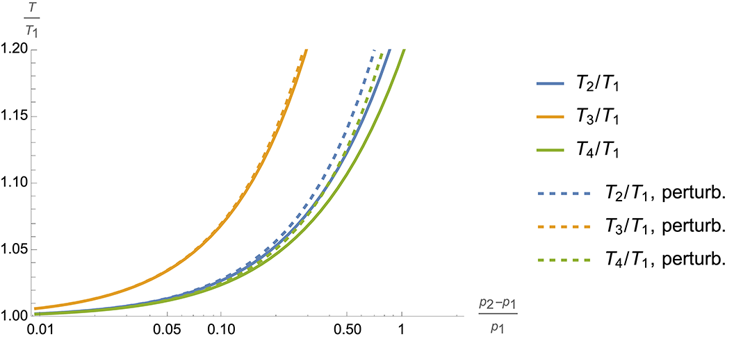
Figure 31: Temperature perturbations behind a $M_{i}=4.05$ lead shock after the catch up of an arbitrary strength shock in a perfect gas with $\gamma=1.348$; full lines is the exact solution while broken lines is the acoustic approximation for the inner disturbance.

Simplifications for weak or strong incident shocks are straightforward. If one assumes a strong lead shock, starting with the usual strong shock RH expressions

$$\frac{u}{D}=\frac{p}{\rho_{0}D^{2}}=\frac{2}{\gamma+1}\quad\textrm{and}\quad\frac{\rho}{\rho_{0}}=\frac{\gamma+1}{\gamma-1}$$ (71)

one obtains

$$p_{3}^{\prime}=p_{4}^{\prime} =\frac{4(\gamma-1)}{2(\gamma-1)+\sqrt{2\gamma(\gamma-1)}}p_{2}^{\prime}$$ (72)

$$u_{3}^{\prime}=u_{4}^{\prime} =\frac{1}{1+\frac{\gamma}{\sqrt{2\gamma(\gamma-1)}}}\frac{p_{2}^{\prime}}{\rho_{0}D}$$ (73)

$$\frac{T_{2}^{\prime}}{T_{1}} =\frac{\gamma-1}{\gamma}\frac{p_{2}^{\prime}}{p_{1}}$$ (74)

$$\frac{T_{3}^{\prime}}{T_{1}} =\frac{4(\gamma-1)}{2(\gamma-1)+\sqrt{2\gamma(\gamma-1)}}\frac{p_{2}^{\prime}}{p_{1}}$$ (75)

$$\frac{T_{4}^{\prime}}{T_{1}} =\frac{4(\gamma-1)^{2}}{\gamma\left(2(\gamma-1)+\sqrt{2\gamma(\gamma-1)}\right)}\frac{p_{2}^{\prime}}{p_{1}}$$ (76)

For weak shocks treated in this paper, the exact Rankine-Hugoniot shock jump conditions can be parametrized by the shock overpressure $z=(p-p_{0})/p_{0}$ and truncated at the desired order. The exact expressions are given by Whitham (1974) :

$$\frac{p}{p_{0}}=1+z,\quad\frac{\rho}{\rho_{0}}=\frac{1+\frac{\gamma+1}{2\gamma}}{1+\frac{\gamma-1}{2\gamma}},\quad\frac{c}{c_{0}}=\sqrt{\frac{p}{p_{0}}\frac{\rho_{0}}{\rho}},\quad\frac{T}{T_{0}}=\left(\frac{c}{c_{0}}\right)^{2}$$

$$\frac{u-u_{0}}{c_{0}}=\frac{z}{\gamma\sqrt{1+\frac{\gamma+1}{2\gamma}}},\quad M=\sqrt{1+\frac{\gamma+1}{2\gamma}}$$ (77)

which permits to re-write the derivatives in terms of $z$, for example

$$\left(\frac{du}{dp}\right)_{RH}=\frac{\left(\frac{du}{dz}\right)_{RH}}{\left(\frac{dp}{dz}\right)_{RH}}=\frac{c_{0}}{p_{0}}\frac{\sqrt{2+z+z/\gamma}\left(z+\gamma(4+z)\right)}{\sqrt{2}\left(z+\gamma(2+z)\right)^{2}}$$ (78)

If one wishes to truncate the approximation to weak incident shocks, while retaining non-linearity, the RH equations can be expanded in Taylor series in terms of $z$ and retain only terms up to $O(z^{2})$, such that entropy and the Riemann variable $J^{-}$ remain constant; the leading contribution to changes in entropy and $J^{-}$ across the shock are terms of order $O(z^{3})$ (Whitham, 1974).

References

- Bull et al. (1954) Bull, G. V., Fowell, L. R. & Henshaw, D. H. 1954 The interaction of two similarly facing shock waves. Journal of the Aeronautical Sciences 21 (3), 210–212, arXiv: https://doi.org/10.2514/8.2968.
- Bychkov et al. (2012) Bychkov, Vitaly, Valiev, Damir, Akkerman, V’yacheslav & Law, Chung K 2012 Gas compression moderates flame acceleration in deflagration-to-detonation transition. Combustion science and technology 184 (7-8), 1066–1079.
- Chandrasekhar (1943) Chandrasekhar, S. 1943 On the decay of planar shock waves. Tech. Rep. 423. Aberdeen Proving Ground.
- Chue et al. (1993) Chue, RS, Clarke, JF & Lee, JH 1993 Chapman-jouguet deflagrations. Proceedings of the Royal Society of London. Series A: Mathematical and Physical Sciences 441 (1913), 607–623.
- Ciccarelli & Dorofeev (2008) Ciccarelli, G & Dorofeev, S 2008 Flame acceleration and transition to detonation in ducts. Progress in energy and combustion science 34 (4), 499–550.
- Dorofeev et al. (2000) Dorofeev, SB, Sidorov, VP, Kuznetsov, MS, Matsukov, ID & Alekseev, VI 2000 Effect of scale on the onset of detonations. Shock Waves 10 (2), 137–149.
- Eder (2001) Eder, Andreas 2001 Brennverhalten schallnaher und überschall-schneller wasserstoff-luft flammen. Dissertation, Technische Universität München, München.
- Eder & Brehm (2001) Eder, A & Brehm, N 2001 Analytical and experimental insights into fast deflagrations, detonations, and the deflagration-to-detonation transition process. Heat and mass transfer 37 (6), 543–548.
- Einfeldt et al. (1991) Einfeldt, Bernd, Munz, Claus-Dieter, Roe, Philip L & Sjögreen, Björn 1991 On godunov-type methods near low densities. Journal of computational physics 92 (2), 273–295.
- Fickett & Davis (1979) Fickett, W. & Davis, W. C. 1979 Detonation theory and experiment. Dover Publication Inc.
- Fickett et al. (1970) Fickett, W., Jacobson, J. D. & Wood, W.W. 1970 The method of characteristics for one-dimensional flow with chemical reactions. Tech. Rep. LA-4269. Los Alamos Scientific Laboratory, Los Alamos, New Mexico, written August 1969.
- Goodwin & Moffat (2017) Goodwin, Moffat HK & Moffat, HK 2017 Dg and rl speth. cantera: an object-oriented software toolkit for chemical kinetics, thermodynamics, and transport processes.
- Kao & Shepherd (2008) Kao, S. & Shepherd, J.E. 2008 Numerical solution methods for control volume explosions and ZND detonation structure. Tech. Rep. GALCIT Report FM2006.007. California Institute of Technology, Pasadena, California.
- Kee et al. (2005) Kee, Robert J, Coltrin, Michael E & Glarborg, Peter 2005 Chemically reacting flow: theory and practice. John Wiley & Sons.
- Lee & Moen (1980) Lee, J.H.S. & Moen, I.O. 1980 The mechanism of transition from deflagration to detonation in vapor cloud explosions. Progress in Energy and Combustion Science 6 (4), 359–389.
- LeVeque et al. (2002) LeVeque, Randall J & others 2002 Finite volume methods for hyperbolic problems, , vol. 31. Cambridge university press.
- Li et al. (2004) Li, Juan, Zhao, Zhenwei, Kazakov, Andrei & Dryer, Frederick L 2004 An updated comprehensive kinetic model of hydrogen combustion. International journal of chemical kinetics 36 (10), 566–575.
- Meyer & Oppenheim (1971) Meyer, J.W. & Oppenheim, A.K. 1971 On the shock-induced ignition of explosive gases. In Symposium (International) on Combustion, , vol. 13, pp. 1153–1164. Elsevier.
- Meyer et al. (1970) Meyer, J.W., Urtiew, P.A. & Oppenheim, A.K. 1970 On the inadequacy of gasdynamic processes for triggering the transition to detonation. Combustion and Flame 14 (1), 13–20.
- Middha & Hansen (2008) Middha, Prankul & Hansen, Olav R 2008 Predicting deflagration to detonation transition in hydrogen explosions. Process Safety Progress 27 (3), 192–204.
- Munz (1994) Munz, CD 1994 On godunov-type schemes for lagrangian gas dynamics. SIAM Journal on Numerical Analysis 31 (1), 17–42.
- Oran et al. (2020) Oran, Elaine S, Chamberlain, Geoffrey & Pekalski, Andrzej 2020 Mechanisms and occurrence of detonations in vapor cloud explosions. Progress in Energy and Combustion Science 77, 100804.
- Oran & Gamezo (2007) Oran, Elaine S & Gamezo, Vadim N 2007 Origins of the deflagration-to-detonation transition in gas-phase combustion. Combustion and Flame 148 (1-2), 4–47.
- Poludnenko et al. (2019) Poludnenko, Alexei Y, Chambers, Jessica, Ahmed, Kareem, Gamezo, Vadim N & Taylor, Brian D 2019 A unified mechanism for unconfined deflagration-to-detonation transition in terrestrial chemical systems and type ia supernovae. Science 366 (6465).
- Radulescu & Sow (2023) Radulescu, Matei & Sow, Aliou 2023 Evidence for self-organized criticality (soc) in the non-linear dynamics of detonations. In Proceedings of the 29th International Colloquium on Dynamics of Explosions and Reactive Systems. SNU Siheung, South Korea, paper 266.
- Rakotoarison et al. (2024) Rakotoarison, Willstrong, Vilende, Yohan, Pekalski, Andrzej & Radulescu, Matei I. 2024 Model for chapman-jouguet deflagrations in open ended tubes with varying vent ratios. Combustion and Flame 260, 113212.
- Rakotoarison et al. (2019) Rakotoarison, W., Vilende, Yohan & Radulescu, M.I. 2019 Model for Chapman-Jouguet deflagrations in open ended tubes with varying vent ratios. In Proceedings of the 27th International Colloquium on Dynamics of Explosions and Reactive Systems. Beijing, China, paper 186.
- Saif (2016) Saif, M. 2016 Run-up distance from deflagration to detonation in fast flames. Master’s thesis, University of Ottawa.
- Saif et al. (2017) Saif, Mohamed, Wang, Wentian, Pekalski, Andrzej, Levin, Marc & Radulescu, Matei I 2017 Chapman–jouguet deflagrations and their transition to detonation. Proceedings of the Combustion Institute 36 (2), 2771–2779.
- Sharpe & Short (2003) Sharpe, G.J. & Short, M. 2003 Detonation ignition from a temperature gradient for a two-step chain-branching kinetics model. Journal of Fluid Mechanics 476, 267–292.
- Sharpe (2002) Sharpe, Gary J. 2002 Shock-induced ignition for a two-step chain-branching kinetics model. Physics of Fluids 14 (12), 4372–4388, arXiv: https://pubs.aip.org/aip/pof/article-pdf/14/12/4372/12697949/4372_1_online.pdf.
- Sow et al. (2023) Sow, Aliou, Lau-Chapdelaine, S.-M. & Radulescu, Matei I. 2023 Dynamics of chapman-jouguet pulsating detonations with chain-branching kinetics: Fickett’s analogue and euler equations. Proceedings of the Combustion Institute 39 (3), 2957–2965.
- Van Albada et al. (1997) Van Albada, Gale Dick, Van Leer, Bram & Roberts, WWjun 1997 A comparative study of computational methods in cosmic gas dynamics. In Upwind and high-resolution schemes, pp. 95–103. Springer.
- Varatharajan & Williams (2002a) Varatharajan, B. & Williams, F.A. 2002a Ethylene ignition and detonation chemistry, part 1: Detailed modeling and experimental comparison. Journal of Propulsion and Power 18 (2), 344–351.
- Varatharajan & Williams (2002b) Varatharajan, B. & Williams, F.A. 2002b Ethylene ignition and detonation chemistry, part 2: Ignition histories and reduced mechanisms. Journal of Propulsion and Power 18 (2), 352–362.
- Whitham (1974) Whitham, G. B. 1974 Linear and nonlinear waves. Wiley.
- Williams (1985) Williams, F. A. 1985 Combustion Theory, 2nd edn. Benjamin/Cummings Publishing Company Inc.
- Yang et al. (2023) Yang, Hongxia, Wang, Wentian, Sow, Aliou, Liang, Zhe Rita & Radulescu, Matei 2023 Pressure evolution from head-on reflection of high-speed deflagration in hydrogen mixtures. In Proceedings of the 10th International conference on hydrogen safety (ICHS) 2023. Québec, Canada, paper 223.