On the geometry of trees in a network: radius and convergence

Abstract

We study a random tree, which was introduced in [4] as part of a network as a model for a network of neurons. Realising a scaling relation for the law of the tree, we can use elementary techniques to derive asymptotic results on the geometry as time goes to infinity.

1 Introduction

We study the growth of a random tree, $(\mathcal{T}_{\lambda}(t))_{t\geq 0}$, in $\mathbb{R}^{\mathfrak{D}}$, starting from the origin and growing at unit speed in a random direction, branching after a random exponentially distributed time. Each new interval formed by branching evolves independently of the others as the first interval and branching in the same manner. (This tree can be realised in the same way as a branching Brownian motion, where the branching rate for a particle is $\lambda$, the Brownian trajectories replaced by lines growing at speed $1$ and drawn in a uniform direction, and where one keeps track of the entire history of the process.)

This model was introduced in two dimensions in [4] to model a neuronal network and was studied further in [3, 8, 7] (the latter paper also considering a three-dimensional version). In those papers each such random tree was supposed to simulate a neuron and the authors studied networks consisting of many such trees (we will not touch upon the biology background — for more information on that, see [4] and the references therein). Together, the growth of the trees define a directed graph. The model is studied both analytically and statistically: in [4] the moment generating function of the total length of the network, as well as a functional equation for connection probabilities are derived and simulations predicting features of the model, such as density, length distribution etc. are carried out. In [3], connectivity properties related to the graph structure of the network were studied, deriving expectations of in- and out-degrees, and numerical experiments were performed, estimating frequencies of connection, shortest paths, in- and out-degrees and clustering coefficients. Next, in [8], the authors study the decay of the connection probabilities, by numerically solving the functional equations describing the connection probabilities obtained in [4] and the corresponding equations in three dimensions (which they derive in the paper). Finally, in [7, Paper IV], the author studies a the distance between branching points and the origin, as well as a version where the branches of the tree stop growing randomly at a prescribed rate.

Extensive work has also been put into simulating neuronal networks, providing statistical properties of the models. A recent simulation environment is NETMORPH, developed in [11] and studied and evaluated further in [1, 12]. The tree $\mathcal{T}_{\lambda}$ can be simulated in that environment as well.

However, interesting as this process is, it has not previously appeared in a mathematics paper. It turns out to be a very tricky business. Natural questions, such as the radius or shape turn out to be cumbersome much due to the fact that each branching penalises the growth of a branch (but can still help the “average” growth of the tree, as in the growth in all directions simultaneously, since there will be more branches growing). Indeed, the behaviour of a branch depends heavily on how many times it branches and increasing the branching intensity to infinity actually makes an entire branch (grown in a finite time) converge to the point $\{0\}$ in the topology determined by the Hausdorff distance (see Lemma 3.4). Moreover, the heavy dependence of a branch on the number times it branches makes it difficult to use many-to-one and many-to-few formulas, which are powerful tools in the theory of branching processes to deduce results on the whole branching structure from the law of an individual branch (see e.g. [10, 9]).

In this paper, we study the geometry of the tree from a completely analytical perspective. The main features of interest in this paper are the radius and shape of the tree, for large times $t>0$. We now state our main results. Let $\mathcal{R}_{\lambda}(t)=\sup_{x\in\mathcal{T}_{\lambda}(t)}|x|$ be the radius of the tree $\mathcal{T}_{\lambda}$ at time $t$.

Proposition 1.1.

For any $\lambda\geq 0$, almost surely, $\mathcal{R}_{\lambda}^{\mathrm{LI}}\coloneqq\liminf_{t\to\infty}\mathcal{R}_{\lambda}(t)/t\geq 1/2$ and the law of $\mathcal{R}_{\lambda}^{\mathrm{LI}}$ does not depend on $\lambda$. Moreover, for any $\varepsilon>0$, $\mathbb{P}(\text{there exists}\ x\in B(0,t/2)\ \text{such that}\ \mathrm{dist}(\mathcal{T}_{\lambda}(t),x)>\varepsilon t)$ decays exponentially in $t$.

Remark 1.2.

The proof of Proposition 1.1 uses only the assumption that $\mathbb{P}(\mathcal{R}_{\lambda}(1)\geq 1/2)\geq p$ for some $p>0$ and all $\lambda$ large enough. Thus, if $\mathbb{P}(\mathcal{R}_{\lambda}(1)\geq d)\geq p$ holds for some $d>1/2$ and all $\lambda$ large enough, then Proposition 1.1 holds with $d$ in place of $1/2$.

The results in Proposition 1.1 are deduced from the structure of $\mathcal{T}_{\lambda}(1)$ in the high-intensity regime, by virtue of scaling (Lemma 4.1). We record the some results for that below.

Proposition 1.3.

For any $\delta>0$, we have that

$$\mathbb{P}(\mathcal{R}_{\lambda}(1)\leq 1/2-\delta)=O(e^{-\lambda\delta/2}),$$

where the implicit constant can be taken to be universal. Moreover, $\mathcal{T}_{\lambda}(1)\cap B(0,1/2)$ converges to $B(0,1/2)$ in probability with respect to the topology determined by the Hausdorff distance, as $\lambda\to\infty$.

We expect there to be some $d\in[1/2,1]$ (which might depend on the dimension $\mathfrak{D}$) such that $\mathcal{T}_{\lambda}(1)\to B(0,d)$ in probability with respect to the topology determined by the Hausdorff distance, as $\lambda\to\infty$. See the discussion in the beginning of Section 4.2.1. Furthermore, we expect this number $d$ to be the almost sure limit of $\mathcal{R}_{\lambda}(t)/t$ as $t\to\infty$.

The outline of the paper is as follows. We begin in Section 2 by introducing the model, revisiting previous results, and discussing seemingly similar models. In Section 3 we prove a convergence result for the branches of the model. Then, in Section 4.1 we state the scaling rule for $\mathcal{T}_{\lambda}$, before moving on to proving the radius bounds in Section 4.1 and the convergence results in Section 4.2. Lastly, in Appendix A we prove the asymptotics of first success and exponential distributions used in Section 4.1.

Notation and conventions

We denote by $\mathbb{R}$ the real numbers and $\mathbb{N}$ the set of non-negative integers, $\mathbb{N}^{+}$ the positive integers.

For any two quantities $a,b$ we write $a\lesssim b$ if there is a constant $C>0$, which does not depend on any parameters of interest, such that $a\leq Cb$. Moreover, we write $a\gtrsim b$ if $b\lesssim a$ and $a\asymp b$ if $a\lesssim b$ and $a\gtrsim b$.

At times we write $f(x)=-O(g(x))$, and by this we mean that $f(x)\leq 0$ and $|f(x)|=O(g(x))$. Note that we still allow $f$ to be negative when we write, $f(x)=O(g(x))$ (that is, the sign is only fixed when there is a minus sign in front of the $O$).

We denote by $\mathrm{Exp}(\lambda)$ the exponential distribution parametrised by rate, that is, such that if $Y\sim\mathrm{Exp}(\lambda)$, then $\mathbb{E}[Y]=1/\lambda$.

Acknowledgements

The author was supported by the Finnish Academy Centre of Excellence FiRST and the ERC starting grant 804166 (SPRS). We thank Tatyana Turova and Vasilii Goriachkin for interesting discussions and we are grateful to the Turova for introducing us to the model. Finally, we express our gratitude to Frida Fejne for simulating the random tree.

2 The model $\mathcal{T}_{\lambda}(t)$: a random tree on a plane

Fix $\mathfrak{D}\in\mathbb{N}^{+}$ and for $x\in\mathbb{R}^{\mathfrak{D}}$, let $\mathcal{T}_{\lambda}^{x}(t)=\mathcal{T}_{\lambda}^{x,\mathfrak{D}}(t)$ be a random set defined as follows. Let $\mathcal{T}_{\lambda}^{x}(0)=x$. Draw a vector $\nu\in\mathcal{S}^{\mathfrak{D}-1}$ uniformly at random and an exponential random variable $\tau$ with expectation $1/\lambda$, independently of $\nu$, and for $t<\tau$ let $\mathcal{T}_{\lambda}^{x}(t)=\{x+s\nu\}_{s\in[0,t]}$, i.e., for $t<\tau$ it is an interval of length $t$ drawn in the direction $\nu$. The end of the interval is called an active end, or a leaf. At time $\tau$, two new, independent, intervals start to grow from the leaf in two new, independently and uniformly randomly drawn directions, and what was the leaf is now no longer growing, hence is for time $t>\tau$ referred to as a branching point. Both of the new intervals branch independently in the same manner as the first interval, with intensity $\lambda$. We write $\mathcal{T}_{\lambda}(t)=\mathcal{T}_{\lambda}^{0}(t)$. We denote by $\mathcal{S}_{\lambda}(t)$ the set of branching points of $\mathcal{T}_{\lambda}(t)$.

While, in the case $\mathfrak{D}\leq 2$, this process is self-intersecting and hence does form loops, we still refer to it as a tree. This is because if we define the graph $\mathcal{G}_{\lambda}(t)=(\mathcal{V}_{\lambda}(t),\mathcal{E}_{\lambda}(t))$, to be such that $\mathcal{V}_{\lambda}(t)$ is the union of $\mathcal{S}_{\lambda}(t)$ and the leaves of $\mathcal{T}_{\lambda}(t)$ and $\{v_{1},v_{2}\}\in\mathcal{E}_{\lambda}(t)$ if $v_{1},v_{2}\in\mathcal{V}_{\lambda}(t)$ and there is an interval in $\mathcal{T}_{\lambda}(t)$ connecting $v_{1}$ and $v_{2}$, then $\mathcal{G}_{\lambda}(t)$ is a tree.

Every path $\gamma:[0,t]\to\mathcal{T}_{\lambda}(t)$, starting at $\mathcal{T}_{\lambda}(0)$ and ending at some leaf of $\mathcal{T}_{\lambda}(t)$, travelling at unit speed and leaving an interval in $\mathcal{T}_{\lambda}(t)$ only at the point where it branches into two new intervals, is called a branch of $\mathcal{T}_{\lambda}(t)$. Note here that almost surely, no two branching points coincide, so for each time $t>0$ and each leaf $v$ of $\mathcal{T}_{\lambda}(t)$ there is a unique branch $\mathcal{B}_{\lambda}^{v}$ of $\mathcal{T}_{\lambda}(t)$ starting at $0$ and ending at $v$.

We say that a point $y\in\mathcal{T}_{\lambda}(t)$ is a descendant of a point $x\in\mathcal{T}_{\lambda}(t)$ if there is a branch $\mathcal{B}_{\lambda}$ of $\mathcal{T}_{\lambda}(t)$ and times $t_{1}<t_{2}\leq t$ such that $x=\mathcal{B}_{\lambda}(t_{1})$ and $y=\mathcal{B}_{\lambda}(t_{2})$. We say that $x\in\mathcal{T}_{\lambda}(t)$ is an ancestor of $y\in\mathcal{T}_{\lambda}(t)$ if $y$ is a descendant of $x$. The descending tree at time $t$ of a point $x\in\mathcal{T}_{\lambda}(t)$ is the set of descendants $y\in\mathcal{T}_{\lambda}(t)$ of $x$. A double point $x$ of $\mathcal{T}_{\lambda}(t)$ is a point $x\in\mathcal{T}_{\lambda}(t)$ for which there are two branches $\mathcal{B}_{\lambda}^{1}$, $\mathcal{B}_{\lambda}^{2}$ and times $t_{1},t_{2}\leq t$ such that $x=\mathcal{B}_{\lambda}^{1}(t_{1})=\mathcal{B}_{\lambda}^{2}(t_{2})$ and such that there is some $s\leq t_{1}$ such that $\mathcal{B}_{\lambda}^{1}(s)\notin(\mathcal{B}_{\lambda}^{2}(s^{\prime}))_{0\leq s^{\prime}\leq t_{2}}$. Note that this definition allows for $\mathcal{B}_{\lambda}^{1}$ and $\mathcal{B}_{\lambda}^{2}$ to be the same, provided that $x$ is hit by the branch at two different points in time. If this is the case, we say that $x$ is hit twice by the same branch. When we refer to a point $x\in\mathcal{D}_{\lambda}(t)$ hit by two branches, we mean a point which is not hit twice by the same branch (even though most points of $\mathcal{T}_{\lambda}(t)$ will actually be hit by more than one branch, in the sense that there are several branches that hit the same points before they branch). Let $\mathcal{D}_{\lambda}(t)$ denote the set of double points of $\mathcal{T}_{\lambda}(t)$. Note that the set of triple points of $\mathcal{T}_{\lambda}(t)$ (triple points being defined analogously to the double points) is almost surely empty. Moreover, $\mathcal{S}_{\lambda}(t)\cap\mathcal{D}_{\lambda}(t)=\emptyset$ almost surely. Note that there are four different cases for the law of the descending tree of a point $x\in\mathcal{T}_{\lambda}(t)$.

1. The descending tree of a point $x\in\mathcal{S}_{\lambda}(t)$ hit at time $s$ has the law of the union of two independently sampled trees with law $\mathcal{T}_{\lambda}^{x}(t-s)$. We refer to those two trees as the descending trees of $x$ and it will be clear to the reader what is meant.

2. The descending tree of a point $x\in\mathcal{T}_{\lambda}(t)\setminus(\mathcal{D}_{\lambda}(t)\cup\mathcal{S}_{\lambda}(t))$ hit at time $s$ has the law of $\mathcal{T}_{\lambda}^{x}(t-s)$, conditioned to start growing in the direction $\alpha$ that the branch hitting $x$ was growing at time $s$.

3. A point $x\in\mathcal{D}_{\lambda}(t)$ that is hit by two different branches at times $s_{1}$ and $s_{2}$ have two descending trees, with the laws of $\mathcal{T}_{\lambda}^{x}(t-s_{1})$ and $\mathcal{T}_{\lambda}^{x}(t-s_{2})$, conditioned to start growing in the directions that their respective branches grew when hitting $x$.

4. A point $x\in\mathcal{D}_{\lambda}(t)$ that is hit twice, say, at times $s_{1}<s_{2}$, by the same branch has two descending trees, with the laws of $\mathcal{T}_{\lambda}^{x}(t-s_{1})$ and $\mathcal{T}_{\lambda}^{x}(t-s_{2})$ conditioned to start growing in the directions that the branch hitting $x$ grew at times $s_{1}$ and $s_{2}$, respectively, and the latter is a subset of the former.

Remark 2.1.

We emphasise here that in case (1), the two descending trees are conditionally independent of $\mathcal{T}_{\lambda}(s-)$ given $x$ and similarly in the cases (2)–(4) the descending trees are conditionally independent the past given $x$ and their initial angles. This independence is key in deriving bounds for the radius of the tree as well as functional equations for connection probabilities and expectations of densities, see Section 4.2.

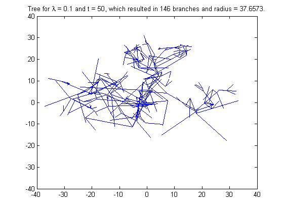
Figure 1: Simulation of $\mathcal{T}_{\lambda}(t)$ for $\mathfrak{D}=2$ with $t=50$ and $\lambda=0.1$.

2.1 Previous results

In this subsection we recall the previous mathematical results on the process $\mathcal{T}_{\lambda}$. Let $\mathcal{N}_{\lambda}(t)$ be the number of leaves of $\mathcal{T}_{\lambda}(t)$ for $t\geq 0$ (with the understanding that $\mathcal{N}_{\lambda}(0)=1$). We note that $\mathcal{N}_{\lambda}(t)$ is a birth process with birth rates $j\lambda$ for $j\in\mathbb{N}$. Thus, the following holds, see [14, Exercise 2.5.1] or [16].

Proposition 2.2.

$\mathcal{N}_{\lambda}(t)\sim\mathrm{Fs}(e^{-\lambda t})$, i.e.,

$$\mathbb{P}(\mathcal{N}_{\lambda}(t)=k)=e^{-\lambda t}(1-e^{-\lambda t})^{k-1},$$

for $k=1,2,\dots$

Thus, $\mathbb{E}[\mathcal{N}_{\lambda}(t)]=e^{\lambda t}$ and $\mathcal{N}_{\lambda}(t)$ typically grows exponentially. This is a key property which drastically changes several geometric features, compared to if the growth had been slower. Indeed, this makes sure that very rare events for a branch actually occurs all the time for the tree, changing, for example, the radius of the tree drastically, as we will see in Section 4.1.

Denote the total length of every interval in $\mathcal{T}_{\lambda}(t)$ by $\mathcal{L}_{\lambda}(t)$. The following was proved in [4, Section A.1].

Lemma 2.3.

The moment generating function $\psi_{\mathcal{L}_{\lambda}(t)}$ of $\mathcal{L}_{\lambda}(t)$ is given by

$$\psi_{\mathcal{L}_{\lambda}(t)}(x)=\frac{x-\lambda}{xe^{(\lambda-x)t}-\lambda}.$$

In particular,

$$\mathbb{E}[\mathcal{L}_{\lambda}(t)]=\frac{e^{\lambda t}-1}{\lambda}.$$

Denote by $\mathcal{A}_{r}^{\lambda}(t)=\mathrm{Area}(\{x\in\mathbb{R}^{2}:\mathrm{dist}(x,\mathcal{T}_{\lambda}(t))\leq r\})$. It is easy to see that

$$\pi r^{2}\leq\mathcal{A}_{r}^{\lambda}(t)\leq 2r\mathcal{L}_{\lambda}(t)+\frac{\pi r^{2}}{2}(\mathcal{N}_{\lambda}(t)+1).$$

We will see that the probability that $\pi/4\leq\mathcal{A}_{r}^{\lambda}(1)\leq\pi(1+r)^{2}$ converges exponentially fast to $1$ as $\lambda\to\infty$, for any value of $r>0$. Also, a functional equation for the function $q_{r}^{\lambda}(t,x)=\mathbb{P}(\mathrm{dist}(\mathcal{T}_{\lambda}(t),x)>r)$ was derived in [4, Section 3.2], but this will be stated in Section 4.2.

2.2 Differences in the model compared to previous work

While the model is mostly the same, there are some key differences compared to the works [4, 3, 8]. One obvious restriction in this note is that we consider the growth of only one tree, whereas the main goal of the papers [4, 3, 8] is to study the network composed of many trees. A restriction that is in a way imposed in said papers is that the network of trees lives in a bounded region and growth of branches is killed off upon reaching the boundary of said region. We stress, however, that some properties are also derived without considering a bounded region and when only considering one tree. Finally, we mention that in [7], the author studies the model when leaves stop growing at random

Another difficulty that arises in the perspective of the above mentioned papers is the fitting of parameters to to approximate the properties of actual neuronal networks. This is an aspect that we will not consider in this paper.

2.3 Comparison to potentially similar branching processes

There are other branching processes which might seem similar at first glance. Branching Brownian motion is naturally the one of first that comes to mind and it has been studied extensively, see e.g. [5, 15, 13, 2]. However, it satisfies very different large scale behaviour. While both of the processes typically have a radius of order $t$ (recall Proposition 1.1 and see [13, Theorem 1.1]). However, deducing a scaling rule for branching Brownian motion shows that this is not the case. Indeed, if $(\mathrm{BBM}_{\lambda}(t))_{t\geq 0}$ denotes a branching Brownian motion, where the branching rate is $\lambda$ (so that ordinary branching Brownian motion is $\mathrm{BBM}_{1}$), then we have by Brownian scaling and scaling of exponential random variables, that $\sqrt{\lambda}\mathrm{BBM}_{\lambda}(t)$ has the same law as $\mathrm{BBM}_{1}(\lambda t)$. Then, by [13, Theorem 1.1], the radius of $\mathrm{BBM}_{\lambda}(t)$ has order $\sqrt{2\lambda}t$ (plus a logarithmic term), so that increasing $\lambda$ pushes the maximal displacement of branching Brownian motion further from the origin. In the model $\mathcal{T}_{\lambda}(t)$, the same does not hold true, as $\mathcal{T}_{\lambda}(t)\subset\overline{B(0,t)}$ for any $\lambda\geq 0$.

One might also consider branching random walks, for which one has good control of the speed of growth (or in fact speeds of growth, see e.g. [6]). However, typically when studying branching random walks, one is concerned with what happens at a certain step, whereas in the present model, the number of steps taken at a finite time $t>0$ depends on the length of the steps, adding extra difficulty which to our best knowledge is not considered before in this context.

3 Branches and their approximate projections

We now give two equivalent definitions of a stochastic process which describes the law of a branch of $\mathcal{T}_{\lambda}(t)$. We denote by $\mathrm{U}(\mathcal{S}^{\mathfrak{D}-1})$ the uniform distribution on $\mathcal{S}^{\mathfrak{D}-1}$.

Definition 3.1.

Let $t_{i}\in\mathrm{Exp}(\lambda)$ and $\nu_{i}\in\mathrm{U}(\mathcal{S}^{\mathfrak{D}-1})$ for $i\in\mathbb{N}$. Define a random process $\mathcal{B}_{\lambda}(t):=(\mathcal{B}_{1}^{\lambda}(t),\mathcal{B}_{2}^{\lambda}(t))$

$$\mathcal{B}_{\lambda}(t):=(\mathcal{B}_{1}^{\lambda}(t),\dots,\mathcal{B}_{\mathfrak{D}}^{\lambda}(t))=\sum_{i=0}^{N_{\mathcal{B}}(t)}t_{i}\nu_{i}+\left(t-\sum_{i=0}^{N_{\mathcal{B}}(t)}t_{i}\right)\nu_{N_{\mathcal{B}}(t)+1}$$

where $N_{\mathcal{B}}(t):=\min\{j\geq 0:\sum_{i=0}^{j}t_{i}\leq t<\sum_{i=0}^{j+1}t_{i}\}$.

The second definition is the following.

Definition 3.2.

Let $N_{\mathcal{B}}(t)$ be a Poisson process with intensity $\lambda$ and define a random process $\mathcal{B}_{\lambda}(t):=(\mathcal{B}_{1}^{\lambda}(t),\mathcal{B}_{2}^{\lambda}(t))$

$$\mathcal{B}_{\lambda}(t):=(\mathcal{B}_{1}^{\lambda}(t),\dots,\mathcal{B}_{\mathfrak{D}}^{\lambda}(t))=\sum_{i=0}^{N_{\mathcal{B}}(t)}t_{i}\nu_{i}$$

where, conditionally on $N_{\mathcal{B}}(t)=n$, $t_{0}$ is the time of the first jump of $N_{\mathcal{B}}(t)$ and $t_{i}$ is the time between the $i$th and the $i+1$st jump of $N_{\mathcal{B}}(t)$, for $i\in\{1,...,n-1\}$ and $t_{n}=t-\sum_{i=0}^{n-1}t_{i}$.

Figure 2: Left: Simulation of $\mathcal{B}_{\lambda}(t)$ for $\mathfrak{D}=2$, with $t=20$ and $\lambda=2$. Right: Simulation of $\mathcal{B}_{\lambda}(t)$ for $\mathfrak{D}=2$, with $t=2\times 10^{6}$ and $\lambda=2$. .

However, studying the above sums is not straightforwars at all, as the number of summands depends on the magnitude of the $t_{i}$’s. In studying a branch of $\mathcal{T}_{\lambda}(t)$, it might be easier to consider the simpler process, $(X_{k})_{k\in\mathbb{N}}=(X_{k}^{1},\dots,X_{k}^{\mathfrak{D}})_{k\in\mathbb{N}}$, defined by

$$X_{k}^{n}\coloneqq\sum_{i=0}^{k}t_{i}\nu_{i}^{n},$$

where $(t_{i})$ and $(\nu_{i})$ are independent sequences such that $t_{i}\in\mathrm{Exp}(\lambda)$ and $\nu_{i}=(\nu_{i}^{1},\dots,\nu_{i}^{\mathfrak{D}})\sim\mathrm{U}(\mathcal{S}^{\mathfrak{D}-1})$ for all integers $i\geq 1$ and the $t_{i}$ (resp. $\nu_{i}$) is independent of $t_{j}$ (resp. $\nu_{j}$) whenever $j\neq i$. Let $\mathscr{F}_{k}=\sigma(t_{j},\nu_{j}:1\leq j\leq k)$. For each $n=1,\dots,\mathfrak{D}$, the process $(X_{k}^{n})_{k\in\mathbb{N}}$ will, when rescaled properly, behave approximately as the projection of a rescaled branch onto the $n$th coordinate axis. We will begin by stating some basic properties which are straightforward to check.

Lemma 3.3.

We have that

1. $\mathbb{E}[X_{k}^{n}]=0$

2. $\mathrm{Var}[X_{k}^{n}]\leq\frac{2(k+1)}{\lambda^{2}}$

3. $X_{k}^{m}$ and $X_{k}^{n}$ are uncorrelated for $m\neq n$.

4. $X_{k}^{n}$ is a martingale with respect to the filtration $(\mathscr{F}_{k})_{k\geq 1}$.

Suppose that $X_{k}=(X_{k}^{1},\dots,X_{k}^{\mathfrak{D}})$, then we would like to know the radius of $X_{k}$, i.e.,

$$R_{X}(k)=\max_{j\leq k}|X_{j}|=\max_{j\leq k}\left(\sum_{i=0}^{\mathfrak{D}}(X_{j}^{i})^{2}\right)^{1/2}.$$

It might, however, be simpler to look at $R_{X}(k)^{2}=\max_{j\leq k}\sum_{n=1}^{\mathfrak{D}}(X_{j}^{n})^{2}$. We note that if $R_{X}^{n}(k)=\max_{j\leq k}|X_{j}^{n}|$, then

$$\max_{1\leq n\leq\mathfrak{D}}R_{X}^{n}(k)\leq R_{X}(k)\leq\sum_{n=1}^{\mathfrak{D}}R_{X}^{n}(k).$$

The above observations will be used to describe the behaviour of a branch $\mathcal{B}_{\lambda}$ when $\lambda\to\infty$.

Lemma 3.4.

For each $t>0$, the branch $(\mathcal{B}_{\lambda}(s))_{0\leq s\leq t}$ converges to $(0,0)$ in probability with respect to the Hausdorff topology as $\lambda\to\infty$. That is, the random variable $\max_{0\leq s\leq t}|\mathcal{B}_{\lambda}(s)|$ converges to $0$ in probability as $\lambda\to\infty$.

Proof.

We begin by noting that we can couple $\mathcal{B}_{\lambda}$ with $(X_{j})_{j\in\mathbb{N}}$ so that if $(t_{j})_{j\in\mathbb{N}}$ are the times between the changes of direction in the branch $\mathcal{B}_{\lambda}$ and $t_{k}^{*}=\sum_{j\leq k}t_{j}$ are the times at which the changes are made, then $\mathcal{B}_{\lambda}(t_{k}^{*})=X_{k}$, and such that the direction that the branch grows in a given time interval is the same as that of $X$ in the corresponding one. That is, the processes $\mathcal{B}_{\lambda}$ and $(X_{j})_{j\in\mathbb{N}}$ change direction at the same times and the growth directions are the same. We note that for each $k\in\mathbb{N}$.

$$\max_{0\leq s\leq t_{k}^{*}}|\mathcal{B}_{\lambda}(s)|=\max_{j\leq k}|\mathcal{B}_{\lambda}(t_{j}^{*})|=R_{X}(k).$$ (3.1)

For $n=1,\dots,\mathfrak{D}$, we have by the Kolmogorov martingale inequality and Lemma 3.3, that

$$\mathbb{P}(R_{X}^{n}(k)\geq\varepsilon)\leq\max_{j\leq k}\frac{\mathrm{Var}(X_{k}^{n})}{\varepsilon}\leq\frac{2(k+1)}{\varepsilon\lambda^{2}}.$$ (3.2)

Consequently,

$$\mathbb{P}(R_{X}(k)\geq\varepsilon)\leq\sum_{n=1}^{\mathfrak{D}}\mathbb{P}(R_{X}^{n}(k)\geq\varepsilon/\mathfrak{D})\leq\frac{2\mathfrak{D}^{2}(k+1)}{\varepsilon\lambda^{2}}.$$ (3.3)

Let $N_{\mathcal{B}}(t)$ be as in Definition 3.1 and recall that $N_{\mathcal{B}}(t)\sim\mathrm{Po}(\lambda t)$. Thus, we have that

$$\mathbb{P}\!\left(\max_{0\leq s\leq t}|\mathcal{B}_{\lambda}(s)|\geq\varepsilon\right)\leq\mathbb{P}(R_{X}(k)\geq\varepsilon)+\mathbb{P}(N_{\mathcal{B}}(t)>k).$$ (3.4)

Next we note that for any integer $k>\lambda t$, we have by a Chernoff bound that

$$\mathbb{P}(N_{\mathcal{B}}(t)\geq k)\leq\frac{(e\lambda t)^{k}e^{-\lambda t}}{k^{k}},$$ (3.5)

and hence, choosing $k=\lceil(\lambda t)^{3/2}\rceil$, we have by (3.3), (3.4) and (3.5) that

$$\mathbb{P}\!\left(\max_{0\leq s\leq t}|\mathcal{B}_{\lambda}(s)|\geq\varepsilon\right)=O(\lambda^{-1/2}).$$

Thus $\max_{0\leq s\leq t}|\mathcal{B}_{\lambda}(s)|\to(0,0)$ in probability as $\lambda\to\infty$ and hence the proof is done. ∎

For more on the processes $X$ and $\mathcal{B}_{\lambda}$ in the case $\mathfrak{D}=2$, see [16].

4 On the geometry of $\mathcal{T}_{\lambda}(t)$

In this section, we study the geometry of the tree $\mathcal{T}_{\lambda}(t)$. We begin by noting the following scaling relation, which is the key observation for the proofs of the present paper.

Lemma 4.1.

Fix $t_{0}>0$. Then, $\tfrac{t_{0}}{t}\mathcal{T}_{\lambda}(t)$ and $\mathcal{T}_{\lambda t/t_{0}}(t_{0})$ have the same law. In particular, $\mathcal{T}_{\lambda}(t)/t$ and $\mathcal{T}_{\lambda t}(1)$ have the same law.

Proof.

This follows since if $t_{i}\sim\mathrm{Exp}(\lambda)$, then $t_{i}/t\sim\mathrm{Exp}(\lambda t)$. ∎

Thus, in studying $\mathcal{T}_{\lambda}(t)$ for large $t$, we can (for some properties) instead study $\mathcal{T}_{\lambda}(1)$ for large intensity. Note here that any behaviour that is of scale $o(t)$, such as lower order radius terms or possibly fluctuations of the outer boundary, will not show up when rescaling as above.

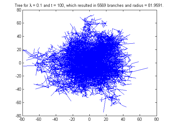
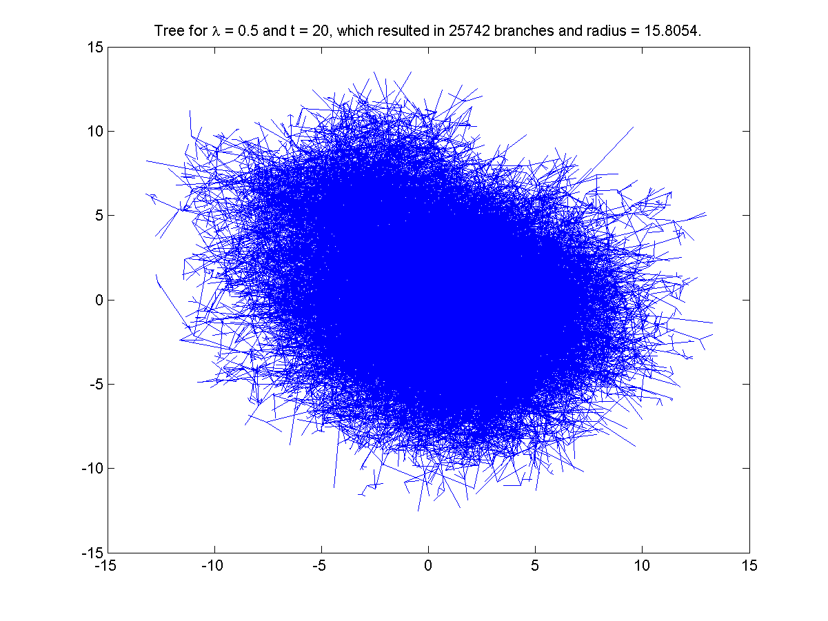
Figure 3: Left: Simulation of $\mathcal{T}_{\lambda}(t)$ for $\mathfrak{D}=2$, with $t=100$ and $\lambda=0.1$. Right: Simulation of $\mathcal{T}_{\lambda}(t)$ for $\mathfrak{D}=2$, with $t=20$ and $\lambda=0.5$. Note that by Lemma 4.1, the laws of the simulations are the same, up to scaling the tree by $5$.

4.1 Radius of the tree

Let $\mathcal{R}_{\lambda}(t)=\mathrm{rad}\,\mathcal{T}_{\lambda}(t)=\sup_{x\in\mathcal{T}_{\lambda}(t)}|x|$ denote the radius of $\mathcal{T}_{\lambda}(t)$. It is natural to consider the asymptotics of $\mathcal{R}_{\lambda}(t)$ as $t\to\infty$ and by virtue of Lemma 4.1 (which implies that $\mathcal{R}_{\lambda}(t)/t$ and $\mathcal{R}_{\lambda t}(1)$ have the same law), we may instead study $\mathcal{R}_{\lambda}(1)$ as $\lambda\to\infty$. We begin by noting that the law of $\mathcal{R}_{\lambda}(t)$ is continuous in $\lambda$.

Lemma 4.2.

For each $t,r>0$, the function $\lambda\mapsto\mathbb{P}(\mathcal{R}_{\lambda}(t)\leq r)$ is continuous for all $t,r>0$.

Proof.

By Lemma 4.1, $\mathcal{R}_{\lambda}(t)$ has the same law as $\mathcal{R}_{1}(\lambda t)/\lambda$, which is almost surely a continuous function of $\lambda\in(0,\infty)$ for each fixed $t>0$. To see that $\mathcal{R}_{\lambda}(t)$ is continuous at $\lambda=0$, note that $\mathbb{P}(\text{no branching occurs before time}\ t)=\mathbb{P}(\mathrm{Exp}(\lambda)>t)=e^{-\lambda t}\to 1$ as $\lambda\to 0$. ∎

Next we note the following immediate consequence of Lemma 4.1, namely that any limit of $\mathcal{R}_{\lambda}(t)/t$ is independent of $\lambda$. Note, however, that this could at this stage very well not mean anything, as it is not yet clear that $\mathcal{R}_{\lambda}(t)$ is not of order $o(t)$, as a typical branch is.

Lemma 4.3.

The laws of $\liminf_{t\to\infty}\mathcal{R}_{\lambda}(t)/t$ and $\limsup_{t\to\infty}\mathcal{R}_{\lambda}(t)/t$ do not depend on $\lambda$.

Proof.

Follows immediately from Lemma 4.1. ∎

Now, we shall lower bound the radius of the tree. Seeing as a branch will converge to the point $(0,0)$ as $\lambda\to\infty$ (by Lemma 3.4), it might seem reasonable to expect $\mathcal{R}_{\lambda}(1)$ to decrease to $0$ as $\lambda\to\infty$ as well. However, we shall see that the sheer number of branches forces the radius of the tree to be positive.

Proposition 4.4.

For each $\varepsilon>0$, we have that

$$\mathbb{P}(\mathcal{R}_{\lambda}(1)\leq 1/2-\varepsilon)=O(e^{-\varepsilon\lambda/2}),$$

where the implicit constant can be taken to be independent of $\varepsilon$.

Proof.

Note that by Proposition 2.2 and Lemma A.1,

$$\mathbb{P}(\mathcal{N}_{\lambda}((1+\varepsilon)/2)\leq e^{\lambda/2})\leq\sum_{n=1}^{\infty}\frac{e^{-n\lambda/2}}{n}\leq Ce^{-\varepsilon\lambda/2},\quad\text{as}\quad\lambda\to\infty,$$

where $C>0$ is some universal constant. Thus, with probability at least $1-Ce^{-\varepsilon\lambda/2}$, there are at least $e^{\lambda/2}$ leaves at time $(1+\varepsilon)/2$. Moreover, if the tree branches at the point $x\in B(0,(1+\varepsilon)/2)$, then there is a neighbourhood $U_{\varepsilon}$ of $x/|x|$ in $\mathcal{S}^{\mathfrak{D}-1}$ such that if a branch grows in the direction of $\nu_{\varepsilon}\in U_{\varepsilon}^{x}$ for time at least $(1-\varepsilon)/2$ from $x$ before branching, then $\mathcal{R}_{\lambda}(1)\geq 1/2-\varepsilon$ and by standard geometry, the probability that a vector with law $\mathrm{U}(\mathcal{S}^{\mathfrak{D}-1})$ belongs to $U_{\varepsilon}^{x}$ is at least a constant (depending only on $\mathfrak{D}$) times $\varepsilon^{\mathfrak{D}/2}$.We say that a branch growing from the point $x$ grows in an $\varepsilon$-optimal direction if the direction in which it grows belongs to $U_{\varepsilon}^{x}$. Assuming that we are on the event that $\mathcal{N}_{\lambda}((1+\varepsilon)/2)\geq e^{\lambda/2}$, we have by Hoeffding’s bound, that the conditional probability that fewer than $\varepsilon^{\mathfrak{D}}e^{\lambda/2}$ of the (at least) $e^{\lambda/2}$ active ends are growing in the the $\varepsilon$-optimal direction is upper bounded by $\exp(-\varepsilon^{\mathfrak{D}}e^{\lambda/2})$. On the event that at least $\varepsilon^{\mathfrak{D}}e^{\lambda/2}$ leaves at time $(1+\varepsilon)/2$ are growing in the $\varepsilon$-optimal direction, we have by the memoryless property of the exponential distribution and Lemma A.2, that the conditional probability that none of the $\varepsilon^{\mathfrak{D}}e^{\lambda/2}$ leaves produces an interval of length at least $(1-\varepsilon)/2$, is at most $C_{1}\exp(-C_{0}e^{\varepsilon\lambda/2})$. Hence, we have that

$$\mathbb{P}(\mathcal{R}_{\lambda}(1)\geq 1/2-\varepsilon)\geq(1-Ce^{-\varepsilon\lambda/2})\times(1-\exp(-\varepsilon^{\mathfrak{D}}e^{\lambda/2}))\times(1-C_{1}\exp(-C_{0}e^{\varepsilon\lambda/2}))=1-O(e^{-\varepsilon\lambda/2}),$$

which concludes the proof. ∎

Next, we prove a $0$-$1$-type result.

Lemma 4.5.

Fix $d\in[0,1]$. If there exists $p>0$ and $\lambda_{0}>0$ such that $\mathbb{P}(\mathcal{R}_{\lambda}(1)\geq d)\geq p$ for all $\lambda\geq\lambda_{0}$, then for $a\in(0,1)$,

$$\mathbb{P}(\mathcal{R}_{\lambda}(1)\leq d-\delta)=O(e^{-a\lambda\delta/2}),$$

where the implicit constant can be taken to be universal.

Proof.

By the assumption of the lemma and Lemma 4.1, we have that if $\delta>0$, then

$$\mathbb{P}(\mathcal{R}_{\lambda}(1-\delta/2)\geq d-\delta/2)\geq p,$$ (4.1)

for all $\lambda\geq\lambda_{0}/(1-\delta/2)$ and that if any descending tree of a point in $\mathcal{T}_{\lambda}(\delta/2)$ has radius at least $d-\delta/2$ within time $1-\delta/2$ of its starting time, then $\mathcal{R}_{\lambda}(1)\geq d-\delta$. Moreover, for fixed $a\in(0,1)$, we note that by Lemma A.1,

$$\mathbb{P}(\mathcal{N}_{\lambda}(\delta/2)\geq e^{(1-a)\lambda\delta/2})\geq 1-O(e^{-a\lambda\delta/2}).$$ (4.2)

By (4.1), we have the following lower bound on the conditional probability that that $\mathcal{R}_{\lambda}(1)\geq d-\delta$ given the event $\{\mathcal{N}_{\lambda}(\delta/2)\geq e^{(1-a)\lambda\delta/2}\}$,

$$\mathbb{P}(\mathcal{R}_{\lambda}(1)\geq d-\delta\,|\,\mathcal{N}_{\lambda}(\delta/2)\geq e^{(1-a)\lambda\delta/2})\geq 1-(1-p)^{\exp((1-a)\lambda\delta/2)}.$$ (4.3)

Consequently, by (4.2) and (4.3), we have that

$$\mathbb{P}(\mathcal{R}_{\lambda}(1)\geq d-\delta)=1-O(e^{-a\lambda\delta/2}),$$ (4.4)

where the implicit constant can be taken to be universal. Thus the proof is complete. ∎

Corollary 4.6.

Suppose that $d,p,\lambda_{0}>0$ are such that $\mathbb{P}(\mathcal{R}_{\lambda}(1)\geq d)\geq p$ for all $\lambda\geq\lambda_{0}$. Then, almost surely,

$$\liminf_{t\to\infty}\mathcal{R}_{\lambda}(t)/t\geq d.$$

Proof.

For $k\in\mathbb{N}$ we consider the event $E_{k}=\{\mathcal{R}_{\lambda}(k)/k\leq d-\varepsilon\}$. We note that if $E_{k}$ does not occur, then

$$\frac{\mathcal{R}_{\lambda}(t)}{t}\geq\left(d-\varepsilon\right)\frac{k}{k+1},\quad k\leq t\leq k+1.$$ (4.5)

Let $F_{k}=\{\exists j\geq k:E_{j}\ \text{occurs}\}$ and note that by (4.5), we have for each $k\in\mathbb{N}$ that

$$\left\{\liminf_{t\to\infty}\mathcal{R}_{\lambda}(t)/t\leq(d-\varepsilon)\tfrac{k}{k+1}\right\}\subset F_{k}.$$

Moreover, we note that $F_{k}\subset\cup_{j\geq k}E_{j}$ and by Lemma 4.5 with, say, $a=1/2$, we have

$$\mathbb{P}(E_{k})=\mathbb{P}(\mathcal{R}_{k\lambda}(1)\leq d-\varepsilon)\lesssim e^{-k\varepsilon\lambda/4},$$

where the implicit constant is universal. Consequently,

$$\mathbb{P}(F_{k})\leq\sum_{j\geq k}\mathbb{P}(E_{j})\lesssim\sum_{j\geq k}e^{-j\varepsilon\lambda/4}\lesssim e^{-k\varepsilon\lambda/4},$$

where the implicit constants depend only on $\lambda$ and $\varepsilon$ and hence $\mathbb{P}(\liminf_{t\to\infty}\mathcal{R}_{\lambda}(t)/t<d-\varepsilon)=0$. Since $\varepsilon>0$ was arbitrary, the result follows. ∎

Proofs of first parts of Propositions 1.1 and 1.3.

The first part of Proposition 1.1 are collected in Proposition 4.4, Corollary 4.6 and Lemma 4.3. The first part of Proposition 1.3 is just Proposition 4.4. ∎

4.2 Connection probabilities

Fix some point $x\in\mathbb{R}^{\mathfrak{D}}$. Let

$$p_{r}^{\lambda}(t,x)\coloneqq\mathbb{P}(\mathrm{dist}(\mathcal{T}_{\lambda}(t),x)\leq r),$$

and note that $p_{r}^{\lambda}(t,x)$ is radially symmetric in $x$, that is, its dependence on $x$ is only on $|x|$. Thus, we may and will sometimes write $p_{r}^{\lambda}(t,d)$ when $|x|=d$. Furthermore, we let

$$q_{r}^{\lambda}(t,x)=\mathbb{P}(\mathrm{dist}(\mathcal{T}_{\lambda}(t),x)>r)=1-p_{r}^{\lambda}(t,x).$$

Assume for now that $\mathfrak{D}=2$. Then, we have from [4, Section 3.2], the following functional equation for $q_{r}^{\lambda}(t,x)$. For $|x|=d$, $t>d-r$ and $d>r$,

$$q_{r}^{\lambda}(t,d)= \int_{-\alpha_{0}}^{\alpha_{0}}\int_{0}^{s_{0}(\alpha)}\frac{\lambda e^{-\lambda s}}{2\pi}q_{r}^{\lambda}(t-s,D(s,\alpha))^{2}dsd\alpha$$

$$+\int_{\alpha_{0}}^{2\pi-\alpha_{0}}\int_{0}^{t}\frac{\lambda e^{-\lambda s}}{2\pi}q_{r}^{\lambda}(t-s,D(s,\alpha))^{2}dsd\alpha+e^{-\lambda t}f_{r}^{\lambda}(t,d),$$ (4.6)

where $\alpha_{0}=\arcsin\tfrac{r}{d}$, $s_{0}(\alpha)=d\cos\alpha-\sqrt{r^{2}-d^{2}\sin^{2}\alpha}$, $D(s,\alpha)=\sqrt{d^{2}+s^{2}-2ds\cos\alpha}$, and

$$f_{r}^{\lambda}(t,d) =\mathbb{P}(\mathrm{dist}(\mathcal{T}_{\lambda}(t),x)>r\,|\,\textup{no branching has occurred before time}\,t)$$

$$=\begin{cases}1-\frac{1}{\pi}\arccos\!\left(\frac{d^{2}+t^{2}-r^{2}}{2td}\right)\!,&\textup{if }d-r\leq t\leq\sqrt{d^{2}-r^{2}},\\ 1-\frac{1}{\pi}\arcsin\frac{r}{d},&\textup{if }t>\sqrt{d^{2}-r^{2}},\end{cases}$$

with boundary conditions

$$q_{r}^{\lambda}(t,d)=0,\quad\textup{if }d\leq r,\ t\geq 0,$$

$$q_{r}^{\lambda}(t,d)=1,\quad\textup{if }d>r,\ 0\leq t<d-r.$$

While this does not yield an analytic solution, it does allow for numerical computation. Similar equations can be derived in any dimension. For the case $\mathfrak{D}=3$, see [8, Section 3.2].

Now, allowing for general $\mathfrak{D}$, we have (see [8, Equation (12)]) that

$$p_{r}^{\lambda}(t,x)\geq e^{-\lambda t}p_{r}^{0}(t,x).$$

Moreover, it is obvious from the definition that if $r_{1}\leq r_{2}$ and $t_{1}\leq t_{2}$, then

$$p_{r_{1}}^{\lambda}(t_{1},x)\leq p_{r_{2}}^{\lambda}(t_{2},x).$$ (4.7)

Using Lemma 4.1, we have the following identities. Let $t_{0}>0$ and $d=|x|$. Then,

$$p_{r}^{\lambda}(t,x)=p_{rt_{0}/t}^{\lambda t/t_{0}}(t_{0},xt_{0}/t)=p_{r/t}^{\lambda t}(1,x/t)=p_{r/d}^{\lambda d}(t/d,1).$$ (4.8)

Let $a>1$ and note that by (4.7) and (4.8),

$$p_{r}^{\lambda}(t,x)\leq p_{r}^{a\lambda}(t,x/a).$$

We expect that in the variables $\lambda$ and $x$, the functions $p_{r}^{\lambda}(t,x)$ do not display the same monotonicity. Indeed, one can expect that for $x$ close to $0$, $\lambda_{1}\leq\lambda_{2}$ implies that $p_{r}^{\lambda_{1}}(t,x)\leq p_{r}^{\lambda_{2}}(t,x)$ (since if the first branch misses the ball $B(x,r)$, then a larger branching intensity gives the tree more “attempts” at hitting it). On the other hand, we know that the conditional probability that $\mathcal{R}_{\lambda}(t)=t$ given that a branching occurs is zero, so the maximal radius is only attained if the tree never branches, which is more likely to occur if $\lambda$ is smaller. Hence, it is reasonable to expect that $p_{r}^{\lambda_{1}}(t,x)\geq p_{r}^{\lambda_{2}}(t,x)$ for $x$ close to $\partial B(0,t)$ and $r$ small, whenever $\lambda_{1}$ and $\lambda_{2}$ are small. But for large $\lambda_{1}$ and $\lambda_{2}$, it seems reasonable to expect that the increase in the number of branches is what will impact the connection probability the most. In other words, for $x$ close to $\partial B(0,t)$, we expect that $\lambda\mapsto p_{r}^{\lambda}(t,x)$ is decreasing on some interval $[0,\lambda_{0}]$ and then increasing on $[\lambda_{0},\infty)$.

Remark 4.7.

For $r>0$, $\lambda>0$, $x\in\mathfrak{D}$ and $t>0$, let $\mathcal{N}_{r}^{\lambda}(t,x)=|\mathcal{S}_{\lambda}(t)\cap B(x,r)|$, that is, $\mathcal{N}_{r}^{\lambda}(t,x)$ is the number of branching points of $\mathcal{T}_{\lambda}(t)$ that lie in $B(x,r)$, and let $\mathscr{N}_{r}^{\lambda}(t,x)=\mathbb{E}[\mathcal{N}_{r}^{\lambda}(t,x)]$. Then, similarly to the above, one can derive a functional equation for $\mathscr{N}_{r}^{\lambda}(t,x)$, see [7]. Moreover, for $D\subset\mathbb{R}^{\mathfrak{D}}$, $\mathcal{L}_{\lambda}(t,D)$ be the total length of the intervals of $\mathcal{T}_{\lambda}(t)\cap D$. If we write $\ell_{r}^{\lambda}(t,x)=\mathbb{E}[\mathcal{L}_{\lambda}(t,B(x,r))]$, then in the same way one can derive a functional equation for it. Moreover, similarly to the equations for $q_{r}^{\lambda}(t,x)$, the equations for $\mathscr{N}_{r}^{\lambda}(t,x)$ and $\ell_{r}^{\lambda}(t,x)$ do not give us analytic solutions, but could be used for numerical computations.

4.2.1 Connection probabilities as $\lambda\to\infty$

Again, let us first focus on the case $\mathfrak{D}=2$. We would like to consider $p_{r}^{\infty}(t,d)=\lim_{\lambda\to\infty}p_{r}^{\lambda}(t,d)$, provided that the limit exists. Equivalently, we can consider $q_{r}^{\infty}(t,d)=\lim_{\lambda\to\infty}q_{r}^{\lambda}(t,d)$ (provided that the limit exists). For now, assume that the limit exists (in some sufficiently good sense).

We note that if $\mathfrak{f}_{\lambda}(s)=\lambda e^{-\lambda s}$, then $\mathfrak{f}_{\lambda}\to\delta_{0}$ in the space of tempered distributions on the Schwartz space as $\lambda\to\infty$. In a space of distributions over a slightly more general function space (allowing for discontinuities), $\mathfrak{f}_{\lambda}\to\delta_{0+}$ where $\delta_{0+}$ is the distribution acting on functions as $\delta_{0+}[\varphi]=\lim_{x\searrow 0}\varphi(x)$. Thus, taking the limit as $\lambda\to\infty$ in (4.2) it is reasonable to expect that

$$q_{r}^{\infty}(t,d)=q_{r}^{\infty}(t,d)^{2},$$

that is, $q_{r}^{\infty}(t,d)\in\{0,1\}$, whenever $(t,d)$ is a continuity point of $q_{r}^{\infty}$. The same analysis can be carried out in the case $\mathfrak{D}=3$. Next we prove that there is at least an interval of $d$ where it is true for arbitrary dimension $\mathfrak{D}$ (and we expect the statement to be true for all $d$).

Proposition 4.8.

Suppose that $d,p,\lambda_{0}>0$ are such that $\mathbb{P}(\mathcal{R}_{\lambda}(1)\geq d)\geq p$ for all $\lambda\geq\lambda_{0}$. Then, $p_{r}^{\lambda}(1,x)\to 1$ exponentially fast as $\lambda\to\infty$, whenever $|x|-r<d$.

Remark 4.9.

Proposition 4.8 essentially states that as $\lambda\to\infty$, the entire ball $B(0,d)$ will be filled by $\mathcal{T}_{\lambda}(1)$ and hence that if $B(x,r)\cap B(0,d)\neq\emptyset$, then $\mathcal{T}_{\lambda}(1)\cap B(x,r)\neq\emptyset$.

Proof of Proposition 4.8.

In order to prove the convergence in the case of $p_{r}^{\lambda}(1,x)$, where $|x|-r<d$, it suffices to prove it with $\widetilde{x}$ and $\widetilde{r}$ such that $B(\widetilde{x},\widetilde{r})\subset B(0,d)$ in place of general $x$ and $r$ (since $B(x,r)\cap B(0,d_{0})$ contains such a ball).

By the above reason and symmetry, we consider $x\in(0,1)$ and $r$ such that $B(x,r)\subset B(0,d)$ and we let $\delta\coloneqq(d-x)\wedge 1/100$. For a fixed $a\in(0,1)$ we have by (4.4) and symmetry that there is some universal constant $c>0$ such that

$$\mathbb{P}(\mathrm{dist}(\mathcal{T}_{\lambda}(1-\delta/2),y)\leq r)\geq cr^{\mathfrak{D}-1}-O(e^{-a\lambda\delta(1-d)/(2-\delta)}),$$

for all $y\in B(0,d-\delta/2)$. Thus, arguing as in the proof of Lemma 4.5, we have that

$$p_{r}^{\lambda}(1,x)\geq 1-O(e^{-a\lambda\delta(1-d)/(2-\delta)}).$$ (4.9)

∎

The statement of Proposition 4.8 essentially says that there is a ball centred at $0$ which gets filled by the tree $\mathcal{T}_{\lambda}(1)$ as $\lambda\to\infty$. When translating this to the case of $\mathcal{T}_{\lambda}(t)$ via scaling (Lemma 4.1) this would then tell us that, while the process $\mathcal{T}_{\lambda}(t)$ may not have the same sharp behaviour as $t\to\infty$, it would roughly be a disk of radius $td$, where each point is at most distance $o(t)$ from $\mathcal{T}_{\lambda}(t)$ for large $t$.

Proposition 4.10.

Suppose that $d,p,\lambda_{0}>0$ are such that $\mathbb{P}(\mathcal{R}_{\lambda}(1)\geq d)\geq p$ for all $\lambda\geq\lambda_{0}$. Then $\mathcal{T}_{\lambda}(1)\cap B(0,d)\to B(0,d)$ in probability with respect to the Hausdorff topology as $\lambda\to\infty$.

Proof.

Let $X_{\varepsilon}=(\tfrac{\varepsilon}{2}\mathbb{Z}^{\mathfrak{D}})\cap B(0,d-\varepsilon/4)$ and note that if $\mathrm{dist}(\mathcal{T}_{\lambda}(1),x)\leq\varepsilon$ for each $x\in X_{\varepsilon}$, then $\mathrm{dist}_{H}(\mathcal{T}_{\lambda}(1),B(0,d))\leq\varepsilon$, where $\mathrm{dist}_{H}$ denotes the Hausdorff distance. Thus, fixing some $a\in(0,1)$, we have by the estimate (4.9), that

$$\mathbb{P}(\mathrm{dist}_{H}(\mathcal{T}_{\lambda}(1),B(0,d))>\varepsilon) \leq\mathbb{P}(\exists x\in X_{\varepsilon}:\mathrm{dist}(\mathcal{T}_{\lambda}(1),x)>\varepsilon/2)\leq\sum_{x\in X_{\varepsilon}}\mathbb{P}(\mathrm{dist}(\mathcal{T}_{\lambda}(1),x)>\varepsilon)$$

$$\lesssim\varepsilon^{-2\mathfrak{D}}\times O(e^{-a\lambda\varepsilon(1-d)/4}),$$ (4.10)

where the implicit constant may depend on $\varepsilon$, but not $\lambda$. Thus, as $\lambda\to\infty$, (4.2.1) decays to $0$. Since $\varepsilon>0$ was arbitrary, the proof is done. ∎

We record the following estimate that came from the above proof.

Lemma 4.11.

Suppose that $d,p,\lambda_{0}>0$ are such that $\mathbb{P}(\mathcal{R}_{\lambda}(1)\geq d)\geq p$ for all $\lambda\geq\lambda_{0}$. Then,

$$\mathbb{P}(\exists x\in B(0,td):\mathrm{dist}(\mathcal{T}_{\lambda}(t),x)>\varepsilon t)=O(e^{-t(a\lambda(1-d)/4+o(1))}).$$

Remark 4.12.

In the functional equations mentioned in Remark 4.7, the same procedure as above (letting $\lambda\to\infty$), does not indicate any nontrivial behaviour. Indeed, it is obvious that the number of branching points and total length in a ball will be either $0$ (if the tree does not intersect it) or infinite (if the tree hits the ball, then as $\lambda\to\infty$, the number of branching points occurring in said ball will grow exponentially with $\lambda$ and hence the number of intervals as well. This is reflected, for example, in the functional equation essentially turning into the equation $\ell_{r}^{\infty}(t,d)=2\ell_{r}^{\infty}(t,d)$ as $\lambda\to\infty$, and hence that $\ell_{r}^{\infty}(t,d)\in\{0,\infty\}$.

Proofs of last parts of Propositions 1.1 and 1.3.

The last part of Proposition 1.1 is stated in Lemma 4.11 and the last part of Proposition 1.3 is given in Proposition 4.10. ∎

Appendix A Asymptotics of first success and exponential distributions

In this appendix we prove the necessary asymptotics for first success and exponential distributions, that are used to prove the radius bounds in Section 4.1. For each $y\in(0,1)$, let $N_{y}\sim\mathrm{Fs}(y)$.

Lemma A.1.

We have that $yN_{y}\to\mathrm{Exp}(1)$ in distribution as $y\to 0$. Moreover, if $0<a<1$ and $b>0$, then

$$\mathbb{P}(N_{y}\leq by^{-a})\leq b\sum_{n=1}^{\infty}\frac{y^{n-a}}{n}.$$ (A.1)

Proof.

Fix $0<a\leq 1$ and $b>0$, and recall that $\log(1-y)=-\sum_{n=1}^{\infty}y^{n}/n$ whenever $|y|<1$. We have that

$$\mathbb{P}(N_{y}\leq by^{-a}) =1-(1-y)^{b/y^{a}}(1-y)^{\lfloor b/y^{a}\rfloor-b/y^{a}}$$

$$=1-e^{by^{-a}\log(1-y)}(1-y)^{\lfloor b/y^{a}\rfloor-b/y^{a}}$$

$$=1-\exp\!\left(-b\sum_{n=1}^{\infty}\frac{y^{n-a}}{n}\right)(1-y)^{\lfloor b/y^{a}\rfloor-b/y^{a}}$$

Since $1\leq(1-y)^{t}\leq 1/(1-y)$ whenever $-1\leq t\leq 0$, we have that

$$1-\frac{1}{1-y}\exp\!\left(-b\sum_{n=1}^{\infty}\frac{y^{n-1}}{n}\right)\leq\mathbb{P}(yN_{y}\leq b)\leq 1-e^{-b},$$

and thus $yN_{y}\to\mathrm{Exp}(1)$ in distribution. Similarly, using that $e^{-t}>1-t$ for all $t>0$, we have for $0<a<1$ that

$$\mathbb{P}(N_{y}\leq by^{-a})\leq b\sum_{n=1}^{\infty}\frac{y^{n-a}}{n}.$$

∎

For each $x>0$, let $(T_{x}^{j})_{j\in\mathbb{N}^{+}}$ be an i.i.d. collection of $\mathrm{Exp}(x)$-distributed random variables.

Lemma A.2.

Let $a>c>0$ and $b>0$. Then, there exist constants $C_{0},C_{1}>0$, depending on $a$, $b$ and $c$ such that for all $x\geq 1$,

$$\mathbb{P}\!\left(\max_{j\leq be^{ax}}\,T_{x}^{j}\leq c\right)\leq C_{1}\exp(-C_{0}e^{(a-c)x}).$$

Proof.

We have that

$$\mathbb{P}\!\left(\max_{j\leq be^{ax}}\,T_{x}^{j}\leq c\right) =\mathbb{P}(T_{x}^{1}\leq c)^{\lfloor be^{ax}\rfloor}=(1-e^{-cx})^{be^{ax}}(1-e^{-cx})^{\lfloor be^{ax}\rfloor-be^{ax}}$$

$$=\exp(be^{ax}\log(1-e^{-cx}))(1-e^{-cx})^{\lfloor be^{ax}\rfloor-be^{ax}}$$

$$=\exp\!\left(-be^{ax}\sum_{n=1}^{\infty}\frac{e^{-ncx}}{n}\right)(1-e^{-cx})^{\lfloor be^{ax}\rfloor-be^{ax}}$$

$$\asymp\exp\!\left(-be^{ax}\sum_{n=1}^{\infty}\frac{e^{-ncx}}{n}\right)$$

$$\lesssim\exp(-Ce^{(a-c)x}).$$

∎

References

- [1] J. Aćimović, T. Mäki-Marttunen, R. Havela, H. Teppola, and M.-L. Linne. Modeling of neuronal growth in vitro: Comparison of simulation tools netmorph and cx3d. EURASIP J Bioinform Syst Biol., 2011(1):616382, 2011.
- [2] E. Aïdékon, J. Berestycki, É. Brunet, and Z. Shi. Branching Brownian motion seen from its tip. Probab. Theory Related Fields, 157(1-2):405–451, 2013.
- [3] Fioralba Ajazi, Valérie Chavez-Demoulin, and Tatyana Turova. Networks of random trees as a model of neuronal connectivity. J. Math. Biol., 79(5):1639–1663, 2019.
- [4] Fioralba Ajazi, George M. Napolitano, Tatyana Turova, and Izbassar Zaurbek. Structure of a randomly grown 2-d network. Biosystems, 136:105–112, 2015. Selected papers presented at the Eleventh International Workshop on Neural Coding, Versailles, France, 2014.
- [5] Maury D. Bramson. Maximal displacement of branching Brownian motion. Comm. Pure Appl. Math., 31(5):531–581, 1978.
- [6] Nina Gantert. The maximum of a branching random walk with semiexponential increments. Ann. Probab., 28(3):1219–1229, 2000.
- [7] Vasilii Goriachkin. Critical Scaling in Particle Systems and Random Graphs. PhD thesis, Lund University, Lund, Sweden, November 2023.
- [8] Vasilii Goriachkin and Tatyana Turova. Decay of connection probabilities with distance in 2d and 3d neuronal networks. Biosystems, 184:103991, 2019.
- [9] Simon C. Harris, Emma Horton, Andreas E. Kyprianou, and Ellen Powell. Many-to-few for non-local branching Markov process. arXiv e-prints, page arXiv:2211.08662, November 2022.
- [10] Simon C. Harris and Matthew I. Roberts. The many-to-few lemma and multiple spines. Ann. Inst. Henri Poincaré Probab. Stat., 53(1):226–242, 2017.
- [11] Randal A Koene, Betty Tijms, Peter van Hees, Frank Postma, Alexander de Ridder, Ger J A Ramakers, Jaap van Pelt, and Arjen van Ooyen. Netmorph: a framework for the stochastic generation of large scale neuronal networks with realistic neuron morphologies. Neuroinformatics, 7(3):195–210, 2009.
- [12] Tuomo Mäki-Marttunen. Modelling Structure and Dynamics of Complex Systems: Applications to Neuronal Networks. PhD thesis, Tampere University, Tampere, Finland, December 2013.
- [13] Bastien Mallein. Maximal displacement of -dimensional branching Brownian motion. Electron. Commun. Probab., 20:no. 76, 12, 2015.
- [14] J. R. Norris. Markov chains, volume 2 of Cambridge Series in Statistical and Probabilistic Mathematics. Cambridge University Press, Cambridge, 1998. Reprint of 1997 original.
- [15] Matthew I. Roberts. Fine asymptotics for the consistent maximal displacement of branching Brownian motion. Electron. J. Probab., 20:no. 28, 26, 2015.
- [16] Lukas Schoug. Geometry of a random tree process. Master’s thesis, Lund University, Lund, Sweden, August 2015.