Tenplex: Changing Resources of Deep Learning Jobs
using Parallelizable Tensor Collections

Abstract

Deep learning (DL) jobs use multi-dimensional parallelism, i.e. they combine data, model, and pipeline parallelism, to use large GPU clusters efficiently. This couples jobs tightly to a set of GPU devices, but jobs may experience changes to the device allocation: (i) resource elasticity during training adds or removes devices; (ii) hardware maintenance may require redeployment on different devices; and (iii) device failures force jobs to run with fewer devices. Current DL frameworks lack support for these scenarios, as they cannot change the multi-dimensional parallelism of an already-running job in an efficient and model-independent way.

We describe Tenplex, a state management library for DL frameworks that enables jobs to change the GPU allocation and job parallelism at runtime. Tenplex achieves this by externalizing the DL job state during training as a parallelizable tensor collection (PTC). When the GPU allocation for the DL job changes, Tenplex uses the PTC to transform the DL job state: for the dataset state, Tenplex repartitions it under data parallelism and exposes it to workers through a virtual file system; for the model state, Tenplex obtains it as partitioned checkpoints and transforms them to reflect the new parallelization configuration. For efficiency, these PTC transformations are executed in parallel with a minimum amount of data movement between devices and workers. Our experiments show that Tenplex enables DL jobs to support dynamic parallelization with low overhead.

1 Introduction

Deep learning (DL) has led to remarkable progress in many domains, including conversational AI [40], natural language processing [9, 6, 20], computer vision [21, 59], and recommender systems [70, 17]. These advances, however, have come from ever-increasing sizes of deep neural network (DNN) models and training datasets: e.g. OpenAI’s GPT-3 language model has 175 billion parameters, which require over 700 GB of memory [6]. Large DNN models, therefore, are trained in a distributed fashion with parallel hardware accelerators, such as GPUs [49], NPUs [11], or TPUs [28].

Many organizations have invested in DL clusters with thousands of GPUs [26]. DL jobs are parallelized across GPUs using multi-dimensional parallelization strategies [2, 51, 68], which combine data [29], pipeline [24, 37], and model parallelism [7]. Such complex parallelization strategies are implemented either by model-specific libraries, (e.g. Megatron-LM [55], DeepSpeed [52]), or deployment-time optimizers (e.g. Alpa [69], Unity [60]).

Due to the high cost of GPU resources [22], organizations must manage DL clusters efficiently. Users submit training jobs to a DL scheduler [56, 30] that allocates jobs to GPUs. An important requirement for DL schedulers is to change the GPU allocation of already-running jobs dynamically at runtime [56] for several reasons: (i) elasticity—to maintain high cluster utilization, DL jobs must claim extra GPU resources when they become available [43]; (ii) redeployment—DL jobs may have to release specific GPUs and move to others to reduce fragmentation [64], support hardware maintenance, or handle preemption by higher priority jobs [44]; and (iii) failure recovery—DL jobs may lose GPUs at runtime due to faults and must continue training with a subset of GPUs after recovering from checkpoints [62].

We observe that current DL training frameworks (PyTorch [43], TensorFlow [1], MindSpore [35]) do not allow DL schedulers to change GPU resources at runtime. First, they lack a property that we term device-independence: DL jobs are tightly coupled to GPUs at deployment time, preventing schedulers from changing the allocation. Second, as we show in §2.3, changing the GPU allocation of a job with multi-dimensional parallelism affects its parallelization strategy and thus may require replanning of parallelization.

Both industry [56] and academia [33] have recognized the need for dynamic resources changes of DL jobs, resulting in three types of solutions: (a) model libraries for parallelization and distribution, e.g. Megatron-LM [55] and DeepSpeed [52], can be extended with support to change GPU allocation during training. Such approaches, however, are limited to supported DNN architectures, such as specific transformer models [55]; (b) elastic DL systems, e.g. Torch Elastic [46], Elastic Horovod [23], and KungFu [33] can adapt the number of model replicas on GPUs. By only adapting model replicas, these systems are limited to handling data-parallel training and do not support generic multi-dimensional parallelism; and (c) virtual devices, used by e.g. VirtualFlow [41], EasyScale [31], and Singularity [56], decouple DL jobs from physical devices: jobs assume a maximum number of virtual GPUs, which are then mapped to fewer physical devices at runtime. While this is transparent to job execution, it requires complex virtualization at the GPU driver level [56] and also does not support changes to multi-dimensional parallelization [31].

In this paper, we explore a different point in the design space for supporting dynamic resource changes in DL clusters. Our idea is to create a state management library for DL frameworks that (i) externalizes the training state from a DL job (i.e. the model and dataset partitions); and then (ii) transforms the state in response to dynamic resource changes.

To design such a library, we overcome several challenges: (1) what is a suitable abstraction for representing the state of a DL job, so that it can be transformed when adapting multi-dimensional parallelism after a resource change? (2) how can a state management library retrieve the DL job state from the DL framework with little change? (3) how can the library deploy changes to multi-dimensional parallelism of large DL jobs with low overhead?

We describe Tenplex, a state management library for DL frameworks that enables jobs with multi-dimensional parallelism to support dynamic changes to GPU resources during training. Tenplex address the above challenges through the following new technical contributions:

(1) Externalizing DL job state. Tenplex extracts the DL job state from the DL framework and represents it using a tensor-based abstraction, which we call a parallelizable tensor collection (PTC). A PTC is a hierarchical partitioned collection of tensors that contains the (i) dataset state of the job, expressed as a set of training data partitions, and (ii) the model state, expressed as partitioned checkpoints of the DNN model parameters. The PTC partitioning depends on the multi-dimensional parallelization of the job, i.e. how the job uses data, pipeline, and model parallelism.

Tenplex must move the DL job state to a PTC and support efficient access by the DL framework. Tenplex stores a PTC in a hierarchical virtual file system (implemented through Linux’ FUSE interface [61]), which is maintained in memory for low access latency: (1) for the dataset state, Tenplex loads the training data into the host memory of workers. To support data-parallel jobs, each data partition has a virtual directory. It contains the files with the training data samples that the worker must process; (2) for the model state, Tenplex retrieves the partitioned model checkpoints created by the DL framework, and the PTC stores them as a hierarchy of virtual files. The hierarchy mirrors the layered structure of the partitioned model tensors, simplifying state transformations when the multi-dimensional parallelization is changed.

(2) Transforming DL job state. When the DL scheduler alters the GPU allocation, Tenplex transforms the state maintained as a PTC to change the parallelization configuration. After a resource change, Tenplex requests a new parallelization configuration from a model library (e.g. Megatron-LM [55]) or parallelizer (e.g. Alpa [69]). It then applies state transformations to the PTC that updates the partitioning of the tensors that represent the dataset and model states.

The state transformations ensure that the PTC remains consistent after resource changes, i.e. the convergence of the DL job is unaffected. For the dataset state, Tenplex repartitions the training data and makes the new data partitions available to workers while keeping the data access order of samples unaffected across iterations; for the model state, Tenplex repartitions the model layers and associated tensors and creates new partitioned model checkpoints. The partitioned checkpoints are then loaded by a new set of GPU devices.

(3) Optimizing DL job state changes. The reconfiguration of the DL job state must be done efficiently, e.g. reducing the transfer to disseminate the new state to workers. Tenplex parallelizes the PTC transformations across all workers. It then sends the minimum amount of data to establish the correctly partitioned state on all workers: Tenplex allows workers to fetch sub-tensors from the PTC through an HTTP API, which avoids unnecessary data transmission. Tenplex also overlaps the sending of samples of new dataset partitions with model training. This permits the DL framework to resume training before the full dataset partitions are received.

Tenplex is implemented as a Go library with 6,700 lines of code. It integrates with existing DL frameworks, such as PyTorch [43], and model libraries, such as Megatron-LM [55] and DeepSpeed [52]. Our evaluation shows that Tenplex can dynamically change the resources of DL jobs with any parallelization configuration with good performance: it achieves a 24% reduction in training time compared to approaches that only scale along the data parallelism dimension; resource reconfiguration takes 43% less time compared to approaches that naively migrate all of the GPU state and 75% less compared to maintaining state centrally.

2 Dynamic Resources Changes in DL Training

Next, we describe DL training jobs with multi-dimensional parallelism (§2.1). We then motivate resource changes during training (§2.2) and discuss associated challenges (§2.3). We finish with a survey of current approaches for adapting resources during training and their limitations (§2.4).

2.1 Deep learning jobs with parallelism

Training modern DNN models, e.g. large language models (LLMs) [48], is resource-intensive and must scale to clusters with accelerators, e.g. GPUs [49], NPUs [11], or TPUs [28]. A single DL job may be executed on 1,000s of GPUs [58]. For this, DL jobs distribute training across parallel workers, each with multiple GPUs.

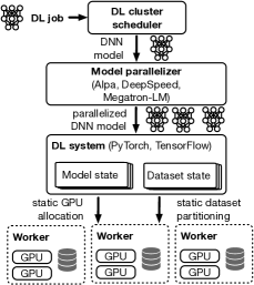
Fig. 1: Training deep learning (DL) jobs with multi-dimensional parallelism on a shared GPU cluster

Fig. 1 shows a typical deployment for training DL jobs in a shared GPU cluster. A DL cluster scheduler (e.g. Pollux [47], Gandiva [66]) manages the GPU resources and assigns jobs to GPUs. When running a job, a model parallelizer (e.g. Alpha [69], DeepSpeed [52], Megatron-LM [55]) decides on a parallelization configuration for the job by considering multiple dimensions: (1) data parallelism [29] partitions training data across workers and replicates the DNN model on all workers. Workers compute model updates using their local data partitions and synchronize these updates after each training iteration; (2) model parallelism [7] splits the model, i.e. the operators and parameters in the computational graph [1, 35, 43], and assigns partitions to different workers; and (3) pipeline parallelism [24, 37] partitions the model into stages [24]. Training data batches are then split into smaller micro-batches and pipelined across workers.

Recent advances [38, 55, 27, 16] have shown that a combination of parallelism along these dimensions, i.e. multi-dimensional parallelism, improves the performance of large DNN model training. Different parallelization configurations have different properties in terms of their scalability, device utilization, and memory consumption: data parallelism alone cannot scale to large deployments due to its synchronization overhead and large batch sizes [54]; pipeline parallelism under-utilize devices due to pipeline bubbles [37]; and model parallelism reduces the memory consumption of large models that otherwise surpass GPU memory but incurs a higher communication overhead [5]. By combining multiple strategies, model parallelizers [69, 60] navigate this trade-off space.

After generating a multi-dimensional parallelization plan, the DNN model is deployed on the GPU cluster by a DL system (e.g. PyTorch [43], TensorFlow [1], MindSpore [35]). The state of the deployed DL job consists of the dataset state and model state: the dataset state contains the partitions with the training data samples, and records the current read positions across the partitions; the model state consists of the partitioned model and optimizer parameters, and its hyper-parameters. The DL system then statically assigns the partitions of the dataset and model states to workers (see Fig. 1).

2.2 Need for dynamic resource changes

Since it may take hours, days, or weeks to run a single DL job, training e.g. a large language model (LLM) [10, 63, 39], the DL scheduler may change the GPU allocation of jobs at runtime. There are several reasons for this:

(1) Elasticity. DL schedulers may elastically increase and decrease the allocated GPUs for DL jobs based on the available resources [67, 30]. When a DL job completes, an elastic scheduler can re-allocate the freed-up GPUs to other DL jobs, e.g. giving each job a fair share of GPUs [13]. Higher priority jobs submitted to the cluster may need to take GPU resources away from already-running jobs [42].

In cloud environments [34, 15], elastic schedulers can take advantage of differences in GPU pricing. When lower cost “spot” GPUs become available [45], the scheduler may add them to existing DL jobs; when spot GPUs are preempted, jobs must continue execution with fewer GPUs. Elastic schedulers thus improve shared cluster utilization, reduce cost, and decrease completion times [65].

(2) Redeployment. DL schedulers may reallocate jobs to a new set of GPUs for operational reasons. For example, before performing hardware maintenance or upgrades, a DL job may have to be shifted to a new set of GPUs at runtime.

The redeployment of DL jobs can also reduce fragmentation in the allocated GPUs. If a job uses GPUs spread across disjoint workers, communication must use lower-bandwidth networks (e.g. Ethernet or InfiniBand) as opposed to higher-bandwidth inter-connects between GPUs (e.g. NVLink). A scheduler may therefore change the GPU allocation of a job to de-fragment it onto fewer workers [64].

(3) Failure recovery. Long-running jobs may lose GPU resources due to failures, caused by hardware faults, network outages, or software errors [10, 39]. After a fault, the job must continue execution after recovering from the last state checkpoint [36]. In some cases, the failed worker or GPUs can be replaced by new resources before resuming the job; in other cases, the job must resume with fewer GPUs, which affects its optimal parallelization configuration (see below).

2.3 Challenges when changing GPU resources

Changing the GPUs allocated to a DL job at runtime introduces several challenges:

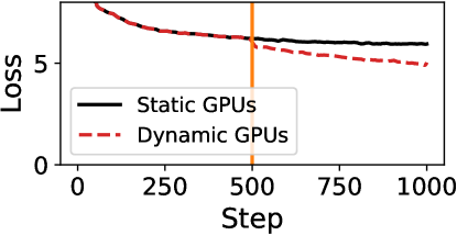
(a) Inconsistent dataset access

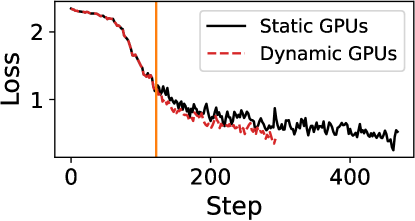
(b) Inconsistent batch size

Fig. 2: Impact of GPU change on training convergence (Changing GPUs from 2 to 4 with GPT-3 and MNIST)

(1) Impact on convergence. When changing the number of GPUs, the convergence of a DL job may be affected, and the final trained model may have e.g. a different accuracy. In today’s DL systems, job convergence depends on the specific set of GPUs used, as current jobs are not device-independent. There are multiple reasons for this:

Consistency of training dataset. A DL job must maintain dataset consistency during training, i.e. it must process training data samples exactly once and in a consistent order in each training epoch. Dataset consistency must also hold when GPU changes under data parallelism which affects the data sharding and requires re-partitioning. In particular, when re-partitioning the dataset within an epoch, the order in which data samples are ingested from that point onwards must not change.

Fig. 2(a) shows how model convergence, plotted as the loss value, is affected after adding a GPU (vertical orange line) under data parallelism. The solid black line shows regular model convergence with a static GPU allocation; the dashed red line shows convergence after the scale-out event when the dataset is processed inconsistently after re-partitioning: when resuming the training in the middle of the epoch, the first half of the training data is used twice, which overfits the model and reduces the loss value unreasonably.

Consistency of hyper-parameters. Hyper-parameter choices, such as batch sizes, and learning rate [57], depend on the GPU resources of a job. For example, the local batch size is fixed for each GPU and is typically chosen to keep devices fully utilized with data; the global batch size therefore changes with the number of GPUs.

In Fig. 2(b), we show how the global batch size must be kept constant after adding a GPU (vertical orange line) under data parallelism. The solid black line shows model convergence (measured as a loss) without the GPU change. The dashed red line shows the divergence when the GPU allocation changes but the device batch size remains unaltered.

(2) Impact on performance. The best parallelization configuration for a DL job, i.e. one achieving the lowest time-to-accuracy, depends on the GPU resources used by the job.

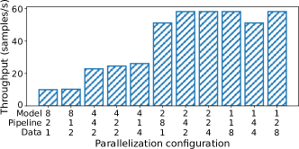
Fig. 3: Performance impact of different parallelization configurations (DL job training GPT-3 XL on 16 GPUs)

Parallelization choice. The best multi-dimensional parallelization configuration, in terms of data, model, and pipeline parallelism, depends on many factors, including the number and type of GPUs, the bandwidth and latency of the GPU inter-connect and the network between workers, and the size and structure of the DNN model architecture. Model parallelizers, e.g. Alpa [69] and Unity [60], consider these factors based on profiled performance data or analytical cost models when choosing a parallelization configuration.

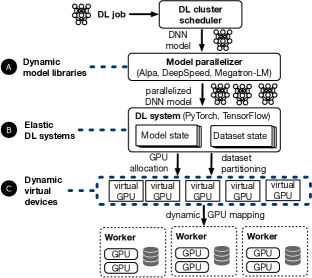
Fig. 4: Approaches for dynamic resource changes in DL jobs

	Approach	Systems	Consistency		Parallelism						Reconfiguration
			Dataset	Hyper-params	Static			Dynamic			overhead
					DP	PP	MP	DP	PP	MP
	Model libraries	Alpa [69]	-	-	✓	✓	✓	-	-	-	-
		Megatron-LM [55]	-	-	✓	✓	✓	✓	✗	✗	full state
		Deepspeed [52]	✓	✓	✓	✓	✗	✓	✗	✗	full state
	Elastic DL systems	Elastic Horovod [23]	✗	✗	✓	-	-	✓	-	-	full state
		Torch Distributed [46]	✓	✗	✓	✓	(✓)	✓	(✓)	(✓)	full state
		Varuna [4]	✓	✓	✓	✓	-	✓	✓	-	full state
		KungFu [33]	✓	✓	✓	-	-	✓	-	-	full state
	Virtual devices	VirtualFlow [41]	✓	✓	✓	-	-	✓	-	-	full state
		EasyScale [31]	✓	✓	✓	-	-	✓	-	-	full state
		Singularity [56]	✓	✓	✓	✓	✓	✓	✗	✗	GPU state
State management		Tenplex	✓	✓	✓	✓	✓	✓	✓	✓	minimal state

Table 1: Comparison of existing proposals for supporting dynamic GPU changes in DL jobs

When the GPU resources of a DL job change at runtime, a parallelization configuration that was optimal at deployment time may no longer be optimal with the new resources. We demonstrate this empirically in Fig. 3, which shows the training throughput (in samples/second) when training the GPT-3 XL [6] model using Megatron-LM [55] on 16 GPUs under a range of parallelization configurations. Each parallelization configuration varies the degree of data ($D$), model ($M$), and pipeline ($P$) parallelism, and thus alters the GPU allocation.

As the results show, the training throughput differs by over 5$\times$ between the best and the worst configuration, despite the fact that each configuration uses the same number of GPUs (16). The configuration $(M,P,D)=(2,4,2)$ performs well because constrains communication-intensive model parallelism within workers; in contrast, the configuration $(8,2,1)$ performs the worst because model parallelism must use the slower inter-worker links.

Reconfiguration cost. Changing the parallelization of a DL job means that the partitioned dataset and model state are no longer correct. The state must be re-partitioned and the new dataset and model partitions must be made available to the workers. This involves large amounts of data movement, which results in a performance overhead. For example, prior industry work [56] reports that reducing the GPU allocation for a DL job from 16 to 8 GPUs may take 122 secs.

2.4 Current approaches

A number of approaches have been proposed to allow DL schedulers to change GPU resources dynamically. We give an overview, and then discuss specific proposals, assessing them against the challenges from §2.3.

Fig. 4 shows the main three approaches:  dynamic model libraries adapt to changes in GPUs by producing a new parallelization configuration at runtime;  elastic DL systems include support to scale GPU resources out and in at runtime; and  virtual devices decouple physical GPUs from logical GPUs that are exposed to the DL systems, allowing the mapping to change at runtime.

Tab. 1 compares systems that implement these approaches:

Model libraries. The Alpa model parallelizer [69] only provides a parallelization configuration at job deployment time and does not support dynamic changes. Megatron-LM [55] and DeepSpeed [52] support dynamic resource changes under data parallelism only by dividing batches into micro-batches [58, 50]. By changing the allocation of micro-batches only, DeepSpeed ensures consistency after resource changes. Since the full training state is moved to and from remote storage, there is a substantial reconfiguration overhead.

In summary, model libraries with support for dynamic reconfiguration are limited in terms of support for multi-dimensional parallelism, and they lack integration with DL systems, which requires manual state re-partitioning.

Elastic DL systems enable training with dynamic resource changes. Elastic Horovod [53] exposes the model state through a user-defined state object. It allows users to synchronize state across workers when changing data parallelism, but any state re-distribution must be implemented consistently by users. In particular, the dataset state can become inconsistent if scaling does not occur at epoch boundaries. Torch Distributed Elastic/Checkpoint [32] provides a model broadcast API to save/resume model checkpoints and allows users to implement re-partitioning operations using a distributed tensor abstraction. Users must ensure the consistency of hyper-parameters and perform the required data movement between workers. Varuna [4] lets the user define cut-points at which the model pipeline is partitioned at runtime when resources change. KungFu [33] uses a broadcast operation to distribute the training state and with it the model replicas.

Overall, elasticity support in DL systems either does not account for full multi-dimensional parallelism or requires users to implement state re-partitioning and distribution manually.

\begin{overpic}[width=216.81pt]{figures/overview} \put(-2.0,21.0){\scalebox{0.78}{ \leavevmode\hbox to9.93pt{\vbox to9.93pt{\text{[drawing]}}}}} \put(40.0,55.0){\scalebox{0.78}{ \leavevmode\hbox to9.93pt{\vbox to9.93pt{\text{[drawing]}}}}} \put(-2.0,40.0){\scalebox{0.78}{ \leavevmode\hbox to9.93pt{\vbox to9.93pt{\text{[drawing]}}}}} \put(49.5,34.0){\scalebox{0.78}{ \leavevmode\hbox to9.93pt{\vbox to9.93pt{\text{[drawing]}}}}} \put(49.5,14.0){\scalebox{0.78}{ \leavevmode\hbox to9.93pt{\vbox to9.93pt{\text{[drawing]}}}}} \end{overpic}

Fig. 5: Tenplex design

Virtual devices make DL jobs device-independent by virtualizing resources and allowing the mapping between virtual/physical resources to change at runtime. The set of virtual resources exposed to a job represents the maximum number of physical resources available at runtime.

VirtualFlow [41] uses an all-gather operation to send the current training state to the new workers. To ensure dataset consistency, it follows exactly once semantics for data loading. The same is true for EasyScale [31], which adopts a thread abstraction and performs process snapshotting to capture the state. Singularity [56] obtains the full GPU state through GPU virtualization at the CUDA driver level.

As a consequence, virtual device approaches are effective at supporting dynamic data parallelism, which does not require re-partitioning, but they cannot support runtime changes under general multi-dimensional parallelism.

3 Tenplex Design

As Tab. 1 shows, the goal of Tenplex is to create an approach for supporting dynamic resource changes of DL jobs that maintains (i) the consistency of the training result, (ii) supports arbitrary reconfiguration under multi-dimensional parallelism, and (iii) ensures a low reconfiguration overhead. We base our approach on the observation that dynamic resource changes at runtime affect the state of a DL job but existing DL systems lack an abstraction to expose the DL job state and transform it, as required.

Fig. 5 shows the basic idea behind Tenplex, a statement management library for DL systems that enables dynamic resource change. Tenplex externalises the DL job state (see  ), representing it as a parallelizable tensor collection (PTC). A PTC provides a hierarchical tensor representation of the model and dataset set of the job, and it enables Tenplex to map the state to GPU devices under a given parallelization configuration.

Tenplex integrates with a DL cluster scheduler. When the scheduler makes a decision to change the GPU allocation of a job at runtime by increasing or decreasing it, it notifies Tenplex ( ). Tenplex then uses its State Transformer ( ) to obtain a new parallelization configuration for the job that reflects the change resource allocation from a model parallelizer, such as Alpa [69] or Megatron-LM [55] ( ). Based on the new parallelization configuration, the State Transform then calculates a reconfiguration plan, which describes how the state represented by the PTC must change across the cluster to implement the new configuration. The reconfiguration is then implemented as part of the cluster by repartitioning and redistributing the data and model state ( ).

Next, §4 describes how a PTC is defined, expresses multi-dimensional parallelism, and can be used to obtain a reconfiguration plan after a resource change. §5 explains how Tenplex interfaces with the DL system and how it implements the state changes required by the reconfiguration plan efficiently.

4 Parallelizable Tensor Collection

Next, we define a ${\mathop{\mathrm{PTC}}}$ (§4.1), explain how it expresses different parallelizations (§4.2), and can be used to generate reconfiguration plans (§4.3).

4.1 Definition

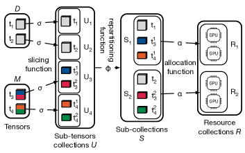
Fig. 6: PTC collection and functions mapping

A ${\mathop{\mathrm{PTC}}}$ represents the execution state of a DL job: it includes the dataset state that contains the training data and an iterator that records processed training data in the current epoch and the model state that constitutes of the DNN model parameters of all layers. A ${\mathop{\mathrm{PTC}}}$ expresses both types of state in a unified manner as a collection of tensors, which Tenplex re-partitions when changing the parallelization configuration.

The parallelization configuration of the DL job, i.e. how the dataset and model states are partitioned under multi-dimensional parallelism, is expressed as three functions: for model parallelism, a slicing function splits tensors into sub-tensors; for data and pipeline parallelism, a partitioning function partitions the sub-tensors into sub-collections; and an allocation function describes the mapping of sub-collections to devices, thus representing parallel execution of a DL job. Tenplex obtains the parallelization configuration, in terms of the slicing, partitioning, and allocation functions, from a model parallelization library (e.g. Megatron-LM [55]) or a model parallelizer (e.g. Alpha [69], Unity [60]). When the functions change at runtime due to a resource change, Tenplex transforms the state modeled by the ${\mathop{\mathrm{PTC}}}$ accordingly to adapt DL job execution.

Formally, we define the ${\mathop{\mathrm{PTC}}}$ as a tuple of a model tensor collection $M$, a dataset tensor collection $D$, a slicing function $\sigma$, a partitioning function $\phi$, and an allocation function $\alpha$:

$${\mathop{\mathrm{PTC}}}=(M,D,\sigma,\phi,\alpha)$$ (1)

where $M$ and $D$ are sets of tensors for model parameters and dataset samples, $M=\{t_{1},\dots,t_{n}\}$, $D=\{t_{n+1},\dots,t_{n+m}\}$; $\sigma$ slices a tensor $t$ into sub-tensors, $\sigma(t)=\{t^{1},..,t^{n}\},t\in M\cup D$. We denote all sets of sub-tensors as $U$, i.e. $U=\{\sigma(t_{1})\dots\sigma(t_{n+m})\}$; $\phi$ partitions $U$ into sub-collections, $\phi(U)=\{S_{1},..,S_{p}\}$; $\alpha$ allocates sub-collections to devices of the resource pool $R$, $\alpha(S_{i})=\{r_{1},..,r_{q}\}$.

We illustrate the PTC definition with the following example:

PTC example. In Fig. 6, the slicing function $\sigma$ slices each tensor in the dataset $D=\{t_{1},t_{2}\}$ and the model $M=\{t_{3},t_{4}\}$, and creates the sub-tensor set $U$, $\sigma(t_{3})=U_{3}=\{t_{3}^{1},t_{3}^{2}\}$; the partitioning function $\phi$ takes $U$ and groups it into sub-collections $S$; the allocation function $\alpha$ assigns each sub-collection $S_{i}$ a resource set $R_{i}$, e.g. the sub-collection $S_{2}$ with $t_{4}^{2}$ is assigned to resources $R_{2}$.

4.2 Parallelizations

Next, we show how a PTC represents multi-dimensional parallelization configurations (i.e. data, model, and pipeline parallelism) by using different slicing functions $\sigma$, partitioning functions $\phi$, and allocation functions $\alpha$. We assume a $n$-parameter model, $M=(t_{1},\dots,t_{n})$, a $m$-sample dataset, $D=(t_{n+1},\dots,t_{n+m})$, and $k$ GPU devices, $R=(r_{1},\dots,r_{k})$:

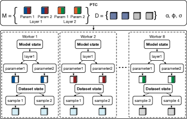
Fig. 7: PTC with multi-dimensional parallelism on 8 GPUs

Data parallelism (DP) replicates the model and partitions the data samples across $k$ GPUs. This means that $M$ and $D$ are not sliced, $\sigma(t)=\{t\},\forall t\in M\cup D$ and $U=\{\{t_{1}\},\dots,\{t_{n+m}\}\}$. The partitioning function $\phi$ groups the model together as one sub-collection, and each data partition as a sub-collection, $\phi(U)=\{S_{1},\dots,S_{k+1}\}$, where $S_{1}=M$ and $S_{2}$ to $S_{k+1}$ are the data sub-collections.

Finally, the allocation function $\alpha$ assigns the model sub-collections to all $k$ GPUs, $\alpha(S_{1})=\{r_{1},\dots,r_{k}\}$. It assigns the data sub-collections across $k$ GPUs, $\alpha(S_{i+1})=\{r_{i}\},\forall S_{i}\in S,1\leq i\leq k$. In practice, a DL job trains models on data batches, therefore, $\phi$ and $\alpha$ are applied to each batch.

Model parallelism (MP) slices each tensor of model parameters into $k$ sub-tensors, $\sigma(t)=\{t^{1},\dots,t^{k}\},\forall t\in M$. In contrast, the dataset $D$ is not sliced, $\sigma(t)=\{t\},\forall t\in D$. The sub-tensor collection is $U=\{\{t_{1}^{1},\dots,t_{1}^{k}\},\dots,\{t_{n}^{1},\dots,t_{n}^{k}\},\{t_{n+1}\},\dots\{t_{n+m}\}\}$.

The partitioning function $\phi$ then groups the sub-tensors to $k+1$ sub-collections, $\phi(U)=\{S_{1},\dots,S_{k+1}\}$, while ensuring a sub-collection has one sub-tensor of each parameter, $S_{i}=\{t_{1}^{i}\dots t_{n}^{i}\},1\leq i\leq k$. The dataset tensors form $S_{k+1}$. The allocation function $\alpha$ assigns each model sub-collection to a GPU, $\alpha(S_{i})=\{r_{i}\},1\leq i\leq k$, while distributing the whole dataset to all GPU devices, $\alpha(S_{k+1})=\{r_{1},\dots,r_{k}\}$.

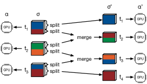
Fig. 8: Example of a reconfiguration plan

Pipeline parallelism (PP) partitions sets of layers and allocates them across $k$ GPUs. It does not slice model tensors nor the dataset, $\sigma(t)=\{t\},\forall t\in D\cup M$, but partitions these tensors into $k$ sets of layers, $\phi(U)=\{S_{1},\dots,S_{k+1}\}$.

The partitioning function is defined in the parallelization configuration. Without loss of generality, we assume that layers are evenly partitioned, and each layer has the same number of parameters: $\phi$ maps $t_{i}$ to $S_{j}$ where $j=\lfloor\frac{i}{\lceil n/k\rceil}\rfloor$. $S_{k+1}=D$ for the dataset. Data samples are only needed at the first layer as the input and the last layer to compute the loss value, $\alpha(S_{k+1})=\{r_{1},r_{k}\}$. The model sub-collections are allocated to one GPU, $\alpha(S_{i})=\{r_{i}\},1\leq i\leq k$.

Multi-dimensional parallelism (MDP) combines the above strategies. Fig. 7 shows a sample PTC that slices, partitions, and allocates $M=\{t_{1},t_{2},t_{3},t_{4}\}$ and $D=\{t_{5},t_{6},t_{7},t_{8}\}$ to 8 GPUs with a parallelism of $2$ in each dimension: for MP of degree 2, $\sigma$ slices each parameter tensor into two sub-tensors, i.e. $\forall t\in M,\sigma(t)=\{t^{1},t^{2}\}$. No slicing occurs for the dataset, $U=\{\{t_{1}^{1},t_{1}^{2}\},\dots,\{t_{4}^{1},t_{4}^{2}\},\{t_{5}\},\dots\{t_{8}\}\}$; for MP and PP of degree 2, $\phi$ partitions the sub-tensor collections $U$ into 4 sub-collections, $S_{1}=\{t_{1}^{1},t_{2}^{1}\}$, $S_{2}=\{t_{1}^{2},t_{2}^{2}\}$, $S_{3}=\{t_{3}^{1},t_{4}^{1}\}$, and $S_{4}=\{t_{3}^{2},t_{4}^{2}\}$; for DP of degree 2, there are an extra 2 sub-collections, $S_{5}=\{t_{4},t_{5}\}$ and $S_{6}=\{t_{6},t_{7}\}$.

The allocation function $\alpha$ assigns each model sub-collection to 2 GPUs due to model replication of DP, i.e. $\alpha(S_{i})=\{r_{i},r_{i+4}\},1\leq i\leq 4$, while $\alpha$ allocates each data sub-collection to GPUs consisting of one model replica, i.e. $\alpha(S_{5})=\{r_{1},\dots,r_{4}\}$ and $\alpha(S_{6})=\{r_{4},\dots,r_{8}\}$.

Data: ${\mathop{\mathrm{PTC}}}=(M,D,\sigma,\phi,\alpha)$

${\mathop{\mathrm{PTC}}}^{\prime}=(M,D,\sigma^{\prime},\phi^{\prime},\alpha^{\prime})$

Result: $\mathcal{P}$: Reconfiguration Plan

1

2$U\leftarrow\emptyset$, $U^{\prime}\leftarrow\emptyset$

3 foreach $t\in M\cup D$ do // iterate all tensors

4       $U_{t}\leftarrow\sigma(t)$, $U^{\prime}_{t}\leftarrow\sigma^{\prime}(t)$

5       if $U_{t}\neq U^{\prime}_{t}$ then // sub-tensor collections differ

6             $\mathcal{P}\leftarrow\mathcal{P}\cup\textrm{reslice}(U_{t},U^{\prime}_{t})$ // add re-slice operation

7            

8      $U\leftarrow U\cup U_{t}$, $U^{\prime}\leftarrow U^{\prime}\cup U^{\prime}_{t}$

9      

10$S\leftarrow\phi(U)$, $S^{\prime}\leftarrow\phi^{\prime}(U^{\prime})$ // partition sub-tensor collections

11 foreach $S^{\prime}_{i}\in S^{\prime}$ do

12       if $\textrm{find-equal-sub-collection}(S^{\prime}_{i},S)$ then // sub-collection exists

13             $R_{i}\leftarrow\alpha(S^{\prime}_{i})$, $R^{\prime}_{i}\leftarrow\alpha^{\prime}(S^{\prime}_{i})$

14             if $R_{i}\neq R^{\prime}_{i}$ then // resources differ

15                   $\mathcal{P}\leftarrow\mathcal{P}\cup\textrm{reallocate}(S_{e},R^{\prime}_{i})$

16                  

17      else  // sub-collection does not already exist

18             $\mathcal{P}\leftarrow\mathcal{P}\cup\textrm{repartition}(S^{\prime}_{i})$

19             $\mathcal{P}\leftarrow\mathcal{P}\cup\textrm{reallocate}(S^{\prime}_{i},R^{\prime})$

20            

21func reslice($U_{t}$: Sub-Tensor-Collection, $U^{\prime}_{t}$: Sub-Tensor-Collection)

22       $B\leftarrow\textrm{infer-boundaries}(U_{t})$, $B^{\prime}\leftarrow\textrm{infer-boundaries}(U^{\prime}_{t})$

23       $L\leftarrow\emptyset$

24       foreach $b^{\prime}\in B^{\prime}$ do // check every boundary

25             if $b^{\prime}\notin B$ then // not already split at boundary

26                   $L\leftarrow L\cup\textrm{split}(U_{t},b^{\prime})$

27                  

28      $\textrm{merge}(L,B^{\prime})$

29      

Algorithm 1 Reconfiguration algorithm

4.3 Reconfiguration plan

A ${\mathop{\mathrm{PTC}}}$ captures the DL job state on a given set of GPU resources $R$. When the GPU allocation changes, Tenplex creates a new ${\mathop{\mathrm{PTC}}}^{\prime}$. Tenplex must then transform the job state from the previous configuration to the new one. A reconfiguration plan describes how to transform the job state with minimal data movement between workers and GPUs.

To generate a reconfiguration plan, Tenplex considers the differences between previous functions ($\sigma$, $\phi$, and $\alpha$) and the new functions ($\sigma^{\prime}$, $\phi^{\prime}$, and $\alpha^{\prime}$): It generates a sequence of re-slice, re-partition or re-allocate operations for the ${\mathop{\mathrm{PTC}}}$.

Reconfiguration operations. (i) re-slice: if the sub-tensor collections $U$ of ${\mathop{\mathrm{PTC}}}$ and $U^{\prime}$ of ${\mathop{\mathrm{PTC}}}^{\prime}$ are different, re-slice first slices the previous sub-tensors and then merges them according to the dimensions specified in the parallelization configuration. (ii) re-partition: if any parts of sub-collections $S^{\prime}$ of ${\mathop{\mathrm{PTC}}}^{\prime}$ do not exist in the previous $S$ of ${\mathop{\mathrm{PTC}}}$, re-partition creates these new sub-collections. (ii) re-allocation: if a sub-collection changes its resources, $\alpha(S_{i})\neq\alpha^{\prime}(S_{i})$, re-allocation moves elements of sub-collection from the previous resources $R_{i}$ to the new resources $R^{\prime}_{i}$ (i.e. different GPUs).

Example. Fig. 8 shows a reconfiguration plan. Here, the previous ${\mathop{\mathrm{PTC}}}$ has MP of degree 3, $\sigma(t)=\{t_{1},t_{2},t_{3}\}$, and allocated to 3 GPUs. In contrast, the new ${\mathop{\mathrm{PTC}}}^{\prime}$ has MP of degree 4, which requires the tensor $t$ sliced into 4, $\sigma^{\prime}(t)=\{t_{1},t_{2},t_{3},t_{4}\}$. Based on the new sub-tensor shapes and the previous slicing $\sigma$, Tenplex infers the slicing and merging dimensions/positions of the tensor $t$. The new sub-tensors $t_{1}$ and $t_{4}$ do not need merging, but, for $t_{2}$ and $t_{3}$, the split sub-tensors are merged.

Reconfiguration plan. Alg. 1 formalizes the reconfiguration plan $\mathcal{P}$ based on ${\mathop{\mathrm{PTC}}}$ and ${\mathop{\mathrm{PTC}}}^{\prime}$. First, it iterates over all tensors of $M$ and $D$ (line 1), applying slicing functions $\sigma$ and $\sigma^{\prime}$ to the tensor $t$ (line 1). If the sub-tensor collections are different, a re-slice is added (lines 1–1). The reslice function (lines 1–1) infers the re-slicing dimensions and boundaries. If a tensor is not split at the new boundary $B^{\prime}$, the sub-tensor is split at the boundary $b^{\prime}$. The merge function combines the split sub-tensors and removes the parts of previous tenors according to boundaries $B$.

After adding re-slicing operations, it iterates over all new sub-collections $S^{\prime}$. If a new sub-collection $S^{\prime}_{i}$ is already in the previous one $S$ and the resources $R_{i}$ and $R^{\prime}_{i}$ are different, a re-allocate is added to $\mathcal{P}$ (lines 1–1); otherwise, re-partition and re-allocate are added (lines 1–1).

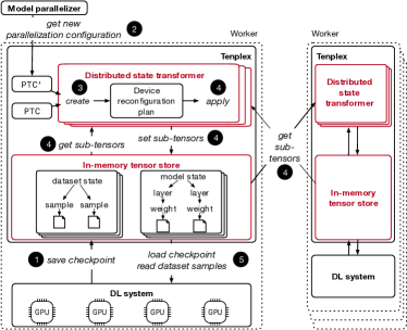
Fig. 9: Tenplex architecture

5 Tenplex Architecture

In this section, we describe the architecture of the Tenplex state management library that uses PTCs to adapt DL jobs based on resource changes.

5.1 Overview

Fig. 9 shows the Tenplex architecture. Tenplex executes on each worker and has two main components, a distributed state transformer and an in-memory tensor store: the state transformer inputs the model and dataset partitions from a previous ${\mathop{\mathrm{PTC}}}$ and creates new partitions to comply with a new ${\mathop{\mathrm{PTC}}}^{\prime}$ after a resource change; the tensor store maintains the model and dataset state partitions represented by the PTC in a hierarchical virtual in-memory file system.

5.2 State transformer

Each time the resources of a DL job change, Tenplex must create a new model and dataset state partitions for the DL system to continue executing the job. Since these state transformations can be parallelized, Tenplex maintains an instance of the state transformer for each resource $r$ on a worker. Each transformer instance applies the reconfiguration plan.

As Fig. 9 shows, the state transformer modifies the DL job after notification from the job scheduler of a resource change:

Tenplex obtains the training state from the DL system by getting a model checkpoint per GPU. Each checkpoint is written to a model state partition in the tensor store.  Tenplex then requests a new parallelization configuration from the model parallelizer. The new configuration is expressed as ${\mathop{\mathrm{PTC}}}^{\prime}$ and becomes the basis for the reconfiguration.  Each state transformer instance uses Alg. 1 to create the device’s reconfiguration plan. It compares ${\mathop{\mathrm{PTC}}}$ and ${\mathop{\mathrm{PTC}}}^{\prime}$ and infers the transformation operations.  The state transformer then applies the reconfiguration plan in terms of re-slice, re-partition, and re-allocation operations to generate the new training state partitions (see §4.3). It requests the necessary sub-tenors for the worker by retrieving them either from the local or remote tensor stores and saves them in the local tensor store.  Finally, it instructs the DL system to restore from per-GPU checkpoints based on the transformed model partitions in the local tensor store. After restarting the job, the DL system continues reading data samples from the local tensor store.

The model parallelizer provides the parallelization configuration to Tenplex as a JSON object, with the values being tensor shapes. The object structure must match the model checkpoint. In contrast to checkpoints, tensors are replaced with metadata. Since the job is distributed, each GPU requires its own JSON object with a parallelization configuration.

5.3 Tensor store

Each worker has an in-memory tensor store that holds the model and dataset partitions for each local GPU. The tensor store maintains the model and dataset tensors in a hierarchical in-memory file system. The hierarchy follows the model structure, with parameters represented as leaves.

API. The tensor store exposes APIs to the state transformer to apply a reconfiguration plan, and to the DL system to load/store the model state. It supports a NumPy-like [19] array interface for requesting tensors through a REST API: a /query request with a path attribute obtains a tensor; an upload request adds a new tensor to the store at a path.

A unique feature of the interface is that it can be used to request sub-tensors, by defining a range for a dimension, similar to a Python slice. Requesting sub-tensors is important to perform the required re-slicing under model parallelism. To reduce data movement between workers, the state transformer requests sub-tensors instead of complete tensors that must be split after transfer. To get a sub-tensor, the query includes a range attribute whose values specify the dimension and range. For example, a query for the second dimension is range=:,2:4, which returns the sub-tensor for $[2,4)$.

Tenplex also gives a simple API to the DL system to move the model state in and out of the tensor store. To save the model state, tenplex.save(model, path) maps a Python dictionary to the virtual file system and sets each tensor with a request; tenplex.load(path) maps the virtual file system tree back to a Python dictionary.

State representation. The model state in the tensor store is represented as a tree with nodes grouping parameters. For example, /2/embedding/weight is the weight parameter of the embedding layer for model state partition $2$. The leaves are sub-tensors, which are implemented as NumPy arrays to give compatibility with most DL systems.

The training dataset consists of binary files with data samples. An index file holds the byte offsets for each data sample, the number of binary files, the paths to the binary files, and the number of data samples. While the binary representation could be any format, samples are tensors and therefore Tenplex uses NumPy [19] (npy or npz) arrays. Based on the index file, the state transformer can repartition the dataset if the data parallelism changes.

To read data sample $i$, a DL job reads byte range $i$ in the index file and then reads the corresponding part of the binary file storing the data sample. Before training starts, the DL job adds the dataset by pointing Tenplex to the index file. Tenplex fetches the dataset partitions into the tensor stores.

In contrast to the model state, the training dataset is immutable and consumed sequentially. Tenplex leverages this to improve performance: it caches the dataset in a data sample buffer on the workers and streams the samples.

Typically, especially in cloud settings, the training dataset is stored on remote storage, such as S3 [3] or other blob storage [34, 15]. Tenplex maintains a lookup table to track the location of data samples. It distinguishes whether data samples are remote or available in the local data sample buffer on the worker. Since the interconnect between workers is usually faster than access to remote storage, Tenplex prioritizes fetching samples from other workers. It can overlap training and dataset fetching because the complete dataset does not need to be available when a DL job starts.

5.4 Fault tolerance

When workers or GPUs fail during job execution, Tenplex relies on the DL systems’ checkpointing mechanism for fault tolerance. When a failure occurs, the job state is recovered from the persisted checkpoints.

Consequently, there is the usual trade-off between checkpointing frequency and overhead. With infrequent checkpointing, some of the job progress is lost. For DL jobs with data parallelism, Tenplex compensates for this by exploiting that the model state is replicated among workers. As long as one model replica still exists after a failure, the state can be obtained from that GPU. Tenplex exploits this to avoid re-executing training steps due to stale checkpoints.

To lower the cost of recovery from high-frequent failures, Tenplex can replicate its model state in the tensor store across workers in a round-robin fashion. Based on the number of replicas $n$, the state is replicated to the next $n$ workers. Since a failure can be seen as a resource reduction, the state transformation of Tenplex helps mitigate the failure, without having to wait for alternative resources to become available.

6 Evaluation

In this section, we first evaluates Tenplex in three use cases: supporting the elastic scaling of multi-dimensional parallelism, enabling job redeployment, and handling failure recovery. After that, we explore the scalability of Tenplex. Finally, we assess the impact of Tenplex on both the performance and model convergence when supporting the change of parallelism configurations.

6.1 Experimental setup

Our experiments have the following setup:

Cluster. We conduct on-premise experiments with 4 machines with 4 GPUs each, giving a total of up to 16 GPUs. Each machine has an AMD EPYC 7402P CPU, 4 NVIDIA RTX A6000 GPUs, and are interconnected with 100-Gbps InfiniBand. The GPUs are interconnected with third-generation NVLink and PCIe 4.0. We also conduct large-scale cloud experiments on Azure [34] with Standard_NC24s_v3 virtual machines, which have 4 NVIDIA V100 GPUs each.

Baselines. We compare Tenplex to multiple baselines: (i) DeepSpeed v0.6 [52] in combination with Megatron-LM v2.4, which represents the model library approach. It can only scale along the data parallelism dimension; (ii) Horovod-Elastic v0.28 [23], which is a state-of-the-art elastic DL system that also only supports data parallelism; and (iii) Singularity that follows the virtual devices approach. Since Singularity is not open-source, we report results from the paper [56].

Models. We use these DNN models: (i) BERT-large with 340 million parameters; (ii) GPT-3 with 1.3 B (XL), 2.7 B, and 6.7 B parameters; and (iii) ResNet50 with 25 M parameters.

Datasets. For the training data, we use: (i) OpenWebText [14] with 2 M samples with a sequence length of 1024; (ii) Wikipedia [12] with 6.8 M samples with the same sequence length; and (iii) ImageNet [8] with 1 M samples.

6.2 Elastic multi-dimensional parallelism

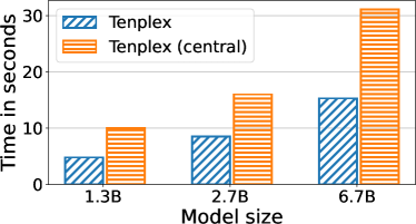
Fig. 10: Redeployment time of DL job

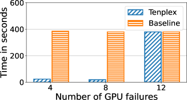
Fig. 11: Failure recovery time (GPT-3 2.7 B)

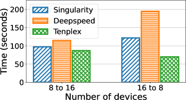
Fig. 12: Reconfiguration time

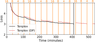
Fig. 13: Convergence of elastic DL job with multi-dimensional parallelism under dynamic GPU changes

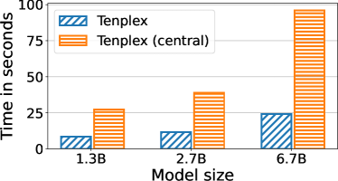
(a) Data parallelism

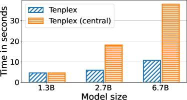
(b) Pipeline parallelism

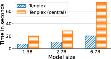
(c) Model parallelism

Fig. 14: Reconfiguration time with different parallelizations

We evaluate the benefits of supporting elasticity in DL jobs with multi-dimensional parallelism, scaling across all parallelism dimensions when the GPU allocation changes.

The experiment uses the GPT-3 XL model on the on-premise cluster. The DL job runtimes and associated scaling events were modelled based on Microsoft’s Philly trace [26]: over the runtime of 538 mins, we scale on average every 35 mins. During a scaling event, we change the number of GPUs for a job between 16, 8, and 4 GPUs.

We compare the training convergence of Tenplex to Tenplex (DP only), which is similar to DeepSpeed or Megatron-LM with PyTorch Elastic in that it can execute a job with multi-dimensional parallelism but only scale it dynamically along the DP dimension. In contrast, Tenplex scales from $(M,P,D)=(2,4,2)$ to $(2,2,2)$ to $(2,1,2)$, which are the parallelization configurations that achieve the best performance. Tenplex (DP only) scales $(M,D,P)=(2,4,2)$ to $(2,4,1)$, and pauses training with $4$ GPUs because a configuration with a PP of $4$ and MP of $2$ cannot run with $4$ GPUs.

Fig. 13 shows the loss over time, and the scaling events are indicated as vertical orange lines, annotated by the GPU count. As we can see, it takes Tenplex only 409 mins to reach the same loss that Tenplex (DP only) only reaches after 538 mins—a reduction by 24%. Since Tenplex can support scaling along all dimensions, it exploits more optimal parallelization configurations—using resources more effectively.

6.3 Job redeployment

We evaluate how long the redeployment of DL jobs with different model sizes using Tenplex takes for different GPU resources. We compare to a baseline approach for dynamic job redeployment in which all state is held at a single central storage location. The goal is to evaluate the benefit of Tenplex’s distributed state management design.

In the experiment, we redeploy a DL job with multi-dimensional parallelism from a set of 8 GPUs to another set of 8 GPUs. We measure the redeployment time on the on-premise clyster with the GPT-3 model with sizes of 1.3 B, 2.7 B, and 6.7 B. The parallelization configuration is $(M,D,P)=(4,2,1)$ and remains the same, as the number of GPUs is constant. We compare to Tenplex (central), which saves all training state at a single worker, following the approach of PyTorch Elastic [46] or DeepSpeed [52].

Fig. 12 shows the redeployment time under different model sizes. Tenplex achieves a lower redeployment time than Tenplex (central) for all model sizes: the time for the central approach is 2.1$\times$ for the 1.3 B size, 1.9$\times$ for 2.7 B size, and 2$\times$ for 6.7 B size, respectively, higher compared to Tenplex. Since Tenplex’s distributed state management migrates state directly between workers, it avoids a single worker becoming a bottleneck that would increase redeployment time.

6.4 Failure recovery

We explore how Tenplex handles dynamic resource scenarios that require reconfiguration due to failures. We emulate faults of 4, 8, and 12 GPUs and measure failure recovery times. We use the GPT-3 2.7 B model with the Wikipedia dataset, running on the on-premise cluster. We compare Tenplex to a baseline, which always recovers from the last checkpoint. We assume an average loss of 50 training steps. The parallelization configuration is $(M,P,D)=(4,2,2)$, i.e. there is one replica of the model.

Fig. 12 shows that recovery time (in seconds) with different numbers of failed GPUs. Tenplex recovers faster than the baseline if there exists at least one model replica, e.g. for failures with 4 and 8 GPUs. Here, Tenplex does not need to rerun the lost training steps, because it does not rely on the stale checkpointed state for recovery. With $8$ GPUs Tenplex takes only $5$% of the recovery time of the baseline, which exhibits the same cost as for 12 GPUs. When there are no model replicas available, Tenplex uses the last checkpoint and only achieves a slight performance benefit due to using local instead of remote storage. We conclude that Tenplex reduces failure recovery times if model replicas are available as part of the parallelization configuration.

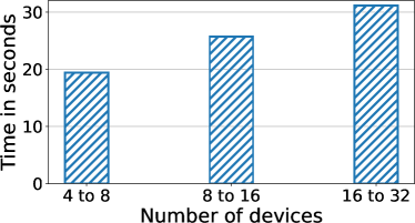
(a) Data parallelism

(b) Pipeline parallelism

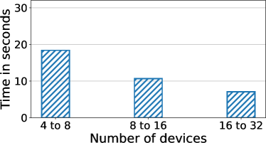
(c) Model parallelism

Fig. 15: Reconfiguration time with different cluster sizes (GPT-3 XL 1.3 B)

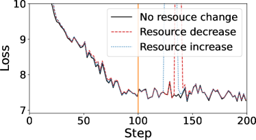
(a) Data parallelism

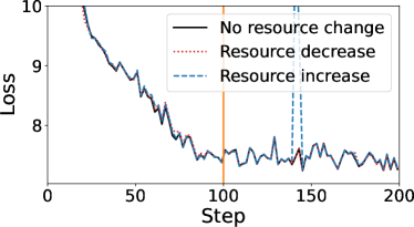
(b) Pipeline parallelism

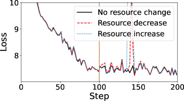
(c) Model parallelism

Fig. 16: Model convergence with reconfiguration

6.5 Different reconfiguration approaches

The experiment compares (i) our state management approach (Tenplex) with (ii) a virtual device approach that performs full GPU state migration (Singularity) and (iii) a model library of an elastic DL system (DeepSpeed).

We use the GPT-3 XL model with the Wikipedia dataset on the on-premise cluster. We perform one experiment that scales down resources from 16 to 8 GPUs and another that scales up from 8 to 16 GPUs. Since Singularity is closed-source, we report the paper figures on similar hardware [56].

Fig. 12 shows the reconfiguration time (in seconds). When changing from 8 to 16 GPUs, Tenplex requires 24% less time than DeepSpeed and 10% less time than Singularity. The difference becomes larger when scaling from 16 to 8 GPUs: Tenplex needs 64% less time than DeepSpeed and 43% less than Singularity. Singularity is slower, because, besides the training state, it also moves the full GPU device state. DeepSpeed suffers from the fact that it does not include graceful mechanisms for informing DeepSpeed about reconfiguration, but uses its failure detection mechanism. The state management approach of Tenplex is the fastest, as it is aware of data locality and minimizes state movement.

6.6 Impact of model size

Next, we examine the impact of model size on reconfiguration time when changing parallelization configuration. We deploy Tenplex and Tenplex (central), which manage the state in a single node, with the different GPT-3 models on the on-premise cluster. For data parallelism (DP), we change the configuration from $(M,P,D)=(4,2,1)$ to $(4,2,2)$; for pipeline parallelism (PP) from $(4,2,1)$ to $(4,4,1)$; and for model parallelism (MP) from $(4,2,1)$ to $(8,2,1)$.

Fig. 14 shows the reconfiguration time (in seconds) for different model sizes and parallelisms. Under DP (Fig. 14(a)), Tenplex (central) with GPT-3 6.7 B takes 4$\times$ longer than Tenplex, because of the limited network bandwidth of a single worker in comparison with a distributed peer-to-peer state reconfiguration. We observe the same behavior for PP and MP: for PP (Fig. 14(b)), the centralized version takes 3.5$\times$ longer and, for MP (Fig. 14(c)), it takes 3.7$\times$ longer. The only exception is PP with 1.3 B parameters, because the network bottleneck is not reached, and it does not involve splitting/merging sub-tensors. The centralized approach becomes a bottleneck, especially with many model parameters, due to the limited network bandwidth and less parallelism of the state transformation on a single worker.

6.7 Impact of resource count

Next, we keep the model size fixed but change the GPU resources in the cluster to explore how the cluster size and parallelization configuration impact the reconfiguration time.

The model is GPT-3 XL with the Wikipedia dataset deployed in the cloud testbed. We scale the resources from 4 to 8, 8 to 16, and 16 to 32 GPUs for data, model, and pipeline parallelism, respectively. For each parallelization configuration, if the number of GPUs doubles, the degree of parallelism also doubles. We compare Tenplex with the baseline Tenplex (central), as before.

Fig. 15 shows the reconfiguration time (in seconds) with different device counts. For DP (Fig. 15(a)), the time increases linearly with the number of devices, because the number of model replicas is proportional to the parallelism degree; for PP (Fig. 15(b)), the reconfiguration time decreases with the number of devices, because the model size is constant and the total network bandwidth increases with the device count; for MP (Fig. 15(c)), the time decreases with the device count, because the model size is constant and the network bandwidth increases with the devices.

Comparing data, model, and pipeline parallelism, the reconfiguration time is the highest with DP, because the amount of data increases with the number of replicas. While the amount of data stays constant with PP and MP, MP must split and merge sub-tensors. Therefore, the reconfiguration time is lowest with PP, which only needs repartitioning.

6.8 Impact on model convergence

We explore the impact on model convergence of Tenplex. For this, we use the BERT-large model with the OpenWebText dataset deployed in the on-premise cluster. At training step 100, we either increase or decrease the resources and compare to a baseline without change.

Fig. 16 shows the model convergence as the loss over the training steps. With DP (Fig. 16(a)), i.e. changing the parallelization configuration between $(1,1,4)$ to $(1,1,8)$, the loss does not diverge when the resources increase or decrease, therefore the model convergence is resource-independent; with PP (Fig. 16(b)), i.e. changing between $(1,4,1)$ and $(1,8,1)$, the loss is consistent between the runs and does not affect model convergence; with MP (Fig. 16(c)), i.e. changing between $(4,1,1)$ and $(8,1,1)$, it is equivalent as with DP and PP. In summary, the convergence remains unaffected by the change of resources, and Tenplex achieves resource independence by preserving the convergence of all dynamic parallelization configurations.

6.9 Reconfiguration overhead

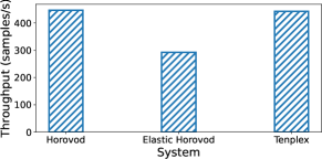
Fig. 17: Training throughput with ResNet50 and ImageNet

Finally, we measure Tenplex’s performance overhead compared to our baselines. We deploy a ResNet50 model with the ImageNet dataset in the on-premise cluster. We measure throughput when training on 2 GPUs.

Fig. 17 shows the throughput (in samples per second) for the Horovod, Elastic Horovod, and Tenplex. Horovod achieves 446 images/s. With elasticity, the throughput drops around a third to 291 images/s. Tenplex has a throughput of 443 images/s—about the same as regular Horovod. Therefore, there is no overhead for Tenplex and an improvement of 34% compared to Elastic Horovod. Tenplex outperforms Horovod Elastic due to its tight integration with the DL system, which instead requires users to explicitly checkpoint states in a blocking manner when changing its configuration.

7 Related Work

Elastic training systems support resource changes but, in contrast with Tenplex, only focus on data parallelism by adding/removing model replicas to GPU workers, while re-partitioning the dataset.

KungFu [33] and Horovod [53] dynamically change the number of workers by adjusting the micro-batch size per worker, keeping the global batch size constant. This requires over-provisioning for the maximum number of workers. In the same vein, DeepPool [42] frees up under-utilized GPUs and allocates them for higher-priority jobs.

Hydrozoa [18] supports static multi-dimensional parallelism before training, but only dynamic change to data parallelism. VirtualFlow [41] leverages the abstraction of virtual nodes to map the models to devices. It splits data batches across virtual nodes for training. Given predefined virtual nodes, VirtualFlow only supports data parallelism below a maximum number of virtual nodes, even though more physical devices are added.

Checkpointing systems store snapshots of model parameters. When resources change (e.g. for failure recovery), the DL system retrieves the latest checkpoint before the failure and resumes training. CheckFreq [36] dynamically adjusts the checkpointing frequency, while Check-N-Run [10] uses lossy compression, trading accuracy for storage efficiency. Similarly, Gemini [62] and Oobleck [25] provide fast checkpointing: while the former stores checkpoints in CPU memory, the latter maintains checkpoints in GPU memory. These approaches, however, focus only on failure recovery, as opposed to the generic runtime reconfiguration enabled by Tenplex.

Distributed training systems execute DL jobs based on a parallelization plan. The plan is generated by a model parallelizer. Alpa [69] searches for an optimal distribution strategy along inter- and intra-operator parallelism; Megatron-LM [55] allows users to specify the distribution plan. Training is performed by DL engines (Tensorflow [1], PyTorch [43], MindSpore [35]) with interfaces to model parallelizers.

8 Conclusion

Current distributed DL systems lack the abstractions to change the parallelization configuration of jobs at runtime. It is an important feature to support elasticity, redeployment, or reconfiguration after failure, it requires a principled approach for the management of the model and dataset state.

We described Tenplex, a dynamic state management library for DL jobs with multi-dimensional parallelism. By describing the state as a parallelizable tensor collection (PTC), Tenplex can generate efficient reconfiguration plans when the underlying GPU resources for the job change at runtime. Its distributed state transformers implement the reconfiguration plan on each GPU with a minimum amount of data movement between workers. Therefore, Tenplex is a step towards making large-scale long-running deep learning jobs fully adaptive to resource changes.

References

- [1] Martín Abadi, Paul Barham, Jianmin Chen, Zhifeng Chen, Andy Davis, Jeffrey Dean, Matthieu Devin, Sanjay Ghemawat, Geoffrey Irving, and Michael Isard. TensorFlow: A System for Large-Scale Machine Learning. In 12th USENIX symposium on operating systems design and implementation (OSDI 16), pages 265–283, 2016.
- [2] Samson B. Akintoye, Liangxiu Han, Xin Zhang, Haoming Chen, and Daoqiang Zhang. A Hybrid Parallelization Approach for Distributed and Scalable Deep Learning. IEEE Access, 10:77950–77961, 2022.
- [3] Amazon. Cloud Object Storage - Amazon S3. https://aws.amazon.com/pm/serv-s3/.
- [4] Sanjith Athlur, Nitika Saran, Muthian Sivathanu, Ramachandran Ramjee, and Nipun Kwatra. Varuna: Scalable, Low-Cost Training of Massive Deep Learning Models. In Proceedings of the Seventeenth European Conference on Computer Systems, EuroSys ’22, page 472–487, New York, NY, USA, 2022. Association for Computing Machinery.
- [5] AWS. SageMaker Distributed Model Parallelism Best Practices. https://docs.aws.amazon.com/sagemaker/latest/dg/model-parallel-best-practices.html.
- [6] Tom B. Brown, Benjamin Mann, Nick Ryder, Melanie Subbiah, Jared Kaplan, Prafulla Dhariwal, Arvind Neelakantan, Pranav Shyam, Girish Sastry, Amanda Askell, Sandhini Agarwal, Ariel Herbert-Voss, Gretchen Krueger, Tom Henighan, Rewon Child, Aditya Ramesh, Daniel M. Ziegler, Jeffrey Wu, Clemens Winter, Christopher Hesse, Mark Chen, Eric Sigler, Mateusz Litwin, Scott Gray, Benjamin Chess, Jack Clark, Christopher Berner, Sam McCandlish, Alec Radford, Ilya Sutskever, and Dario Amodei. Language Models are Few-Shot Learners. In Hugo Larochelle, Marc’Aurelio Ranzato, Raia Hadsell, Maria-Florina Balcan, and Hsuan-Tien Lin, editors, Advances in Neural Information Processing Systems 33: Annual Conference on Neural Information Processing Systems 2020, NeurIPS 2020, December 6-12, 2020, virtual, 2020.
- [7] Jeffrey Dean, Greg Corrado, Rajat Monga, Kai Chen, Matthieu Devin, Quoc V. Le, Mark Z. Mao, Marc’Aurelio Ranzato, Andrew W. Senior, Paul A. Tucker, Ke Yang, and Andrew Y. Ng. Large Scale Distributed Deep Networks. In Peter L. Bartlett, Fernando C. N. Pereira, Christopher J. C. Burges, Léon Bottou, and Kilian Q. Weinberger, editors, Advances in Neural Information Processing Systems 25: 26th Annual Conference on Neural Information Processing Systems 2012. Proceedings of a meeting held December 3-6, 2012, Lake Tahoe, Nevada, United States, pages 1232–1240, 2012.
- [8] J. Deng, W. Dong, R. Socher, L.-J. Li, K. Li, and L. Fei-Fei. ImageNet: A Large-Scale Hierarchical Image Database. In CVPR09, 2009.
- [9] Jacob Devlin, Ming-Wei Chang, Kenton Lee, and Kristina Toutanova. BERT: pre-training of deep bidirectional transformers for language understanding. In Jill Burstein, Christy Doran, and Thamar Solorio, editors, Proceedings of the 2019 Conference of the North American Chapter of the Association for Computational Linguistics: Human Language Technologies, NAACL-HLT 2019, Minneapolis, MN, USA, June 2-7, 2019, Volume 1 (Long and Short Papers), pages 4171–4186. Association for Computational Linguistics, 2019.
- [10] Assaf Eisenman, Kiran Kumar Matam, Steven Ingram, Dheevatsa Mudigere, Raghuraman Krishnamoorthi, Krishnakumar Nair, Misha Smelyanskiy, and Murali Annavaram. Check-N-Run: a Checkpointing System for Training Deep Learning Recommendation Models. In Amar Phanishayee and Vyas Sekar, editors, 19th USENIX Symposium on Networked Systems Design and Implementation, NSDI 2022, Renton, WA, USA, April 4-6, 2022, pages 929–943. USENIX Association, 2022.
- [11] Hadi Esmaeilzadeh, Adrian Sampson, Luis Ceze, and Doug Burger. Neural Acceleration for General-Purpose Approximate Programs. IEEE Micro, 33(3):16–27, 2013.
- [12] Wikimedia Foundation. Wikimedia Downloads. https://dumps.wikimedia.org.
- [13] Patrick Fu. GPU Partitioning: Fair Share Scheduling. https://www.geminiopencloud.com/en/blog/gpu-paritioning-fair-sheduling/, 2022.
- [14] Aaron Gokaslan and Vanya Cohen. OpenWebText Corpus. http://Skylion007.github.io/OpenWebTextCorpus, 2019.
- [15] Google. Google Cloud. https://cloud.google.com/.
- [16] Priya Goyal, Piotr Dollár, Ross B. Girshick, Pieter Noordhuis, Lukasz Wesolowski, Aapo Kyrola, Andrew Tulloch, Yangqing Jia, and Kaiming He. Accurate, Large Minibatch SGD: Training ImageNet in 1 Hour. CoRR, abs/1706.02677, 2017.
- [17] Huifeng Guo, Ruiming Tang, Yunming Ye, Zhenguo Li, and Xiuqiang He. DeepFM: A Factorization-Machine based Neural Network for CTR Prediction. In Carles Sierra, editor, Proceedings of the Twenty-Sixth International Joint Conference on Artificial Intelligence, IJCAI 2017, Melbourne, Australia, August 19-25, 2017, pages 1725–1731. ijcai.org, 2017.
- [18] Runsheng Guo, Victor Guo, Antonio Kim, Josh Hildred, and Khuzaima Daudjee. Hydrozoa: Dynamic Hybrid-Parallel DNN Training on Serverless Containers. In D. Marculescu, Y. Chi, and C. Wu, editors, Proceedings of Machine Learning and Systems, volume 4, pages 779–794, 2022.
- [19] Charles R Harris, K Jarrod Millman, Stéfan J Van Der Walt, Ralf Gommers, Pauli Virtanen, David Cournapeau, Eric Wieser, Julian Taylor, Sebastian Berg, Nathaniel J Smith, et al. Array programming with NumPy. Nature, 585(7825):357–362, 2020.
- [20] Tomoki Hayashi, Ryuichi Yamamoto, Katsuki Inoue, Takenori Yoshimura, Shinji Watanabe, Tomoki Toda, Kazuya Takeda, Yu Zhang, and Xu Tan. Espnet-TTS: Unified, Reproducible, and Integratable Open Source End-to-End Text-to-Speech Toolkit. In 2020 IEEE International Conference on Acoustics, Speech and Signal Processing, ICASSP 2020, Barcelona, Spain, May 4-8, 2020, pages 7654–7658. IEEE, 2020.
- [21] Kaiming He, Xiangyu Zhang, Shaoqing Ren, and Jian Sun. Deep Residual Learning for Image Recognition. In 2016 IEEE Conference on Computer Vision and Pattern Recognition, CVPR 2016, Las Vegas, NV, USA, June 27-30, 2016, pages 770–778. IEEE Computer Society, 2016.
- [22] Marius Hobbhahn and Tamay Besiroglu. Trends in GPU Price-Performance, 2022.
- [23] Horovod. Elastic Horovod. https://horovod.readthedocs.io/en/latest/elastic_include.html.
- [24] Yanping Huang, Youlong Cheng, Ankur Bapna, Orhan Firat, Dehao Chen, Mia Xu Chen, HyoukJoong Lee, Jiquan Ngiam, Quoc V. Le, Yonghui Wu, and Zhifeng Chen. GPipe: Efficient Training of Giant Neural Networks using Pipeline Parallelism. In Hanna M. Wallach, Hugo Larochelle, Alina Beygelzimer, Florence d’Alché-Buc, Emily B. Fox, and Roman Garnett, editors, Advances in Neural Information Processing Systems 32: Annual Conference on Neural Information Processing Systems 2019, NeurIPS 2019, December 8-14, 2019, Vancouver, BC, Canada, pages 103–112, 2019.
- [25] Insu Jang, Zhenning Yang, Zhen Zhang, Xin Jin, and Mosharaf Chowdhury. Oobleck: Resilient Distributed Training of Large Models Using Pipeline Templates. In Jason Flinn, Margo I. Seltzer, Peter Druschel, Antoine Kaufmann, and Jonathan Mace, editors, Proceedings of the 29th Symposium on Operating Systems Principles, SOSP 2023, Koblenz, Germany, October 23-26, 2023, pages 382–395. ACM, 2023.
- [26] Myeongjae Jeon, Shivaram Venkataraman, Amar Phanishayee, Junjie Qian, Wencong Xiao, and Fan Yang. Analysis of Large-Scale Multi-Tenant GPU Clusters for DNN Training Workloads. In 2019 USENIX Annual Technical Conference (USENIX ATC 19), pages 947–960, Renton, WA, July 2019. USENIX Association.
- [27] Zhihao Jia, Matei Zaharia, and Alex Aiken. Beyond Data and Model Parallelism for Deep Neural Networks. Proceedings of Machine Learning and Systems, 1:1–13, 2019.
- [28] Norman P. Jouppi, Cliff Young, Nishant Patil, David A. Patterson, Gaurav Agrawal, Raminder Bajwa, Sarah Bates, Suresh Bhatia, Nan Boden, Al Borchers, Rick Boyle, Pierre-luc Cantin, Clifford Chao, Chris Clark, Jeremy Coriell, Mike Daley, Matt Dau, Jeffrey Dean, Ben Gelb, Tara Vazir Ghaemmaghami, Rajendra Gottipati, William Gulland, Robert Hagmann, C. Richard Ho, Doug Hogberg, John Hu, Robert Hundt, Dan Hurt, Julian Ibarz, Aaron Jaffey, Alek Jaworski, Alexander Kaplan, Harshit Khaitan, Daniel Killebrew, Andy Koch, Naveen Kumar, Steve Lacy, James Laudon, James Law, Diemthu Le, Chris Leary, Zhuyuan Liu, Kyle Lucke, Alan Lundin, Gordon MacKean, Adriana Maggiore, Maire Mahony, Kieran Miller, Rahul Nagarajan, Ravi Narayanaswami, Ray Ni, Kathy Nix, Thomas Norrie, Mark Omernick, Narayana Penukonda, Andy Phelps, Jonathan Ross, Matt Ross, Amir Salek, Emad Samadiani, Chris Severn, Gregory Sizikov, Matthew Snelham, Jed Souter, Dan Steinberg, Andy Swing, Mercedes Tan, Gregory Thorson, Bo Tian, Horia Toma, Erick Tuttle, Vijay Vasudevan, Richard Walter, Walter Wang, Eric Wilcox, and Doe Hyun Yoon. In-Datacenter Performance Analysis of a Tensor Processing Unit. In Proceedings of the 44th Annual International Symposium on Computer Architecture, ISCA 2017, Toronto, ON, Canada, June 24-28, 2017, pages 1–12. ACM, 2017.
- [29] Alex Krizhevsky, Ilya Sutskever, and Geoffrey E. Hinton. ImageNet Classification with Deep Convolutional Neural Networks. In Peter L. Bartlett, Fernando C. N. Pereira, Christopher J. C. Burges, Léon Bottou, and Kilian Q. Weinberger, editors, Advances in Neural Information Processing Systems 25: 26th Annual Conference on Neural Information Processing Systems 2012. Proceedings of a meeting held December 3-6, 2012, Lake Tahoe, Nevada, United States, pages 1106–1114, 2012.
- [30] Jiamin Li, Hong Xu, Yibo Zhu, Zherui Liu, Chuanxiong Guo, and Cong Wang. Aryl: An Elastic Cluster Scheduler for Deep Learning, 2022.
- [31] Mingzhen Li, Wencong Xiao, Biao Sun, Hanyu Zhao, Hailong Yang, Shiru Ren, Zhongzhi Luan, Xianyan Jia, Yi Liu, Yong Li, Depei Qian, and Wei Lin. EasyScale: Accuracy-consistent Elastic Training for Deep Learning, 2022.
- [32] Shen Li, Yanli Zhao, Rohan Varma, Omkar Salpekar, Pieter Noordhuis, Teng Li, Adam Paszke, Jeff Smith, Brian Vaughan, Pritam Damania, and Soumith Chintala. PyTorch distributed. Proceedings of the VLDB Endowment, 13(12):3005–3018, 2020.
- [33] Luo Mai, Guo Li, Marcel Wagenländer, Konstantinos Fertakis, Andrei-Octavian Brabete, and Peter Pietzuch. KungFu: Making Training in Distributed Machine Learning Adaptive. In 14th USENIX Symposium on Operating Systems Design and Implementation (OSDI 20), pages 937–954, 2020.
- [34] Microsoft. Microsoft Azure. https://azure.microsoft.com/.
- [35] MindSpore. Mindspore Deep Learning Training/Inference Framework. https://github.com/mindspore-ai/mindspore, 2020.
- [36] Jayashree Mohan, Amar Phanishayee, and Vijay Chidambaram. CheckFreq: Frequent, Fine-Grained DNN Checkpointing. In 19th USENIX Conference on File and Storage Technologies (FAST 21), pages 203–216, 2021.
- [37] Deepak Narayanan, Aaron Harlap, Amar Phanishayee, Vivek Seshadri, Nikhil R. Devanur, Gregory R. Ganger, Phillip B. Gibbons, and Matei Zaharia. PipeDream: generalized pipeline parallelism for DNN training. In Tim Brecht and Carey Williamson, editors, Proceedings of the 27th ACM Symposium on Operating Systems Principles, SOSP 2019, Huntsville, ON, Canada, October 27-30, 2019, pages 1–15. ACM, 2019.
- [38] Deepak Narayanan, Mohammad Shoeybi, Jared Casper, Patrick LeGresley, Mostofa Patwary, Vijay Korthikanti, Dmitri Vainbrand, Prethvi Kashinkunti, Julie Bernauer, Bryan Catanzaro, Amar Phanishayee, and Matei Zaharia. Efficient large-scale language model training on GPU clusters using megatron-LM. In International Conference for High Performance Computing, Networking, Storage and Analysis, SC 2021, St. Louis, Missouri, USA, November 14-19, 2021, page 58, 2021.
- [39] Bogdan Nicolae, Jiali Li, Justin M. Wozniak, George Bosilca, Matthieu Dorier, and Franck Cappello. DeepFreeze: Towards Scalable Asynchronous Checkpointing of Deep Learning Models. In 20th IEEE/ACM International Symposium on Cluster, Cloud and Internet Computing, CCGRID 2020, Melbourne, Australia, May 11-14, 2020, pages 172–181. IEEE, 2020.
- [40] OpenAi. Introducing ChatGPT. 2022.
- [41] Andrew Or, Haoyu Zhang, and Michael J Freedman. VirtualFlow: Decoupling Deep Learning Models from the Underlying Hardware. arXiv preprint arXiv:2009.09523, 2020.
- [42] Seo Jin Park, Joshua Fried, Sunghyun Kim, Mohammad Alizadeh, and Adam Belay. Efficient Strong Scaling Through Burst Parallel Training. In D. Marculescu, Y. Chi, and C. Wu, editors, Proceedings of Machine Learning and Systems, volume 4, pages 748–761, 2022.
- [43] Adam Paszke, Sam Gross, Francisco Massa, Adam Lerer, James Bradbury, Gregory Chanan, Trevor Killeen, Zeming Lin, Natalia Gimelshein, and Luca Antiga. PyTorch: An Imperative Style, High-Performance Deep Learning Library. Advances in neural information processing systems, 32, 2019.
- [44] Yanghua Peng, Yixin Bao, Yangrui Chen, Chuan Wu, and Chuanxiong Guo. Optimus: An Efficient Dynamic Resource Scheduler for Deep Learning Clusters. In Proceedings of the Thirteenth EuroSys Conference, EuroSys ’18, New York, NY, USA, 2018. Association for Computing Machinery.
- [45] Shashank Prasanna. Train Deep Learning Models on GPUs using Amazon EC2 Spot Instances. https://aws.amazon.com/blogs/machine-learning/train-deep-learning-models-on-gpus-using-amazon-ec2-spot-instances/, 2019.
- [46] PyTorch. Torch Elastic. https://pytorch.org/elastic/latest/.
- [47] Aurick Qiao, Sang Keun Choe, Suhas Jayaram Subramanya, Willie Neiswanger, Qirong Ho, Hao Zhang, Gregory R. Ganger, and Eric P. Xing. Pollux: Co-adaptive Cluster Scheduling for Goodput-Optimized Deep Learning. In Angela Demke Brown and Jay R. Lorch, editors, 15th USENIX Symposium on Operating Systems Design and Implementation, OSDI 2021, July 14-16, 2021. USENIX Association, 2021.
- [48] Alec Radford, Jeff Wu, Rewon Child, David Luan, Dario Amodei, and Ilya Sutskever. Language Models are Unsupervised Multitask Learners. 2019.
- [49] Rajat Raina, Anand Madhavan, and Andrew Y. Ng. Large-scale deep unsupervised learning using graphics processors. In Andrea Pohoreckyj Danyluk, Léon Bottou, and Michael L. Littman, editors, Proceedings of the 26th Annual International Conference on Machine Learning, ICML 2009, Montreal, Quebec, Canada, June 14-18, 2009, volume 382 of ACM International Conference Proceeding Series, pages 873–880. ACM, 2009.
- [50] Samyam Rajbhandari, Conglong Li, Zhewei Yao, Minjia Zhang, Reza Yazdani Aminabadi, Ammar Ahmad Awan, Jeff Rasley, and Yuxiong He. DeepSpeed-MoE: Advancing Mixture-of-Experts Inference and Training to Power Next-Generation AI Scale. In International Conference on Machine Learning, ICML 2022, 17-23 July 2022, Baltimore, Maryland, USA, pages 18332–18346, 2022.
- [51] Samyam Rajbhandari, Jeff Rasley, Olatunji Ruwase, and Yuxiong He. ZeRO: Memory Optimizations Toward Training Trillion Parameter Models. ArXiv, May 2020.
- [52] Jeff Rasley, Samyam Rajbhandari, Olatunji Ruwase, and Yuxiong He. Deepspeed: System optimizations enable training deep learning models with over 100 billion parameters. In Proceedings of the 26th ACM SIGKDD International Conference on Knowledge Discovery and Data Mining, pages 3505–3506, 2020.
- [53] Alexander Sergeev and Mike Del Balso. Horovod: fast and easy distributed deep learning in TensorFlow. arXiv preprint arXiv:1802.05799, 2018.
- [54] Chris Shallue and George Dahl. Measuring the Limits of Data Parallel Training for Neural Networks. https://blog.research.google/2019/03/measuring-limits-of-data-parallel.html, 2019.
- [55] Mohammad Shoeybi, Mostofa Patwary, Raul Puri, Patrick LeGresley, Jared Casper, and Bryan Catanzaro. Megatron-LM: Training Multi-Billion Parameter Language Models Using Model Parallelism. CoRR, abs/1909.08053, 2019.
- [56] Dharma Shukla, Muthian Sivathanu, Srinidhi Viswanatha, Bhargav Gulavani, Rimma Nehme, Amey Agrawal, Chen Chen, Nipun Kwatra, Ramachandran Ramjee, Pankaj Sharma, Atul Katiyar, Vipul Modi, Vaibhav Sharma, Abhishek Singh, Shreshth Singhal, Kaustubh Welankar, Lu Xun, Ravi Anupindi, Karthik Elangovan, Hasibur Rahman, Zhou Lin, Rahul Seetharaman, Cheng Xu, Eddie Ailijiang, Suresh Krishnappa, and Mark Russinovich. Singularity: Planet-Scale, Preemptive and Elastic Scheduling of AI Workloads, 2022.
- [57] Samuel L. Smith and Quoc V. Le. A Bayesian Perspective on Generalization and Stochastic Gradient Descent. In International Conference on Learning Representations, 2018.
- [58] Shaden Smith, Mostofa Patwary, Brandon Norick, Patrick LeGresley, Samyam Rajbhandari, Jared Casper, Zhun Liu, Shrimai Prabhumoye, George Zerveas, Vijay Korthikanti, Elton Zheng, Rewon Child, Reza Yazdani Aminabadi, Julie Bernauer, Xia Song, Mohammad Shoeybi, Yuxiong He, Michael Houston, Saurabh Tiwary, and Bryan Catanzaro. Using DeepSpeed and Megatron to Train Megatron-Turing NLG 530B, A Large-Scale Generative Language Model. CoRR, abs/2201.11990, 2022.
- [59] Christian Szegedy, Vincent Vanhoucke, Sergey Ioffe, Jonathon Shlens, and Zbigniew Wojna. Rethinking the Inception Architecture for Computer Vision. In 2016 IEEE Conference on Computer Vision and Pattern Recognition, CVPR 2016, Las Vegas, NV, USA, June 27-30, 2016, pages 2818–2826. IEEE Computer Society, 2016.
- [60] Colin Unger, Zhihao Jia, Wei Wu, Sina Lin, Mandeep Baines, Carlos Efrain Quintero Narvaez, Vinay Ramakrishnaiah, Nirmal Prajapati, Patrick S. McCormick, Jamaludin Mohd-Yusof, Xi Luo, Dheevatsa Mudigere, Jongsoo Park, Misha Smelyanskiy, and Alex Aiken. Unity: Accelerating DNN Training Through Joint Optimization of Algebraic Transformations and Parallelization. In Marcos K. Aguilera and Hakim Weatherspoon, editors, 16th USENIX Symposium on Operating Systems Design and Implementation, OSDI 2022, Carlsbad, CA, USA, July 11-13, 2022, pages 267–284. USENIX Association, 2022.
- [61] Bharath Kumar Reddy Vangoor, Vasily Tarasov, and Erez Zadok. To FUSE or Not to FUSE: Performance of User-Space File Systems. In 15th USENIX Conference on File and Storage Technologies (FAST 17), pages 59–72, Santa Clara, CA, February 2017. USENIX Association.
- [62] Zhuang Wang, Zhen Jia, Shuai Zheng, Zhen Zhang, Xinwei Fu, T. S. Eugene Ng, and Yida Wang. GEMINI: Fast Failure Recovery in Distributed Training with In-Memory Checkpoints. In Proceedings of the 29th Symposium on Operating Systems Principles, SOSP ’23, page 364–381, New York, NY, USA, 2023. Association for Computing Machinery.
- [63] Qizhen Weng, Wencong Xiao, Yinghao Yu, Wei Wang, Cheng Wang, Jian He, Yong Li, Liping Zhang, Wei Lin, and Yu Ding. MLaaS in the wild: Workload analysis and scheduling in Large-Scale heterogeneous GPU clusters. In 19th USENIX Symposium on Networked Systems Design and Implementation (NSDI 22), pages 945–960, Renton, WA, April 2022. USENIX Association.
- [64] Qizhen Weng, Lingyun Yang, Yinghao Yu, Wei Wang, Xiaochuan Tang, Guodong Yang, and Liping Zhang. Beware of Fragmentation: Scheduling GPU-Sharing Workloads with Fragmentation Gradient Descent. In 2023 USENIX Annual Technical Conference (USENIX ATC 23), pages 995–1008, Boston, MA, July 2023. USENIX Association.
- [65] Yidi Wu, Kaihao Ma, Xiao Yan, Zhi Liu, Zhenkun Cai, Yuzhen Huang, James Cheng, Han Yuan, and Fan Yu. Elastic Deep Learning in Multi-Tenant GPU Clusters. IEEE Transactions on Parallel and Distributed Systems, 33(1):144–158, 2022.
- [66] Wencong Xiao, Romil Bhardwaj, Ramachandran Ramjee, Muthian Sivathanu, Nipun Kwatra, Zhenhua Han, Pratyush Patel, Xuan Peng, Hanyu Zhao, Quanlu Zhang, Fan Yang, and Lidong Zhou. Gandiva: Introspective Cluster Scheduling for Deep Learning. In 13th USENIX Symposium on Operating Systems Design and Implementation (OSDI 18), pages 595–610, Carlsbad, CA, October 2018. USENIX Association.
- [67] Wencong Xiao, Shiru Ren, Yong Li, Yang Zhang, Pengyang Hou, Zhi Li, Yihui Feng, Wei Lin, and Yangqing Jia. AntMan: Dynamic scaling on GPU clusters for deep learning. In 14th USENIX Symposium on Operating Systems Design and Implementation (OSDI 20), pages 533–548. USENIX Association, November 2020.
- [68] Shiwei Zhang, Lansong Diao, Chuan Wu, Siyu Wang, and Wei Lin. Accelerating Large-Scale Distributed Neural Network Training with SPMD Parallelism. In Proceedings of the 13th Symposium on Cloud Computing, SoCC ’22, page 403–418, New York, NY, USA, 2022. Association for Computing Machinery.
- [69] Lianmin Zheng, Zhuohan Li, Hao Zhang, Yonghao Zhuang, Zhifeng Chen, Yanping Huang, Yida Wang, Yuanzhong Xu, Danyang Zhuo, and Joseph E Gonzalez. Alpa: Automating Inter-and Intra-Operator Parallelism for Distributed Deep Learning. arXiv preprint arXiv:2201.12023, 2022.
- [70] Guorui Zhou, Xiaoqiang Zhu, Chengru Song, Ying Fan, Han Zhu, Xiao Ma, Yanghui Yan, Junqi Jin, Han Li, and Kun Gai. Deep Interest Network for Click-Through Rate Prediction. In Yike Guo and Faisal Farooq, editors, Proceedings of the 24th ACM SIGKDD International Conference on Knowledge Discovery & Data Mining, KDD 2018, London, UK, August 19-23, 2018, pages 1059–1068. ACM, 2018.