Can we generate bound-states from resonances or virtual states perturbatively?

Abstract

We investigate whether it is possible to generate bound-states from resonances or virtual states through first-order perturbation theory. Using contact-type potentials as those appeared in pionless effective field theory, we show that it is possible to obtain negative-energy states by sandwiching a next-to-leading order (NLO) interaction with the leading-order (LO) wavefunctions, under the presence of LO resonances or virtual states. However, at least under the framework of time-independent Schrödinger equation and Hermitian Hamiltonian, there is an inability to create bound-states with structure similar to those formed by the non-perturbative treatments.

I Introduction

It is well-known that bound-states correspond to poles in the S-matrix Landau (1995). Under the condition that an interaction contains no pole itself, non-perturbative treatments are required to give rise a pole in the final amplitude. In non-relativistic quantum mechanics, this is usually achieved by treating the interaction as a potential in the Schrödinger or Lippmann-Schwinger equation (LSE). Meanwhile, it could occur that a consistent treatment of interactions under certain frameworks of effective field theory (EFT) involves a non-perturbative treatment of the leading-order (LO) potential, while higher-order corrections are to be added perturbatively under distorted-wave-Born-approximation (DWBA) van Kolck (2020a, b). For example, this occurs in the standard formulation of pionless EFT Hammer et al. (2020) and the modified chiral EFT Kaplan et al. (1998, 1996); Birse (2007); Long and van Kolck (2008); Pavón Valderrama (2011a, b); Long and Yang (2011, 2012a, 2012b); Wu and Long (2019a, b); Peng et al. (2020); Habashi (2022); Thim et al. (2023); Li et al. (2023) approaches to low-energy nuclear physics. Since a LO interaction corresponds to the first approximation in describing a system, it could contain considerable theoretical uncertainty. Under a power counting which prescribes a perturbative arrangement of sub-leading interactions, one demands that the uncertainty of the final observables can always be improved order-by-order perturbatively.

However, one could encounter a situation that a bound-state needed to be restored from an unbound LO result. For example, ¹⁶O is shown to be unstable with respect to decaying into four alpha-particles under pionless EFT at LO Contessi et al. (2017); Bansal et al. (2018) and chiral EFT without three-body forces up to NLO Yang et al. (2021). Though for chiral EFT, a promotion of three-body forces to LO is found based on a combinatorial argument, which fixes the problem of ¹⁶O binding Yang (2020); Yang et al. (2023), it is still of interest to investigate whether it is possible to generate bound-states perturbatively from resonances or virtual states, as this might be demanded if one adopts another theoretical framework or studies other systems. In fact, a recent study suggests that any few-body system obtained by zero-range momentum-independent two-body interactions is unstable against decay into clusters, if its two-body scattering length is much larger than any other scale involved Schäfer et al. (2021). Under this scenario, one must recover the correct pole structure corresponding to physical bound-states through perturbative corrections, at least for systems where the EFT is applicable. However, it is not obvious that this can be achieved easily, as it involves a transition between eigen-states belonging to two different Hilbert spaces.

Since poles are infinities in S-matrix, they cannot be generated from nothing through finite steps of perturbative corrections. The remaining possibility is to convert the resonances or virtual states—which are poles in S-matrix with energies analytic continued to the complex plane—into bound-states. Note that resonance or virtual state poles consist of complex energies and are not eigen-values of a Hermitian Hamiltonian. Under the non-perturbative setting, one could analytic continue the Schrödinger equation or apply methods such as the complex scaling Aguilar and Combes (1971); Balslev and Combes (1971) or other alternatives Horáček and Pichl (2017); Dietz et al. (2022) to extend the domain of the model space. Despite the awful technical difficulty which might prevent one from solving the multi-particle systems in practice, the analytic continued wavefunctions are in principle well-defined.

However, conceptual issues arise once one enters the perturbative regime. First, the S-matrix becomes non-unitary when perturbation theory is applied, which forces the analytic continuation toward a dangerous foundation. The judgement of perturbativity then unavoidably involves comparisons between complex-to-complex or complex-to-real numbers. Thus, the smallness of a perturbative correction—which justifies the convergence of a perturbation series—can be difficult to define in general.

In this work we study the problem within the simplest, Hermitian formalism. It is of interest to check whether bound-states can be generated from resonances or virtual states by straightforwardly applying the first-order perturbation theory, as this is probably the only practical way to be applied numerically in an A-body system with A$\gtrsim 4$. An indirect solution would be to avoid the problem by treating some of the subleading corrections non-perturbatively to “improve” the LO convergence Contessi et al. (2023).

We first layout our methodology of calculation and the condition whether a first-order perturbative correction can be considered as next-to-leading (NLO) under an EFT expansion in Sec. II. Then, in Sec. III, we investigate whether a resonance can be converted to bound-states using the nucleon-nucleon (NN) ³P₀ channel as a testing ground. In Sec. IV, we investigate whether a virtual state can be converted to bound-states using the NN ¹S₀ channel as a testing ground. Then, we discuss a reverse procedure regarding the removal of a LO bound-state and its implications in Sec. V, with a numerical example presented in Sec. VI. The essence of the problem is discussed in Sec. VII. Finally, we summarize our results and skepticize a generalization to many-body systems in Sec. VIII.

II Methodology

II.1 The DWBA formalism

In this work we will assume all interactions are finite-ranged and go to zero in the coordinate space at $r\rightarrow\infty$. In fact, we will analysis the problem in momentum space and adopt interactions decay exponentially after $p\gg\Lambda$, where $\Lambda$ is a momentum cutoff. We will always solve the time-independent Schrödinger or Lippmann-Schwinger equation to generate our LO results non-perturbatively, and then add subleading corrections under DWBA. Denoting $p$ $(p^{\prime})$ the incoming (outgoing) momentum in the center of mass (cm) frame of two equal-mass fermions with mass $M$ ($=939$ MeV in this work), the LO T-matrix regarding their scattering process in an uncoupled partial-wave can be obtained by iterating the LO potential $V_{LO}(p,p^{\prime})$ non-perturbatively in the LSE, i.e.,

$$T_{LO}(p^{\prime},p;E)=V_{LO}(p^{\prime},p)+\frac{2}{\pi}M\int_{0}^{\infty}\frac{dp^{\prime\prime}\;p^{\prime\prime}{}^{2}\;V_{LO}(p^{\prime},p^{\prime\prime})\;T_{LO}(p^{\prime\prime},p,E)}{p_{0}^{2}+i\varepsilon-p^{\prime\prime}{}^{2}},$$ (1)

where $p_{0}^{2}/M=E_{cm}$ is the cm energy. Rewriting Eq. (1) as

$$T_{LO}=V_{LO}+V_{LO}GT_{LO},$$ (2)

with

$$G=\frac{2}{\pi}M\int_{0}^{\infty}\frac{p^{\prime\prime}{}^{2}dp^{\prime\prime}}{p_{0}^{2}+i\varepsilon-p^{\prime\prime}{}^{2}},$$ (3)

the NLO contribution is then given by DWBA and reads Long and Yang (2011)

$$T_{NLO} =V_{NLO}+V_{NLO}GT_{LO}+T_{LO}GV_{NLO}$$

$$+T_{LO}G\,V_{NLO}\,GT_{LO}\,.$$ (4)

where $V_{NLO}$ and $T_{NLO}$ are the interaction and T-matrix at NLO. The LO phase shift $\delta_{LO}$ is related to the LO on-shell T-matrix by

$$\frac{e^{i\delta_{LO}}\sin\delta_{LO}}{-Mp_{0}}=T_{LO}(p_{0},p_{0};E).$$ (5)

Meanwhile, phase shifts up to NLO are in principle to be obtained via a perturbative conversion, since the S-matrix corresponds to $T_{LO}+T_{NLO}$ does not in general present the unitary property. Under the condition that unitarity can be restored order-by-order, the NLO phase shifts $\delta_{NLO}$ can be obtained from $\delta_{LO}$ and $T_{NLO}$ by Long and Yang (2011)

$$T_{NLO}(p_{0},p_{0};E_{cm})=-\delta_{NLO}\frac{e^{2i\delta_{LO}}}{-Mp_{0}}.$$ (6)

On the other hand, Eq. (6) cannot be trusted if it results a $\delta_{NLO}$ far from a real number, which then put the perturbative setting of power counting doubtable in the first place. Once the on-shell T-matrix (at LO or NLO) is obtained, cross section $\sigma$ can be calculated, i.e.,

$$\sigma=4\pi(2l+1)M^{2}|T|^{2},$$ (7)

where $l$ is the angular momentum quantum number of the system and $T=T_{LO}$ ($T_{LO}+T_{NLO}$) for order up to LO (NLO).

Since Eq. (6) is not always valid, one way of just checking whether the energy becomes negative at NLO regardless whether the perturbative setting is consistent or not is to simply calculate the perturbative correction of $V_{NLO}$ by sandwiching it with the LO wavefunctions.

Explicitly, in this work we adopt the Harmonic-Oscillator (HO) basis to diagonalize the LO Hamiltonian

$$H_{LO}=T+V_{LO},$$ (8)

where $T$ denotes the kinetics term. Denoting the $i^{th}$ LO eigen-value and eigen-function as $E_{i}^{LO}$ and $\Psi_{i}^{LO}$, the NLO correction $E_{i}^{NLO}$ is then

$$E_{i}^{NLO}=\langle\Psi_{i}^{LO}|V_{NLO}|\Psi_{i}^{LO}\rangle,$$ (9)

where

$$\Psi_{i}^{LO}=\sum_{n=0}^{n_{max}}C_{in}\psi_{n}^{HO},$$ (10)

and $C_{in}$ denotes the linear combination coefficient of the HO wavefunction $\psi_{n}^{HO}$ up to principle quantum number $n=n_{max}$. One can then check if there is any state with negative energy being generated at NLO, i.e., whether $E_{i}^{LO}+E_{i}^{NLO}<0$.

Note that there are two caveats in the above approach. First, strictly speaking, Eq.(9) is the exact first order perturbative correction of $V_{NLO}$. While in EFT, NLO corrections are associated with an uncertainty up to $O$(NNLO) and do not have an exact value. Thus, even a test based on the above procedure shows that a straightforward perturbative threshold-crossing is problematic, it does not rule out the possibility that adding small additional terms of order $O$(NNLO)—which is allowed by EFT—could overcome the problem. Second, we have approximated the LO eigen-functions—which are scattering waves—in terms of HO basis. These two wavefunctions have different asymptotic behavior and a transition from one to another only exists in the limit $n_{max}\rightarrow\infty$ and under an oscillator strength of the HO function $\hbar\omega\rightarrow 0$. Thus, any unbound to bound transition needed to be analyzed carefully by reducing $\hbar\omega$ and increasing $n_{max}$. Nevertheless, as long as $V^{NLO}$ is finite-range, one only needs to resolute the LO scattering waves by HO basis within the range of $V^{NLO}$ to obtain reliable results of Eq.(9). This can be checked by increasing $n_{max}$ and decreasing $\hbar\omega$ until a convergence is reached.

II.2 An essential difference between perturbative and non-perturbative approaches

When interactions are encoded into potentials, one common expectation is that if $V_{NLO}$ is small compared to $V_{LO}$, the corrections in the final amplitude should be small also, regardless of how it is obtained. Meanwhile, there is an essential difference between the perturbative and non-perturbative approaches.

Within perturbation theory, an eigen-value always consists of its previous order value plus the new corrections, and one can keep track of the evolution of each eigen-state order-by-order. This gives rise to the possibility of tracking the phenomenon of level-crossing—i.e., a lower state can be shifted to a higher state so that a reordering of the energy spectrum occurs. Moreover, the gap between two eigen-states naturally goes through zero when two levels cross each other.

On the other hand, the non-perturbative procedure involves re-diagonalization whenever the potential is changed, and one can only infer how each state evolves. Moreover, it often comes with the so-called avoided-level-crossing feature. As the interacting strength is increased to a critical value, two eigen-states which were initially drawn closer will experience a “sudden jump” and exchange their positions with the gap between them remains finite.

Note that the usual expectation regarding what is “smallness” fails when one approaches the critical region of avoided-level-crossing. To illustrate this point, let us consider a two-level system. At LO, two eigen-states are produced non-perturbatively by an interaction where the strength is just below the critical value. Then, any small correction on top of the LO interaction will produce a profound difference depending on how it is included. On one hand, as long as the increase of the interaction strength is small, the correction should be linear and first order perturbation theory should apply. This will produce a correction which is indeed small and further reduce the gap between the two states. On the other hand, a non-perturbative treatment will trigger the avoided-crossing feature and increases the gap. Thus, normal intuitions no longer hold and one faces the choice between the perturbative and non-perturbative treatments. Ultimately, the choice relies on whether one trusts the expansion in terms of the potentials or the final amplitude. The former calls for a non-perturbative treatment of the interactions and the later demands treating corrections perturbatively. Under the condition that one understands the ultimate interaction or even can produce and fine-tune such potentials experimentally, the non-perturbative treatment should be adopted. Conversely, if the interaction is unclear, then in the spirit of EFT—where the expansion should be arranged order-by-order in terms of the final amplitude—a perturbative treatment is a more natural choice.

It needs to be stressed that any further iteration of a perturbative correction needs not to converge order-by-order toward its non-perturbative correspondence for the perturbative approach to make sense. In fact, a non-perturbative treatment corresponds to adopting a particular set of irreducible diagrams and iterating them to all order, while ignoring all other quantum correction diagrams completely. It is possible that this treatment is inconsistent in the first place. For example, without the entrance of new higher-order diagrams or counter terms, further iterations of $V_{NLO}$ in Eq.(9) could generate non-renormalizable results Long and van Kolck (2008); van Kolck (2020a); Griesshammer (2022); van Kolck (2021), which has been observed also under the presence of finite-range potentials in the context of chiral EFT potentials Nogga et al. (2005); Yang et al. (2009a, b); Zeoli et al. (2013).

However, this also implies that there is an essential difference regarding how eigen-energies are re-distributed between the two approaches, and therefore posts a potential difference between bound-states generated non-perturbatively and bound-states shifted across threshold by perturbation theory. This problem will be encountered in the later sections.

III Resonances to bound-states

In this section we investigate the possibility of perturbatively converting a resonance to bound-states, using the nucleon-nucleon (NN) ³P₀ scattering as a testing ground. A resonance appears when particles are bound temporary and decayed at a later time, which corresponds to a pole in the scattering amplitude with the energy or momentum being analytic continued to the complex plane. It often occurs when an attractive potential has a repulsive “lip” or barrier above $E=0$—due to the angular momentum barrier $l(l+1)/Mr^{2}$—that helps confine the particle Landau (1995); Li et al. (2023).

Breit-Wigner formula can be used to describe the amplitude $f$ near a resonance, i.e.,

$$f=e^{i\delta}\sin\delta=\frac{\Gamma/2}{E_{R}-E-i\Gamma/2},$$ (11)

where $E_{R}$ and $\Gamma$ are the energy and width of the resonance.

In this work we utilize the so-called Argand plot to confirm and extract $E_{R}$ and $\Gamma$ of a resonance.

To generate resonances in the NN ³P₀ channel, we adopt

$$V_{LO}=\left[c_{lo}pp^{\prime}+d_{lo}pp^{\prime}(p^{2}+p^{\prime}{}^{2})\right]f_{R},$$

$$V_{NLO}=\left[c_{nlo}pp^{\prime}+d_{nlo}pp^{\prime}(p^{2}+p^{\prime}{}^{2})\right]f_{R},$$ (12)

where $c_{lo}$, $c_{nlo}$, $d_{lo}$ and $d_{nlo}$ are low-energy constants (LECs), and $V_{LO}$ ($V_{NLO}$) are to be solved non-perturbatively (perturbatively) with a regulator

$$f_{R}=exp\left[-\frac{p^{4}+p^{\prime}{}^{4}}{\Lambda^{4}}\right].$$ (13)

III.1 Case I

We first set $d_{lo}=0$ and $\Lambda=150$ MeV in Eq. (12) and (13). Inserting $c_{lo}=-2.5\times 10^{-9}$ MeV^-4 into Eq. (1) (denoting as case I) gives an Argand plot illustrated in Fig. 1. As the increase of $E=p_{0}^{2}/M$, the complex amplitude $f$ rotates counterclockwise around the circle. As the energy passing through the resonance, $f$ becomes pure imaginary and we extracted $E_{R}=0.53$ MeV and $\Gamma=0.23$ MeV according to Eq. (11). The corresponding phase shifts and differential cross section are plotted as a function of $E_{cm}=T_{lab}/2$ in Fig. 2. Note that, instead of solving the LSE, one could also adopt the HO-basis to diagonalize Eq. (8), and then following the J-matrix method Shirokov et al. (2004, 2005, 2007); Yang (2016) to convert the eigen-energies into scattering phase shifts. We have verified that the same $\delta(^{3}P_{0})$ as listed in the left panel of Fig. 2 can be reproduced by using HO-basis with $\hbar\omega=1$ MeV and $n_{max}=150$.

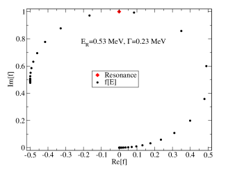
Figure 1: Argand plot (Im[$f$] versus Re[$f$]) of the scattering amplitude $f(p_{0})$ of case I. Starting at origin, an 1 MeV increase in $p_{0}=\sqrt{ME}$ is applied to each point.

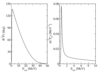
Figure 2: Phase shifts $\delta$ and cross section $\sigma$ as a function of the cm energy $E_{cm}$ at LO of case I.

Next, we add NLO correction. Note that solving LSE with a $10\%$ more attractive $c_{lo}$ (i.e., $c_{lo}$ more negative than $-2.8\times 10^{-9}$ MeV^-4) gives rise a LO bound-state. Thus, as a first test, we adopt only $c_{nlo}pp^{\prime}$ and set $d_{nlo}=0$ in Eq. (12) to see how large the extra effort is to create a bound-state perturbatively against the non-perturbative way. Since the NLO corrections are evaluated with Eq. (9), we first analysis how the results behave with $\hbar\omega$ and $n_{max}$. For each given $\hbar\omega$, the calculation is carried out by increasing $n_{max}$ until the resulting energy spectra converge within $1\%$. Using $c_{lo}=-2.5\times 10^{-9}$ MeV^-4 and $c_{nlo}=-6.0\times 10^{-10}$ MeV^-4, $E^{LO}$ and $E^{NLO}$ obtained from different $\hbar\omega$ are compared in Table 1. As one can see, perturbatively generated negative-energy states are observed when the wavefunctions are constructed by $\hbar\omega\geq 4$ MeV, and disappear when $\hbar\omega=1$ MeV is adopted. Those negative-energy states obtained with $\hbar\omega\geq 4$ MeV should therefore be discarded, as they are merely artifact of using bases consist of bound-state wavefunctions with too large infrared truncation to describe scattering waves. Nevertheless, one observes in Table 1 that the perturbative correction $E_{i}^{NLO}$ always peaked around the index $i$ where $E_{i}^{LO}\sim E_{R}=0.53$ MeV, i.e., the place where LO wavefunction inserted in Eq. (9) is closest to the resonance. Up to this point, two important conclusions can be made. First, although based on the observed trend of reducing $\hbar\omega$, one might always doubt whether an apparent NLO bound-state will disappear if $\hbar\omega$ is further reduced, level-crossing does happen. This is due to the fact that NLO corrections peaked at $E_{R}$, which, when the continuum is discretized by HO-wavefunction with small enough $\hbar\omega$, will always cause states closer to the resonance to receive a larger correction than their nearby states. Then, as long as this correction—which is negative and due to a tunable $V_{NLO}$—exceeds the increasing trend of $E_{i}^{LO}$, a state which was higher at LO will be brought down more than its lower neighbors. Therefore, re-ordering of the energy spectrum from LO to NLO will happen. One can further infer that states with truly negative energies at NLO can be generated under a combination of sufficiently attractive $V_{NLO}$ and closed-enough-to-zero $E_{R}$. However, since a resonance comes with a width $\Gamma$, in the limit $\hbar\omega\rightarrow 0$, the level-crossing will not be limited to only one state. Thus, at least under the setup of case I, continuous states around $E_{R}$ will be brought to bound-states from any resonance with a finite width.

With those caveats in mind, we examine how the NLO results changes with $c_{nlo}$. We adopt $\hbar\omega=1$ MeV and $n_{max}=150$, and plot the NLO corrections in the left panel of Fig. 3. As one expects, the perturbative NLO correction $E^{NLO}_{i}$ is linear to $c_{nlo}$. We then compare the results to those obtained by treating NLO non-perturbatively. Table 2 shows that both the perturbative and non-perturbative generated negative-energy states occur at NLO as the increase of $c_{nlo}$. In this particular case, there is a 4 times difference between the $c_{nlo}$ required to generate a NLO bound-state perturbative versus the case when it is treated non-perturbatively. The corresponding cross sections $\sigma(^{3}P_{0})$ are plotted in Fig. 4.

To see how the pole position of a resonance affects the NLO results, we adopt a less attractive $V_{LO}$ with $c_{lo}=-2\times 10^{-9}$ MeV^-4. This generates a broader resonance which is further away from the threshold with $E_{R}=2.75$ MeV and $\Gamma=2.52$ MeV. The NLO correction are plotted in the right panel of Fig. 3. Note that here we have adopted more attractive $c_{nlo}$ so that for the same legend in the left and right panels, the total strength $c_{lo}+c_{nlo}$ is the same. As one can see, the perturbative corrections become weaker even with more attractive $c_{nlo}$. In fact, we are not able to obtain any bound-state perturbatively up to NLO for all $c_{nlo}$ listed in the right panel of Fig. 3.

i	$\hbar\omega=20$ MeV			$\hbar\omega=10$ MeV
	$E_{i}^{LO}$	$E_{i}^{NLO}$	sum	$E_{i}^{LO}$	$E_{i}^{NLO}$	sum
0	0.48	-0.98	-0.50	0.37	-0.46	-9.20$\times$10-2
1	1.34	-0.58	0.76	0.73	-0.79	-5.87$\times$10-2
2	3.63	-0.34	3.29	1.74	-0.33	1.41
3	7.20	-0.28	6.92	3.37	-0.24	3.13
i	$\hbar\omega=4$ MeV			$\hbar\omega=1$ MeV
	$E_{i}^{LO}$	$E_{i}^{NLO}$	sum	$E_{i}^{LO}$	$E_{i}^{NLO}$	sum
0	0.18	-3.74$\times$10-2	0.15	1.66$\times$10-2	-4.32$\times$10-5	1.65$\times$10-2
1	0.44	-0.58	-0.14	4.89$\times$10-2	-4.16$\times$10-4	4.85$\times$10-2
2	0.73	-0.54	0.19	9.71$\times$10-2	-2.01$\times$10-3	9.51$\times$10-2
3	1.31	-0.26	1.05	0.16	-7.52$\times$10-3	0.15
4	2.12	-0.18	1.94	0.24	-2.56$\times$10-2	0.21
5	3.16	-0.15	3.01	0.33	-8.41$\times$10-2	0.24
6	4.41	-0.14	4.28	0.42	-0.22	0.20
7	5.88	-0.12	5.76	0.52	-0.31	0.21
8	7.58	-0.11	7.46	0.64	-0.24	0.40

Table 1: $E^{LO}_{i}$ and $E^{NLO}_{i}$ obtained with $\hbar\omega=1,4,10,20$ MeV. Perturbatively generated bound-states are marked by bold text. Results are obtained under case I with $c_{lo}=-2.5\times 10^{-9}$ MeV^-4 and $c_{nlo}=-6.0\times 10^{-10}$ MeV^-4.

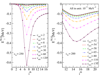
Figure 3: $E^{NLO}_{i}$ obtained perturbatively with various $c_{nlo}$ under $c_{lo}=-2.5\times 10^{-9}$ (left panel) and $c_{lo}=-2\times 10^{-9}$ (right panel) MeV^-4. Note that $\Lambda=150$ MeV and $\hbar\omega=1$ MeV is adopted, therefore all the energies are discretized.

$c_{nlo}$ (MeV-4)	B.S.per (MeV)	B.S.non-per (MeV)
$-2\times 10^{-11}$	N/A	N/A
$-4\times 10^{-11}$	N/A	N/A
$-8\times 10^{-11}$	N/A	N/A
$-15\times 10^{-11}$	N/A	N/A
$-30\times 10^{-11}$	N/A	-0.194
$-60\times 10^{-11}$	N/A	-1.09
$-120\times 10^{-11}$	-0.11, -0.026	-3.19

Table 2: NLO results in ³P₀ channel under case I, obtained via HO-wavefunctions with $\hbar\omega=1$ MeV and $n_{max}=150$. B.S._per (B.S._non-per) is the bound-state energy obtained at NLO when treating Eq. (12) perturbatively (non-perturbatively).

Figure 4: Cross section $\sigma$ as a function of c.m. energy $E_{cm}$ for $c_{nlo}=-2\sim-30\times 10^{-11}$ MeV^-4 in Table 2.

III.2 Case II

Next, we include both the $c_{nlo}$ and $d_{nlo}$ terms in the NLO interaction. Since their first-order perturbative corrections are linear to the prefactor $c_{nlo}$ or $d_{nlo}$, one could define

$$C_{i} =\langle\Psi_{i}^{LO}|pp^{\prime}|\Psi_{i}^{LO}\rangle,$$ (14)

$$D_{i} =\langle\Psi_{i}^{LO}|pp^{\prime}(p^{2}+p^{\prime}{}^{2})|\Psi_{i}^{LO}\rangle,$$ (15)

and Eq. (9) can be rewritten as

$$E_{i}^{NLO}=c_{nlo}C_{i}+d_{nlo}D_{i}.$$ (16)

We now probe the possibility of creating a stand-alone bound-state by a perturbative NLO correction. For each finite $\hbar\omega$ adopted in the HO-wavefunction based calculations, one can always adjust $c_{nlo}$ and $d_{nlo}$ so that $E_{x}^{NLO}+E_{x}^{LO}$ is negative, but its nearest state—which is either $E_{x+1}^{NLO}+E_{x+1}^{LO}$ or $E_{x-1}^{NLO}+E_{x-1}^{LO}$—is positive. This leads to the following equations

$$c_{nlo}A+d_{nlo}B =X,$$

$$c_{nlo}a+d_{nlo}b =Y,$$ (17)

where $A=C_{x}$, $B=D_{x}$, $a=C_{x-1}$, $b=D_{x-1}$ (suppose $x-1$ is the nearest spectrum to $x$). And

$$X =-(E_{x}^{LO}+\sigma),$$

$$Y =-(E_{x-1}^{LO}-\gamma),$$ (18)

with $\sigma,\gamma>0$ so that $E_{x}^{NLO}+E_{x}^{LO}$ is negative and $E_{x-1}^{NLO}+E_{x-1}^{LO}$ is positive. Eq. (17) leads to

$$c_{nlo} =\frac{bX/B-Y}{bA/B-a},$$

$$d_{nlo} =\frac{aX/A-Y}{aB/A-b}.$$ (19)

Now, we investigate the behavior of $c_{nlo}$ and $d_{nlo}$ in the limit $\hbar\omega\rightarrow 0$. In this limit, the spectra become continuous, and the difference between $C_{i}$ and $C_{i-1}$ and $D_{i}$ and $D_{i-1}$ becomes infinitesimal. Thus, they are related by an infinitesimal number $\epsilon>0$:

$$a =A-\epsilon,$$

$$b =B-\epsilon.$$ (20)

On the other hand, for a single bound-state to exist, the energies $X$ and $Y$ must differ by a finite number. Let $\Delta=\sigma+\gamma$ in Eq. (18), one then has

$$Y=X+\Delta,$$ (21)

in the limit $\hbar\omega\rightarrow 0$, where $\Delta>0$ is a finite number. Substituting Eq. (20) and Eq. (21) into Eq. (19), one obtains

$$c_{nlo} =-\frac{\Delta}{\epsilon},$$

$$d_{nlo} =-\frac{\Delta}{\epsilon}.$$ (22)

The above solution blows up in the limit $\hbar\omega\rightarrow 0$. Thus, similar to what happened in case I, unless $E_{R}\rightarrow 0$ or $\Gamma\rightarrow 0$, we are not able to generate a stand-alone bound-state under first-order perturbation theory—a striking difference to the non-perturbative treatment.

We now verify the above conclusion via numerical calculations. We kept $c_{lo}=-2.5\times 10^{-9}$ MeV^-4 and vary $c_{nlo}=2\times 10^{-9}$ to $7\times 10^{-9}$ MeV^-4, $d_{nlo}=-1\times 10^{-13}$ to $-6\times 10^{-13}$ MeV^-6. As one can see in Fig. 5, cascades of negative-energy states appear under the perturbative treatment. In fact, those states are only separated due to the infrared truncation (as a finite $\hbar\omega$ is adopted). This can be inferred from the decrease of binding energies and increase of the number of negative-energy states as one approaches the continuum limit ($\hbar\omega\rightarrow 0$, $n_{max}\rightarrow\infty$). On the other hand, when $V_{LO}+V_{NLO}$ are treated non-perturbatively, a single and deeper bound-state is created within the range $c_{nlo}$ and $d_{nlo}$ tested, and binding energies stay invariant under different $\hbar\omega$.

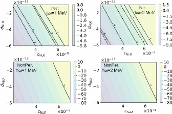
Figure 5: (Upper panels) The lowest state of $E^{LO}+E^{NLO}$ under various $c_{nlo}$ and $d_{nlo}$, where the number of bound-states are given within the contour lines. (Lower panels) Same as the upper panels, but the NLO interaction are treated non-perturbatively.

Note that it is possible to create a sharper resonance at LO by tuning both $c_{lo}$ and $d_{lo}$ listed in Eq. (12). However, we found that as long as $E_{R}$ and $\Gamma$ are finite, the above conclusion persists.

IV Virtual states to bound-states

Virtual states are poles in the (analytic continued) scattering amplitude which occur at momentum $k=i\gamma$ ($\gamma<0$), with the corresponding energies located in the second (unphysical) Riemann sheet Burke (2011). It is well-known that a shallow virtual state exists in the NN ¹S₀ channel, which has been formulated analytically within the pionless EFT already at LO Kaplan et al. (1998, 1996); van Kolck (1999); Sanchez et al. (2018). For example, in standard pionless EFT, one has van Kolck (1999)

$$T_{LO}(k,k;k^{2}/M) \approx\frac{4\pi}{M(1/a+ik-rk^{2}/2+...)}$$

$$\approx\frac{-1}{1/c_{lo}-I_{0}(k)+...},$$ (23)

where $a$ and $r$ are the scattering length and effective range, “…” stands for higher-order contribution, and

$$I_{0}(k)=-\frac{M}{2\pi^{2}}[\theta\Lambda+i\frac{\pi}{2}k+\frac{k^{2}}{\Lambda}O(\frac{k^{2}}{\Lambda^{2}})],$$ (24)

where $\theta$ is a positive number, and $\theta\Lambda=\Lambda$ if a sharp cutoff $\Lambda$ replaces the regulator listed in Eq. (13). Thus, as long as $a<0$ and $r>0$, the pole of the above T-matrix occurs at $k=i\gamma$ with $\gamma<0$, which then corresponds to a virtual state. When $a\rightarrow-\infty$, this virtual state moves to the threshold.

In the following, we use NN ¹S₀ scattering as a testing ground and adopt

$$V_{LO} =c_{lo}f_{R},$$

$$V_{NLO} =[c_{nlo}+d_{nlo}(p^{2}+p^{\prime}{}^{2})]f_{R},$$ (25)

to investigate the possibility of converting a virtual state to bound-state perturbatively. At LO, we adopted $c_{lo}=-4.7\times 10^{-6}$ MeV^-2 and $f_{R}$ as listed in Eq. (13) with $\Lambda=450$ MeV. Solving this $V_{LO}$ in LSE gives $a=-24$ fm, $r=0.81$ fm, with the corresponding phase shifts and cross section plotted in Fig. 6.

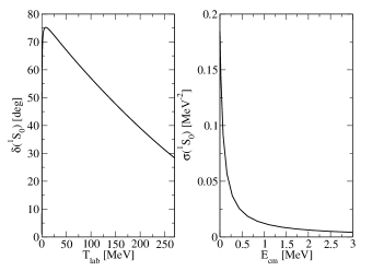
Figure 6: Phase shifts $\delta$ and cross section $\sigma$ as a function of laboratory energy $T_{lab}=2E_{cm}$ at LO for $c_{lo}=-4.7\times 10^{-6}$ MeV^-2 and $\Lambda=450$ MeV.

To investigate the NLO contribution, we again adopt a small $\hbar\omega=1$ MeV and evaluate Eq. (9). With $d_{nlo}=0$ and $c_{nlo}$ made increasingly attractive, results analog to Table 2 are listed in Table 3. One can see that Table 3 resembles what happened in the ³P₀ channel, i.e., a virtual state is converted to a series of bound-states as $V_{NLO}$ is made more attractive. $E^{NLO}_{i}$ and the total energy up to NLO correspond to the most attractive case in Table 3 are plotted as Fig. 7. Once again, the NLO correction peaked around the index $x$ where $E^{LO}_{x}$ is close to the energy of the virtual state.

$c_{nlo}$ (MeV-2)	B.S.per ($10^{-3}$ MeV)	B.S.non-per (MeV)
$-1\times 10^{-7}$	N/A	N/A
$-2\times 10^{-7}$	N/A	$-7.5\times 10^{-4}$
$-5\times 10^{-7}$	N/A	-0.21
$-10\times 10^{-7}$	N/A	-1.2
$-15\times 10^{-7}$	-1.13, -1.61	-2.9
$-20\times 10^{-7}$	-2.9, -7.8, -7.2	-5.1

Table 3: NLO results in ¹S₀ channel under $c_{lo}=-4.7\times 10^{-6}$ MeV^-2 and $\Lambda=450$ MeV. Results are obtained via HO-wavefunctions with $\hbar\omega=1$ MeV and $n_{max}=250$. B.S._per (B.S._non-per) is the bound-state energy obtained at NLO when treating Eq. (12) perturbatively (non-perturbatively).

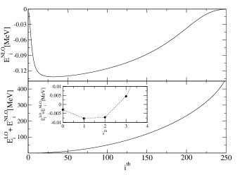
Figure 7: $E^{NLO}_{i}$ (upper panel) and $E^{LO}_{i}+E^{NLO}_{i}$ (lower panel) under $c_{lo}=-4.7\times 10^{-6}$ MeV^-2 $c_{nlo}=-20\times 10^{-7}$ MeV^-2 and $\Lambda=450$ MeV. The first four energies of the lower panel are magnified in the inset. Note that $\hbar\omega=1$ MeV is adopted, therefore all the energies are discretized.

Next, we consider both $c_{nlo}$ and $d_{nlo}$. We kept $V_{LO}$ the same and vary $c_{nlo}=1\times 10^{-6}$ to $5\times 10^{-5}$ MeV^-2, $d_{nlo}=-2\times 10^{-11}$ to $-5.2\times 10^{-10}$ MeV^-4. Results are presented in Fig. 8. As one can see, cascades of bound-states appear in a way similar to the NN ³P₀ case. On the other hand, when $V_{LO}+V_{NLO}$ are treated non-perturbatively, a single and deeper bound-state is created and the binding energies stay invariant under different $\hbar\omega$.

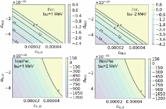
Figure 8: (Upper panels) The lowest state of $E^{LO}+E^{NLO}$ under various $c_{nlo}$ and $d_{nlo}$, where the number of bound-states are given within the contour lines. (Lower panels) Same as the upper panels, but the NLO interaction are treated non-perturbatively.

V A reverse case

Considering now a scenario where a bound-state is generated from a non-perturbative treatment of the LO interaction, and one wishes to remove it at NLO perturbatively. A repulsive $V_{NLO}$ is then required in this case, and its contribution is again given by Eq. (9). Only now the eigen-function corresponds to the LO bound-state can be easily represented by HO-wavefunctions as they are of the same type. In fact, since the LO bound-state wavefunction and $V_{NLO}$ have more overlap within finite distance, one can easily design a scenario that the required NLO energy-shift to lift the LO bound-state are small so that the corresponding $V_{NLO}$ required is much smaller than $V_{LO}$. Thus, everything appear to be well-defined within perturbation theory.

However, there is still a problem. The bound-state lifted from LO will now join the continuum at NLO. Thus, there will be two states correspond to one energy in the NLO continuum spectrum—one belongs to a state which is shifted upward from the LO continuum, the other is the LO bound-state which contains a pole. In general, with the presence of resonances or virtual states, level-crossing within the continuum spectrum can happen from LO to NLO under perturbation theory, where one can always find two different states coincide at NLO as they can receive unequal energy shifts with the difference equals to their LO gap. This degeneracy is not a problem as long as their wavefunctions evaluated up to NLO only differ by higher-order components. However, the coincidence of the lifted bound-state to another continuum state poses several conceptual difficulties. First, it is not entirely clear whether the NLO wavefunction of the lifted bound-state is in presence of bound or continuum property. Moreover, the T-matrix at this energy is degenerated with a difference much more than what higher-orders in perturbation theory can account for. I.e., one is finite and the other has a pole. Note that this pole presences a particular feature, as in its nearby energy region, the T-matrix does not have the trend to become divergent at all. Thus, this state must be categorized as an unphysical state and be discarded, even though the shift from LO to NLO can be completely legal within perturbation theory. On the other hand, poles of this type are exactly what we needed in the previous two sections in order to create stand-alone bound-states perturbatively. We do not claim that this type of poles is the only one to be used to create problem-free bound-states perturbatively. Unfortunately, this is the most straightforward and probably the only scenario which is numerically possible for $A>4$ systems.

VI A numerical example of lifting the leading order bound-state

We now present an example regarding the removal of LO bound-states as postulated in Sec. V. Under the NN ³P₀ case and $\Lambda=150$ MeV in Eq. (13), adopting $V_{LO}=c_{lo}pp^{\prime}$ with $c_{lo}=-2.8\times 10^{-9}$ MeV^-4 will gives a LO bound-state with binding energy $E^{LO}_{0}=-0.194$ MeV. Then, we add a $V_{NLO}$ which has the same structure as $V_{LO}$ but is 35 times weaker, i.e., $c_{nlo}=8\times 10^{-11}$ MeV^-4 and $d_{nlo}=0$ as listed in Eq. (12). In this case, the LO bound-state receives a perturbative lift $\sim 0.211$ MeV and join the continuum at NLO. Note that if the same $c_{nlo}$ is added non-perturbatively, the correction from LO to NLO is $0.197$ MeV.

In Table 4, the perturbative and non-perturbative results are compared with $c_{nlo}$ ranging from $5\times 10^{-11}$ to $8\times 10^{-11}$ MeV^-4. As one can see, at least up to $8\times 10^{-11}$ MeV^-4, the energy shift received by the LO bound-state can be considered small, as the non-perturbative results can be approximated perturbatively with an error well-below $10\%$.

$c_{nlo}$ (MeV-4)	$E^{NLO}_{0}$ (MeV)	$E^{NLO}_{non-per,0}$ (MeV)
$5\times 10^{-11}$	0.132	0.127
$6\times 10^{-11}$	0.159	0.151
$7\times 10^{-11}$	0.185	0.175
$8\times 10^{-11}$	0.211	0.197

Table 4: The perturbative versus non-perturbative NLO shifts to the LO bound-state, where results are obtained in the NN ³P₀ channel under $c_{lo}=-2.8\times 10^{-9}$ MeV^-4 and $c_{nlo}$ with values listed above. Calculations here converge within $0.1\%$ with the decrease of $\hbar\omega$ and increase of $n_{max}$.

However, cross sections obtained perturbatively and non-perturbatively up to NLO show another story, where a big difference between the two NLO treatments is presented at $E_{cm}\sim 0.0026$ MeV as shown in Fig. 9. Note that the perturbative amplitude up to NLO are generated from $T_{LO}(p_{0},p_{0};E_{cm})$ with $E_{cm}>0$, so the NLO results do not contain the state converted from the LO pole. As a result, the perturbative generated cross section is smooth against $E_{cm}$ without particular feature presented around the energy of the lifted pole $E_{cm}=E^{LO}_{0}+E^{NLO}_{0}\sim 0.017$ MeV. On the other hand, a sharp resonance is generated via the non-perturbative treatment with its full shape around the peak re-plotted in the right pannel of Fig. 9. The difference between the two NLO treatments are rather small after $E_{cm}>1$ MeV. Moreover, the change from LO to NLO is $\lessapprox 15\%$, which suggests that perturbation theory works very well in this region. However, the mis-match between results obtained perturbatively and non-perturbatively at $E_{cm}<1$ MeV suggests that even we can make a case where the NLO interaction is arbitrarily small compared to $V_{LO}$, as long as it involves a sign change in the pole position, there will be an energy domain where a perturbative expansion of the final observables fails.

The lesson we learnt from the above case can be summarized as the following. If an energy-shift from LO to NLO involves bound to/from unbound transitions, but the observables one wishes to describe do not involve the problematic part of this conversion, then an order-by-order converged expansion under perturbation theory can still hold. On the other hand, there is always a domain where the correction from $V_{NLO}$ is not small. After all, a continuum to bound-state transition is a violent configuration change.

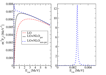
Figure 9: Cross section $\sigma$ as a function of c.m. energy $E_{cm}$ corresponds to the last row of Table 4, where the LO+NLO_non-per results (blue dots) are re-plotted in the right panel in order to show its full amplitude around the peak.

VII Essence of the problem

Results in the above sections show that, although a transition between bound and unbound states can be achieved by perturbative corrections, the outcome is not necessarily desirable.

Since any unbound to/from bound transition needs to go through the threshold, the problem can be reduced into whether the threshold can be (or how well it can be) produced perturbatively. In the following we consider the simplest case consists of only two particles. Note that for $E>0$, physical states consist of scattering states—which are continuous in $E$. On the other hand, for $E<0$, there are discretized bound-states. Now, consider the situation where the interaction is made just attractive enough so that an $E=-|\epsilon|$ state is produced. When this is produced non-perturbatively, it presences an unique and universal feature—i.e., the so-called unitarity or scale-invariance feature Hammer and Platter (2007); Braaten and Hammer (2006); Griesshammer and van Kolck (2023); van Kolck (2019, 2018, 2017); König et al. (2017). Under this limit, the scattering length is much larger than all other scales and the system can be generated by a simple contact potential. Note that due to the avoided-crossing phenomenon, no continuous bound-state can be generated. On the other hand, several problems could occur when the unitarity limit needed to be obtained through perturbation theory. First, there is no guarantee that when the threshold-crossing happens (i.e, when $E=-|\epsilon|$ is first generated), the scattering length is automatically infinity. This can be understood by rewriting the NLO potential to be evaluated within first order perturbation theory as $\chi v_{nlo}$, where $\chi$ is an adjustable number denoting the overall strength and $v_{nlo}$ concerns the form of the interaction. There are various combinations of $\chi$ and $v_{nlo}$ which give the same $\langle\Psi_{i}^{LO}|\chi v_{nlo}|\Psi_{i}^{LO}\rangle$. However, this freedom also means various scales can enter and the unique feature of scale-invariance at unitarity limit does not hold in general if the threshold is approached solely via the first order perturbation theory. Second, at least under Schrödinger equation—where the amplitudes are summed non-relativistic—the unitarity of the S-matrix is no longer exact under the perturbative treatment. Thus, any physical observables evaluated perturbatively within DWBA will in general presence an imaginary component. Normally this does not pose a problem, as if the perturbation is justified, the non-unitary part will be small compared to the full results. However, when a bound-state is just created after the occurrence of threshold-crossing, any non-vanishing imaginary component in $E$ will be much larger compared to $|\epsilon|$, so that the unitarity of S-matrix is severely violated. Since the Riemann sheet where resonances reside is connected to the one where bound-states belong to only through the origin, any defect with respect to the exact threshold will result in the presence of continuous bound-states as seen in the previous sections.

Thus, unless one chooses a very specific $v_{nlo}$ and/or applies additional procedures to ensure that the unitarity is well-reproduced at threshold, the two approaches (perturbative v.s. non-perturbative) will generate results with very different structure—even within the energy domain where the corrections are small in both cases.

VIII Summary and implications to many-body systems

In this work we have tested the possibility of generating bound-states perturbatively. Though numerical calculations are performed only on several selective examples, our results can be very general and will hold as long as: (i) the interactions are finite-ranged; (ii) the problem can be evaluated under time-independent Schrödinger equation—where all eigen-values are real number.

Our investigation suggests the following:

• Under the existence of resonances or virtual states—which are generated non-perturbatively at LO—corrections in energy due to a perturbative insertion of NLO interaction peak at the resonance energy or the momentum corresponds to the pole position of the virtual state. Therefore, re-ordering of the original eigen-states happens, and since level-crossing is allowed, it is possible to convert resonances and virtual states to negative-energy states perturbatively.

• However, in contrast to the non-perturbative treatment, a straightforward implementation of DWBA will generally result in a series of perturbatively created negative-energy states (or to be interpreted as a bound-state with non-zero width).

• On the other hand, an attempt to remove a LO bound-state perturbatively also leads to disagreements with respect to the non-perturbative results, at least in some particular energy domain.

• Therefore, moving a pole perturbatively across the threshold (which corresponds to a transition between the unphysical and physical sheets) requires extra cares. In general, a stand alone ground-state cannot be produced by simply applying the first-order perturbation theory.

Our study in two-particle systems suggests the following generalization for an $A$-particle system. Suppose after solving $V_{LO}$ non-perturbatively, an $A$-particle system consists a bound sub-system with $(A-x)$ particles and $x$ free particles. Then, by adding $V_{NLO}$ perturbatively, one could easily make the $(A-x)$ sub-system more bound (provided that $V_{NLO}$ is an $n$-body force with $n\leq A-x$). Therefore, it could appear that the total binding energy of the system can be shifted to any desired value. However, a change in the pole structure—which requires the adherence between the $(A-x)$ sub-system and $x$ free particles—is unlikely to happen without creating a cascade of bound-states.

In summary, with the caveat that the perturbative correction examined in this work is just a subset of a perturbative EFT-power counting, we conclude that it is possible to generate negative-energy states perturbatively under the presence of resonances or virtual states at the previous order. However, a discretized spectrum of bound-states is unlikely to be generated in this way, unless the width of the previous pole approaches zero.

Acknowledgements. We thank D. Gazda for the assistance during various stage of this work, J. Mares, T. Dytrych and D. Phillips for useful discussions. This work is partially stimulated from the (on-line) discussion of INT workshop—Nuclear Forces for Precision Nuclear Physics (INT-21-1b). This work was supported by the the Extreme Light Infrastructure Nuclear Physics (ELI-NP) Phase II, a project co-financed by the Romanian Government and the European Union through the European Regional Development Fund - the Competitiveness Operational Programme (1/07.07.2016, COP, ID 1334); the Romanian Ministry of Research and Innovation: PN23210105 (Phase 2, the Program Nucleu); the ELI-RO grant Proiectul ELI12/16.10.2020 of the Romanian Government; and the Czech Science Foundation GACR grant 19-19640S and 22-14497S. We acknowledge PRACE for awarding us access to Karolina at IT4Innovations, Czechia under project number EHPC-BEN-2023B05-023 (DD-23-83 and DD-23-157); IT4Innovations at Czech National Supercomputing Center under project number OPEN24-21 1892; Ministry of Education, Youth and Sports of the Czech Republic through the e-INFRA CZ (ID:90140) and CINECA HPC access through PRACE-ICEI standard call 2022 (P.I. Paolo Tomassini).

References

- Landau (1995) Rubin H. Landau, Quantum Mechanics II (Wiley, 1995).
- van Kolck (2020a) U. van Kolck, “The Problem of Renormalization of Chiral Nuclear Forces,” Front. in Phys. 8, 79 (2020a), arXiv:2003.06721 [nucl-th] .
- van Kolck (2020b) U. van Kolck, “Naturalness in nuclear effective field theories,” Eur. Phys. J. A 56, 97 (2020b), arXiv:2003.09974 [nucl-th] .
- Hammer et al. (2020) H.-W. Hammer, S. König, and U. van Kolck, “Nuclear effective field theory: status and perspectives,” Rev. Mod. Phys. 92, 025004 (2020), arXiv:1906.12122 [nucl-th] .
- Kaplan et al. (1998) David B. Kaplan, Martin J. Savage, and Mark B. Wise, “Two-nucleon systems from effective field theory,” Nuclear Physics B 534, 329–355 (1998).
- Kaplan et al. (1996) David B. Kaplan, Martin J. Savage, and Mark B. Wise, “Nucleon-nucleon scattering from effective field theory,” Nuclear Physics B 478, 629–659 (1996).
- Birse (2007) Michael C. Birse, “Deconstructing triplet nucleon-nucleon scattering,” Phys. Rev. C 76, 034002 (2007), arXiv:0706.0984 [nucl-th] .
- Long and van Kolck (2008) B. Long and U. van Kolck, “Renormalization of Singular Potentials and Power Counting,” Annals Phys. 323, 1304–1323 (2008), arXiv:0707.4325 [quant-ph] .
- Pavón Valderrama (2011a) M. Pavón Valderrama, “Perturbative renormalizability of chiral two pion exchange in nucleon-nucleon scattering,” Phys. Rev. C 83, 024003 (2011a), arXiv:0912.0699 [nucl-th] .
- Pavón Valderrama (2011b) M. Pavón Valderrama, “Perturbative Renormalizability of Chiral Two Pion Exchange in Nucleon-Nucleon Scattering: P- and D-waves,” Phys. Rev. C 84, 064002 (2011b), arXiv:1108.0872 [nucl-th] .
- Long and Yang (2011) Bingwei Long and C. J. Yang, “Renormalizing chiral nuclear forces: a case study of 3P0,” Phys. Rev. C 84, 057001 (2011), arXiv:1108.0985 [nucl-th] .
- Long and Yang (2012a) Bingwei Long and C. J. Yang, “Renormalizing Chiral Nuclear Forces: Triplet Channels,” Phys. Rev. C 85, 034002 (2012a), arXiv:1111.3993 [nucl-th] .
- Long and Yang (2012b) Bingwei Long and C. J. Yang, “Short-range nuclear forces in singlet channels,” Phys. Rev. C 86, 024001 (2012b), arXiv:1202.4053 [nucl-th] .
- Wu and Long (2019a) Shaowei Wu and Bingwei Long, “Perturbative scattering in chiral effective field theory,” Phys. Rev. C 99, 024003 (2019a), arXiv:1807.04407 [nucl-th] .
- Wu and Long (2019b) Shaowei Wu and Bingwei Long, “Perturbative scattering in chiral effective field theory,” Phys. Rev. C 99, 024003 (2019b), arXiv:1807.04407 [nucl-th] .
- Peng et al. (2020) Rui Peng, Songlin Lyu, and Bingwei Long, “Perturbative chiral nucleon–nucleon potential for the partial wave,” Commun. Theor. Phys. 72, 095301 (2020), arXiv:2011.13186 [nucl-th] .
- Habashi (2022) J. B. Habashi, “Nucleon-nucleon scattering with perturbative pions: The uncoupled P-wave channels,” Phys. Rev. C 105, 024002 (2022), arXiv:2107.13666 [nucl-th] .
- Thim et al. (2023) Oliver Thim, Eleanor May, Andreas Ekström, and Christian Forssén, “Bayesian analysis of chiral effective field theory at leading order in a modified Weinberg power counting approach,” Phys. Rev. C 108, 054002 (2023), arXiv:2302.12624 [nucl-th] .
- Li et al. (2023) Qingfeng Li, Songlin Lyu, Chen Ji, and Bingwei Long, “Effective field theory with resonant P-wave interaction,” Phys. Rev. C 108, 024002 (2023), arXiv:2303.17292 [nucl-th] .
- Contessi et al. (2017) L. Contessi, A. Lovato, F. Pederiva, A. Roggero, J. Kirscher, and U. van Kolck, “Ground-state properties of 4 he and 16 o extrapolated from lattice QCD with pionless EFT,” Phys. Lett. B 772, 839–848 (2017).
- Bansal et al. (2018) A. Bansal, S. Binder, A. Ekström, G. Hagen, G. R. Jansen, and T. Papenbrock, “Pion-less effective field theory for atomic nuclei and lattice nuclei,” Phys. Rev. C 98, 054301 (2018), arXiv:1712.10246 [nucl-th] .
- Yang et al. (2021) C. J. Yang, A. Ekström, C. Forssén, and G. Hagen, “Power counting in chiral effective field theory and nuclear binding,” Phys. Rev. C 103, 054304 (2021), arXiv:2011.11584 [nucl-th] .
- Yang (2020) C. J. Yang, “Do we know how to count powers in pionless and pionful effective field theory?” Eur. Phys. J. A 56, 96 (2020), arXiv:1905.12510 [nucl-th] .
- Yang et al. (2023) C. J. Yang, A. Ekström, C. Forssén, G. Hagen, G. Rupak, and U. van Kolck, “The importance of few-nucleon forces in chiral effective field theory,” Eur. Phys. J. A 59, 233 (2023), arXiv:2109.13303 [nucl-th] .
- Schäfer et al. (2021) M. Schäfer, L. Contessi, J. Kirscher, and J. Mareš, “Multi-fermion systems with contact theories,” Phys. Lett. B 816, 136194 (2021), arXiv:2003.09862 [nucl-th] .
- Aguilar and Combes (1971) J. Aguilar and J. M. Combes, “A class of analytic perturbations for one-body schrödinger hamiltonians,” Communications in Mathematical Physics 22, 269–279 (1971).
- Balslev and Combes (1971) E. Balslev and J. M. Combes, “Spectral properties of many-body schrödinger operators with dilatation-analytic interactions,” Communications in Mathematical Physics 22, 280–294 (1971).
- Horáček and Pichl (2017) Jiří Horáček and Lukáš Pichl, “Calculation of resonance s-matrix poles by means of analytic continuation in the coupling constant,” Communications in Computational Physics 21, 1154–1172 (2017).
- Dietz et al. (2022) Sebastian Dietz, Hans-Werner Hammer, Sebastian König, and Achim Schwenk, “Three-body resonances in pionless effective field theory,” Phys. Rev. C 105, 064002 (2022), arXiv:2109.11356 [nucl-th] .
- Contessi et al. (2023) Lorenzo Contessi, Martin Schäfer, and Ubirajara van Kolck, “Improved action for contact effective field theory,” (2023), arXiv:2310.15760 [physics.atm-clus] .
- Gasparyan and Epelbaum (2023) A. M. Gasparyan and E. Epelbaum, ““Renormalization-group-invariant effective field theory” for few-nucleon systems is cutoff dependent,” Phys. Rev. C 107, 034001 (2023), arXiv:2210.16225 [nucl-th] .
- (32) C. J. Yang, “A further study on the renormalization-group aspect of perturbative corrections (in preparation).” .
- von Neumann and Wigner (1993) J von Neumann and E P Wigner, “Über merkwürdige diskrete eigenwerte,” in The Collected Works of Eugene Paul Wigner (Springer Berlin Heidelberg, Berlin, Heidelberg, 1993) pp. 291–293.
- Landau and Lifshitz (1981) L D Landau and E M Lifshitz, Quantum mechanics, 3rd ed., edited by John Menzies (Butterworth-Heinemann, Oxford, England, 1981).
- Madison et al. (2012) Kirk W Madison, Yiqiu Wang, Ana Maria Rey, and Kai Bongs, Annual Review of Cold Atoms and Molecules (WORLD SCIENTIFIC, 2012).
- Griesshammer (2022) Harald W. Griesshammer, “What Can Possibly Go Wrong?” Few Body Syst. 63, 44 (2022), arXiv:2111.00930 [nucl-th] .
- van Kolck (2021) U. van Kolck, “Nuclear Effective Field Theories: Reverberations of the Early Days,” Few Body Syst. 62, 85 (2021), arXiv:2107.11675 [nucl-th] .
- Nogga et al. (2005) A. Nogga, R. G. E. Timmermans, and U. van Kolck, “Renormalization of one-pion exchange and power counting,” Phys. Rev. C 72, 054006 (2005), arXiv:nucl-th/0506005 .
- Yang et al. (2009a) C. J. Yang, Ch. Elster, and Daniel R. Phillips, “Subtractive renormalization of the chiral potentials up to next-to-next-to-leading order in higher NN partial waves,” Phys. Rev. C 80, 034002 (2009a), arXiv:0901.2663 [nucl-th] .
- Yang et al. (2009b) C. J. Yang, Ch. Elster, and D. R. Phillips, “Subtractive renormalization of the NN interaction in chiral effective theory up to next-to-next-to-leading order: S waves,” Phys. Rev. C 80, 044002 (2009b), arXiv:0905.4943 [nucl-th] .
- Zeoli et al. (2013) Ch Zeoli, R Machleidt, and D R Entem, “Infinite-cutoff renormalization of the chiral nucleon–nucleon interaction up to n3lo,” Few-body Syst. 54, 2191–2205 (2013).
- Shirokov et al. (2004) A. M. Shirokov, A. I. Mazur, S. A. Zaytsev, J. P. Vary, and T. A. Weber, “Nucleon nucleon interaction in the J matrix inverse scattering approach and few nucleon systems,” Phys. Rev. C 70, 044005 (2004), arXiv:nucl-th/0312029 .
- Shirokov et al. (2005) A. M. Shirokov, J. P. Vary, A. I. Mazur, S. A. Zaytsev, and T. A. Weber, “Novel N N interaction and the spectroscopy of light nuclei,” Phys. Lett. B 621, 96–101 (2005), arXiv:nucl-th/0407018 .
- Shirokov et al. (2007) A. M. Shirokov, J. P. Vary, A. I. Mazur, and T. A. Weber, “Realistic Nuclear Hamiltonian: ’Ab exitu’ approach,” Phys. Lett. B 644, 33–37 (2007), arXiv:nucl-th/0512105 .
- Yang (2016) C. J. Yang, “Chiral potential renormalized in harmonic-oscillator space,” Phys. Rev. C 94, 064004 (2016), arXiv:1610.01350 [nucl-th] .
- Burke (2011) Philip George Burke, R-Matrix Theory of Atomic Collisions (Springer Berlin Heidelberg, 2011).
- van Kolck (1999) U. van Kolck, “Effective field theory of short range forces,” Nucl. Phys. A 645, 273–302 (1999), arXiv:nucl-th/9808007 .
- Sanchez et al. (2018) M. Sánchez Sanchez, C.-J. Yang, Bingwei Long, and U. Van Kolck, “Two-nucleon s01 amplitude zero in chiral effective field theory,” Phys. Rev. C 97 (2018), 10.1103/physrevc.97.024001.
- Hammer and Platter (2007) H. W. Hammer and L. Platter, “Universal Properties of the Four-Body System with Large Scattering Length,” Eur. Phys. J. A 32, 113–120 (2007), arXiv:nucl-th/0610105 .
- Braaten and Hammer (2006) Eric Braaten and H. W. Hammer, “Universality in few-body systems with large scattering length,” Phys. Rept. 428, 259–390 (2006), arXiv:cond-mat/0410417 .
- Griesshammer and van Kolck (2023) Harald W. Griesshammer and Ubirajara van Kolck, “Universality of Three Identical Bosons with Large, Negative Effective Range,” (2023), arXiv:2308.01394 [nucl-th] .
- van Kolck (2019) U. van Kolck, “Nuclear physics with an effective field theory around the unitarity limit,” Nuovo Cim. C 42, 52 (2019).
- van Kolck (2018) U. van Kolck, “Nuclear physics from an expansion around the unitarity limit,” J. Phys. Conf. Ser. 966, 012014 (2018).
- van Kolck (2017) U. van Kolck, “Unitarity and Discrete Scale Invariance,” Few Body Syst. 58, 112 (2017).
- König et al. (2017) Sebastian König, Harald W. Grießhammer, H. W. Hammer, and U. van Kolck, “Nuclear Physics Around the Unitarity Limit,” Phys. Rev. Lett. 118, 202501 (2017), arXiv:1607.04623 [nucl-th] .