Engineering synthetic gauge fields through the coupling phases in cavity magnonics

Abstract

Cavity magnonics, which studies the interaction of light with magnetic systems in a cavity, is a promising platform for quantum transducers, quantum memories, and devices with non-reciprocal behaviour. At microwave frequencies, the coupling between a cavity photon and a magnon, the quasi-particle of a spin wave excitation, is a consequence of the Zeeman interaction between the cavity’s magnetic field and the magnet’s macroscopic spin. For each photon/magnon interaction, a coupling phase factor exists, but is often neglected in simple systems. However, in “loop-coupled” systems, where there are at least as many couplings as modes, the coupling phases become relevant for the physics and lead to synthetic gauge fields. We present experimental evidence of the existence of such coupling phases by considering two spheres made of Yttrium-Iron-Garnet and two different re-entrant cavities. We predict numerically the values of the coupling phases, and we find good agreement between theory and the experimental data. Theses results show that in cavity magnonics, one can engineer synthetic gauge fields, which can be useful for building nonreciprocal devices.

I Introduction

Magnons are the quasi-particles associated with the elementary excitation of a spin wave in a magnetically ordered material, such as the ferrimagnet Yttrium-Iron-Garnet (YIG). The field of cavity magnonics, or spin cavitronics, aims to use the interaction of photons in a cavity with magnons for both classical (e.g. radio-frequency circulators or isolators, and spintronics [1, 2, 3, 4, 5, 6, 7, 8, 9, 10]) and quantum technologies [11, 12, 13]. Magnons are notably promising for quantum transduction [14], due to their capability to couple to phonons [15], optical and microwave photons, and superconducting qubits [16, 17, 18, 19]. The coupling with microwave photons has been particularly fruitful, with demonstrations of coherent coupling [20], indirect coupling [21, 22], ultrastrong coherent coupling [23, 24, 25, 26, 27], dissipative coupling [28, 29, 30, 31, 32, 33, 34, 35, 36], non-reciprocal effects [36, 37, 38, 39], the tuning between level repulsion and attraction [40, 41], and a dark mode memory [42].

Physically, all of these results involve the photon/magnon coupling, which originates from the Zeeman interaction between the magnetic dipole moment of the magnet, and the magnetic field. This interaction is characterised by a coupling strength and a coupling phase, which can both be chosen real positive numbers. In most simple systems, the coupling phases can be ignored since they do not affect the physics. However, in “loop-coupled” systems [37, 43, 44, 45, 46, 47, 48], where there are at least as many couplings as modes, neglecting the coupling phases can lead to an erroneous description of the physics. Indeed in these systems, the various coupling phases (each due to a photon/magnon interaction) combine to form synthetic $U(1)$ gauge fields characterised by a unique gauge-invariant phase $\theta$. These synthetic gauge fields induce a synthetic magnetic field, which is an essential ingredient to break time-reversal symmetry and create non-reciprocal behaviours [45, 46, 47, 48, 49, 50].

Recently, the influence of the coupling phases was theoretically analysed in a loop-coupled system [51] consisting of two magnon modes coupling to two cavity modes, however without experimental verification. To bridge this gap, we propose two re-entrant three-post cavities, in which multiple cavity modes simultaneously couple to two magnon modes. We experimentally measure a first cavity in which the physics is characterised by a single physical phase $\theta=\pi$, which makes it fall within the theoretical analysis of the previous work [51]. In contrast, in the second cavity, the physics is determined by two physical phases $\theta_{1}=0$ and $\theta_{2}=\pi$. In both cavities, we predict theoretically the values of the physical phases, and find good agreement with our experiments.

In section II, we introduce the coupling phases, and how one can reduce them to the so-called physical phases characterising the physics using unitary transformations. Next, in section III, we introduce a cavity with a physical phase $\theta=\pi$, which is supported by both theory and experiment. In section IV, we perform a similar analysis, but this time on a cavity leading to physical phases $\theta_{1}=\pi$ and $\theta_{2}=0$. We conclude in section V.

II Introduction to the magnon/photon coupling phase

We adopt a second-quantised formalism for the description of the cavity (annihilation operator $c_{k}$) and magnon modes (annihilation operator $m_{l}$ after performing the Holstein-Primakoff transformation [52] on the macrospin operator [53]). The ferromagnetic resonance frequency of the magnons is tuned by a static applied magnetic field $\mathbf{H}_{0}=H_{0}\hat{\mathbf{z}}$. The coupling between the cavity mode $c_{k}$ and the magnon mode $m_{l}$ is characterised by a coupling strength $g_{kl}/2\pi$ and a coupling phase $\varphi_{kl}$ defined as [53, 51]

$$g_{kl}/2\pi=\eta_{kl}\sqrt{\omega_{k}}\frac{\gamma}{4\pi}\sqrt{\frac{\mu}{g_{L}\mu_{B}}\hbar\mu_{0}n_{s}},$$ (1)

$$\varphi_{kl}=\arg\quantity{\int_{V_{m}}\differential[3]{r}\mathbf{h}_{k}(\mathbf{r})\cdot\hat{\mathbf{x}}+i\int_{V_{m}}\differential[3]{r}\mathbf{h}_{k}(\mathbf{r})\cdot\hat{\mathbf{y}}},$$ (2)

where $\gamma/2\pi=28$ GHz/T is the gyromagnetic ratio, $\mu=5\mu_{B}$ is the magnetic moment of a unit cell of YIG, $\mu_{B}$ is the Bohr magneton, $\mu_{0}$ is the magnetic permeability of vacuum, $g_{L}=2$ is the Landé $g$-factor, $n_{s}=4.22\times 10^{23}$ m^-3 is the spin density of YIG [54], $\mathbf{h}_{k}$ is the magnetic field vector of the cavity mode $k$, $V_{m}$ is the volume of the YIG spheres, and

$$\eta_{kl}=\sqrt{\frac{\quantity(\int_{V_{m}}\differential[3]{r}\mathbf{h}_{k}(\mathbf{r})\cdot\hat{\mathbf{x}})^{2}+\quantity(\int_{V_{m}}\differential[3]{r}\mathbf{h}_{k}(\mathbf{r})\cdot\hat{\mathbf{y}})^{2}}{V_{m}\int_{V_{c}}\differential[3]{r}\absolutevalue{\mathbf{h}_{k}(\mathbf{r})}^{2}}}$$ (3)

is the filling-factor, with $V_{c}$ the volume of the cavity. The interaction Hamiltonian between the cavity mode $c_{k}$ and the magnon mode $m_{l}$ reads [51]

$$H_{I}=\hbar g_{kl}\quantity(e^{i\varphi_{kl}}c_{k}m_{l}^{\dagger}+e^{-i\varphi_{kl}}c_{k}^{\dagger}m_{l}).$$ (4)

where we used the rotating wave approximation, which is valid provided $\frac{g_{kl}}{\omega_{k}}<10\%$ [55, 56]. Note that the interaction Hamiltonian eq. 4 is Hermitian, and results for the coherent coupling between photons and magnons. This is in stark contrast with dissipative couplings [11, 12], when the interaction is non-Hermitian and results from an indirect coupling [49] of the magnon and photons through a strongly dissipative mode [28, 29], or travelling wave reservoir [36, 30, 31, 32, 33, 34, 35].

Formally, recall that the unitary transformation $U=e^{i\varphi c^{\dagger}c}$ transforms the operator $c$ as $c\mapsto e^{-i\varphi}c$, and that unitary transformations amount to a change of basis. Thus, the transformations $U_{c_{k}}=e^{i\varphi_{kl}c_{k}^{\dagger}c_{k}}$ and $U_{m_{l}}=e^{-i\varphi_{kl}m_{l}^{\dagger}m_{l}}$ can both remove the coupling phase from eq. 4. Physically, this means that there exists a basis in which the coupling phase vanishes, so we might as well set it to zero to simplify the study of the physics. In other words, this amounts to changing the reference phase.

The situation is more complicated when one considers several simultaneous couplings. Naturally, any isolated bosonic mode has a local phase degree of freedom (corresponding to a $U(1)$ symmetry), since e.g. the mapping $c\mapsto e^{-i\varphi}c$ does not change its Hamiltonian. However, couplings between modes constrain these local phase choices, which can break this symmetry. For instance, the coupling of eq. 4 “locks” the local phase choices of $c_{k}$ and $m_{l}$ together, but we are still free to rotate either $c_{k}$ (using $U_{c_{k}}$) or $m_{l}$ (using $U_{m_{l}}$) to remove the coupling phase. In other words, we have two phase degrees of freedom, but only one constraint between them. However, when the number of couplings (constraints) is greater or equal to the number of modes (degrees of freedom), then we cannot remove all the coupling phases, and they become relevant for the physics.

To illustrate this concept, let us consider the example of two magnon modes simultaneously coupling to three cavity modes, as illustrated in fig. 1. We can eliminate the coupling phases between $m_{1}$ and the cavity modes in fig. 1(a) using

$$U_{c_{k}}=e^{i\varphi_{k1}c_{k}^{\dagger}c_{k}},\quad k\in\quantity{1,2,3},$$ (5)

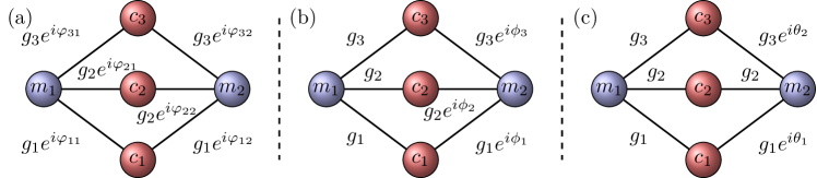
((a))

((b))

((c))

Figure 1: Simplification of the physics of a system composed of two magnon modes $m_{1}$ and $m_{2}$ (in blue) coupling equally and simultaneously to three cavity modes $c_{1},c_{2}$ and $c_{3}$ (in red). (a) The system where all the coupling phases remain. (b) After unitarily transforming the cavity modes using eq. 5, the physics is determined only by three phases $\phi_{k}=\varphi_{k2}-\varphi_{k1}$, accounting for the difference in coupling for each cavity mode $k\in\quantity{1,2,3}$. (c) After rotating $m_{2}$ using eq. 6, we are left with two physical phases $\theta_{1}=\phi_{1}-\phi_{2}$ and $\theta_{2}=\phi_{3}-\phi_{2}$.

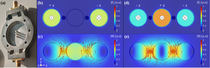
((a))

((b))

((c))

((d))

((e))

Figure 2: (a) The three-posts re-entrant cavity $\pi$ used in the experiment. The lid of the cavity is not shown. (b-c) Electric and magnetic field norm simulated using COMSOL Multiphysics^® of the first eigenmode $c_{1}$ (frequency $\omega_{c,1}/2\pi=4.524$ GHz) of cavity $\pi$. (d-e) Electric and magnetic field distribution simulated using COMSOL of the second eigenmode $c_{2}$ (frequency $\omega_{c,2}/2\pi=6.378$ GHz) of cavity $\pi$. For each mode, the magnetic field is maximal between the posts, where the YIG spheres are placed, while the electric field is concentrated between the top of the posts and the lid of the cavity. The vectors are only shown for the magnetic field

and we obtain fig. 1(b). Next, we rotate $m_{2}$ with

$$U_{c_{k}}=e^{i\phi_{2}m_{2}^{\dagger}m_{2}},$$ (6)

and finally obtain two physical phases $\theta_{1}$ and $\theta_{2}$ characterising the physics (see fig. 1(c)).

Therefore, in the system of fig. 1, we have six couplings and five modes, leading to two physical phases. If the two magnons couple to only two cavity modes (e.g. by setting $g_{3}=0$), we have as many constraints as degrees of freedom, and the system is characterised by a single physical phase.

III A single physical phase

Cavity design

The first cavity we consider, called cavity $\pi$, is pictured in fig. 2(a), and contains three posts. It is based on the design of a two-post re-entrant cavity from ref [23, 24], and possesses similar eigenmodes. The distribution of the magnetic field of the two cavity eigenmodes of interest was simulated using COMSOL Multiphysics^® (see figs. 2(c) and 2(e)). The magnetic field of these two cavity eigenmodes are concentrated between the posts, where we place two identical YIG spheres of diameter 470 $\mu$m. Importantly, the magnetic field of the eigenmodes is either in the same or opposite directions at the sphere locations, which leads to different coupling phases. This difference can also be understood by considering the strength and direction of the electric field, which is concentrated between the top of the posts and the lid (see figs. 2(b) and 2(d)). For instance, the electric field of the first cavity eigenmode (see fig. 2(b)) is localised only on the left and right posts, but with opposing directions (which by the right-hand rule, agrees with the circulation of the magnetic field shown in fig. 2(c)). Conversely, for the second cavity eigenmode, the electric field is non-zero on top of each posts, albeit with different intensities and orientations, and thus leads to the magnetic field of fig. 2(e).

Table 1: Numerical calculation of the coupling strengths $g_{kl}$ and coupling phases $\varphi_{kl}$ of cavity $\pi$ using COMSOL.

Coupling strength (MHz)		Coupling phase (radians)
$g_{11}/2\pi$	139	$\varphi_{11}$	$-\frac{\pi}{2}$
$g_{12}/2\pi$	139	$\varphi_{12}$	$-\frac{\pi}{2}$
$g_{21}/2\pi$	207	$\varphi_{21}$	$+\frac{\pi}{2}$
$g_{22}/2\pi$	207	$\varphi_{22}$	$-\frac{\pi}{2}$

Prediction of the physical phase

The numerical evaluation of the coupling strengths and coupling phases (given by eqs. 1 and 2) can be performed using the eigenmode analysis of COMSOL Multiphysics^®, the results of which are summarised in table 1. Recall that the first index corresponds to the cavity mode, while the second is for the magnon mode. For the magnon modes, $l=1$ ($l=2$) corresponds to the left (right) YIG sphere. We first note that the coupling phases indeed follow the direction of the two cavity eigenmodes’s magnetic field shown in fig. 2. Furthermore, we observe that both YIG spheres couple with the same coupling strength to each cavity mode, as can be expected from the symmetry of the problem. Hence from now on we set $g_{11}=g_{12}=g_{1}$ and $g_{21}=g_{22}=g_{2}$. Assuming both YIG spheres to be perfectly identical, the Hamiltonian of the system is $H_{\pi}=H_{\text{free}}+H_{I}$ with

$$H_{\text{free}}=\sum_{k=1}^{2}\hbar\omega_{c,k}c_{k}^{\dagger}c_{k}+\sum_{l=1}^{2}\hbar\omega_{m}m_{l}^{\dagger}m_{l}$$ (7)

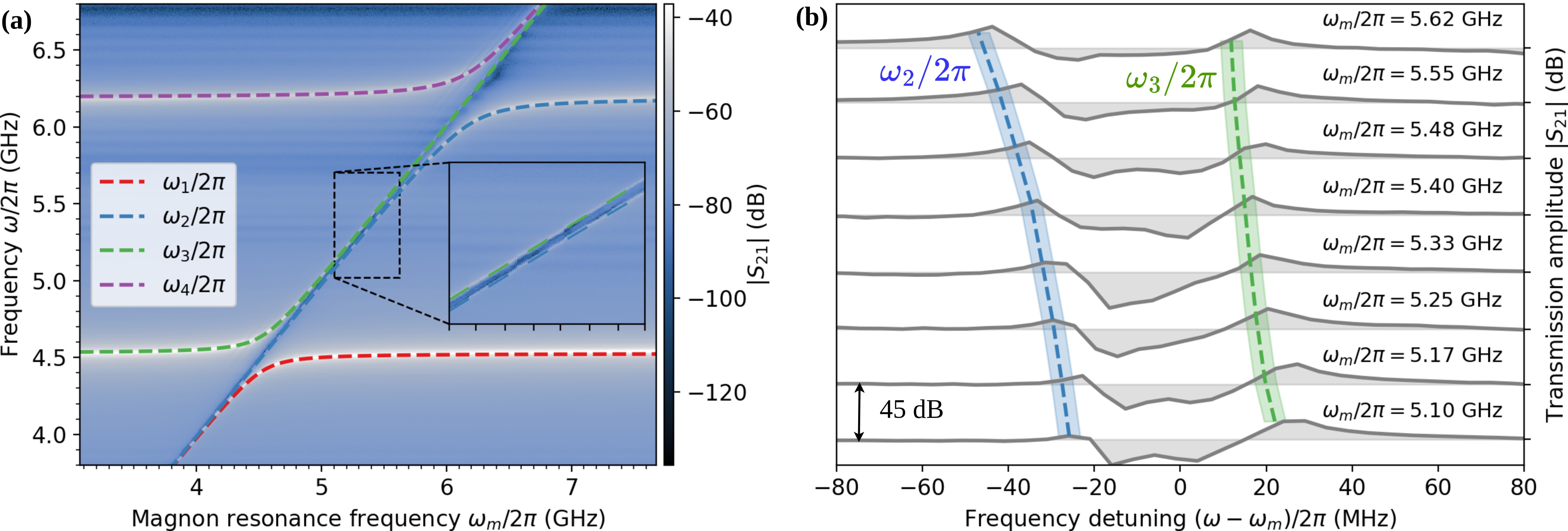
((a))

((b))

Figure 3: (a) Experimental transmission amplitude $\absolutevalue{S_{21}}$ of the cavity $\pi$, along with the theoretical spectrum in dashed lines. The fit parameters are $\omega_{c,1}/2\pi=4.527$ GHz, $\omega_{c,2}/2\pi=6.19$ GHz , $g_{1}/2\pi=81$ MHz, $g_{2}/2\pi=120$ MHz, and $\theta_{1}=\pi$. Inset: zoom for $5.1\leq\omega_{m}/2\pi\leq 5.62$ GHz, and $5.02\leq\omega/2\pi\leq 5.7$ GHz, showing that the hybridised photon-magnon polariton frequencies $\omega_{2}/2\pi$ and $\omega_{3}/2\pi$ do not cross. The ticks indicate the $\omega_{m}/2\pi$ cuts plotted in (b). (b) Line cuts for different values of $\omega_{m}/2\pi$ of the transmission amplitude $\absolutevalue{S_{21}}$ with the spectrum in dashed lines. The width of $\omega_{/}2\pi$ and $\omega_{3}/2\pi$ show the uncertainty $\pm 2.5$ MHz in frequency. For each line cut, the average value of the transmission is used to define the horizontal line from which the colouring begins: this allows to distinguish between resonances and anti-resonances. All the transmission line cuts are separated by 45 dB. The legend for the spectrum is common to (a) and (b).

where $\omega_{m}=\gamma H_{0}$ is the ferromagnetic resonance frequency of the lowest-order magnon modes (Kittel mode) and

$$H_{I} =\;\hbar g_{1}e^{-i\frac{\pi}{2}}c_{1}m_{1}^{\dagger}+\hbar g_{1}e^{-i\frac{\pi}{2}}c_{1}m_{2}^{\dagger}$$ (8)

$$\quad+\hbar g_{2}e^{i\frac{\pi}{2}}c_{2}m_{1}^{\dagger}+\hbar g_{2}e^{-i\frac{\pi}{2}}c_{2}m_{2}^{\dagger}+\mathrm{h.c}$$

with $\mathrm{h.c}$ indicating the hermitian conjugate terms. This system falls within the example of fig. 1 by setting $g_{3}=0$, from which we deduce that after the unitary transformations, the interaction Hamiltonian can be written as

$$H_{I} =\hbar g_{1}c_{1}m_{1}^{\dagger}+\hbar g_{1}e^{i\theta_{1}}c_{1}m_{2}^{\dagger}$$ (9)

$$\quad\hbar g_{2}c_{2}m_{1}^{\dagger}+\hbar g_{2}c_{2}m_{2}^{\dagger}+\mathrm{h.c},$$

with $\theta_{1}=\varphi_{12}-\varphi_{11}-\quantity(\varphi_{22}-\varphi_{21})=\pi$, hence the name “cavity $\pi$” for the cavity.

The values of the coupling strengths and of the physical phase can be verified by the transmission amplitude $\absolutevalue{S_{21}}$ through the cavity. Hence in appendix A we performed a frequency domain simulation using COMSOL to numerically compute $\absolutevalue{S_{21}}$ as a function of the magnon resonance frequency $\omega_{m}/2\pi$, and we obtained good agreement with the eigenmode results of table 1.

Experimental results

The three-post cavity $\pi$ design was 3D-printed and then metallised. Using a vector network analyser, we measured the transmission through the cavity when the static magnetic field $\mathbf{H}_{0}$ is swept to tune $\omega_{m}$, and we obtained the data in fig. 3. The hybridised photon-magnon polariton frequencies are predicted by the spectrum of $H_{\pi}=H_{\text{free}}+H_{I}$, with $H_{\text{free}}$ given by eq. 7 and $H_{I}$ given by eq. 9, is plotted on top of the colour map with $\theta_{1}=\pi$ as suggested by table 1, but with adjusted parameters $g_{1}/2\pi=81$ MHz and $g_{2}/2\pi=120$ MHz instead. We attribute the difference between theory and experiment for the coupling strengths to the imperfection of the 3D-printing and metallisation processes. In particular, the posts of cavity $\pi$ are not completely cylindrical which changes the focusing of the magnetic field between the two posts.

Nevertheless, we note that while the observed coupling strengths are lower than the theoretical values, the prediction for $\theta_{1}$ remains valid. Indeed, as shown in [51], for $\theta_{1}=0$ the frequencies $\omega_{2}/2\pi$ and $\omega_{3}/2\pi$ cross, while for $\theta_{1}=\pi$ they do not. Figure 3(b) and the inset of fig. 3(a) confirm the existence of a frequency gap between $\omega_{2}/2\pi$ and $\omega_{3}/2\pi$, which is the signature of the indirect coupling between both magnons [51]. In other words, this spectral feature demonstrates the coherent coupling between two spatially distant YIG spheres mediated by the two cavity modes, despite the relatively high frequency detuning. Note that if we had $\theta_{1}=0$ instead, the cavity-mediated magnon-magnon coupling would interfere destructively.

The coherent coupling of a cavity mode to two YIG spheres leads to an enhancement of $\sqrt{2}$ of the frequency gap at the anticrossings, i.e. the gap is given by $2\sqrt{2}g$ instead of $2g$ [51, 57], which we verified in appendix B by comparing with measurements with a single YIG sphere.

IV Analysis of two physical phases

Cavity $\pi 0$ design

Using cavity $\pi$, we showed the existence of a single physical phase $\theta_{1}=\pi$. In this section, we examine the possibility of obtaining a different value for the physical phase. In the previous cavity, the origin of the difference in circulation of the magnetic field between the posts can be understood by examining the distribution of the electric field. Following this principle, we engineered another 3-posts re-entrant cavity to obtain two different values $\theta=0$ and $\theta=\pi$ for the physical phases in a unique cavity. This is achieved by making the radius of the centre post (0.75 mm) larger than that of the other two posts (0.5 mm), as shown in fig. 4. As a result of this difference in the radii, the electric field intensity is stronger on the centre post compared to the other two (see fig. 4(a)). This leads to the appearance of another cavity eigenmode of frequency $\omega_{c,2}/2\pi=7.525$ GHz in which the magnetic field distribution solely rotates around the centre post as shown in fig. 4(b). Interestingly, the other two cavity eigenmodes observed for cavity $\pi$ remain, but their frequencies is modified as $\omega_{c,1}/2\pi\mapsto\omega_{c,1}/2\pi=6.544$ GHz and $\omega_{c,2}/2\pi\mapsto\omega_{c,3}/2\pi=8.567$ GHz.

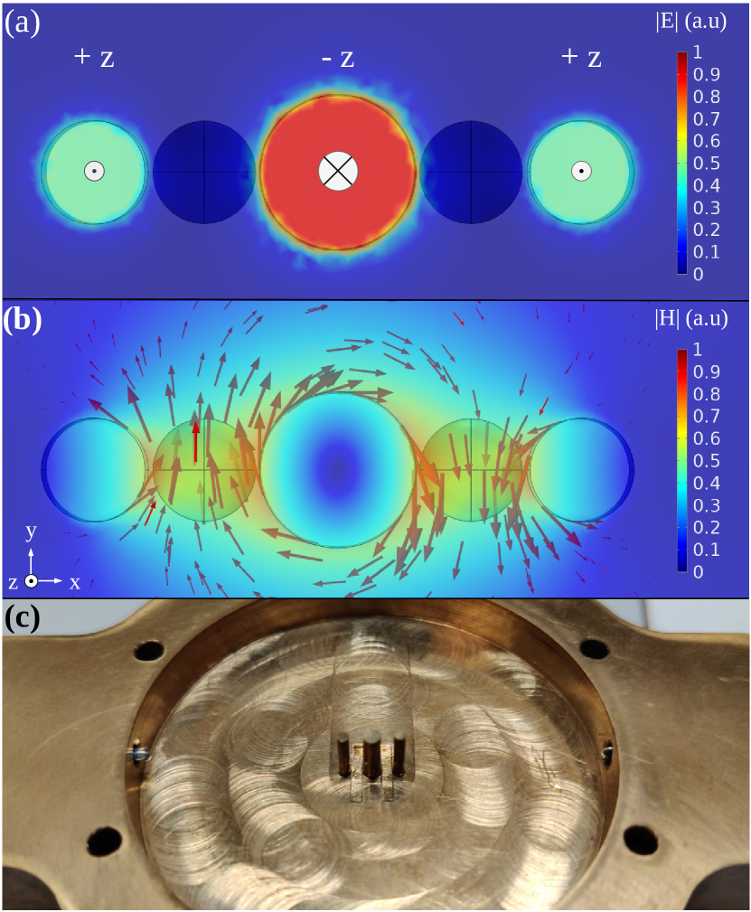
((a))

((b))

((c))

Figure 4: Electric (a) and magnetic (b) field distribution simulated using COMSOL Multiphysics^® of the second eigenmode $c_{2}$ of cavity $\pi 0$. The two eigenmodes of cavity $\pi$ still exist but have different frequencies. (c) The three-posts re-entrant cavity $\pi 0$. Contrary to cavity $\pi$, the three posts do not have the same radius, leading to the creation of an additional cavity mode shown in (a) and (b).

Prediction of the physical phases

Table 2: Numerical calculation of the coupling strengths $g_{kl}$ and coupling phases $\varphi_{kl}$ of cavity $\pi 0$ using COMSOL.

Coupling strength (MHz)		Coupling phase (radians)
$g_{11}/2\pi$	130	$\varphi_{11}$	$-\frac{\pi}{2}$
$g_{12}/2\pi$	127	$\varphi_{12}$	$-\frac{\pi}{2}$
$g_{21}/2\pi$	148	$\varphi_{21}$	$+\frac{\pi}{2}$
$g_{22}/2\pi$	150	$\varphi_{22}$	$-\frac{\pi}{2}$
$g_{31}/2\pi$	103	$\varphi_{31}$	$+\frac{\pi}{2}$
$g_{32}/2\pi$	104	$\varphi_{32}$	$-\frac{\pi}{2}$

The resulting system consists of three cavity eigenmodes, each coupling to the two YIG spheres. The coupling strengths and coupling phases are computed using COMSOL, with the results listed in table 2. Once again, given the symmetry of the problem, both YIG spheres couple with almost equal coupling strength to each cavity eigenmode, so we set $g_{11}=g_{12}=g_{1}=130$ MHz, $g_{21}=g_{22}=g_{2}=150$ MHz and $g_{31}=g_{32}=g_{3}=104$ MHz. The system thus obtained is that described in section II, and using fig. 1 we deduce that the physics is characterised by two coupling phases $\theta_{1}$ and $\theta_{2}$. Using table 2, we predict $\theta_{1}=\varphi_{12}-\varphi_{11}-\quantity(\varphi_{22}-\varphi_{21})=\pi$ and $\theta_{2}=\varphi_{32}-\varphi_{31}-\quantity(\varphi_{22}-\varphi_{21})=0$, hence the “$\pi 0$” cavity. The frequency-domain simulation is plotted in appendix A and agrees with the eigenmode analysis of table 2.

Experimental results

For cavity $\pi$ of section III, we did not have a precise qualitative agreement with the theoretical predictions due to the additive manufacturing process of the cavity. Thus, we adopted a different strategy for cavity $\pi 0$: we used brass cylinders with a calibrated height to implement the posts, and we machined the rest of the cavity from brass. In re-entrant cavities, the eigenmodes are very sensitive to the distance between the top of the posts and the lid. Hence, by using posts with identical heights, we ensure that the potential error in the distance between the posts and the lid is uniform.

The experimental data, along with the polariton spectrum, is plotted in fig. 5. This time, the fit parameters exactly correspond to those given in table 2, which indicates that the construction of the cavity matches very well with the COMSOL design. As for the cavity $\pi$, the physical phase $\theta_{1}=\pi$ suggests that the eigen-frequencies do not cross between the first two anti-crossings, which is indeed confirmed by fig. 5(b). On the other hand, having $\theta_{2}=0$ should lead to a crossing of the eigen-frequencies between the second and third anti-crossings [51]. However when $\theta_{2}=0$ one of the polaritons is a magnonic dark mode [42, 51], which does not lead to a resonance in the transmission amplitude [57]. Thus, as observed in fig. 5(c), we merely observe a single resonance peak moving as $\omega_{m}/2\pi$ is varied.

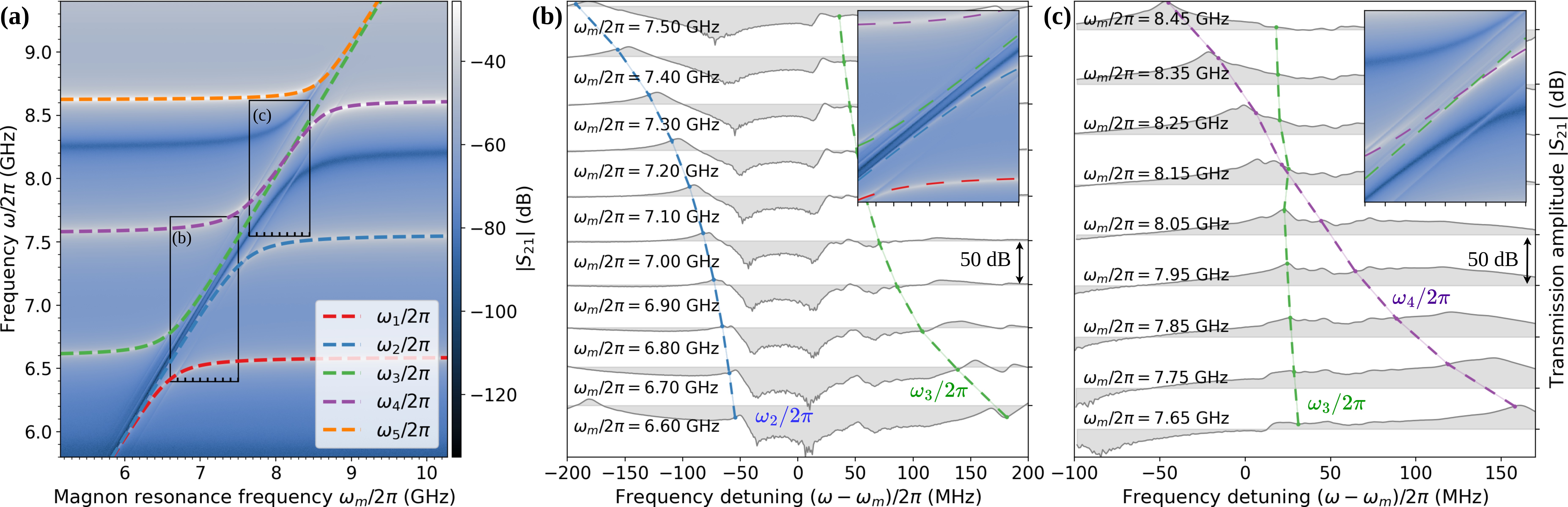
((a))

((b))

((c))

Figure 5: (a) Experimental transmission amplitude ($\absolutevalue{S_{21}}$) of cavity $\pi 0$, with the theoretical spectrum in dashed lines. The two rectangles show the data range used in (b) and (c), with the ticks on the bottom indicating the $\omega_{m}/2\pi$ cuts. (b-c) Transmission amplitude cuts for different $\omega_{m}/2\pi$, with the spectrum in dashed lines. As in fig. 3(b), the average value of the transmission is used to define the horizontal line from which the colouring begins. The fit parameters are indicated in table 2 with the cavity resonances $\omega_{c,1}/2\pi=6.594$ GHz, $\omega_{c,2}/2\pi=7.562$ GHz and $\omega_{c,3}/2\pi=8.619$ GHz. The legend is common to all three subfigures and the curves are all offset by 50 dB.

Compared with cavity $\pi$ we notice the appearance of higher-order magnon modes, which manifests as anti-crossings located away from the magnon resonance $\omega_{m}/2\pi$. The excitation of these higher-order magnonic modes can be explained by the fact that the sphere used in this experiment are bigger (radius of 0.5mm, similar to the radius of the left and right posts, see fig. 4), and thus the cavity modes magnetic fields are less uniform over the spheres. Finally, as shown in appendix B, we also observe the $\sqrt{2}$ enhancement of the frequency gap at the anticrossings due to the coherent coupling of the two distant spin ensembles.

V Conclusion and outlook

To summarise our results, we have proposed to use three-posts re-entrant cavities to engineer the coupling phases, which leads to engineering synthetic gauge fields. The experimental data was shown to match with numerical predictions based on the theory developed in [51]. Depending on the value of the physical phase $\theta$ which parametrises the physics, we observe either a cavity-mediated magnon-magnon coupling ($\theta=\pi$), or dark mode physics ($\theta=0$). These findings are relevant for indirect coupling applications and the creation of non-reciprocal behaviours.

Concerning the former, we verified the $\sqrt{2}$ enhancement of the coupling strength due to having two distant macroscopic spin ensembles coherently coupling with the cavity mode. In the case of $\theta=\pi$, the magnon-magnon coupling extends in the dispersive regime, where both magnons are strongly detuned from the cavity modes. As shown in [51], this results from the constructive interference of the cavity-mediated coupling by both cavity modes (while for $\theta=0$, the cavity-mediated couplings interfere destructively). It was shown that the dispersive regime is advantageous for sensing applications based on magnons (i.e. magnetometry [58] or dark matter detection [59]) so these schemes could benefit from engineering the coupling phases.

This flexibility in the cavity-mediated coupling can also be useful for coupling magnons with superconducting qubits, through the cavity modes. Indeed, transmon qubits couple to the electric field of the cavity modes, which in re-entrant cavities is focused on top of the posts. The existence of several cavity modes, which may or may not couple to the magnons, is thus interesting for developing quantum information processing.

Furthermore, in loop-coupled systems, each loop is associated with a synthetic $U(1)$ gauge field [45]. An interesting application of synthetic gauge fields resides in the creation of non-reciprocal behaviour, which requires breaking time-reversal symmetry and dissipation engineering [45, 49, 50]. Concerning the former, for appropriate values of the physical phase, time-reversal symmetry can be broken [45, 50], and thus in principle this could lead to non-reciprocal behaviour in cavity magnonics system. Here the synthetic gauge field is fixed by the coupling phases, which are themselves fixed by the geometry of the cavity. Nonetheless, tunability could be achieved by modulating the frequencies of one or more magnons [50], for instance by directly driving a YIG sphere using a loop generating a magnetic field parallel to the static magnetic field. Hence, in principle, re-entrant cavities can be used to engineer a loop-coupled system, and by tuning the gauge-invariant phases, either through cavity engineering or driving the YIG spheres, one can create non-reciprocal behaviour in the microwave frequency range.

Appendix A Simulation results

In this appendix, we compare the simulations results of the eigenmode and frequency-domain analyses of COMSOL Multiphysics^®. The eigenmode simulations give the values of the coupling strengths and physical phases, while the frequency-domain simulations give the transmission coefficient $S_{21}$. We use the results of the eigenmode analysis to plot the spectrum on top of the frequency-domain simulations, and we obtain good agreement, as shown in fig. 6 for cavity $\pi$ and fig. 7 for cavity $\pi 0$.

Figure 6: Frequency-domain simulation using COMSOL Multiphysics^® of the transmission through cavity $\pi$. The spectra predicted using the eigenmode analysis of COMSOL is plotted on top, with the eigen-frequencies given in fig. 2 and the other parameters given by table 1.

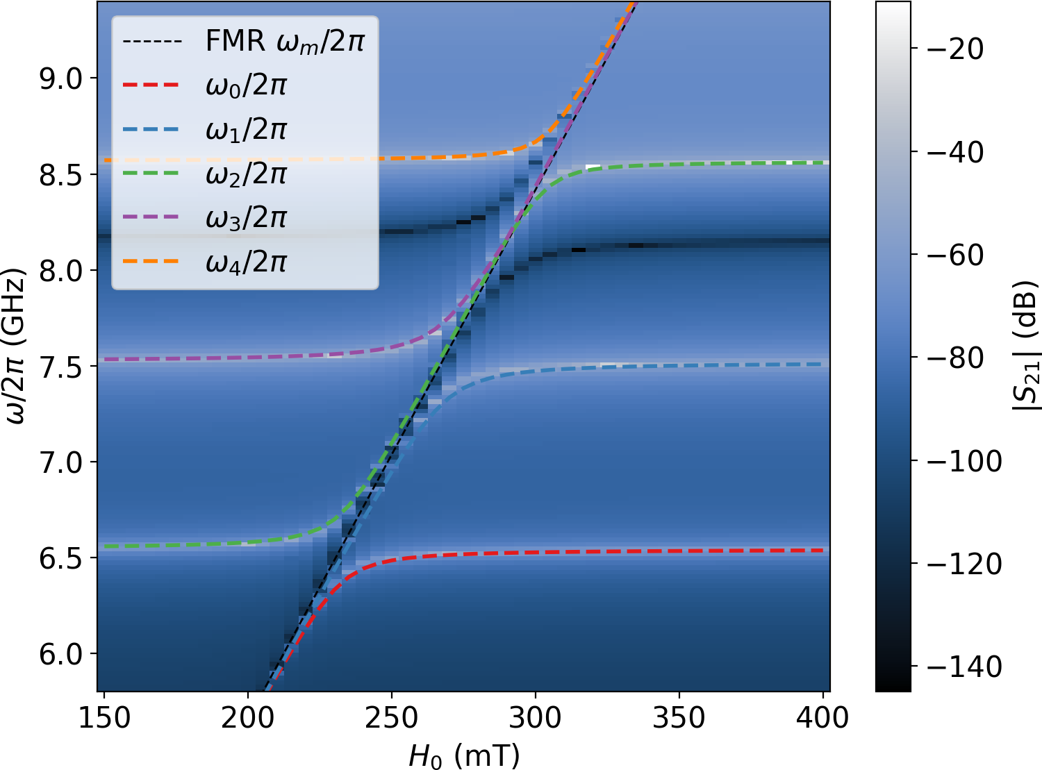
Figure 7: Frequency-domain simulation using COMSOL Multiphysics^® of the transmission through cavity $\pi 0$. The spectra predicted using the eigenmode analysis of COMSOL is plotted on top, with the eigen-frequencies given in section IV of the main text, and other parameters given by table 2.

Appendix B Coherent coupling of two distant spheres

The coherent coupling of $N$ YIG spheres to a cavity mode leads to an enhancement $\sqrt{N}$ of the frequency gap when the magnons are on resonance with the cavity mode [42]. To check that this is indeed the case, we removed one of the YIG spheres and measured again cavity $\pi$ and $\pi 0$. The experimental results are given in fig. 8 for cavity $\pi$ and fig. 9 for cavity $\pi 0$.

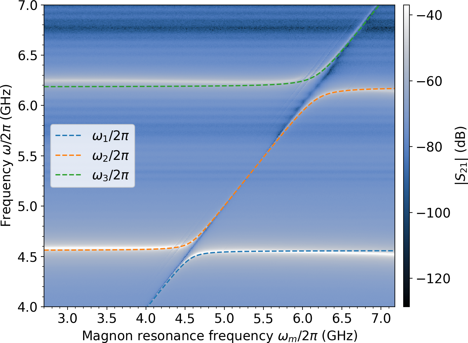
Figure 8: Experimental transmission amplitude ($\absolutevalue{S_{21}}$) of cavity $\pi$ loaded with a single YIG sphere instead of two, with the theoretical spectrum in coloured lines. The fit parameters are identical to those of fig. 3(a), except for a shift of the first cavity mode, set to $\omega_{c,1}/2\pi=4.56$ GHz instead.

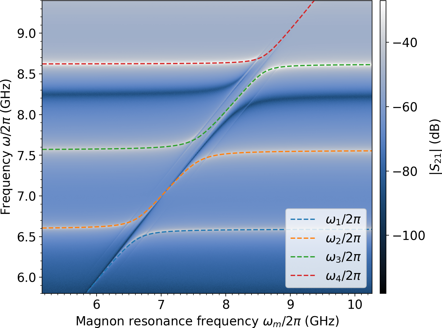
Figure 9: Experimental transmission amplitude ($\absolutevalue{S_{21}}$) of cavity $\pi 0$ loaded with a single YIG sphere instead of two, with the theoretical spectrum in coloured lines. The fit parameters are exactly the same as those in fig. 5.

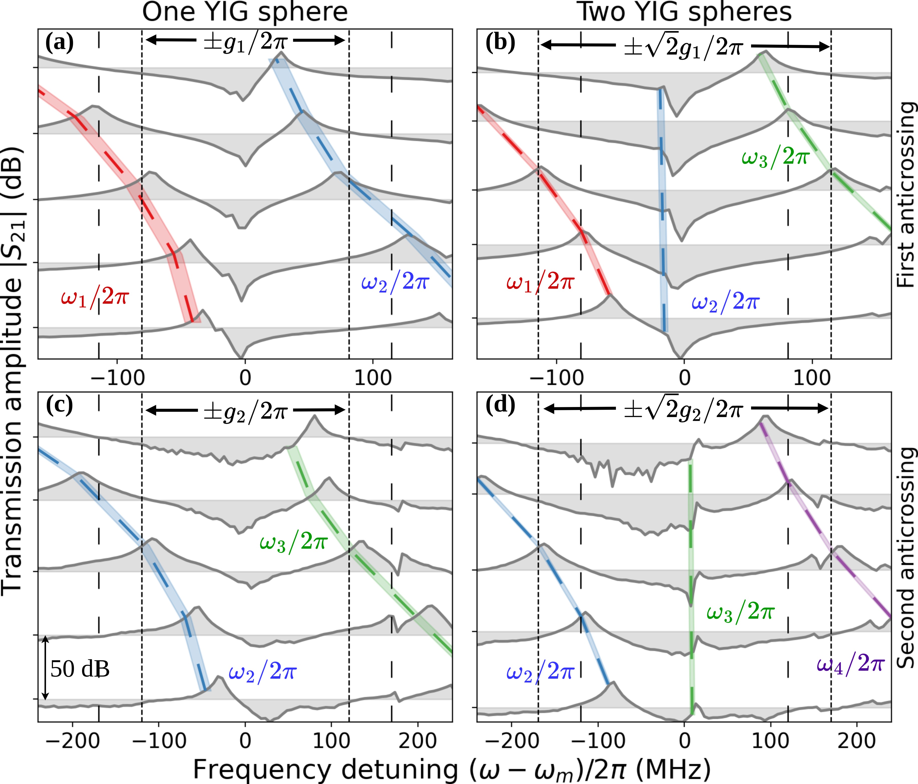
Figure 10: Experimental transmission amplitude $\absolutevalue{S_{21}}$ of cavity $\pi$ for (a-b) the first anticrossing and (c-d) the second anticrossing. In the left column, we show the results for a single YIG sphere present in the cavity, while in the right column we show the case of two YIG spheres. From bottom to top, the line cuts in each subfigure are shown at $\omega_{m}\in\quantity{\omega_{c,k}-2g_{k},\omega_{c,k}-g_{k},\omega_{c,k},\omega_{c,k}+g_{k},\omega_{c,k}+2g_{k}}$. In all the subfigures, the curves are offset by 50 dB.

((a))

((b))

((c))

((d))

In fig. 10(d), we compare the anti-crossings for cavity $\pi$ when a single YIG sphere is loaded in the cavity (figs. 10(a) and 10(c)), versus two YIG spheres (figs. 10(b) and 10(d)). The dashed coloured lines track the polariton frequencies and are seen to follow the resonance peaks. In particular, the third line cut corresponds to the magnon(s) being on resonance with the cavity mode, for which the anticrossing frequency gap is minimum. We see that in the case of a single YIG sphere, this frequency gap is given by $2g_{k}/2\pi$ (first column), while for two YIG spheres the gap is $2\sqrt{2}g_{k}/2\pi$ (second column).

We carried out the same analysis for cavity $\pi 0$ in fig. 11(f), and the the $\sqrt{2}$ enhancement is also verified. In fig. 11(f), the vertical lines indicating $\pm\sqrt{2}g_{3}$ seem to be offset to the left. Note that if a YIG sphere is removed, the system is not loop-coupled anymore, and thus the effects of the coupling phases disappear.

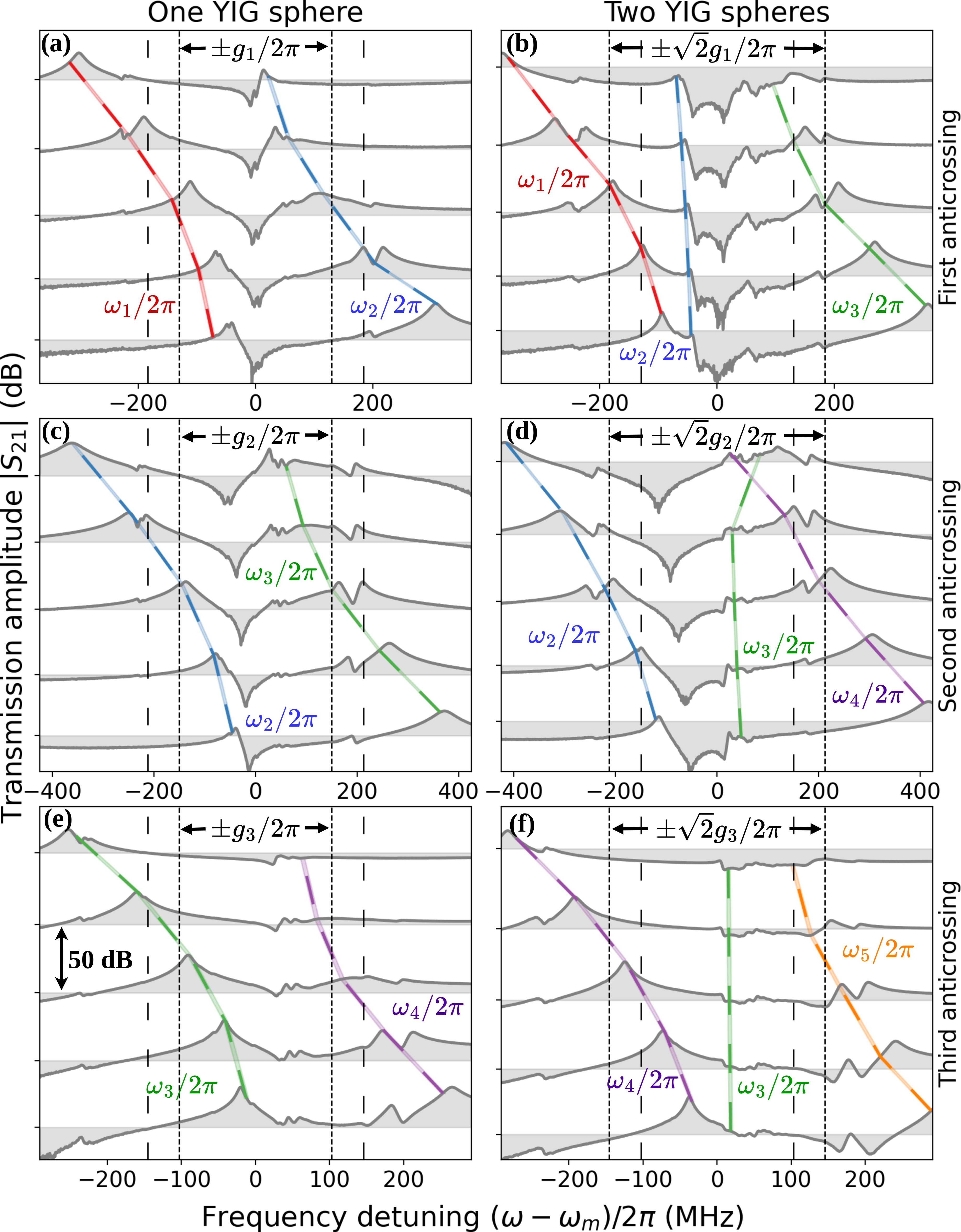
Figure 11: Experimental transmission amplitude $\absolutevalue{S_{21}}$ of cavity $\pi 0$ for (a-b) the first anticrossing, (c-d) the second anticrossing and (e-f) the third anticrossing. In the left column, we show the results for a single YIG sphere present in the cavity, while in the right column we show the case of two YIG spheres. From bottom to top, the line cuts in each subfigure are shown at $\omega_{m}\in\quantity{\omega_{c,k}-2g_{k},\omega_{c,k}-g_{k},\omega_{c,k},\omega_{c,k}+g_{k},\omega_{c,k}+2g_{k}}$. In all the subfigures, the curves are offset by 50 dB.

((a))

((b))

((c))

((d))

((e))

((f))

References

- Wolf et al. [2001] S. A. Wolf, D. D. Awschalom, R. A. Buhrman, J. M. Daughton, S. von Molnar, M. L. Roukes, A. Y. Chtchelkanova, and D. M. Treger, Spintronics: A spin-based electronics vision for the future, Science 294, 1488 (2001).
- Chumak et al. [2015] A. V. Chumak, V. I. Vasyuchka, A. A. Serga, and B. Hillebrands, Magnon spintronics, Nature Physics 11, 453 (2015).
- Csaba et al. [2017] G. Csaba, Á. Papp, and W. Porod, Perspectives of using spin waves for computing and signal processing, Physics Letters A 381, 1471 (2017).
- Chumak et al. [2017] A. V. Chumak, A. A. Serga, and B. Hillebrands, Magnonic crystals for data processing, Journal of Physics D: Applied Physics 50, 244001 (2017).
- Chumak [2019] A. V. Chumak, Fundamentals of magnon-based computing 10.48550/ARXIV.1901.08934 (2019), arXiv:1901.08934 [cond-mat.mes-hall] .
- Barman et al. [2021] A. Barman, G. Gubbiotti, S. Ladak, A. O. Adeyeye, M. Krawczyk, J. Gräfe, C. Adelmann, S. Cotofana, A. Naeemi, V. I. Vasyuchka, B. Hillebrands, S. A. Nikitov, H. Yu, D. Grundler, A. V. Sadovnikov, A. A. Grachev, S. E. Sheshukova, J.-Y. Duquesne, M. Marangolo, G. Csaba, W. Porod, V. E. Demidov, S. Urazhdin, S. O. Demokritov, E. Albisetti, D. Petti, R. Bertacco, H. Schultheiss, V. V. Kruglyak, V. D. Poimanov, S. Sahoo, J. Sinha, H. Yang, M. Münzenberg, T. Moriyama, S. Mizukami, P. Landeros, R. A. Gallardo, G. Carlotti, J.-V. Kim, R. L. Stamps, R. E. Camley, B. Rana, Y. Otani, W. Yu, T. Yu, G. E. W. Bauer, C. Back, G. S. Uhrig, O. V. Dobrovolskiy, B. Budinska, H. Qin, S. van Dijken, A. V. Chumak, A. Khitun, D. E. Nikonov, I. A. Young, B. W. Zingsem, and M. Winklhofer, The 2021 magnonics roadmap, Journal of Physics: Condensed Matter 33, 413001 (2021).
- Mahmoud et al. [2020] A. Mahmoud, F. Ciubotaru, F. Vanderveken, A. V. Chumak, S. Hamdioui, C. Adelmann, and S. Cotofana, Introduction to spin wave computing, Journal of Applied Physics 128, 10.1063/5.0019328 (2020).
- Bhatti et al. [2017] S. Bhatti, R. Sbiaa, A. Hirohata, H. Ohno, S. Fukami, and S. Piramanayagam, Spintronics based random access memory: a review, Materials Today 20, 530 (2017).
- Chumak et al. [2022] A. V. Chumak, P. Kabos, M. Wu, C. Abert, C. Adelmann, A. Adeyeye, J. Åkerman, F. G. Aliev, A. Anane, A. Awad, C. H. Back, A. Barman, G. E. W. Bauer, M. Becherer, E. N. Beginin, V. A. S. V. Bittencourt, Y. M. Blanter, P. Bortolotti, I. Boventer, D. A. Bozhko, S. Bunyaev, J. J. Carmiggelt, R. R. Cheenikundil, F. Ciubotaru, S. Cotofana, G. Csaba, O. Dobrovolskiy, C. Dubs, M. Elyasi, K. G. Fripp, H. Fulara, I. A. Golovchanskiy, C. Gonzalez-Ballestero, P. Graczyk, D. Grundler, P. Gruszecki, G. Gubbiotti, K. Guslienko, A. O. Haldar, S. Hamdioui, R. Hertel, B. Hillebrands, T. Hioki, A. Houshang, C.-M. Hu, H. Huebl, M. Huth, E. N. Iacocca, M. B. Jungfleisch, G. Kakazei, A. Khitun, R. Khymyn, T. Kikkawa, M. Kläui, O. Klein, J. W. Klos, S. Knauer, S. Koraltan, M. Kostylev, M. Krawczyk, I. N. Krivorotov, V. V. Kruglyak, D. Lachance-Quirion, S. Ladak, R. Lebrun, Y. Li, M. Lindner, R. Macêdo, S. Mayr, G. A. Melkov, S. Mieszczak, Y. Nakamura, H. Nembach, A. A. Nikitin, S. A. Nikitov, V. Novosad, J. Otalora, Y. Otani, A. Papp, B. Pigeau, P. Pirro, W. Porod, F. Porrati, H. Qin, B. Rana, T. Reimann, F. Riente, O. Romero-Isart, A. Ross, A. V. Sadovnikov, E. Saitoh, G. Schmidt, H. Schultheiss, K. Schultheiss, A. A. Serga, S. Sharma, J. Shaw, D. Suess, O. Surzhenko, K. Szulc, T. TANIGUCHI, M. Urbánek, K. Usami, A. B. Ustinov, T. Van Der Sar, S. Van Dijken, V. I. Vasyuchka, R. Verba, S. V. Kusminskiy, Q. Wang, M. Weides, M. Weiler, S. Wintz, S. P. Wolski, and X. Zhang, Roadmap on spin-wave computing concepts, (2022), working paper or preprint.
- Grollier et al. [2020] J. Grollier, D. Querlioz, K. Y. Camsari, K. Everschor-Sitte, S. Fukami, and M. D. Stiles, Neuromorphic spintronics, Nature Electronics 3, 360 (2020).
- Harder et al. [2021] M. Harder, B. M. Yao, Y. S. Gui, and C.-M. Hu, Coherent and dissipative cavity magnonics, Journal of Applied Physics 129, 201101 (2021).
- Rameshti et al. [2021] B. Z. Rameshti, S. V. Kusminskiy, J. A. Haigh, K. Usami, D. Lachance-Quirion, Y. Nakamura, C.-M. Hu, H. X. Tang, G. E. Bauer, and Y. M. Blanter, Cavity magnonics (2021), arXiv:2106.09312 [cond-mat.mes-hall] .
- Yuan et al. [2022] H. Yuan, Y. Cao, A. Kamra, R. A. Duine, and P. Yan, Quantum magnonics: When magnon spintronics meets quantum information science, Physics Reports 965, 1 (2022).
- [14] D. Lachance-Quirion, Y. Tabuchi, A. Gloppe, K. Usami, and Y. Nakamura, Hybrid quantum systems based on magnonics, Applied Physics Express 12, 070101.
- Zhang et al. [2016] X. Zhang, C.-L. Zou, L. Jiang, and H. X. Tang, Cavity magnomechanics, Science Advances 2, 10.1126/sciadv.1501286 (2016).
- Tabuchi et al. [2015] Y. Tabuchi, S. Ishino, A. Noguchi, T. Ishikawa, R. Yamazaki, K. Usami, and Y. Nakamura, Coherent coupling between a ferromagnetic magnon and a superconducting qubit, Science 349, 405 (2015).
- [17] Y. Tabuchi, S. Ishino, A. Noguchi, T. Ishikawa, R. Yamazaki, K. Usami, and Y. Nakamura, Quantum magnonics: The magnon meets the superconducting qubit, Comptes Rendus Physique 17, 729, quantum microwaves / Micro-ondes quantiques.
- Lachance-Quirion et al. [2017] D. Lachance-Quirion, Y. Tabuchi, S. Ishino, A. Noguchi, T. Ishikawa, R. Yamazaki, and Y. Nakamura, Resolving quanta of collective spin excitations in a millimeter-sized ferromagnet, Science Advances 3, 10.1126/sciadv.1603150 (2017).
- Lachance-Quirion et al. [2020] D. Lachance-Quirion, S. P. Wolski, Y. Tabuchi, S. Kono, K. Usami, and Y. Nakamura, Entanglement-based single-shot detection of a single magnon with a superconducting qubit, Science 367, 425 (2020).
- Crescini et al. [2021a] N. Crescini, C. Braggio, G. Carugno, A. Ortolan, and G. Ruoso, Coherent coupling between multiple ferrimagnetic spheres and a microwave cavity at millikelvin temperatures, Physical Review B 104, 064426 (2021a).
- [21] N. J. Lambert, J. A. Haigh, S. Langenfeld, A. C. Doherty, and A. J. Ferguson, Cavity-mediated coherent coupling of magnetic moments, Physical Review A 93, 021803.
- Hyde et al. [2016] P. Hyde, L. Bai, M. Harder, C. Match, and C.-M. Hu, Indirect coupling between two cavity modes via ferromagnetic resonance, Applied Physics Letters 109, 152405 (2016).
- Goryachev et al. [2014] M. Goryachev, W. G. Farr, D. L. Creedon, Y. Fan, M. Kostylev, and M. E. Tobar, High-cooperativity cavity qed with magnons at microwave frequencies, Phys. Rev. Applied 2, 054002 (2014).
- Kostylev et al. [2016] N. Kostylev, M. Goryachev, and M. E. Tobar, Superstrong coupling of a microwave cavity to yttrium iron garnet magnons, Applied Physics Letters 108, 062402 (2016).
- Golovchanskiy et al. [2021a] I. Golovchanskiy, N. Abramov, V. Stolyarov, A. Golubov, M. Y. Kupriyanov, V. Ryazanov, and A. Ustinov, Approaching deep-strong on-chip photon-to-magnon coupling, Phys. Rev. Applied 16, 034029 (2021a).
- Golovchanskiy et al. [2021b] I. A. Golovchanskiy, N. N. Abramov, V. S. Stolyarov, M. Weides, V. V. Ryazanov, A. A. Golubov, A. V. Ustinov, and M. Y. Kupriyanov, Ultrastrong photon-to-magnon coupling in multilayered heterostructures involving superconducting coherence via ferromagnetic layers, Science Advances 7, 10.1126/sciadv.abe8638 (2021b).
- Bourcin et al. [2022] G. Bourcin, J. Bourhill, V. Vlaminck, and V. Castel, Strong to ultra-strong coherent coupling measurements in a yig/cavity system at room temperature, (2022), arXiv:2209.14643 [quant-ph] .
- Yu et al. [2019] W. Yu, J. Wang, H. Yuan, and J. Xiao, Prediction of attractive level crossing via a dissipative mode, Physical Review Letters 123, 227201 (2019).
- Zhao et al. [2020] J. Zhao, Y. Liu, L. Wu, C.-K. Duan, Y.-x. Liu, and J. Du, Observation of anti-pt-symmetry phase transition in the magnon-cavity-magnon coupled system, Physical Review Applied 13, 014053 (2020).
- Harder et al. [2018] M. Harder, Y. Yang, B. Yao, C. Yu, J. Rao, Y. Gui, R. Stamps, and C.-M. Hu, Level attraction due to dissipative magnon-photon coupling, Physical Review Letters 121, 137203 (2018).
- Bhoi et al. [2019] B. Bhoi, B. Kim, S.-H. Jang, J. Kim, J. Yang, Y.-J. Cho, and S.-K. Kim, Abnormal anticrossing effect in photon-magnon coupling, Physical Review B 99, 134426 (2019).
- Yang et al. [2019] Y. Yang, J. Rao, Y. Gui, B. Yao, W. Lu, and C.-M. Hu, Control of the magnon-photon level attraction in a planar cavity, Physical Review Applied 11, 054023 (2019).
- Yao et al. [2019a] B. Yao, T. Yu, X. Zhang, W. Lu, Y. Gui, C.-M. Hu, and Y. M. Blanter, The microscopic origin of magnon-photon level attraction by traveling waves: Theory and experiment, Physical Review B 100, 214426 (2019a).
- Yao et al. [2019b] B. Yao, T. Yu, Y. S. Gui, J. W. Rao, Y. T. Zhao, W. Lu, and C.-M. Hu, Coherent control of magnon radiative damping with local photon states, Communications Physics 2, 10.1038/s42005-019-0264-z (2019b).
- Lu et al. [2021] Z. Lu, X. Mi, Q. Zhang, Y. Sun, J. Guo, Y. Tian, S. Yan, and L. Bai, Interference induced microwave transmission in the YIG-microstrip cavity system, Journal of Magnetism and Magnetic Materials 540, 168457 (2021).
- Wang et al. [2019] Y.-P. Wang, J. Rao, Y. Yang, P.-C. Xu, Y. Gui, B. Yao, J. You, and C.-M. Hu, Nonreciprocity and unidirectional invisibility in cavity magnonics, Physical Review Letters 123, 127202 (2019).
- Kong et al. [2022] C. Kong, J. Liu, and H. Xiong, Nonreciprocal microwave transmission under the joint mechanism of phase modulation and magnon kerr nonlinearity effect, Frontiers of Physics 18, 10.1007/s11467-022-1203-0 (2022).
- Li et al. [2022] X. Li, J. Li, X. Cheng, and G. an Li, Nonreciprocal transmission in a four-mode cavity magnonics system, Laser Physics Letters 19, 095208 (2022).
- Zhu et al. [2020] N. Zhu, X. Han, C.-L. Zou, M. Xu, and H. X. Tang, Magnon-photon strong coupling for tunable microwave circulators, Physical Review A 101, 043842 (2020).
- Boventer et al. [2019] I. Boventer, M. Kläui, R. Macêdo, and M. Weides, Steering between level repulsion and attraction: broad tunability of two-port driven cavity magnon-polaritons, New Journal of Physics 21, 125001 (2019).
- Boventer et al. [2020] I. Boventer, C. Dörflinger, T. Wolz, R. Macêdo, R. Lebrun, M. Kläui, and M. Weides, Control of the coupling strength and linewidth of a cavity magnon-polariton, Physical Review Research 2, 013154 (2020).
- [42] X. Zhang, C.-L. Zou, N. Zhu, F. Marquardt, L. Jiang, and H. X. Tang, Magnon dark modes and gradient memory, Nature Communications 6, 10.1038/ncomms9914.
- Zheng et al. [2019] S. Zheng, F. Sun, Y. Lai, Q. Gong, and Q. He, Manipulation and enhancement of asymmetric steering via interference effects induced by closed-loop coupling, Physical Review A 99, 022335 (2019).
- Huang et al. [2023] J. Huang, D.-G. Lai, and J.-Q. Liao, Controllable generation of mechanical quadrature squeezing via dark-mode engineering in cavity optomechanics, Physical Review A 108, 013516 (2023), arXiv:2304.00963 [quant-ph] .
- Koch et al. [2010] J. Koch, A. A. Houck, K. L. Hur, and S. M. Girvin, Time-reversal-symmetry breaking in circuit-QED-based photon lattices, Physical Review A 82, 043811 (2010).
- Bernier et al. [2017] N. R. Bernier, L. D. Tóth, A. Koottandavida, M. A. Ioannou, D. Malz, A. Nunnenkamp, A. K. Feofanov, and T. J. Kippenberg, Nonreciprocal reconfigurable microwave optomechanical circuit, Nature Communications 8, 10.1038/s41467-017-00447-1 (2017).
- Fang et al. [2017] K. Fang, J. Luo, A. Metelmann, M. H. Matheny, F. Marquardt, A. A. Clerk, and O. Painter, Generalized non-reciprocity in an optomechanical circuit via synthetic magnetism and reservoir engineering, Nature Physics 13, 465 (2017).
- Chen et al. [2021] Y. Chen, Y.-L. Zhang, Z. Shen, C.-L. Zou, G.-C. Guo, and C.-H. Dong, Synthetic gauge fields in a single optomechanical resonator, Physical Review Letters 126, 123603 (2021).
- Metelmann and Clerk [2015] A. Metelmann and A. A. Clerk, Nonreciprocal photon transmission and amplification via reservoir engineering, Physical Review X 5, 021025 (2015).
- Clerk [2022] A. Clerk, Introduction to quantum non-reciprocal interactions: from non-hermitian hamiltonians to quantum master equations and quantum feedforward schemes, SciPost Physics Lecture Notes 10.21468/scipostphyslectnotes.44 (2022).
- Gardin et al. [2023] A. Gardin, J. Bourhill, V. Vlaminck, C. Person, C. Fumeaux, V. Castel, and G. C. Tettamanzi, Manifestation of the coupling phase in microwave cavity magnonics, Physical Review Applied 19, 054069 (2023), arXiv:2212.05389 [quant-ph] .
- Holstein and Primakoff [1940] T. Holstein and H. Primakoff, Field dependence of the intrinsic domain magnetization of a ferromagnet, Phys. Rev. 58, 1098 (1940).
- [53] G. Flower, M. Goryachev, J. Bourhill, and M. E. Tobar, Experimental implementations of cavity-magnon systems: from ultra strong coupling to applications in precision measurement, New Journal of Physics 21, 095004.
- [54] J. Bourhill, V. Castel, A. Manchec, and G. Cochet, Universal characterization of cavity–magnon polariton coupling strength verified in modifiable microwave cavity, Journal of Applied Physics 128, 073904.
- Frisk Kockum et al. [2019] A. Frisk Kockum, A. Miranowicz, S. De Liberato, S. Savasta, and F. Nori, Ultrastrong coupling between light and matter, Nature Reviews Physics 1, 19–40 (2019).
- Le Boité [2020] A. Le Boité, Theoretical methods for ultrastrong light–matter interactions, Advanced Quantum Technologies 3, 1900140 (2020), https://onlinelibrary.wiley.com/doi/pdf/10.1002/qute.201900140 .
- Nair et al. [2022] J. M. P. Nair, D. Mukhopadhyay, and G. S. Agarwal, Cavity-mediated level attraction and repulsion between magnons, Physical Review B 105, 214418 (2022).
- Crescini et al. [2021b] N. Crescini, G. Carugno, and G. Ruoso, Phase-modulated cavity magnon polaritons as a precise magnetic field probe, Physical Review Applied 16, 034036 (2021b).
- Flower et al. [2019] G. Flower, J. Bourhill, M. Goryachev, and M. E. Tobar, Broadening frequency range of a ferromagnetic axion haloscope with strongly coupled cavity–magnon polaritons, Physics of the Dark Universe 25, 100306 (2019).
- Crameri [2021] F. Crameri, Scientific colour maps (2021).
- Crameri et al. [2020] F. Crameri, G. E. Shephard, and P. J. Heron, The misuse of colour in science communication, Nature Communications 11, 10.1038/s41467-020-19160-7 (2020).