JWST detection of extremely excited outflowing CO and H₂O in VV 114 E SW: a possible rapidly accreting IMBH

Mid-infrared (mid-IR) gas-phase molecular bands are powerful diagnostics of the warm interstellar medium. We report the James Webb Space Telescope detection of the CO $v=1-0$ ($4.4-5.0$ $\mu$m) and H₂O $\nu_{2}=1-0$ ($5.0-7.8$ $\mu$m) ro-vibrational bands, both in absorption, toward the “s2” core in the southwest nucleus of the merging galaxy VV 114 E. All ro-vibrational CO lines up to $J_{\mathrm{low}}=33$ ($E_{\mathrm{low}}\approx 3000$ K) are detected, as well as a forest of H₂O lines up to $13_{0,13}$ ($E_{\mathrm{low}}\approx 2600$ K). The highest-excitation lines are blueshifted by $\sim 180$ km s^-1 relative to the extended molecular cloud, which is traced by the rotational CO ($J=3-2$) 346 GHz line observed with the Atacama Large Millimeter/submillimeter Array. The bands also show absorption in a low-velocity component (blueshifted by $\approx 30$ km s^-1) with lower excitation. The analysis shows that the bands are observed against a continuum with effective temperature of $T_{\mathrm{bck}}\sim 550$ K extinguished with $\tau_{\mathrm{6\mu m}}^{\mathrm{ext}}\sim 2.5-3$ ($A_{k}\sim 6.9-8.3$ mag). The high-excitation CO and H₂O lines are consistent with $v=0$ thermalization with $T_{\mathrm{rot}}\approx 450$ K and column densities of $N_{\mathrm{CO}}\approx(1.7-3.5)\times 10^{19}$ cm^-2 and $N_{\mathrm{H_{2}O}}\approx(1.5-3.0)\times 10^{19}$ cm^-2. Thermalization of the $v=0$ levels of H₂O requires either an extreme density of $n_{\mathrm{H_{2}}}\gtrsim 10^{9}$ cm^-3, or radiative excitation by the mid-IR field in a very compact ($<1$ pc) optically thick source emitting $\sim 10^{10}\,L_{\odot}$. The latter alternative is favored, implying that the observed absorption probes the very early stages of a fully enshrouded active black hole (BH). On the basis of a simple model for BH growth and applying a lifetime constraint to the s2 core, an intermediate-mass BH (IMBH, $M_{\mathrm{BH}}\sim 4.5\times 10^{4}\,M_{\odot}$) accreting at super-Eddington rates is suggested, where the observed feedback has not yet been able to break through the natal cocoon.

1 Introduction

Major galaxy mergers leading to (ultra-)luminous infrared galaxies ((U)LIRGs) are considered important precursors for the formation and growth of super massive black holes (SMBHs, $>10^{6}\,M_{\odot}$) in the local universe (Sanders & Mirabel, 1996). While the general process, involving tidal forces that efficiently funnel gas towards the galactic center(s) (e.g., Hopkins et al., 2006), is well constrained observationally, the earliest phases of intermediate-mass black hole (IMBH, $\sim 10^{2-5}\,M_{\odot}$) formation and growth in mergers are unconstrained (see recent reviews by Greene et al., 2020; Askar et al., 2023). Close to the high end of the IMBH mass range, the (so far) few identifications have been based on dynamical measurements in nearby, mostly dwarf galaxies ($\lesssim 10$ Mpc; e.g., Nguyen et al., 2019; Herrnstein et al., 2005; Pechetti et al., 2022), and beyond the Local Group from optical spectroscopy (i.e., the broad and narrow line regions, Baldassare et al., 2015), X-ray emission (Davis et al., 2011), and tidal disruption events (TDEs, Lin et al., 2018). At the lower end, detections come from gravitational wave events (Abbott et al., 2020). Potential tracers are also radio emission, mid-infrared (mid-IR) colors, polycyclic aromatic hydrocarbons (PAHs), and spectroscopy of high ionization potential ions (e.g., Greene et al., 2020, and references therein). However, some of these measurements are challenging due to low-level emission and potential confusion with stellar activity (Casares & Jonker, 2015; Greene et al., 2020; Askar et al., 2023).

To date, there have been no reported detections of IMBHs in (U)LIRG mergers. In wet mergers, some of the above diagnostics are critical at early stages of IMBH growth when high amounts of gas and dust may shrink the highly ionized regions (Toyouchi et al., 2021) and obscure the most well known tracers of active galactic nuclei (AGN). Nevertheless, with large reservoirs of gas available, an IMBH may be accreting at super- or even hyper-Eddington rates such that mid-IR observations can trace the surrounding hot dust (e.g., Inayoshi et al., 2016). To identify these high concentrations of hot dust, mid-IR spectroscopy of absorption bands of gas-phase molecular species, namely CO and H₂O, are essential probes.

The gas-phase CO $v=1-0$ 4.7 $\mu$m and H₂O $\nu_{2}=1-0$ 6.3 $\mu$m fundamental bands are powerful mid-IR diagnostics of the interestellar medium (ISM): they probe the physical conditions and gas kinematics by sampling all rotational levels of the ground vibrational state that are significantly populated, and trace the chemistry of the gas via the [CO]/[H₂O] abundance ratio. Since the bands are excited by the mid-IR radiation field, they can also give clues on the ISM geometry relative to the mid-IR luminosity sources in the region, depending on whether the bands are detected in emission, in absorption, or some lines in absorption (within the R-branch) and some in emission (the P-branch). In addition, the relative strength of the ro-vibrational lines can potentially give clues on the gas column density, and on the slope of the exciting continuum emitted by hot dust –and thus on its effective temperature. Previous studies of the CO band in extragalactic sources have been carried out with high spectral resolution using ground-based facilities (Geballe et al., 2006; Shirahata et al., 2013; Onishi et al., 2021), and with low spectral resolution using Spitzer and AKARI (Spoon et al., 2004; Baba et al., 2018). The unprecedented sensitivity of the James Webb Space Telescope (JWST) with the high spectral and spatial resolution provided by the Near-Infrared Spectrograph (NIRSpec, Jakobsen et al., 2022; Böker et al., 2022) and the Mid-Infrared Instrument/Medium-resolution spectroscopy (MIRI/MRS, Rieke et al., 2015; Wright et al., 2015) is ideal to further extend the study of the molecular bands in galaxies (Pereira-Santaella et al., 2023; García-Bernete et al., 2023). We take all spectroscopic parameters for CO and H₂O from the HITRAN2020 database (Gordon et al., 2022).

Here we report and analyze the detection of extremely excited CO and H₂O, observed in absorption, in the local merger VV 114 (IC 1623, IRAS F01053$-$1746), a luminous infrared (LIRG, $L_{\mathrm{IR}}=5\times 10^{11}$ $L_{\odot}$) mid-stage merger (Armus et al., 2009) with the two galaxy components separated by $\sim 6$ kpc. While the western galaxy is bright in the UV (Goldader et al., 2002) and optical (Knop et al., 1994) showing low visual extinction, a large concentration of dust obscures the eastern component (VV 114 E), which dominates the mid-IR emission. VV 114 E has been imaged in several molecular lines at millimeter wavelengths (e.g. Iono et al., 2013; Saito et al., 2015, 2017), showing enhanced emission along a narrow, 4 kpc-long dense filament in the east-west direction (including an overlap region between the two galaxies, see also Fig. 1a,b), in which Pa$\alpha$ emission indicates ongoing star formation (Tateuchi et al., 2012; Iono et al., 2013). This filament, which is resolved into dense clumps of several $\times 10^{6}$ $M_{\odot}$, suggests widespread shocks triggered by the dynamic interaction of the merging disk galaxies. The nucleus of VV 114 E is located at the easternmost extreme edge of the filament, and is also resolved into several massive clumps. JWST/MIRI photometry of up to 40 star-forming knots has been reported by Evans et al. (2022). The possible presence of an AGN in VV 114 E has been debated for years. Analysis of X-ray emission from VV 114 E has not yielded conclusive results on the nature of the source, which has a spectrum harder than other Chandra-detected point sources in the galaxy (Grimes et al., 2006; Garofali et al., 2020). Saito et al. (2015) favor an AGN at the NE core based on the HCN/HCO⁺ ratio. Based on the PAH emission, Donnan et al. (2023) identified a deeply obscured nucleus at NE that could extinguish the undetected coronal lines. On the other hand, Evans et al. (2022) and Rich et al. (2023) proposed that the AGN is located at the SW-s1 clump (see Fig 1e) based on the low PAH equivalent widths and mid- and near-IR colors. To complicate things, the extreme source of CO and H₂O excitation reported here is however located at the SW-s2 knot. We adopt a distance to VV 114 of 88 Mpc.

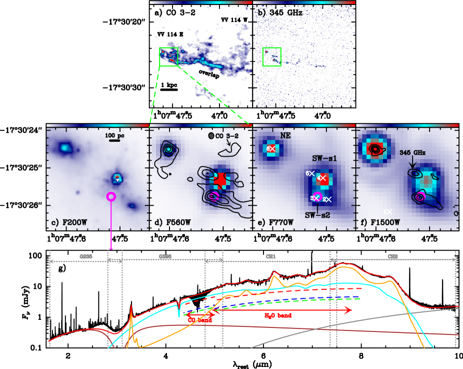
Figure 1: a and b: ALMA maps of CO ($3-2$) (moment 0) and the 345 GHz continuum of the VV 114 system as observed with ALMA. The green box in both panels indicates the nuclear region of VV 114 E mapped in the middle panels. c-f: JWST NIRCam F200W, MIRI F560W, F770W, and F1500 images of the VV 114 E nucleus. Overlaid in panels d and f are the contours of CO ($3-2$) and 345 GHz continuum, respectively. The ALMA beam ($0.16^{\prime\prime}\times 0.14^{\prime\prime}$) is shown in panel d. The 33 GHz continuum sources (Song et al., 2022) are indicated with crosses and labelled in panel e, where we also label the main mid-IR peaks (NE, SW-s1, and SW-s2). The magenta circle, coincident with SW-s2 and 33 GHz source #3, indicates the position where the extreme excitation of CO and H₂O is found. g: The near- and mid-IR spectrum extracted from SW-s2. The extent of the CO and H₂O bands, and of the NIRSpec gratings and MIRI/MRS channels, are indicated. The solid curves show a model for the continuum, including the PAHs (orange) and three blackbody sources with temperatures 1360 (brown), 550 (light-blue), and 230 K (gray); red is total. The light-blue component, dominating the continuum associated with the molecular bands, is attenuated by foreground material with $\tau_{\mathrm{6\mu m}}^{\mathrm{ext}}=2.5$ (see text). The dashed lines indicate the continuum covered by CO and H₂O in the hot ($H_{C}$, in blue), the warm ($W_{C}$, in green), and the sum of both (in red), as predicted by the fiducial model for the bands.

2 Observations and results

We have used the MIRI (imaging and MRS), NIRCam, and NIRSpec IFU data on VV 114 from the Director’s Discretionary Early Release Science (DD-ERS) Program #1328 (PI: L. Armus and A. Evans). The observations and data reduction are described in Appendix A. The images of the VV 114 E nucleus in the NIRCam F200W ($1.7-2.2$ $\mu$m), and MIRI F560W, F770W, and F1500W ($5.0-6.2$, $6.6-8.7$, and $13.5-16.6$ $\mu$m) filters are shown in Fig. 1c-f.

We have also retrieved archival Atacama Large Millimeter/submillimeter Array (ALMA) observations of CO ($J=3-2$) and its associated 345 GHz continuum from program 2013.1.00740.S (PI: T. Saito). The images of the continuum-subtracted CO ($3-2$) emission (moment 0) and 345 GHz continuum (extracted from line-free channels) are shown in Fig. 1a-b (see also Saito et al., 2015). Both maps clearly delineate the elongated filament and peak at the nuclear region of VV 114 E. The IR images of this nucleus, enlarged in Fig. 1c-f, show three main clumps, which will be denoted as NE, SW-s1, and SW-s2 (panel e). These correspond to sources “a”, “c”, and “d” in Rich et al. (2023), and have 33 GHz counterparts “n6”, “n4”, and “n3” as denoted in Song et al. (2022), respectively. The strongest source at 2.0, 5.6, and 7.7 $\mu$m, the latter dominated by PAH emission, is SW-s1, but NE dominates at longer wavelengths (Fig. 1f). It is also worth noting that SW-s1 is devoid of CO ($3-2$) and 345 GHz continuum, which surround the clump (Fig. 1d,f) and peak at NE and SW-s2, which also display the strongest emission at 33 GHz (Song et al., 2022).

We found a source of unusual CO and H₂O excitation in the SW-s2 core, located just at the head of the 4 kpc filament (magenta circle in Fig. 1c-f). The JWST $2-10\,\mu$m spectrum extracted from a $0.2^{\prime\prime}$ aperture at the position of the maximum band strength is shown in Fig. 1g, where the spectral extent of the CO and H₂O bands is indicated.

2.1 The CO $v=1-0$ band

The top panel of Fig. 2 shows the ¹²CO (hereafter CO) $v=1-0$ band of SW-s2 extracted from the NIRSpec high resolution ($\Delta v\sim 90$ km s^-1) grating G395H in Fig. 1g. The baseline used to subtract the continuum is shown and discussed in Appendix B. Absorption is observed in the P-branch up to $J=33$ (lower-level energy of $E_{\mathrm{low}}=3000$ K; the spectral features nearly coincident with P(34) and P(35) are due to H₂O lines). Apparent emission lines in the spectrum are due to H₂ $v=0-0$ S(8), S(9), and S(10), and H I 7-5. The presence of two additional emission lines is inferred from the relatively low absorption in the R(5) and R(24) lines, and are attributed to [K iii] 4.617 $\mu$m and [Mg iv] 4.488 $\mu$m, respectively (Pereira-Santaella et al., 2023; García-Bernete et al., 2023).

As illustrated in the inserts of Fig. 2(upper), the CO ro-vibrational lines are spectrally resolved and much broader (full width at half maximum of $\mathrm{FWHM}=200-270$ km s^-1) than and blueshifted relative to the rotational CO ($3-2$) profile ($\mathrm{FWHM}=105$ km s^-1) extracted from a similar aperture (radius $r=0.162^{\prime\prime}$). Hereafter, we use the redshift of the bulk of the gas in SW-s2, $z=0.02013$, derived from the CO ($3-2$) line fit. Since adjacent R(J) lines are separated by $<520$ km s^-1 (decreasing to $<400$ km s^-1 for $J>22$), they partially overlap forming a pseudo-continuum. Along the P-branch, the CO line velocity separation increases (from 540 to 740 km s^-1), but significant absorption is still seen between adjacent P(6)-P(9), P(13)-P(15), and P(20)-P(21) lines. At these wavelengths the ¹³CO and C¹⁸O ro-vibrational lines lie in between the ¹²CO lines, and thus this absorption is attributed to the rare isotopologues.

A fuller view of the velocity profiles is given in Fig. 3left, which shows an energy level-velocity diagram for the P-branch lines. Up to $J=16$ ($E_{\mathrm{low}}=750$ K) the peak absorption is blueshifted by $70-100$ km s^-1, but the blueshift increases to $\approx 170$ km s^-1 for $J>20$. This is also illustrated by the CO P(25) profile in Fig. 3center, which shows little absorption at central velocities. The data thus indicate the presence of two blueshifted components, with the most excited component (denoted as the hot component, $H_{C}$) more blueshifted than the less excited one (the warm component, $W_{C}$). In addition, strong absorption is seen in the $J\leq 3$ lines ($E_{\mathrm{low}}\leq 33$ K) relative to $J=4$ (Fig. 2upper), indicating the contribution to the absorption by a cold component ($C_{C}$), presumably the quiescent gas that accounts for the CO ($3-2$) emission. The bulk of the absorption in the band is due to the blueshifted $H_{C}$ and $W_{C}$, and therefore the lines are all blueshifted relative to the transition labels in Fig. 2(upper).

To compare the fluxes of the P(J) and R(J) lines arising from the same $J$-level of the $v=0$ state, and due to line blending and contamination by ¹³CO, we use instead the observed peak absorption as shown in Fig. 4a,b. The P-R asymmetry (e.g. González-Alfonso et al., 2002; Pereira-Santaella et al., 2023; García-Bernete et al., 2023) is evaluated from the ratios of the peak absorption (in mJy) of these pairs of lines, showing two different trends: for $J<10$, $\mathrm{P(J)/R(J)}\lesssim 1$, and for $J\geq 10$, $\mathrm{P(J)/R(J)}>1$ increasing up to $\gtrsim 1.5$ for the highest $J$. The latter dependence is expected for a background continuum that rises with $\lambda$, as the P(J) (R(J)) transitions have progressively longer (shorter) wavelengths. A positive slope is indeed observed in the continuum beween $4.4-5.0$ $\mu$m (Fig. 1g), which is matched with a blackbody radiation temperature of $T_{\mathrm{rad}}=390$ K (Appendix B). The $\mathrm{P(J)/R(J)}\lesssim 1$ values found for relatively low $J$ require a mechanism that favors emission in the P-branch at the expense of the R-branch, pointing toward line re-emission from the flanks of the continuum source. CO absorption in the R-branch and emission in the P-branch has been observed toward the disk of NGC 3256-S (Pereira-Santaella et al., 2023) and previously toward the galactic Orion BN/KL (González-Alfonso et al., 1998). No re-emision is however apparent in the $H_{C}$.

Emission lines of other species in the spectrum of SW-s2 do not trace the $H_{C}$. This is illustrated in Fig. 3center, which compares the CO P(25) line profile with those of two H₂ lines, an H recombination line, and the [Fe ii]5.3 $\mu$m one. All emission lines peak at central velocities, with no blueshifted spectral feature similar to the CO P(25) line shape. The CO ($3-2$) line neither shows blueshifted emission, but a line wing at redshifted velocities. A 3-components Gaussian fit to the CO ($3-2$) profile, fixing the central velocity of one component at $-160$ km s^-1 (blue line in the CO ($3-2$) panel of Fig. 3center), establishes an upper limit for the flux of the $H_{C}$ in CO ($3-2$) of $<0.35$ Jy km s^-1, equivalent to a luminosity of $<7.4\times 10^{5}$ K km s^-1 pc² and a gas mass of $M_{\mathrm{gas}}(H_{C})<4.4\times 10^{5}\,M_{\odot}$ (using $\alpha_{\mathrm{CO3-2}}\approx 0.6\,M_{\odot}/(\mathrm{K\,km\,s^{-1}\,pc^{2}})$, Pereira-Santaella et al., 2023). The central velocity component has a CO ($3-2$) flux of $(17.4\pm 0.1)$  Jy km s^-1, which translates into $M_{\mathrm{gas}}(\mathrm{SW-s2})\sim 3\times 10^{7}\,M_{\odot}$ (using $\alpha_{\mathrm{CO3-2}}\approx 0.8\,M_{\odot}/(\mathrm{K\,km\,s^{-1}\,pc^{2}})$) and a beam-averaged column density of $N_{\mathrm{H_{2}}}(\mathrm{SW-s2})\sim 1\times 10^{23}$ cm^-2 ($\Sigma_{\mathrm{gas}}(\mathrm{SW-s2})\sim 2\times 10^{3}$ $M_{\odot}$ pc^-2).

2.2 The H₂O $\nu_{2}=1-0$ band

The striking 5-8 $\mu$m spectral region of SW-s2 (Fig. 2b,c) contains $\sim 150$ spectral features in absorption attributable to the H₂O $\nu_{2}=1-0$ band. Line identification, which is based on the models described below (Sect. 3), indicates that many of these feaures are produced by several blended lines, and we estimate that $\sim 280$ transitions of H₂O significantly contribute to the observed spectrum. As shown in the energy level diagram of Fig. 8, 93 levels of the ground vibrational state up to $13_{0,13}$ ($E_{\mathrm{low}}\approx 2600$ K) are involved.

The H₂O lines also show a blueshift relative to CO ($3-2$), as illustrated with five line profiles in Fig. 3right. As in the case of CO, the low-excitation lines (such as the ground-state $\nu_{2}=1-0$ $1_{10}-1_{01}$ and the $3_{21}-2_{12}$ transitions) are blueshifted by only $50-100$ km s^-1 including significant absorption at central velocities, while higher excitation lines display blueshifts of $\gtrsim 150$ km s^-1. This is similar to the 2 blueshifted velocity components, $W_{C}$ and $H_{C}$, that also dominate the CO band.

To help characterize the complex H₂O band, we show in Fig. 9 the spectrum plotting $E_{\mathrm{low}}$ for the transitions that, according to our models, significantly contribute to the forest of absorption features. Most of the strongest spectral features ($<-2$ mJy, in red) are dominated by low-excitation lines ($E_{\mathrm{low}}\lesssim 500$ K), but some high-excitation transitions ($E_{\mathrm{low}}\gtrsim 800$ K) also generate strong absorption (see details in Appendix C).

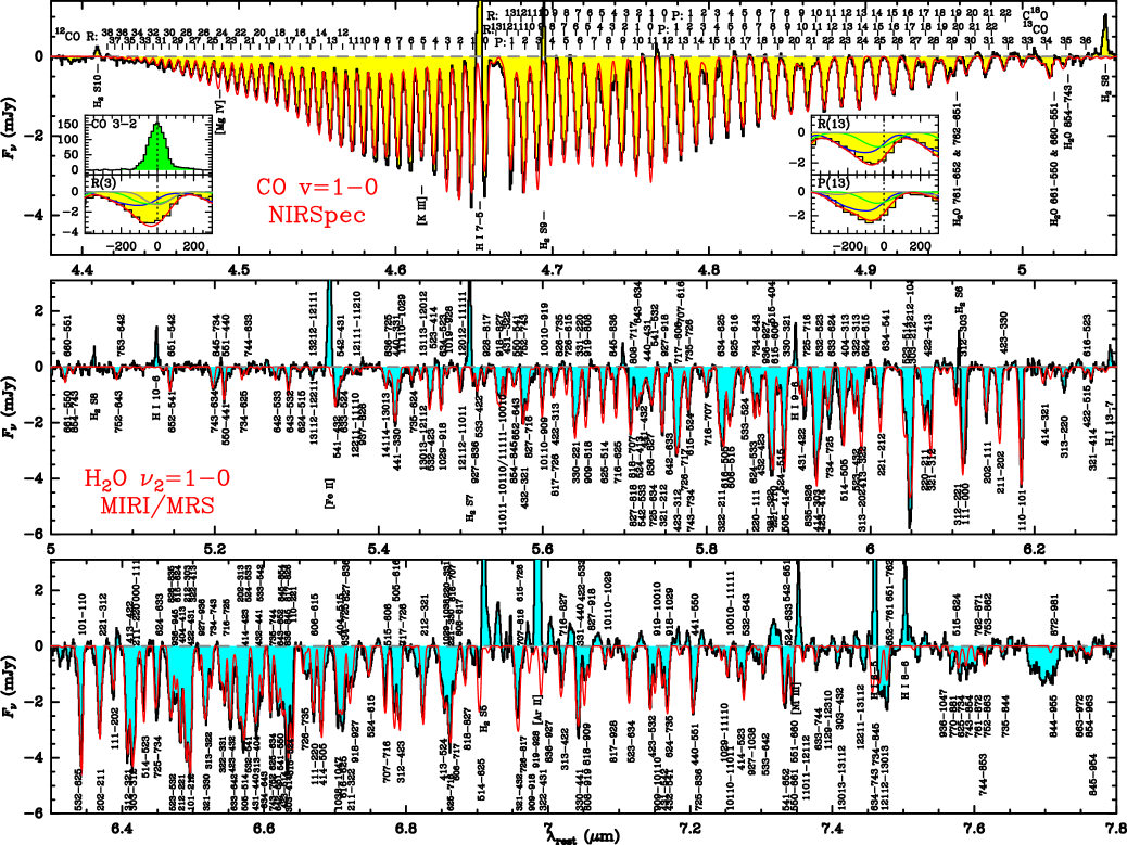
Figure 2: CO $v=1-0$ (upper panel) and H₂O $\nu_{2}=1-0$ (middle and lower) bands in VV 114 SW-s2. Color-filled black histograms show the data, and the red lines show the total absorption predicted by our composite model. The inserts in the upper panel show the spectra of the CO 3-2 line observed with ALMA and several CO $v=1-0$ lines with the abscissae in units of velocity; the contributions of each of the three components (blue: hot; green: warm; gray: cold) are also shown. The labels for the H₂O $\nu_{2}=1-0\,J^{\prime}_{K_{a}^{\prime},K_{c}^{\prime}}-J_{K_{a},K_{c}}$ transitions, where the ^′ corresponds to the upper vibrational state, are indicated as $J^{\prime}\,K_{a}^{\prime}\,K_{c}^{\prime}-J\,K_{a}\,K_{c}$ for readability. Note that all spectral features are blueshifted relative to the labels, because we use CO 3-2 as the velocity reference ($z=0.02013$).

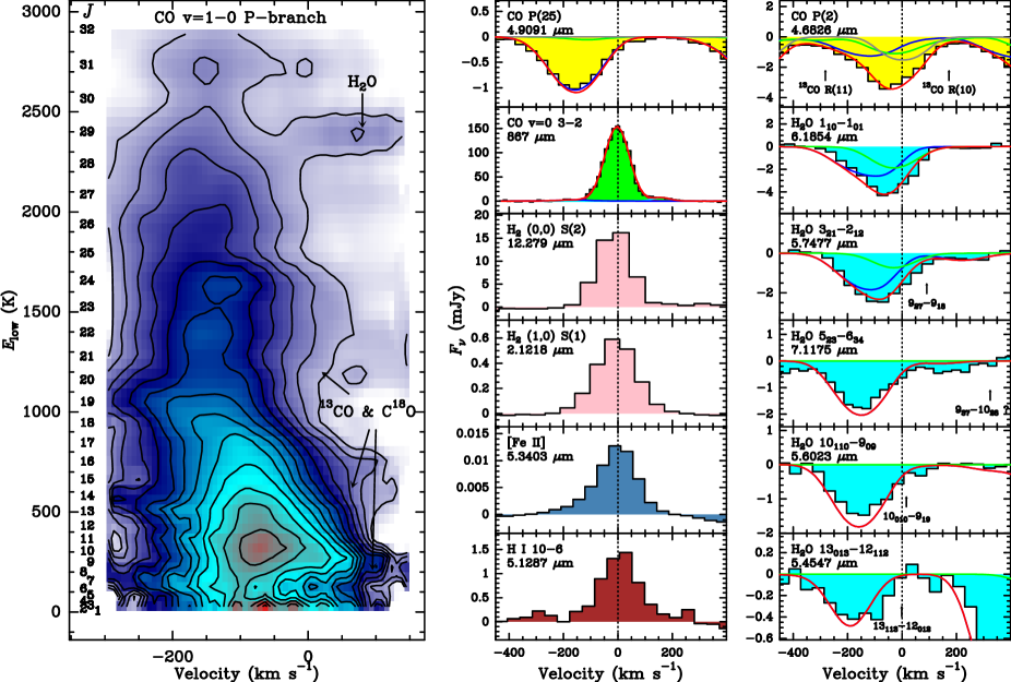
Figure 3: Left: $E_{\mathrm{low}}$-velocity diagram for the CO P-branch lines in VV 114 SW-s2. Contamination by adjacent ¹³CO (together with C¹⁸O) and H₂O lines is indicated on the red side of the profiles. The numbers on the left side indicate the rotational quantum number $J$ of the lower level. Middle and right: Comparison of the profiles of several CO and H₂O ro-vibrational lines (in yellow and light-blue, respectively) and the profiles of CO $v=0\,J=3-2$ line observed with ALMA (green, with a Gaussian fit to the line profile in red), and of several lines of H₂ (pink) and hydrogen recombination line (brown). Prediction by our composite models for the ro-vibrational lines is overlaid.

3 Analysis

3.1 The obscured continuum and the foreground extinction

We constrain the properties of the continuum source behind the observed absorbing gas, specifically its apparent temperature (i.e. once the continuum has been extinguished by intervening dust, $T_{\mathrm{app}}$), the mid-IR extinction (which we characterize by the optical depth at $6\,\mu$m, $\tau_{\mathrm{6\mu m}}^{\mathrm{ext}}$), and the intrinsic shape described by an equivalent blackbody temperature, $T_{\mathrm{bck}}$.

Assuming no reemission in the CO band, the P(J)-to-R(J) peak absorption ratio is $f_{J}\equiv\mathrm{P(J)/R(J)}=F_{\mathrm{c}}^{\mathrm{P(J)}}/F_{\mathrm{c}}^{\mathrm{R(J)}}$ when the lines are optically thick, and $f_{J}=(F_{\mathrm{c}}^{\mathrm{P(J)}}B_{\mathrm{lu}}^{\mathrm{P(J)}})/(F_{\mathrm{c}}^{\mathrm{R(J)}}B_{\mathrm{lu}}^{\mathrm{R(J)}})$ in the optically thin limit. Here $F_{\mathrm{c}}^{\mathrm{P(J)}}$ ($F_{\mathrm{c}}^{\mathrm{R(J)}}$) is the flux density of the continuum behind the absorbing gas at the wavelength of the P(J) (R(J)) transition after foreground extinction, and $B_{\mathrm{lu}}^{\mathrm{P(J)}}$ ($B_{\mathrm{lu}}^{\mathrm{R(J)}}$) is the Einstein coefficient for absorption of radiation in the P(J) (R(J)) transition. Using blackbody emission at temperature $T_{\mathrm{app}}$ to describe the $F_{\mathrm{c}}$ ratios, we compare the theoretical curves for $T_{\mathrm{app}}=330$, 400, and 450 K, with the observed $f_{J}$ values in Fig. 4b. The latter are modulated by ¹³CO contamination in the P-branch and severe blending in the R-branch, but the observed positive slope favors the range $T_{\mathrm{app}}=330-450$ K for $J\geq 10$. This is consistent with the shape of the observed continuum between $4.4-5.0$ $\mu$m ($390$ K, Appendix B), indicating that the continuum behind the CO absorbing gas is, once attenuated by foreground dust, similar in shape to the observed continuum in Fig. 1g.

A similar approach cannot be reliably applied to the H₂O band due to severe line blending, but an estimate of $T_{\mathrm{app}}$ can be obtained by comparing the observed peak absorption of specific spectral features across the band with the corresponding values obtained from models that accurately account for line blending (Section 3.2). Up to 116 spectral features are considered in Fig. 4c-d (and marked on the spectrum in Fig. 9), covering most of the band extent. LTE model results (Sect. 3.2) with $T_{\mathrm{app}}=400$ and 600 K are compared with data in Fig. 4c-d, indicating that the $T_{\mathrm{app}}\sim 400$ K found for CO fails at the long wavelength end of the H₂O band, because the H₂O P-branch lines at $>6.9$ $\mu$m are systematically overestimated. These features are better reproduced with $T_{\mathrm{app}}=600$ K, although the H₂O R-branch features at $<5.4$ $\mu$m are then overestimated. LTE models for the H₂O band favour $T_{\mathrm{app}}\gtrsim 500$ K along the P-branch ($\lambda>6.8$ $\mu$m).

The continuum behind the H₂O band thus flattens relative to that behind the CO band. To explain this effect, invoking a distribution of dust temperatures ($T_{\mathrm{dust}}$) is disfavoured because usually, the longer the wavelength, the lower the $T_{\mathrm{dust}}$ being traced, but the effect found here is the opposite. The increasing $T_{\mathrm{app}}$ with increasing $\lambda$ is better ascribed to differential extinction. The mid-IR extinction laws derived by Indebetouw et al. (2005) and Chiar & Tielens (2006), which we use hereafter (see also Xue et al., 2016), show a drop of $A_{\lambda}$ from near- to mid-IR wavelengths, but the drop is only $\approx 8$% along the CO band between $\sim 4.4$ and 5 $\mu$m. High values of $\tau_{\mathrm{6\mu m}}^{\mathrm{ext}}=2.5-3$ are then required to shape an intrinsic continuum with $T_{\mathrm{bck}}\gtrsim 550$ K to $T_{\mathrm{app}}\sim 400$ K (Appendix D).

The mid-IR spectral energy distribution (SED) in Fig. 1g is consistent with the proposed extinction of the continuum associated with the bands. We fitted the SED using a modified version of the routine by Donnan et al. (2023) (see also García-Bernete et al., 2022), with a minimum number of three blackbody components, the PAHs, and ice absorption. The fit in Fig. 1g fixes $T_{\mathrm{bck}}=550$ K and $\tau_{\mathrm{6\mu m}}^{\mathrm{ext}}=2.5$ for the component that dominates the hot dust emission between 3.5 and 8 $\mu$m (in light-blue). Between 4.4 and 5.0 $\mu$m, $\tau^{\mathrm{ext}}$ varies between 2.7 and 2.9, shaping the continuum to an apparent $T_{\mathrm{app}}\approx 420$ K across the CO band in rough agreement with the value derived from the CO P-R asymmetry (see also Appendix D). We adopt below these fiducial values for the models of the CO and H₂O bands, noting however that the source of mid-IR continuum must not necessarily be a blackbody, but could be diffuse emission with an equivalent temperature as quoted above. We will return to this point in Section 3.2.1.

Table 1: Properties of the components used to model the CO and H₂O fundamental bands in VV 114 SW-s2

	$N_{\mathrm{CO}}$	$N_{\mathrm{H_{2}O}}$	$A_{\mathrm{CO}}$	$A_{\mathrm{H_{2}O}}$	$V_{\mathrm{tur}}$	$V_{\mathrm{gas}}$	$d/R_{\mathrm{IR}}$	$\Delta R/R_{\mathrm{IR}}$	$n_{\mathrm{H_{2}}}$	$T_{\mathrm{gas}}$
	($10^{19}$ cm-2)	($10^{19}$ cm-2)	(pc2)	(pc2)	(km s-1)	(km s-1)			($10^{5}$ cm-3)	(K)
$H_{C}$	$1.8-3.5$	$1.5-3.0$	$0.14-0.25$	$0.11-0.20$	60	$300-50$	0	$\lesssim 0.5$
$W_{C}$	$0.5-1.2$	$0.1-0.4$	$0.11-0.20$	$0.07-0.12$	60	$30$	$\gtrsim 2$	$-$	$1-5$	$300$
$C_{C}$	$\sim 1$	$-$	$>0.14$	$-$	60	$0$	$-$	$-$	$\sim 1$	$10$

3.2 The best fit to the CO and H₂O bands

Our model for the bands includes the three components outlined in Section 2.1: the $H_{C}$ generating absorption in the highest energy lines, the $W_{C}$ dominating the absorption at lower energy, and the $C_{C}$, only for CO, which produces additional absorption in the lowest $J$ lines. We use the code described in González-Alfonso et al. (1998), which assumes spherical symmetry. It has been updated to generate modeled spectra convolved with the JWST/NIRSpec and MIRI/MRS spectral resolution. The calculations include a careful treatment of overlaps among lines of the same or different species.

We start modeling the $H_{C}$ by assuming thermalization of all levels in the ground vibrational state at $T_{\mathrm{rot}}$ with no significant population in the upper vibrational state. The only free parameters in LTE models are $T_{\mathrm{rot}}$, $N_{\mathrm{CO}}$ (including ¹³CO with $\mathrm{[^{12}CO]/[^{13}CO]=30-60}$), $N_{\mathrm{H_{2}O}}$, and the gas velocity field. We considered two different approaches for the latter: $V_{\mathrm{field}}^{\mathrm{A}}$ denotes a combination of turbulent velocity ($V_{\mathrm{tur}}=60$ km s^-1) and a velocity gradient across the shell, and $V_{\mathrm{field}}^{\mathrm{B}}$ uses a constant outflowing velocity of 190 km s^-1 with a small $V_{\mathrm{tur}}=20$ km s^-1. In the latter case, to match the observed linewidths, the profiles were convolved with a Gaussian distribution of velocities, simulating an ensemble of clumps with a velocity distribution along the line of sight.

Radiative transfer calculations were also performed to infer which physical conditions are required to explain the observed excitation and absorption in the $H_{C}$. Models with collisional excitation alone, simulating shocked gas detached from the mid-IR source, and models including radiative pumping simulating gas in close proximity to the mid-IR source behind it, were generated. In the calculation of line fluxes, the shell is truncated on the flanks around the central source as required to avoid line reemission (see Fig. 8 in González-Alfonso et al., 2014b). Statistical equilibrium calculations were performed using the rates by Yang et al. (2010) for collisional excitation of CO with H₂, and those by Daniel et al. (2011) for H₂O with H₂, both extrapolated to higher energy levels with the use of an artificial neural network (Neufeld, 2010).

The $W_{C}$ is modeled as a shell of gas surrounding the mid-IR source expanding at a velocity of 30 km s^-1. A set of models was generated by changing the distance from the surface of the central source to the shell ($d$), the H₂ density and gas temperature ($n_{\mathrm{H_{2}}}$ and $T_{\mathrm{gas}}$), and the CO and H₂O column densities ($N_{\mathrm{CO}}$, $N_{\mathrm{H_{2}O}}$). To match the line profiles, $V_{\mathrm{tur}}=90$ km s^-1 was used (giving $\mathrm{FWHM}=150$  km s^-1 for optically thin lines).

All combinations among the $W_{C}$ and $H_{C}$ model components were cross-matched with the data by computing $\chi^{2}$ for the peak absorption features (Fig. 4). Minimization of $\chi^{2}$ gives the area that CO and H₂O have in the plane of sky, $A_{\mathrm{CO}}$ and $A_{\mathrm{H_{2}O}}$, in both components, and thus the minimum area of the mid-IR continuum source behind it. The derived parameters are listed in Table 1. Figures 2, 3, and 11 overlay the resulting best-fit model profiles on the observed spectra, and Fig. 4 compares the observed peak absorption with the best-fit model predictions. The models also give the strength of the continuum behind each component, shown with dashed lines in Fig. 1g, as required to match the absolute absorption fluxes.

3.2.1 The Hot component

Extremely high column densities for both CO and H₂O are required to explain the observed absorption strengths in the outflowing $H_{C}$. The minimum values of both $N_{\mathrm{CO}}$ and $N_{\mathrm{H_{2}O}}$ are found in LTE models with $V_{\mathrm{field}}^{\mathrm{B}}$: $\approx 1.5\times 10^{19}$ cm^-2 at $T_{\mathrm{rot}}\approx 450-500$ K. In CO, these are required to account for $(i)$ the small contrast between the absorption strengths of intermediate $J=15-22$ and high $J>25$ lines, indicating that the former lines are optically thick; $(ii)$ the absorption in the ¹³CO P(18)-P(19) lines, further indicating optically thick absorption in the same lines of ¹²CO, and $(iii)$ the blueshifted wings observed in the low-$J$ lines.

In models with pure collisional excitation, additionally extremely high densities of $>10^{9}$ cm^-3 are needed to explain the H₂O excitation, due to the high $A-$Einstein coefficients and critical densities of the H₂O rotational transitions. The combination of such high $n_{\mathrm{H_{2}}}$, $T_{\mathrm{gas}}$, and $N_{\mathrm{CO,H_{2}O}}$ raises strong interpretation problems in the framework of shock models where molecules are collisionally excited. We have used the Paris-Durham shock code (e.g. Godard et al., 2019) to generate both $C-$type and $J-$type shock models for a variety of pre-shock densities, magnetic fields, and shock velocities, but failed to reproduce the required column densities of warm molecular gas. Multiple ($>20$) shocked spots along the line of sight would be required to attain the required columns at high $T_{\mathrm{gas}}$, but the necessary pre-shock densities of $\gtrsim 10^{8}$ cm^-3 would in any case indicate that the shock is produced very close to the source of IR radiation.

On the other hand, the models that include excitation by the mid-IR source at $\sim 550$ K naturally yield $T_{\mathrm{rot}}\approx 450-500$ K as required by LTE models, provided that the molecular shell is in close proximity to the mid-IR source, and that the latter is a blackbody in the mid-IR. We conclude that the observed bands are closely associated with the mid-IR continuum behind it and that the excitation of the CO and H₂O rotational levels of the ground vibrational state is influenced by radiative excitation. Indeed we find that the effect of mid-IR pumping is so strong that results for the bands are basically insensitive to $n_{\mathrm{H_{2}}}$ and $T_{\mathrm{gas}}$, and only depend on $T_{\mathrm{bck}}$, $N_{\mathrm{CO,H_{2}O}}$, the width of the absorbing shell, and the velocity field. In our best-fit model shown in Figs. 2, 3, 4, and 11, $N_{\mathrm{CO}}=3.5\times 10^{19}$ cm^-2, $N_{\mathrm{H_{2}O}}=3.0\times 10^{19}$ cm^-2, $\Delta R/R_{\mathrm{IR}}=0.3$, and $V_{\mathrm{field}}^{\mathrm{A}}$ is used. As indicated in Table 1, the effective size of the absorbing shell is sub-pc.

The strength of the continuum behind the different components as well as $A_{\mathrm{CO,H_{2}O}}$, depend on the gas velocity field and shell width, and cannot be constrained to better than 50%. Nevertheless, our best-fit models indicate that the sum of the continuum behind $H_{C}$ and $W_{C}$ as derived from CO is similar to the continuum due to hot dust predicted by our fit to the mid-IR emission (Fig. 1g).

3.2.2 The Warm component

The $W_{C}$ most likely involves a mix of several components peaking close to the reference velocity, such as material at the surface of the IR source that is not covered by the $H_{C}$, gas in front of the IR source more distant than the $H_{C}$, and gas on the flanks that is illuminated and reemits preferently in the P($J<10$) lines of CO. An additional difficulty comes from the fact that the $H_{C}$ and $W_{C}$ partially overlap in velocity, and their relative contribution to the moderate excitation lines is uncertain to some extent. Here we explore whether gas in front of the IR source can account for the remaining absorption unmatched by the $H_{C}$. Because of the lower $W_{C}$ excitation relative to the $H_{C}$, the warm gas is in this scenario at a distance of $\gtrsim 2R_{\mathrm{IR}}$ from the surface of the IR source. The excitation is in this case sensitive to $n_{\mathrm{H_{2}}}$ and $T_{\mathrm{gas}}$, but is still also affected by the radiation field. Our results enable the interpretation of the $W_{C}$ as an extension of the $H_{C}$ further from the IR source, and could represent the shock produced by the inner outflow ($H_{C}$) as it sweeps out the surrounding ambient gas ($C_{C}$), or the remnant of a previous outflowing pulse. The latter is favored due to the discontinuity in excitation between the $H_{C}$ and the $W_{C}$, as readily seen in the overall CO band shape.

3.2.3 The Cold component

As noted in Section 2.1, the CO band shows strong absorption in the $J\leq 3$ lines, indicating the presence a cold component ($C_{C}$) in front of the continuum source. $C_{C}$ is modeled with a screen approach as a cold slab with $N_{\mathrm{CO}}=1\times 10^{19}$ cm^-2, $n_{\mathrm{H_{2}}}=1\times 10^{5}$ cm^-3, and $T_{\mathrm{gas}}=10$ K. These parameters are relatively uncertain because $C_{C}$ is most likely absorbing a continuum that has already been partially absorbed by the $W_{C}$ at similar velocities, and the model does not simulate this effect. $C_{C}$ also shows up in the ¹³CO P(1) and P(2) lines, blueshifted relative to ¹²CO P(13) and P(14) (Fig. 11).

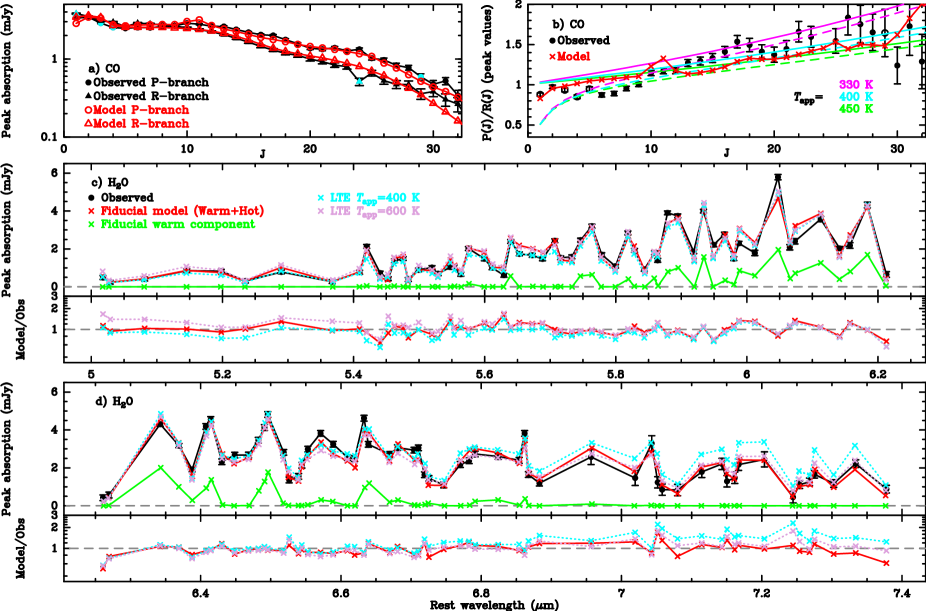
Figure 4: a) Peak absorption values of the CO P(J) (circles) and R(J) (triangles) lines. Black filled symbols indicate data, and red symbols show the model prediction. Light-blue markers indicate contaminated lines. b) CO P-R asymmetry for the peak absorption values. Black circles indicate data, with opened symbols indicating doubtful ratios due to contaminating lines other than ¹³CO. Red crosses show model results. The magenta, light-blue, and green curves display the expected trends for several $T_{\mathrm{app}}$ values in the optically thick (solid) and optically thin (dashed) limits. c-d) Comparison between the H₂O peak absorption of 116 spectral features (black circles) and our fiducial model. The contribution by the warm component is shown in green, and the total predicted absorption (warm+hot components) is shown in red. LTE model results with $T_{\mathrm{app}}=400$ and 600 K, $T_{\mathrm{rot}}=450$ K, and $N_{\mathrm{H_{2}O}}=3\times 10^{19}$ cm^-2 (the same $N_{\mathrm{H_{2}O}}$ as in the fiducial model) are also compared with data. The model-to-observed peak absorption ratios are also displayed. Errorbars in this figure do not include uncertainties from continuum subtraction.

4 Discussion and conclusions

4.1 Energetics

The extremely high column densities found for the $H_{C}$ indicate that the observed absorption is most likely dust-limited. At 6 $\mu$m the mass absorption coefficient is $\approx 15$ times higher than at 100 $\mu$m. Using the $N_{\mathrm{H}}-\tau_{\mathrm{100\mu m}}$ relationship in González-Alfonso et al. (2014a), we expect $\tau_{\mathrm{6\mu m}}=1$ for $N_{\mathrm{H}}\sim 10^{23}$ cm^-2, and our derived CO and H₂O column densities in the $H_{C}$ of $\mathrm{a\,few}\,\times 10^{19}$ cm^-2 roughly give the quoted $N_{\mathrm{H}}$ for abundances of $\mathrm{a\,few}\,\times 10^{-4}$. We could thus be still missing outflowing material behind the curtain of dust.

Adopting $N_{\mathrm{H}}\sim 10^{23}$ cm^-2, the gas mass of the outflowing $H_{C}$ is $M_{H_{C}}=\mu m_{\mathrm{H}}A_{\mathrm{CO}}N_{\mathrm{H}}\approx 170\,M_{\odot}$, where $\mu=1.36$ accounts for elements other than hydrogen and we have used the minimum value of $A_{\mathrm{CO}}$ in Table 1. In spite of the high column densities, the small size yields a low mass that makes the $H_{C}$ undetectable in the CO rotational lines at millimeter wavelengths (Sect. 2.1).

The mass outflow, momentum, and energy rates can be estimated as time-averaged or instantaneous values, depending on whether the outflowing shell radius $R$ or the shell width $\Delta R$ are used in the equations (Rupke et al., 2005; González-Alfonso et al., 2017; Veilleux et al., 2017). Adopting here the (higher) instantaneous values with $\Delta R\sim 0.1$ pc, we obtain $\dot{M}_{H_{C}}\sim 0.3\,M_{\odot}\,\mathrm{yr^{-1}}$, $\dot{P}_{H_{C}}\sim 3.6\times 10^{32}$ dyn, and $\dot{E}_{H_{C}}\sim 3.2\times 10^{39}$ erg s^-1. These estimates are likely lower limits, but indicate rather moderate momentum and energy rates as compared with the radiation pressure and IR luminosity (see below), $\dot{P}_{H_{C}}/(L_{\mathrm{IR}}/c)\sim 0.4$ and $\dot{E}_{H_{C}}/L_{\mathrm{IR}}\sim 10^{-4}$. Therefore, radiation pressure can drive the observed outflow.

4.2 The origin of the bands

A crucial point of our analysis is that the rotational levels of the ground vibrational state of CO and H₂O are radiatively excited by the mid-IR continuum, and thus this continuum is optically thick -i.e. a true mid-IR blackbody with temperature $T_{\mathrm{bck}}\approx 550$ K. On the other hand, the extreme CO and H₂O excitation and specific kinematics of the $H_{C}$ indicate a common environment, and thus the area covered by the outflow in the plane of sky is most likely of the same order as the effective areas listed in Table 1. This implies that the obscured hot blackbody emission forms a coherent, connected structure.

The size of this coherent bright object can be estimated from the sum of the areas $A_{\mathrm{CO}}(H_{C})+A_{\mathrm{CO}}(W_{C})$, giving $R_{\mathrm{IR}}=0.31$ pc, which assumes that both areas do not overlap. We estimate the luminosity of this sub-pc structure as $L_{\mathrm{IR}}=(2-4)\times(A_{\mathrm{CO}}(H_{C})+A_{\mathrm{CO}}(W_{C}))\sigma T_{\mathrm{bck}}^{4}$, where the numerical factors correspond to a disk seen face-on and a sphere, respectively, giving $\sim(0.8-1.7)\times 10^{10}\,L_{\odot}$. The luminosity surface density is given by $\Sigma_{\mathrm{IR}}=\sigma T_{\mathrm{bck}}^{4}\approx 1.3\times 10^{10}$ $L_{\odot}$ pc^-2. The areas and $L_{\mathrm{IR}}$ scale with foreground extinction as $\propto\exp\{\tau_{\mathrm{6\mu m}}^{\mathrm{ext}}-2.5\}$. Because of possible departures from blackbody emission, lower $T_{\mathrm{dust}}$ behind the area covered by the $W_{C}$, and beaming effects (see below), we write

$$L_{\mathrm{IR}}\approx(1\pm 0.5)\times 10^{10}\,\exp\{\tau_{\mathrm{6\mu m}}^{\mathrm{ext}}-2.5\}\,L_{\odot}.$$ (1)

We remark that the estimated value $\Sigma_{\mathrm{IR}}\sim 10^{10}$ $L_{\odot}$ pc^-2, which is compared below with the values in other sources, is not based on direct measurements of the source size. The SW-s2 clump, as seen with the ALMA angular resolution of $0.14^{\prime\prime}\approx 60$ pc, cannot be used to constrain the properties of the extremely compact source of mid-IR emission; indeed, the measured 345 GHz continuum flux density (Fig 1b,f) is $\approx 1$ mJy beam^-1, and a blackbody of 550 K and radius $0.31$ pc gives $0.08$ mJy. The CO and H₂O molecular bands are used as a surrogate for spatial resolution, enabling us to identify high concentrations of hot dust and to estimate $\Sigma_{\mathrm{IR}}$ on the assumption of a connected structure for the associated mid-IR emission.

We compare the physical properties derived for VV 114 SW-s2 with those found for the galactic massive ($\sim 45\,M_{\odot}$), luminous ($1\times 10^{5}\,L_{\odot}$) isolated protostar AFGL 2136 IRS 1, which has been also observed in the CO $v=1-0$ band (Mitchell et al., 1990) and in the H₂O $\nu_{2}$, $\nu_{1}$ and $\nu_{3}$ fundamental bands from the ground and with the EXES instrument on SOFIA, with all IR lines in absorption (Indriolo et al., 2013, 2020; Barr et al., 2022). The bands and the associated near- to mid-IR continuum probe a Keplerian disk around the protostar. A large-scale bipolar outflow is observed in CO at millimeter wavelengths with velocities $\lesssim 20$ km s^-1 (Kastner et al., 1994), but not in the ro-vibrational lines of CO or H₂O. The inner disk has been resolved in the H₂O $\nu_{2}=1-1\,5_{50}-6_{43}$ line with ALMA, giving a radius of 120 au (Maud et al., 2019). Using $R_{\mathrm{IR}}=0.31$ pc and $L_{\mathrm{IR}}=1.7\times 10^{10}\,L_{\odot}$ for VV 114 SW-s2, we find that the ratio of SW-s2 to AFGL 2136 luminosities, $\sim 1.7\times 10^{5}\exp\{\tau_{\mathrm{6\mu m}}^{\mathrm{ext}}-2.5\}$, is similar to the ratio of squared sizes, $2.8\times 10^{5}\exp\{\tau_{\mathrm{6\mu m}}^{\mathrm{ext}}-2.5\}$, indicating similar continuum brightness. Indeed, the rotational temperature derived from the H₂O absorption in AFGL 2136 IRS 1, $\sim 520$ K (Indriolo et al., 2020), is remarkably close to our derived $T_{\mathrm{bck}}\approx 550$ K. Therefore, VV 114 SW-s2 behaves in continuum brightness as the inner hot disk around a high-mass protostar (another aspect of the analogies found between protostars and buried galaxy nuclei; Dudley & Wynn-Williams, 1997; Gorski et al., 2023), but with a projected area $\gtrsim 10^{5}\exp\{\tau_{\mathrm{6\mu m}}^{\mathrm{ext}}-2.5\}$ times larger, and with the CO and H₂O fundamental bands, rather than tracing a stationary disk/torus, outflowing at $V_{\mathrm{out}}\approx 180$ km s^-1. While the flow timescale is only $R_{\mathrm{IR}}/V_{\mathrm{out}}\sim 1.7\times 10^{3}$ yr, an upper limit is constrained by $M_{\mathrm{gas}}(H_{C})/\dot{M}_{H_{C}}\lesssim 10^{6}$ yr. Whatever is the source of power heating the dust and driving the outflow in VV 114 SW-s2, it is caught in a very early phase of evolution where feedback has not yet been able to clear the natal cocoon, at least on the side facing the observer.

Another source of comparison, with a spatial scale more akin to VV 114 SW-s2, is the proto-super star cluster 13 (p-SSC13) in NGC 253. Rico-Villas et al. (2022) observed this source with high angular resolution ($0.02^{\prime\prime}\approx 0.4$ pc) in the millimeter continuum and in a suite of HC₃N rotational lines from the ground and excited vibrational states, up to $\nu_{6}=2$ ($>1500$ K). They found that p-SSC13, with radius $\approx 1.5$ pc, is extremely buried ($\sim 10^{25}$ cm^-2), and trapping of continuum photons raises the inner $T_{\mathrm{dust}}$ such that the pumping of the HC₃N excited vibrational states is very effective (i.e. the greenhouse effect, González-Alfonso & Sakamoto, 2019). As a result, the inferred $L_{\mathrm{IR}}$ and $\Sigma_{\mathrm{IR}}$ remain moderate ($\approx 10^{8}\,L_{\odot}$ and $\approx 10^{7}\,L_{\odot}$ pc^-2, respectively). We note that, while the millimeter high-excitation HC₃N lines are not extinguished and thus probe the inner thermal structure of p-SSC13, the CO and H₂O bands seen in absorption and blueshifted in VV 114 SW-s2 are surface tracers, revealing the actual $\Sigma_{\mathrm{IR}}\sim 1\times 10^{10}\,L_{\odot}$ pc^-2 associated with the outflowing gas.

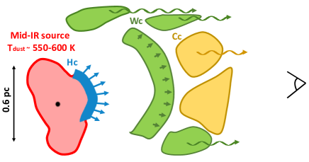
Figure 5: Sketch of VV 114 SW-s2. The 3 components used in the modeling, $H_{C}$, $W_{C}$, and $C_{C}$, are represented in blue, green, and orange, respectively. The outflow takes places in the polar direction.

Rico-Villas et al. (2022) found that the $\Sigma_{\mathrm{IR}}\sim 10^{7}\,L_{\odot}$ pc^-2 value derived for p-SSC13 ocuppies an intermediate position between galactic star-forming regions and bright (U)LIRGs (where values up to $\sim 10^{8.3}\,L_{\odot}$ pc^-2 have been derived for the nuclear $<100$ pc regions, Pereira-Santaella et al., 2021). Since massive star formation in p-SSC13 is taking place very efficiently, its $\Sigma_{\mathrm{IR}}$ was taken as a proxy for the most extreme starburst at $\gtrsim 0.1$ pc spatial scales. On this basis, the $\Sigma_{\mathrm{IR}}\sim 10^{10}\,L_{\odot}$ pc^-2 of VV 114 SW-s2 can be most easily understood as a black hole (BH) in a very early stage of accretion and feedback.

Our identification of VV 114 SW-s2 as an AGN finds support in the observation of the CO $v=1-0$ band in IRAS 08572$+$3915 NW by Onishi et al. (2021). This source is a well known AGN-dominated ULIRG with $L_{\mathrm{AGN}}\sim 10^{12-13}\,L_{\odot}$ (Veilleux et al., 2009; Efstathiou et al., 2014). The observations covered CO band lines from R(26) to P(19), showing one very excited and broad velocity component blueshifted by $-160$ km s^-1 relative to systemic, presumably arising from the innermost region of the torus surrounding the AGN (component (a) in Onishi et al., 2021). The blueshift of this component is very similar to that found for the $H_{C}$ of SW-s2. Concerning the excitation, the peak absorption observed in IRAS 08572$+$3915 NW decreases from $\approx 30$% of the observed continuum for the R(20) line to $\approx 10$% for the R(25) line, while in SW-s2 the absorption decreases more slowly with increasing $J$, from $\approx 20$% (R(20)) to $\approx 12$% (R(25)) (Fig. 11). Thus CO appears to be similarly or even more excited in SW-s2 than in IRAS 08572$+$3915 NW.

4.3 Lifetime constraints and the mass of the BH

Assuming Eddington luminosity, the BH mass is $M_{\mathrm{BH}}\sim 3\times 10^{5}\exp\{\tau_{\mathrm{6\mu m}}^{\mathrm{ext}}-2.5\}\,M_{\odot}$, but we can refine this estimate because the derived luminosity is not necessarily Eddington and, as shown below, constraining the BH evolving time $t$ is equivalent to constraining $M_{\mathrm{BH}}$. To apply a limit to the BH growing time in SW-s2 we assume that the BH has evolved locally from the seed (with adopted initial mass $M_{\mathrm{BH,0}}=100\,M_{\odot}$) so that the BH evolving time cannot be longer than the lifetime of its s2 host. The high concentration of CO cold gas at the s2 clump (Fig. 1a,d) and the high column densities of hot molecular gas strongly suggest that this is the case, supporting also the assumption that the main channel of BH growth in SW-s2 is gas accretion.

A first approach for setting the lifetime of the s2 clump is from the works by Linden et al. (2021, 2023), who studied in a large number of clumps of VV 114, including the overlap region, the colors from optical/UV Hubble to near-IR JWST data. By comparing the observed colors with predictions from evolutionary models of stellar population, they found that the most embedded star clusters, undetected in the optical/UV, have lifetimes $t\lesssim 5$ Myr. While the SW-s2 clump undoubtedly belongs to the category of strongly embedded sources, it may not represent the majority of star clusters in the Linden et al. (2023) sample, because of its location at the head of the filament (Fig. 1a). The merger-induced shocked gas at the overlap region (Saito et al., 2015) may lose angular momentum and flow along the filament, replenishing the nuclear region of VV 114 E and specifically the SW-s2 clump. Unfortunately, the method used by Linden et al. (2023) to estimate the age of the clusters, which mostly relies on the blue to red supergiant transition traced by the $\mathrm{F150W-F200W}$ color, cannot be applied to SW-s2 because its F200W ($2\,\mu$m) emission is at the background level (Fig. 1c).

On the other hand, it is clear from our analysis of the spectra and timescales that the observed region is currently evolving very quickly, and that the $H_{C}$ may indeed represent a peak of activity. On longer time scales the head of the VV 114 E appears to be evolving quickly as well, with separated spots that have not yet coalesced. In addition, the s2 clump appears off-center with brighter regions in NE and SW-s1, suggesting that s2 is relatively young. The depletion timescale for the dense gas in s2 is $\sim 6$ Myr (the S5 “box” in Saito et al., 2015). Simulations of super star cluster formation and evolution (Skinner & Ostriker, 2015), which is the most likely environment for BH seed formation and growth (e.g., Portegies Zwart & McMillan, 2002; Gürkan et al., 2004; Goswami et al., 2012), indicate that the bulk of the initial reservoir of gas is locked into stars or ejected after $\sim 5t_{\mathrm{ff}}$, ($t_{\mathrm{ff}}$ is the initial free-fall time), and thus the gas surface density significantly decreases afterwards. Using the extraction radius of the CO (3-2) profile in SW-s2 ($r=70$ pc) and the gas mass inferred from the line flux ($\sim 3\times 10^{7}\,M_{\odot}$), $t_{\mathrm{ff}}=1.8\times(1+M_{*}/M_{\mathrm{gas}})^{-1/2}$ Myr and we thus expect $t\lesssim 9$ Myr in view of the still embedded stage of the clump. All in all, we propose a fiducial conservative timescale for the BH growth in SW-s2 of $t\sim 10$ Myr, with an uncertainty of a factor $\sim 2$ to accommodate more extreme cases (see Fig 4 in Linden et al., 2023).

The simple BH growth model in Appendix F shows that the quoted time constraint translates into an $e-$folding time of $t_{0}\sim 2^{+2}_{-1}$ Myr, and using the relationship between AGN luminosity and accretion rate by Watarai et al. (2000) (also used by Toyouchi et al., 2021), we arrive at

$$M_{\mathrm{BH}}\sim\frac{3.7\times 10^{4}\,M_{\odot}}{1-0.244\ln t_{0}}\,\exp\{\tau_{\mathrm{6\mu m}}^{\mathrm{ext}}-2.5\},$$ (2)

where $t_{0}$ is in Myr. Because of the weak dependence on $t_{0}$, this result favors an IMBH in SW-s2:

$$M_{\mathrm{BH}}=(4.5\pm 2.4)\times 10^{4}\exp\{\tau_{\mathrm{6\mu m}}^{\mathrm{ext}}-2.5\}\,M_{\odot},$$ (3)

where the quoted error includes uncertainties in $t_{0}$ and $L_{\mathrm{IR}}$ added in quadrature. Both the current accretion rate ($\dot{M}_{\mathrm{BH}}/\dot{M}_{\mathrm{Edd}}\sim 25$) and luminosity ($L/L_{\mathrm{Edd}}\sim 7$) are super-Eddington, with $\dot{M}_{\mathrm{BH}}\sim 2.4\times 10^{-2}\exp\{\tau_{\mathrm{6\mu m}}^{\mathrm{ext}}-2.5\}$ $M_{\odot}$ yr^-1. If the $H_{C}$ represents a peak of activity with the current $L/L_{\mathrm{Edd}}$ above the time-averaged value, $M_{\mathrm{BH}}$ will be lower than in eq. (3).

Detailed 3D simulations of super-Eddington accretion onto IMBHs, limited to low metallicities ($Z\leq 0.1Z_{\odot}$) and $M_{\mathrm{BH}}=10^{4}\,M_{\odot}$, have been performed by Toyouchi et al. (2021) (see also Inayoshi et al., 2016, for extreme BH growth in metal poor environments). These models yield super-Eddington accretion if the dusty disk becomes optically thick to ionizing radiation, as is most likely the case for SW-s2. Toyouchi et al. (2021) calculated, over an elapsed time of $\lesssim 10$ Myr, both the time-averages of mass accretion rate onto the BH ($\langle\dot{M}_{\mathrm{BH}}\rangle$) and mass outflow rate ($\langle\dot{M}_{\mathrm{out}}\rangle$), as a function of the Eddington-normalized mass injection rate from the outer source boundary ($\dot{M}_{\mathrm{in}}/\dot{M}_{\mathrm{Edd}}$). Their $Z=0.1\,Z_{\odot}$ model that better resembles our results for SW-s2 has $\dot{M}_{\mathrm{in}}/\dot{M}_{\mathrm{Edd}}=10$, yielding $\langle\dot{M}_{\mathrm{out}}\rangle/\langle\dot{M}_{\mathrm{BH}}\rangle\approx 6$. The outflow, driven by radiation pressure on dust grains (as for the $H_{C}$, Section 4.1), takes places in the polar direction and is time-variable (as also favored for SW-s2, Section 3.2.2). Our result for the mass outflow rate of the $H_{C}$ ($\dot{M}_{H_{C}}\gtrsim 0.3\,M_{\odot}\,\mathrm{yr^{-1}}$) yields a comparable $\dot{M}_{H_{C}}/\dot{M}_{\mathrm{BH}}\gtrsim 12$, although models with higher metallicities (Saito et al., 2015) are required to refine this comparison. According to Shi et al. (2023), the global SW-s2 conditions required for a significant chance of runaway BH growth via gas accretion are met ($\Sigma_{\mathrm{gas}}\gtrsim 10^{3}$ $M_{\odot}$ pc^-2, $M_{\mathrm{gas}}>10^{6}$ $M_{\odot}$).

VV 114 SW-s2 possibly exemplifies the IMBH to SMBH transition in the evolved Universe, diagnosed in the mid-IR as sub-pc fully-enshrouded cocoons of hot dust where outflows have not yet been able to evacuate the polar regions to form an open torus. The cartoon in Fig. 5 shows a possible schematic geometry of the relative locations of the components observed in the CO and H₂O bands. The JWST observations of VV 114 E suggest that IMBHs/SMBHs can be formed throughout the merging process in distinct nuclear clumps of the same merging galaxy, and could coalesce afterwards.

The unprecedented sensitivity and spectral resolution of JWST enable detection of this type of buried object in extragalactic sources. Ongoing and future observations will reveal how common they are, and how they evolve.

Appendix A Data reduction

JWST imaging and integral field spectroscopy (IFU) of VV 114 were taken as part of the Director’s Discretionary Early Release Science (DD-ERS) Program ID #1328 (PI: L. Armus and A. Evans). MIRI-MRS ($4.9-28.1$ $\mu$m) and NIRSpec-IFU data with the high spectral resolution ($R\sim 2700$) gratings were retrieved, as well as the fully reduced and calibrated NIRCam F200W, and MIRI F560W, F770W, and F1500W images.

The NIRSpec-IFU data of the CO band were obtained with the grating/transmission filter pair G395H/F290LP, using the NRSIR2RAPID readout with 18 groups and a small cycling dither pattern (4 points). The spaxel size is $0.1^{\prime\prime}$. The observations were processed using the JWST Calibration pipeline (version 11.16.20). All details of the reduction procedure are given in García-Bernete et al. (2023) and Pereira-Santaella et al. (2023).

The MIRI-MRS data of the four channels were reduced using the 1.11.0 pipeline version and calibration 1095 of the Calibration Reference Data System. The pixel size is $0.196^{\prime\prime}$ for channels 1 and 2, and increases to $0.245^{\prime\prime}$ for channel 3 with likely contamination by the SWS-s1 core (Fig. 1). For this reason, we show the spectrum in Fig. 1g up to 10 $\mu$m. We primarily followed the standard MRS pipeline procedure (e.g., Labiano et al. 2016, and references therein) and the same steps as described in García-Bernete et al. (2022) and Pereira-Santaella et al. (2022) to reduce the data. Some hot/cold pixels are not identified by the current pipeline, so we added some extra steps as described in Pereira-Santaella et al. (2023) and García-Bernete et al. (2023) for NIRSpec and MRS, respectively.

In order to obtain a continuous near- to mid-IR spectrum of VV 114 SW-s2 (Fig. 1g), the flux densities of all NIRSpec bands were scaled up by a factor of 1.2, due to uncertainties in the relative calibration of both instruments. Specifically, the NIRSpec/G395H spectrum, where the CO band lies, was multiplied by the quoted factor to match the continuum of MIRI/MRS CH1-short in the $4.8-5.2$ $\mu$m overlap region of the two detectors (Fig. 6a).

The lines in common in this overlap region allows us to cross-calibrate the CO and H₂O bands. As shown in Fig. 6a, most of the CO P-branch lines within NIRSpec/G395H appear to be stronger than within MIRI/MRS, after applying the scaling factor. We compare in Fig. 6b the two continuum-subtracted spectra, where the NIRSpec spectrum has not been scaled up, and panel c compares the corresponding CO P(16)-P(28) line absorption fluxes from multi-Gaussian fit to the spectra. From this comparison, the lines within NIRSpec/G395H have not been scaled up by the 1.2 factor.

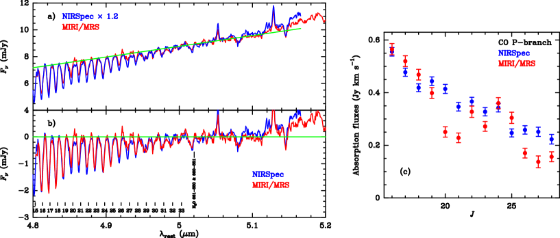
Figure 6: a) NIRSpec G395H and MIRI/MRS CH1-Short spectra of VV114 SW-s2 in the $4.8-5.2$ $\mu$m overlap region. The NIRSpec spectrum has been scaled up by a factor 1.2 to match the MIRI/MRS continuum. The green line is the fiducial baseline used for the CO band. b) Continuum-subtracted spectra, where the NIRSpec spectrum has not been scaled up. c) CO P(16)-P(28) line fluxes from Gaussian fits to the continuum-subtracted spectra of panel b).

Appendix B The baseline of the CO band

The baseline continuum of the CO fundamental band is uncertain mostly across the R-branch, because the lines are broad and blend at their wings forming a pseudo/continuum. A similar effect is seen in the P-branch, because of the contribution by the ¹³CO and C¹⁸O lines to the spectrum. Three alternative baselines are shown in Fig. 7left: the fiducial one in red, which is used in this work, a blackbody at 390 K in blue, and a straight line joining two extreme points of the band, in green. The fiducial one is made up of 2 straight lines with different slopes, joining at $\lambda_{\mathrm{rest}}=4.67$ $\mu$m.

The peak absorption and P/R values obtained with the use of the 3 baselines are compared in Fig. 7right. Comparing values using the fiducial and the straight line baselines, the peak absorption increases by $10-15$% across the P-branch, except for the P(29) and P(30) that show an increase of $18-20$%. Across the R-branch the peak values also increase similarly up to $J=20$, and show a higher increase of $20-30$% for R($J>24$). Therefore, the P/R values remain similar up to $J=20$, and decrease for the highest $J$ slightly as compared with the errorbars shown in Fig. 4b.

Basically, the use of the straight line as the baseline would increase the area covered by CO in all components of Table 1 by $10-15$%. We mostly rely in the fiducial baseline because our models for the CO band predict that, across the P-branch, the continuum level is traced between P(4)-P(5), P(10)-P(11)-P(12)-P(13), and P(16)-P(17)-P(18)-P(19) (Fig. 2).

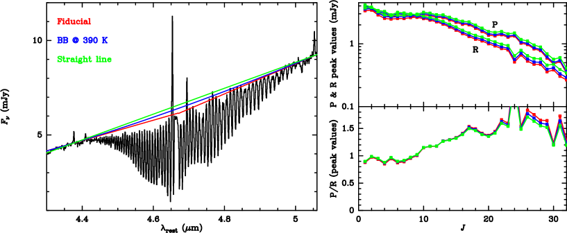
Figure 7: Left: Comparison of considered baselines for the CO band. The red curve is the fiducial baseline we have used in this work. Right-upper: Peak absorption values of the CO P(J) and R(J) lines for the three baselines. Right-lower: The CO P-R asymmetry of the peak absorption values for the 3 baselines.

Appendix C Details on the H₂O band

Figure 8 shows in red all H₂O rotational levels of the ground vibrational state from which at least one ro-vibrational line contributes, according to our best-fit model, to the observed mid-IR spectrum of VV 114 SW-s2. As usual, the diagram is described by means of a series of $J$-ladders. It is well known that collisional excitation of H₂O, when thermal equilibrium breaks down, usually tends to overpopulate the backbone rotational levels (i.e. levels with $J=K_{c}$) at the expense to all others, due to the relatively high optical depths and thus radiative trapping among the rotational lines connecting these levels (e.g. de Jong 1973). Due to the high $A_{\mathrm{ul}}-$Einstein coefficients of the H₂O rotational transitions, this will happen as long as $n(\mathrm{H_{2}})\lesssim 10^{9}$ cm^-3, depending on the column density per unit velocity interval. In VV 114 SW-s2, however, ro-vibrational lines arising from levels distant from backbone are detected (e.g. lines from all $J=6$ levels), as well as ro-vibrational transitions from backbone levels up to $J=13$. This illustrates the extreme excitation of H₂O in the $H_{C}$, and the very high densities and column densities that would be required to explain the observed spectrum via collisional excitation.

The H₂O $\nu_{2}=1-0$ band spectrum is shown in Fig. 9. The observed spectral features are marked with the lower level energy ($E_{\mathrm{low}}$) of the contributing transitions. Particularly crowded is the $6.4-6.8$ $\mu$m range, with more than 70 transitions. Relatively strong features (absorption deeper than $-2$ mJy, marked in red in the upper panels) usually include low-excitation lines ($E_{\mathrm{low}}\lesssim 500$ K) but some high-excitation transitions ($E_{\mathrm{low}}\gtrsim 800$ K) also generate strong absorption ($8_{18}-7_{07}$, $8_{08}-7_{17}$, and $8_{27}-8_{18}$ at $5.71$ $\mu$m; $7_{34}-7_{25}$ and $6_{33}-6_{24}$ at $5.95$ $\mu$m; $7_{25}-7_{34}$ and $6_{24}-6_{33}$ at $6.45$ $\mu$m; $7_{16}-7_{25}$ at $6.55$ $\mu$m; $7_{43}-7_{52}$, $6_{25}-6_{34}$, and $7_{35}-7_{44}$ at $6.61$ $\mu$m; $4_{32}-5_{41}$, $6_{24}-7_{35}$, and $9_{18}-10_{29}$ at $7.17$ $\mu$m; $4_{41}-5_{50}$ and $4_{40}-5_{51}$ at $7.21$ $\mu$m; $5_{41}-6_{52}$, $5_{42}-6_{51}$, and $5_{24}-6_{33}$ at $7.34$ $\mu$m; $5_{50}-6_{61}$ and $5_{51}-6_{60}$ at $7.35$ $\mu$m; $6_{52}-7_{61}$ and $6_{51}-7_{62}$ at $7.48$ $\mu$m). This illustrates the extraordinary excitation conditions in the $H_{C}$.

To explain this excitation via radiative pumping rather than collisions, the source of mid-IR radiation should be optically thick in the mid-IR; otherwise, $T_{\mathrm{rot}}$ within the H₂O ground vibrational state would decrease below the required values. Then, the column density of neutral gas associated with the blackbody emission is $N_{\mathrm{H}}\gtrsim 10^{23.5}$ cm^-2 (i.e. $\tau_{\mathrm{6\mu m}}\gtrsim 3$) on $0.3$ pc scales, giving a lower limit on the density of $n_{\mathrm{H}}\gtrsim 10^{5.5}$ cm^-3. Trapping of high-energy photons within this compact region will make the source dim in the X-ray bands (Inayoshi et al. 2016). Fine-structure lines of high-ionization species such as [Ne v] 14.32 $\mu$m and [O iv] 25.89 $\mu$m (e.g., Pereira-Santaella et al. 2010) are not detected in SW-s2, but are expected to be strongly quenched by this trapping, mid-IR extinction, and possibly by collisional de-excitation.

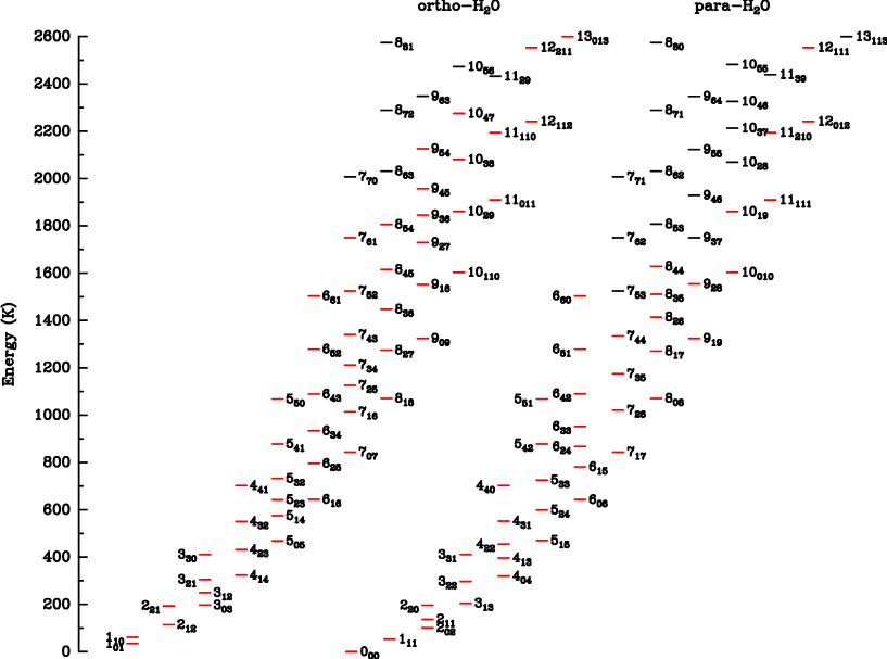
Figure 8: Rotational energy level diagram of the H₂O $v=0$ vibrational state showing in red the levels from which at least one absorption line is detected in VV 114 SW-s2.

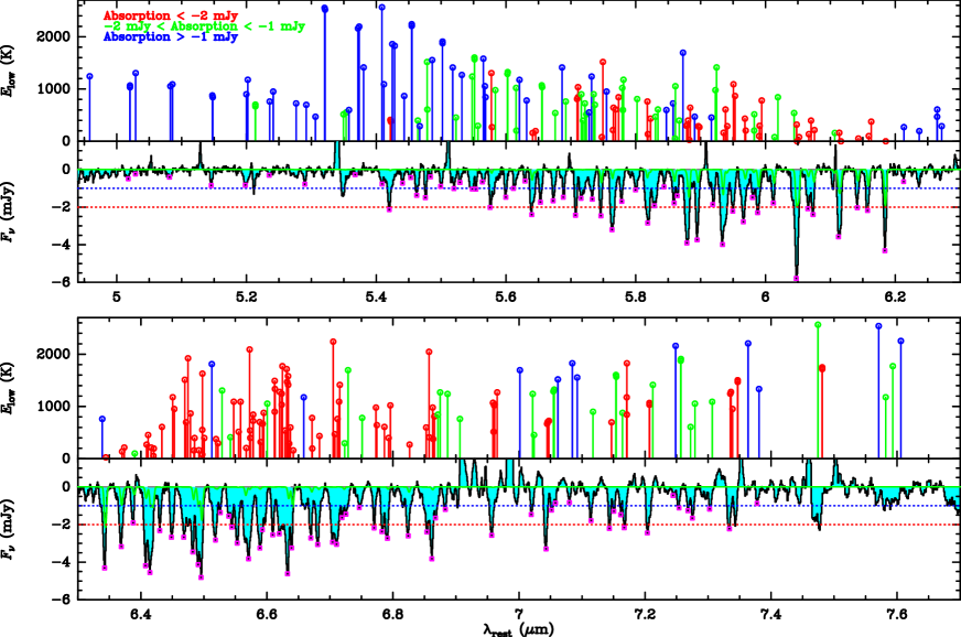
Figure 9: The H₂O $\nu_{2}=1-0$ band lines that contribute significantly to the features in the $5.0-7.7$ $\mu$m spectrum of VV 114 SW-s2. In the upper panels, the $E_{\mathrm{low}}$ values are plotted with vertical segments ending in circles, and are coloured according to the absorption strength of the spectral feature they belong to relative to the horizontal dotted lines in the lower panels. The magenta squares overplotted on the spectrum indicate the peak flux values for the 116 spectral features that are used to compare the band with model results (Fig. 4c-d).

Our fiducial model in Fig. 2 captures the general behaviour of the H₂O band. The contribution of the $W_{C}$ (Fig. 4c-d) is important for the low excitation lines lying beween $5.6$ and $6.8$ $\mu$m, but negligible on both ends of the band. We note that the MRS spectrum, with high quality for $\lambda_{\mathrm{rest}}<6.9$ $\mu$m, shows ripples at longer wavelengths where the measured peak absorption of the H₂O spectral features have thus larger uncertainties (Fig. 4d). Across the H₂O band (Fig. 2), there are still some spectral features that are unidentified or significantly underestimated. Among the former, the $6.313$ and $6.325$ $\mu$m adjacent features, the $6.660$ $\mu$m absorption in between the $7_{26}-7_{35}$ and $1_{11}-2_{20}$ lines, and the shoulders flanking the $2_{12}-3_{21}$ line at $6.826$ $\mu$m. The spectral features that are underestimated by more than 35% are: $5.321$ $\mu$m ($13_{112}-12_{211}$ & $13_{212}-12_{111}$), $5.440$ $\mu$m ($7_{25}-6_{24}$), $6.237$ $\mu$m ($3_{13}-2_{20}$), $6.265$ $\mu$m ($6_{16}-5_{23}$), and $7.378$ $\mu$m ($6_{33}-7_{44}$) (but the strength of the latter feature is relatively uncertain).

As indicated in the main text, the areas $A_{\mathrm{CO,H_{2}O}}$ are hard to constrain, specifically because of their dependence on the thickness of the absorbing shell and on the velocity field. There is a mismatch of $\sim 30$% between $A_{\mathrm{CO}}$ and $A_{\mathrm{H_{2}O}}$ in the $H_{C}$ (and thus between the predicted associated continua in Fig. 1g) that may be due to these dependences. The H₂O-to-CO abundance ratio in the $H_{C}$ is $\sim 1$, orders of magnitude higher than the typical values derived in cold molecular gas (e.g. Melnick et al. 2020). This is in line with expectations for hot (several hundred K) material, as in such environments icy grain mantles will have been vaporized and any atomic oxygen in the gas phase will have been converted to H₂O in high temperature neutral-neutral reactions with H₂. The mismatch in areas is also seen in the $W_{C}$, but in this case can be attributed to the different excitation of both species in more moderate environments, where CO will be more widespread than H₂O.

The H₂O $\nu_{1}=1-0$ and $\nu_{3}=1-0$ bands lie at $2.5-3.0$ $\mu$m, and the $\nu_{3}$ band is the strongest. This $\nu_{3}$ band is not detected in SW-s2. We have generated LTE models for it, using the same parameters as in our LTE models for the $\nu_{2}$ band in Fig. 4c-d but with a background radiation temperature of $T_{\mathrm{bck}}=1400$ K (Fig. 1g). If the absorbing H₂O gas were fully covering the $2.5-3.0$ $\mu$m continuum as well, the models indicate that strong absorption would be detected in the H₂O $\nu_{3}$ band; the lack of detection indicates that H₂O is covering $\lesssim 5$% of the $2.5-3.0$ $\mu$m continuum emission. Therefore, the nir continuum from SW-s2 is not related to the $4.4-8.0$ $\mu$m continuum associated with the CO $v=1-0$ and H₂O $\nu_{2}=1-0$ bands. This result is fully consistent with our model for the continuum in Fig. 1g, involving strong attenuation of the component that dominates the mid-IR $4.4-8.0$ $\mu$m emission (see also Appendix D).

Appendix D The mid-IR extinction

We show in Fig. 10 the extinction required to match the $T_{\mathrm{app}}$ values inferred in VV 114 SW-s2, assuming intrinsic blackbody emission with $T=550$ K (panel a) and 600 K (panel b). These blackbody curves have a slope across the CO band ($4.4-5.0$ $\mu$m) very different from $T_{\mathrm{app}}\sim 400$ K (green upper curves), which is the value inferred from the CO P-R asymmetry. After applying the extinction law by Indebetouw et al. (2005) and Chiar & Tielens (2006) with $\tau_{\mathrm{6\mu m}}^{\mathrm{ext}}=2.5-3$, the resulting reddened slopes (red curves) at $4.4-5.0$ $\mu$m approach the required steep values. Extinction also changes the slope across the H₂O band, with $T_{\mathrm{app}}\sim 500$ K at long wavelengths (blue curves). High values of $\tau_{\mathrm{6\mu m}}^{\mathrm{ext}}=2.5-3$, which attenuate the intrinsic continuum emission by $\sim 1$ dex, are needed to match the $T_{\mathrm{app}}$ values derived from the molecular bands.

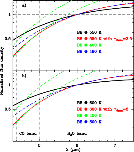
Figure 10: Effect of extinction on the mid-IR continuum slope. The broad black lines show the shape of a blackbody source with a) $T=550$ K, and b) $T=600$ K. The red curves indicate how the SED changes when the blackbody emission is affected by extinction with $\tau_{\mathrm{6\mu m}}^{\mathrm{ext}}=2.5-3$, using the extinction law derived by Indebetouw et al. (2005) and Chiar & Tielens (2006). The dashed green and blue curves are reference blackbodies at 400 and $480-500$ K.

Appendix E CO band profiles and the best-fit model

The continuum-normalized profiles of the CO $v=1-0$ lines up to $J=32$ are compared with predictions of our best-fit model in Fig. 11. The positions of the ¹³CO ro-vibrational lines are indicated in brown.

The model fit is globally satisfatory, but there are some significant discrepancies. First, the CO P(1) line is not fully reproduced, probably indicating the presence of additional cold gas along the line-of-sight to the continuum source that the $C_{C}$ does not account for. A probably related issue is that the absorption between CO P(8) and P(9) and between CO P(14) and P(15) are not fully reproduced (see also Fig. 2). These absorption are coincident with the rest position of the ¹³CO R(3) and P(3) lines, most likely indicating that the column density of the $C_{C}$ is underestimated. Finally, we note that the CO R(4)-R(13) lines are all underpredicted at central and redshifted velocities, but this effect is not seen in the P-branch counterpart. This is indicative of the complexity of the $W_{C}$, which most likely probes several components associated with the mid-IR source, and some of them could contribute with different absorption strengths in the two branches (Pereira-Santaella et al. 2023; García-Bernete et al. 2023).

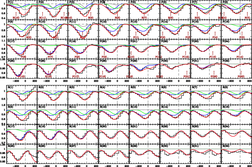
Figure 11: Continuum-normalized profiles of the CO $v=1-0$ lines up to $J=32$. The positions of the ¹³CO lines are indicated in brown. The best-fit model is overlaid in red, and the contribution by the individual components is also shown ($H_{C}$: blue, $W_{C}$: green, and $C_{C}$: gray). The abscissa axis is velocity in km s^-1 relative to the redshift inferred from the CO ($3-2$) line, $z=0.02013$.

Appendix F Estimating the BH mass from lifetime constraints

Eddington luminosity ($L_{\mathrm{Edd}}$) and BH mass ($M_{\mathrm{BH}}$) are equivalent through the standard relation $M_{\mathrm{BH}}=A\,L_{\mathrm{Edd}}$, where $A=3.0\times 10^{-5}\,M_{\odot}L_{\odot}^{-1}$. However, the actual luminosity $L$,

$$L\sim 10^{10}\exp\{\tau_{\mathrm{6\mu m}}^{\mathrm{ext}}-2.5\}\,L_{\odot},$$ (4)

will generally depart from $L_{\mathrm{Edd}}$, and we write

$$M_{\mathrm{BH}}=\frac{A}{\epsilon}\,L$$ (5)

where $\epsilon\equiv\frac{L}{L_{\mathrm{Edd}}}$. The mass accretion rate is given by

$$\dot{M}_{\mathrm{BH}}=\frac{L}{\eta c^{2}}$$ (6)

where $\eta$ is the radiative efficiency. We can also define $\eta_{\mathrm{Edd}}\equiv 0.1$, but the actual value of $\eta$ may also depart from $\eta_{\mathrm{Edd}}$. Using eqs. (5) and  (6),

$$\dot{M}_{\mathrm{BH}}=\frac{\epsilon}{A\,c^{2}\eta}M_{\mathrm{BH}}$$ (7)

with the solution

$$M_{\mathrm{BH}}(t)=M_{\mathrm{BH,0}}\exp\{t/t_{0}\},$$ (8)

where we have assumed that $\epsilon/\eta$ remains constant. The $e-$folding time is

$$t_{0}=\frac{A\,c^{2}\eta}{\epsilon}$$ (9)

To proceed further, we need $(i)$ the relationship between $\epsilon$ and $\eta$, and $(ii)$ the time constraint for the BH growth:

• The relationship derived by Watarai et al. (2000) for the “slim disk” model is used, which we re-write here as in Toyouchi et al. (2021):

  $$L=\cases{2}L_{\mathrm{Edd}}\left[1+\ln\left(\frac{\dot{M}_{\mathrm{BH}}}{2\dot{M}_{\mathrm{Edd}}}\right)\right]&(\mathrm{if}\,\,\dot{M}_{\mathrm{BH}}>2\dot{M}_{\mathrm{Edd}})\\ L_{\mathrm{Edd}}\left(\frac{\dot{M}_{\mathrm{BH}}}{\dot{M}_{\mathrm{Edd}}}\right)\mathrm{(otherwise)}{}$$ (10)

  where $\dot{M}_{\mathrm{Edd}}\equiv L_{\mathrm{Edd}}/(\eta_{\mathrm{Edd}}\,c^{2})$. The curve is shown in Fig. 12. $\epsilon\equiv\frac{L}{L_{\mathrm{Edd}}}$ flattens for $\dot{M}_{\mathrm{BH}}/\dot{M}_{\mathrm{Edd}}>2$ accounting for the low radiative efficiency at high accretion rates, but can attain values $\epsilon\sim 10$. Similar excesses of $L$ over $L_{\mathrm{Edd}}$ together with beaming effects are the basis for the interpretation of most ultraluminous X-ray sources (ULXs) as super-Eddington accreting stellar BHs or neutron stars in binary systems (XRBs, e.g. Begelman et al. 2006; Poutanen et al. 2007; King 2008). The above relationship can be rewritten in terms of $\epsilon$ and $\eta$:

  $$\epsilon=\cases{2}\left[1+\ln\left(\frac{\epsilon\,\eta_{\mathrm{Edd}}}{2\eta}\right)\right]&\mathrm{(if\,\,\epsilon\,\eta_{\mathrm{Edd}}>2\eta)}\\ \frac{\epsilon\,\eta_{\mathrm{Edd}}}{\eta}\rightarrow\eta=\eta_{\mathrm{Edd}}\mathrm{(otherwise)}{}$$ (11)

• The fiducial time $t$ required to attain the current mass is (Section 4.3)

  $$t\sim 10\,\mathrm{Myr},$$ (12)

  with an uncertainty of a factor $\sim 2$. We estimate the $e-$folding time $t_{0}$ using eq. (5) and our result for the luminosity $L$ in eq. (4),

  $$M_{\mathrm{BH}}(t)=\frac{3\times 10^{5}\,M_{\odot}}{\epsilon}\exp\{\tau_{\mathrm{6\mu m}}^{\mathrm{ext}}-2.5\}$$ (13)

  Using now eq. (8), and assuming an initial BH seed with mass $M_{\mathrm{BH,0}}\sim 100\,M_{\odot}$, we obtain

  $$t=t_{0}\left[\ln\left(\frac{3\times 10^{3}}{\epsilon}\right)+(\tau_{\mathrm{6\mu m}}^{\mathrm{ext}}-2.5)\right]$$ (14)

  We expect high accretion rates with $\epsilon$ in the range $[1,10]$, and then

  $$t=t_{0}\left[(5.7-8)+(\tau_{\mathrm{6\mu m}}^{\mathrm{ext}}-2.5)\right],$$ (15)

  where the values $5.7$ and $8$ correspond to $\epsilon=10$ and 1, respectively. In view of this result and for simplicity, we can write the time constraint in eq. (12) in terms of the $e-$folding time as

  $$t_{0}=\frac{Ac^{2}\eta}{\epsilon}\sim 2^{+2}_{-1}\,\mathrm{Myr}.$$ (16)

Figure 12: Adopted relationship between $\epsilon\equiv L/L_{\mathrm{Edd}}$ and the mass accretion rate onto the BH relative to the Eddington value; as derived by Watarai et al. (2000). Note that $\dot{M}_{\mathrm{Edd}}$ is here defined as $10\times$ the value defined in Watarai et al. (2000).

With these prescriptions, we first note that the second solution of eq. (11) and the time constraint eq. (16) are not compatible. Since in this case $\eta=\eta_{\mathrm{Edd}}=0.1$, eq. (16) gives

$$\epsilon=\frac{Ac^{2}\eta_{\mathrm{Edd}}}{t_{0}}=45.5\left(\frac{t_{0}}{1\,\mathrm{Myr}}\right)^{-1}$$ (17)

where we have used that $A\,c^{2}=455$ Myr. However, this solution is only valid for $\epsilon\,\eta_{\mathrm{Edd}}<2\eta$, that is, for $\epsilon<2$ ($t_{0}\geq 23$ Myr).

We then resort to the first solution of eq. (11) and (16), which give

$$t_{0}=\frac{Ac^{2}\eta_{\mathrm{Edd}}}{2\exp\{\epsilon/2-1\}},$$ (18)

which is used to evaluate $\epsilon$:

$$\epsilon=2\left[\ln\left(\frac{Ac^{2}\eta_{\mathrm{Edd}}}{2t_{0}}\right)+1\right]=8.2-2\ln t_{0},$$ (19)

where $t_{0}$ is in Myr. Inserting this constraint in eqs. (4) and (5), we obtain an estimate of the mass of the BH:

$$M_{\mathrm{BH}}=\frac{A}{\epsilon}\,L\sim\frac{3.7\times 10^{4}\,M_{\odot}}{1-0.244\ln t_{0}}\,\exp\{\tau_{\mathrm{6\mu m}}^{\mathrm{ext}}-2.5\},$$ (20)

which is an IMBH as long as $t_{0}<15$ Myr. For the fiducial $t_{0}\sim 2$ Myr, $M_{\mathrm{BH}}\sim 4.5\times 10^{4}\,M_{\odot}$, and the current mass accretion rate is then

$$\dot{M}_{\mathrm{BH}}=\frac{M_{\mathrm{BH}}}{t_{0}}\sim 2.3\times 10^{-2}\exp\{\tau_{\mathrm{6\mu m}}^{\mathrm{ext}}-2.5\}\,\,M_{\mathrm{\odot}}\,\mathrm{yr^{-1}},$$ (21)

with $\eta\sim 2.8\times 10^{-2}$ and $\dot{M}_{\mathrm{BH}}/\dot{M}_{\mathrm{Edd}}\sim 25$.