Enhancement of Goos-Hänchen shifts in graphene through Fizeau drag effect

Abstract

We investigate the Goos-Hänchen shifts in reflection for a light beam within a graphene structure, utilizing the Fizeau drag effect induced by its massless Dirac electrons in incident light. The magnitudes of spatial and angular shifts for a light beam propagating against the direction of drifting electrons are significantly enhanced, while shifts for a beam co-propagating with the drifting electrons are suppressed. The Goos-Hänchen shifts exhibit augmentation with increasing drift velocities of electrons in graphene. The impact of incident wavelength on the angular and spatial shifts in reflection is discussed. Furthermore, the study highlights the crucial roles of the density of charged particles in graphene, the particle relaxation time, and the thickness of the graphene in manipulating the drag-affected Goos-Hänchen shifts. This investigation offers valuable insights for efficiently guiding light in graphene structures under the influence of the Fizeau drag effect.

I Introduction

The optical phenomenon known as the Fizeau drag effect was first elucidated in 1851 by Armand Fizeau Fizeau (1851) and was later verified for light propagating in flowing water Banerjee et al. (2022); Davuluri and Rostovtsev (2012); Kuan et al. (2016). Under this effect, the speed of light can be modified when it is propagating in a moving medium. This effect arises when a moving optical element, such as a moving mirror or transparent material, partially entrains a medium. In the Fizeau experiment, light was directed through a tube containing a flowing liquid. The light beam was split, with one part moving in the direction of the liquid’s flow and the other against it. Upon recombining the two beams, interference fringes were observed. The experiment demonstrated that the motion of the medium through which light traveled influenced its speed. The beam moving with the flow of the liquid resulted in a slight increase in speed, while the beam moving against the flow led to a slight decrease in speed. This differential effect caused a shift in the interference fringes.

By utilizing the high electron mobility in graphene Geim and Novoselov (2007); Geim (2009) and the slow plasmon propagation of its massless Dirac fermions, Dong et al. Dong et al. (2021) and Zhao et al. Zhao et al. (2021) recently demonstrated experimentally Fizeau drag effect for graphene plasmons. They observed that the Dirac electrons in graphene possess the ability to effectively drag surface plasmons along their direction of propagation, a phenomenon highlighted by the observed wavelength change in these modes.

On the other hand, when light interacts with dielectric interfaces, reflection and transmission occur Saleh and Teich (2019). In the case of total internal reflection at the interface between two media, the reflected beam deviates laterally from the position predicted by geometrical optics. This lateral shift is known as the Goos-Hänchen (GH) shift Goos and H¨anchen (1947) and arises due to the phase shift between the reflected and transmitted beams Wang et al. (2008a, 2013a); Wu et al. (2019a). In this phenomenon, each plane-wave component undergoes a distinct phase change, causing the reflected beam, resulting from the superposition of these components, to experience a lateral displacement. Furthermore, the different reflective coefficients of each plane wave component contribute to an angular change Wan and Zubairy (2020). Widely applicable in angle measurements Yallapragada et al. (2016), beam splitters Song et al. (2012), sensors Wang et al. (2008b), and optical switches Wang et al. (2013b), the GH shift has been extensively studied in various media and structures, including metal and dielectric slabs Wan and Zubairy (2020); Li (2003), optical cavities or waveguides Kandammathe Valiyaveedu et al. (2018); Zhu et al. (2016), photonic crystals Soboleva et al. (2012); Din et al. (2022), metamaterials Wu et al. (2019b); Yallapragada et al. (2016), optomechanical systemsUllah et al. (2019); Khan et al. (2020), atomic media Wang et al. (2008a); Radmehr et al. (2016), surface plasmon resonance structures Yin et al. (2004); Salasnich (2012), graphene Li et al. (2014); Chen et al. (2017); Song et al. (2012); Wu et al. (2017); Grosche et al. (2016) and other 2D materials Shah (2022); Jahani et al. (2023). GH shifts in geometries containing graphene can be efficiently tuned by graphene, depending on its remarkable properties, such as adjusting its carrier density through the applied gate voltage Cheng et al. (2014); Zeng et al. (2017), varying its number of layers or thickness Li et al. (2014); Chen et al. (2017), using different substrates on which it is deposited Blake et al. (2007); Novoselov et al. (2012), and varying the direction of polarization of incident light Li et al. (2014). These investigations span both the fundamental understanding and practical aspects of the GH shift.

The GH shift, though typically a tinny effect, has significant implications in various optical applications such as precision measurement and interferometry. As a result, an important issue is studying how to improve the shift. We realize that one such way could be the implementation of relativistic effects in graphene caused by its fast-moving, massless Dirac electrons. They can effectively drag light along or against their propagation direction, and the resulting shifts for light can be either enhanced or suppressed. To our knowledge, no such study has been reported in the literature. Therefore, in this paper, we employ the Fizeau drag effect associated with the propagation of light through graphene due to its drifting charge carriers and manipulate the resulting GH shifts of light.

We explore the dependencies of the drag-affected GH shifts on the thickness of two-dimensional (2D) graphene sheet, its carrier density, and the incident wavelength. The enhancement of GH shifts is observed in this 2D material. Our findings reveal that depending upon the direction of propagation of the incoming light, the angular and spatial shifts of the reflected beam are significantly amplified or suppressed by the inclusion of Fizeau drag due to the swift motion of electrons in graphene. This dependency is demonstrated across various drift velocities of electrons in graphene. This study presents an efficient platform for guiding light through graphene in its current-carrying state.

The paper is organized as follows. In Sect. II, we define the geometry and revise the Fizeau drag effect based on the special relativity. Subsequently, we present the analytical expressions for the description of GH shifts. Then we present expressions for describing the transformations from a stationary frame to a moving frame, as well as for the optical response of graphene. The results are presented and discussed in Sect. III and the last section (Sect. IV), summarizes the results.

II Model and Expressions for GH Shift with Fizeau Drag

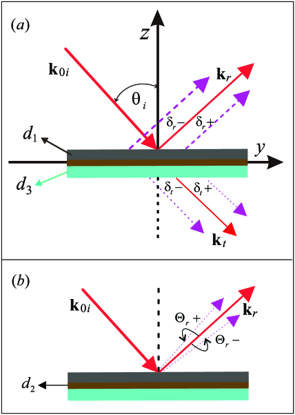
Figure 1: Three-layered structure for the investigation of GH shifts in reflection for a light beam under the effect of Fizeau drag. A graphene sheet of thickness $d_{2}$ is deposited between two dielectric media of thicknesses $d_{1}$ and $d_{3}$. ${\bf k}_{0i}$ is the wave vector of the incident beam, ${\bf k}_{r}$ is its reflected part, and ${\bf k}_{t}$ is its transmitted part. $\theta_{i}$ denotes the angle of incidence of the light beam. ($a$) shows a schematic of the spatial shifts in reflection ($\delta_{r}$) while the angular shifts ($\Theta_{r}$) are shown in ($b$).

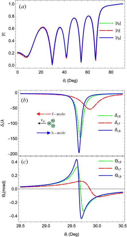
Figure 2: (a) Reflection coefficients, (b) spatial and (c) angular GH shifts of the reflected wave as a function of incident angle $\theta_{i}$. The dashed-dotted green curves correspond to the drag-free light case, $k_{g}$ (in graphene), while the red dashed and solid blue curves correspond to the coefficients and shifts for drag-affected forward $k_{g,f}(\omega)$ and backward $k_{g,b}(\omega)$ modes. Notably, the angular and spatial shifts are suppressed for a beam of light propagating along the drifting electrons, whereas they are enhanced for a beam of light moving against the drifting electrons. The directions of propagation of the drifting electrons (shown as the small green circles) and incoming light beam are indicated by the arrows. For the drag-affected case, we assume $v_{D}=0.35v_{F}$ in graphene.

The geometry depicted in Fig. 1 illustrates our model for investigating GH shifts of a light beam under the influence of the Fizeau drag effect in graphene. A linearly polarized light ${\bf k}_{0i}$ impinges on a three-layered structure at an incident angle $\theta_{i}$ with the $z$-axis. The three layers consist of a graphene sheet with relative electric permittivity $\varepsilon_{2}$ positioned between a substrate with relative dielectric constant $\varepsilon_{3}$ and an upper medium with relative electric permittivity $\varepsilon_{1}$. The parameters $d_{1}$, $d_{2}$, and $d_{3}$ represent the thicknesses of the top medium, the graphene layer, and the substrate, respectively. In this context, $\delta_{r}$ denotes the spatial GH shift, and $\Theta_{r}$ represents the angular shift of the reflected wave, with $\pm$ indicating the corresponding positive and negative shifts. Vectors ${\bf k}_{r}$ and ${\bf k}_{t}$ denote the reflected and transmitted portions of the incident light. Further insights into such a three-layered model can be found in previous works discussing GH shift phenomena Wang et al. (2008a); Song et al. (2012); Din et al. (2022)

We aim to explore spatial and angular shifts in the depicted geometry by incorporating the influence of Fizeau drag caused by Dirac electrons in graphene. In subsequent sections, we outline the Fizeau drag effects of Dirac electrons in graphene on the incident light. Subsequently, we provide expressions for the GH shifts in both reflection and transmission.

II.1 Fizeau drag in graphene and the resulting expressions for drag-affected GH shifts

We make the assumption that the Fizeau drag that affects the incident light is solely a result of the drifting electrons in graphene. These drifting electrons are considered to propagate along the positive $y$-axis. To explore the GH shifts in the current-carrying state, we begin our analysis with Lorentz transformations applied to various physical quantities of graphene Borgnia et al. (2015); Dong et al. (2021)

$$\omega_{0}=\gamma(\omega-v_{D}k_{g}),$$ (1)

$$k_{g,0}=\gamma(k_{g}-\frac{v_{D}}{c^{2}}\omega),$$ (2)

$$n_{0}=\frac{1}{\gamma}n~{},$$ (3)

where $\omega$ represents the frequency of the incident light, $k_{g}$ is the wave vector of light in graphene, $n$ is the charge density, and $v_{D}$ denotes the drift velocity of the charged particles in graphene. The subscript “0” designates the quantities measured in the frame moving with velocity $v_{D}$, and $\gamma=(1-v_{D}^{2}/v_{F}^{2})^{-1/2}$ denotes the Lorentz factor Dong et al. (2021). Given our assumption that graphene possesses free electrons and an associated electric current, the effective relative optical permittivity $\varepsilon_{2}(\omega)$ of graphene, for a monochromatic light with angular momentum $\omega$, can be derived from its optical conductivity $\sigma(\omega)$ using Maxwell’s equations as Saleh and Teich (2019)

$$\varepsilon_{2}(\omega)=\frac{\varepsilon_{1}+\varepsilon_{3}}{2}+\frac{i\sigma(\omega)}{\omega\varepsilon_{0}}~{},$$ (4)

where $\varepsilon_{0}$ represents the vacuum permittivity. An essential parameter for an accurate depiction of the dielectric properties of graphene is its optical conductivity. This quantity is contingent on both the incoming frequency and the in-plane wave vector. Notably, the energy–momentum relationship for electrons in graphene is linear for energies below $1eV$, as opposed to being quadratic. Consequently, the low-energy conductivity of graphene encompasses two components: intraband and interband contributions. The graphene conductivity, derived from the Kubo formula Gusynin et al. (2006) or the random phase approximation Platzman and Wolff (1973), is expressed as $\sigma(\omega)=\sigma_{\text{intra}}(\omega)+\sigma_{\text{inter}}(\omega)$. These contributions arise from intraband electron-phonon scattering and interband electron transitions, given by Hanson (2008)

$$\sigma_{\mathrm{intra}}(\omega) =\frac{e^{2}\epsilon_{F}}{\pi\hbar^{2}}\frac{i}{\omega+i\tau^{-1}}~{},$$ (5)

$$\sigma_{\mathrm{inter}}(\omega) =\frac{e^{2}}{4\hbar}\bigg{\{}\vartheta(\hbar\omega-2\epsilon_{F})+\frac{i}{\pi}\log\left|\frac{\hbar\omega-2\epsilon_{F}}{\hbar\omega+2\epsilon_{F}}\right|\bigg{\}}~{}.$$

Here, $\epsilon_{F}=\hbar v_{F}k_{F}$ represents the Fermi energy, where $k_{F}=\sqrt{\pi n}$ is the Fermi wave vector, and $v_{F}=c/300$ is the Fermi velocity of the charged particles. The parameter $\tau$ denotes the relaxation time of the charge carriers with density $n$, and $\vartheta$ is the Heaviside function. It is important to note that the presented formulas are applicable for highly doped or gated graphene, specifically when $\mu\gg k_{B}T$. In the long wavelength and high doping limit, i.e., $\hbar\omega\ll\epsilon_{F}$, the interband contributions become negligible, and the intraband term dominates, defining the total conductivity of graphene.

We will see that the normal component of the incident light corresponding to the graphene sheet is

$$k^{z}_{g}(\omega)=\sqrt{k_{g}^{2}(\omega)-k^{2}_{y}}~{},$$ (6)

where $k_{g}=\sqrt{\varepsilon_{2}(\omega)}k_{0}$ is the wave vector propagating with velocity $v$ in graphene and $k_{y}$ the $y$-component of the wave vector $k_{0}$. If we consider the Fizeau effect due to drifting electrons in graphene, the phase velocity of the wave becomes

$$v_{0}=v\pm v_{D}F(\omega)~{},$$ (7)

where the $+$ and $-$ signs stand for a wave propagating along and against the drifting electrons in graphene, respectively. We call the former the forward (f) mode and the latter as backward (b) mode. $F(\omega)$ in Eq. (7) is the drag coefficient of graphene and is obtained as

$$F(\omega)=\frac{n_{g2}(\omega)}{n_{2}(\omega)}-\frac{1}{n^{2}_{2}(\omega)}.$$ (8)

where $n_{2}(\omega)=\sqrt{\epsilon_{2}(\omega)}$ represents the refractive index of graphene and $n_{g2}(\omega)=n_{2}(\omega)+\omega\frac{\partial n_{2}(\omega)}{\partial\omega}$ is its group index. Rewriting Eq. (7) in terms of wave vectors and applying the transformations given by Eqs. (1) and (2), we obtain the following expression:

$$\frac{\gamma(\omega-v_{D}k_{g}(\omega))}{k_{g,0}}-\frac{\gamma\omega c^{2}}{c^{2}k_{g,0}+\gamma\omega v_{D}}\mp v_{D}F(\omega)=0~{}.$$ (9)

Notice that $k_{g,0}$ becomes $k_{g,b}(\omega)$ for the upper sign and $k_{g,f}(\omega)$ for the lower sign, the Fizeau drag-affected wave vectors of the backward mode and forward mode, respectively. Solving these equations, we get a quadratic equation in $k_{g,f}$ and $k_{g,b}$ for each mode whose solution is

$$k_{g,f}(\omega) =\frac{-\gamma c^{2}k_{g}\pm v_{D}\gamma\omega F+\gamma\sqrt{k^{2}_{g}c^{4}-2c^{2}v_{D}\omega k_{g}F+4c^{2}\omega^{2}F+v_{D}^{2}\omega^{2}F}}{2c^{2}F}~{}$$ (10)

$$k_{g,b}(\omega) =\frac{\gamma c^{2}k_{g}-v_{D}\gamma\omega F\pm\gamma\sqrt{k^{2}_{g}c^{4}-2c^{2}v_{D}\omega k_{g}F+4c^{2}\omega^{2}F+v_{D}^{2}\omega^{2}F}}{2c^{2}F}~{}.$$ (11)

The $y$ component of this drag-affected wave vector becomes $k_{y,0}=k_{g,0}\sin\theta_{i}$. Additionally, the Fermi energy in the current-carrying graphene channel is modified to $\epsilon_{F}=\hbar v_{F}\sqrt{\pi n_{0}}$, where $n_{0}$ is determined by the transformation given in Eq. (3). Substituting these values into the expressions for the GH shifts, we obtain the desired results for spatial and angular shifts of light under the Fizeau drag effect.

II.2 General expressions for GH shifts

The incident wave on the geometry presented in Fig. 1 undergoes partial transmission and partial reflection through the substrate layer to reach the graphene. The wave can be expressed as $k_{0x}(y,0)=\frac{1}{\sqrt{2\pi}}\int f(k_{y})e^{ik_{y}y}dk_{y}$ in the plane $z=0$, where $k_{0y}=k_{0}\sin\theta_{i}$ is its $y$ component and $f(k_{y})$ is defined by $f(k_{y})$=$\frac{\beta_{y}}{\sqrt{2}}\exp\{-\beta^{2}_{y}(k_{y}-k_{y0})^{2}/4\}$ where $\beta$ represents the half width of the incident wave and $\beta_{y}=\beta\sin\theta_{i}$ is its $y$ component. Assuming that the incident wave has a sufficiently large width, that is, $\Delta k\ll k$, the Goos-Hänchen shifts for the reflected and transmitted beams can be obtained using stationary phase theory Wang et al. (2008a); Cheng et al. (2014), which has been demonstrated to be accurate for structures containing graphene Li et al. (2014); Song et al. (2012). To facilitate this, we start the analysis with the standard characteristic matrix approach Wang et al. (2008a, 2013a), where the input and output of the electric field propagating through each medium in the structure are related via the transfer matrix.

$$M_{j}(k_{y},\omega,d_{j})=\left(\begin{array}[]{cc}\cos(k^{z}_{j}d_{j})&i\sin(k^{z}_{j}d_{j})/\alpha_{j}\\ i\alpha_{j}\sin(k^{z}_{j}d_{j})&\cos(k^{z}_{j}d_{j})\\ \end{array}\right)~{},$$ (12)

where $\alpha_{j}=k^{z}_{j}/k_{0}$, $k^{z}_{j}=\sqrt{\varepsilon_{j}k^{2}-k^{2}_{y}}$ is the z-component of the incident wave vector $k_{0}$ in medium $j$ such that $k_{0}=2\pi/\lambda$ is the wave vector in vacuum. $d_{j}$ is the thickness of the $j$th medium where $j$=1,2,3. For the three-layered nanostructure in our model, the total transfer matrix is

$$X(k_{y},\omega,d_{j})=M_{1}(k_{y},\omega,d_{1})M_{2}(k_{y},\omega,d_{2})M_{3}(k_{y},\omega,d_{3}).$$ (13)

The reflection (transmission) coefficient $r(k_{y},\omega,\theta_{i})=|r|e^{i\varphi_{r}}$ ($t(k_{y},\omega,\theta_{i})=|t|e^{i\varphi_{t}}$), where $\varphi_{r(t)}$ denotes the phase of the reflection (transmission) coefficient, can be determined as

$$r(k_{y},\omega,\theta_{i})=\frac{\alpha_{0}(X_{22}-X_{11})-(\alpha^{2}_{0}X_{12}-X_{21})}{\alpha_{0}(X_{22}+X_{11})-(\alpha^{2}_{0}X_{12}+X_{21})}~{},$$ (14)

$$t(k_{y},\omega,\theta_{i})=\frac{2\alpha_{0}}{\alpha_{0}(X_{22}+X_{11})-(\alpha^{2}_{0}X_{12}+X_{21})}~{},$$ (15)

where $\alpha_{0}=k^{z}_{0}/k_{0}$ such that $k^{z}_{0}$ is the z-component of the wave vector $k_{0}$ in vacuum and $X_{ij}$ are the elements of transfer matrix given by Eq. (13). Having calculated $r(k_{y},\omega,\theta_{i})$ and $t(k_{y},\omega,\theta_{i})$, the lateral shifts (GH shifts) for a monochromatic beam of wavelength $\lambda$ can be calculated by using stationary phase theory Wang et al. (2008a); Cheng et al. (2014). The GH shift in reflection (transmission) is $S_{r(t)}=-\frac{\lambda}{2\pi}D_{r(t)}$, where

$$D_{r(t)}=\frac{\partial\varphi_{r(t)}}{\partial\theta_{i}}=\frac{1}{|r|(|t|)}\frac{\partial|r|(|t|)}{\partial\theta_{i}}+i\frac{\partial\varphi_{r(t)}}{\partial\theta_{i}}.$$ (16)

However, we are interested in spatial $\delta_{\lambda}$ and angular $\Theta_{\lambda}$ GH shifts independently that contribute to the total GH shifts via $S_{\lambda}$=$\delta_{\lambda}+l\Theta_{\lambda}$ Aiello et al. (2009), and $l$ represents the distance from the origin of the point at which the total beam shift is observed. The spatial and angular shifts in reflection and transmission are given, respectively, by  Aiello et al. (2009); Cheng et al. (2014)

$$\delta_{r}=\frac{\lambda}{2\pi}\mathrm{Im}[D_{r}]~{},\delta_{t}=\frac{\lambda}{2\pi}\mathrm{Im}[D_{t}]~{},$$ (17)

$$\Theta_{r}=-\frac{\theta^{2}_{0}}{2|r|}\mathrm{Re}[D_{r}]~{},\Theta_{t}=-\frac{\theta^{2}_{0}}{2|t|}\mathrm{Re}[D_{t}]~{}.$$ (18)

In the above expression, $\theta_{0}=2\lambda/w_{0}$ is the angular spread of the beam with $w_{0}$ its waist, $\mathrm{Re}$ ($\mathrm{Im}$) is the real (imaginary) part of the quantity. Notice that at this stage, we do need to substitute the Fizeau effect corrections into the expressions for the GH shifts so that we obtain the desired results for spatial and angular shifts for light. For the convenience of the reader, the modified expressions are provided in the appendix.

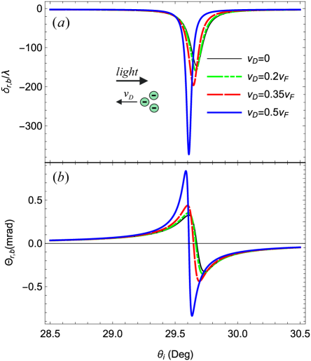
Figure 3: Variations of (a) the spatial and (b) angular GH shifts in reflection for the backward $k_{g,b}(\omega)$ mode with different drift velocities of the charged particles in graphene. The inset arrows indicate the directions of propagation of the drifting electrons (shown as the small green circles) and incoming light beam. The altering of the magnitudes as well as peak positions of the curves originate from the impact of the drag coefficient. Notice that the GH shifts of the backward mode increase noticeably with $v_{D}$ while the shifts for forward mode vary only slightly, and are not shown here.

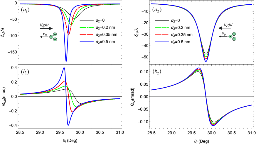
Figure 4: (a) Spatial and (b) angular GH shifts in reflection for the (1) backward $k_{g,b}(\omega)$ mode and (2) forward $k_{g,f}(\omega)$ modes as a function of $\theta_{i}$ with different thicknesses of the graphene sheet $d_{2}$. The magnitudes of GH shifts for both modes are noticeably enhanced with increasing $d_{2}$. The dependence of the GH shifts to $d_{2}$ comes from the trigonometric function of $d_{2}$ value in the transfer matrix. Similarly, the peaks of the curves indicate that the angle of TIR is slightly shifted towards lower incident angles with increasing $d_{2}$. The numerical results are obtained for $v_{D}=0.3v_{F}$, $n$=1$\times 10^{12}$cm^-2 and $\lambda$=600 nm.

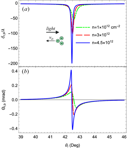
Figure 5: (a) Spatial and (b) angular GH shifts in reflection for the backward $k_{g,b}(\omega)$ mode as a function of $\theta_{i}$ with different charge densities $n$ in graphene. We have used $v_{D}=0.3v_{F}$, $d_{2}$=0.5 nm, and $\lambda$=580 nm. The GH peaks increase by increasing the electron density. We have found that the curves overlap in the case of forward mode.

III Numerical results and discussions

In this section, we present numerical results for the spatial and angular shifts of the reflected part of the light beam in our model under the Fizeau effect. We assume the carrier density in graphene to be $n=1\times 10^{12}$ cm^-2, and the relaxation time $\tau=10$ fs. The thicknesses of the different media in the structure are taken as $d_{1}=d_{3}=2.5\mu$m and $d_{2}=0.5$ nm. The waist of the incident beam is set to $w_{0}=1$ mm Wu et al. (2017), and the incident wavelength is $\lambda=600$ nm unless otherwise stated. The relative dielectric constants for the media above and below graphene are assumed to be $\varepsilon_{1}=4$ and $\varepsilon_{3}=3$ with $\varepsilon_{0}$ being the vacuum permittivity throughout this work.

Here we explain how to solve the sets of equations mentioned above. We start with Eq. (5) since the optical properties of graphene are strongly dependent on its conductivity $\sigma(\omega)$. We then substitute this expression into Eq. (4) and calculate the dielectric function of graphene. The dispersion characteristics of light propagating in graphene are obtained through $k_{g}=\sqrt{\varepsilon_{2}(\omega)}k_{0}$ and its normal component is obtained as in Eq. (6). At this stage, we are dealing with a normal graphene channel. To include the Fizeau effect, we make the transformation (1)-(3) to analyze the optical properties of graphene in the current-carrying state. Then, we consider the interaction of light with the structure. Depending upon the direction of propagation, the phase velocity of the incoming light is modified through Eq. (7). Making use of Eq. (9), we finally calculate the drag-affected wave numbers of light co- and counter-propagating with the drifting electrons in graphene by utilizing Eqs. (10) and (11). Subsequently, we calculate the transfer matrix of each medium in the geometry by using Eq. (12). However, the transfer matrix of the current-carrying graphene channel is modified as given in the appendix [Eq. (19)]. The reflection coefficient of light is obtained from Eq. (14) through Eq. (13). Finally, the spatial and angular shifts for the incoming light are calculated from Eqs. (17) and (18).

To initiate our analysis, we compare the results obtained for the GH shift of the reflected beam without drag and under the Fizeau drag effect. One of the three media is current carrying channel of graphene and is greatly modified as compared to a current-free graphene case. The comparison is presented in Fig. 2, where we illustrate (a) the reflection coefficients (b) spatial shifts, and (c) angular reflection shifts as functions of the incident angle $\theta_{i}$. For the drag-affected GH shifts, we assume the drift velocity of the electrons in graphene to be $v_{D}=0.35v_{F}$. We find that the reflection coefficients are almost overlapping for the two cases, forward and backward waves because of its small magnitude that only varies between 0 and 1. The difference becomes clear in the case of GH shifts where the magnitudes are very high. The oscillation of the reflection coefficients originates from the trigonometric function of $k_{j}d_{j}$ in the transfer matrix.

The dashed-dotted green curves depict the spatial $\delta_{r,0}/\lambda$ and angular $\Theta_{r,0}$ shifts of light without the Fizeau drag effect, i.e., $k_{g}$ in graphene. In comparison, we observe that the angular and spatial shifts for a light beam propagating along the direction of drifting electrons are significantly reduced, while those for a light beam propagating against the drifting electrons are markedly amplified. The modifications stem from the new momentum wave vectors in 2D graphene sheets. The charge carriers acquire finite drift velocity which affects the dispersion characteristics of the interacting light. This observation aligns well with the experimental outcomes in Refs. Dong et al. (2021); Zhao et al. (2021) on the Fizeau drag of surface plasmons due to Dirac electrons in graphene. In those experiments, it was observed that the wavelength of surface plasmons co-propagating with the charge carriers in the current-carrying graphene channel increased, while that of the counter-propagating plasmon decreased.

In our proposed structure, the Fizeau drag due to Dirac electrons in graphene also results in an enhancement and reduction of the wave numbers of the backward and forward modes. Consequently, the curves for GH shifts of drag-free light in our model lie between those for the forward mode and the backward mode. This implies that GH shifts for a light beam under Fizeau drag are direction-dependent. This directional dependence will be further elucidated when wavelength dependence of the GH shifts of light beam interacting with the given geometry is analyzed.

The point in Fig. 2 (b) where the magnitudes of the spatial shifts of the three modes are maximum corresponds to the critical angle at which the phenomenon of total internal reflection (TIR) occurs, which happens to be around 29.7^∘ in our studied structure. The angular shifts are also found to be maximum at the TIR angle, as shown in Fig. 2 (c). In addition to the magnitudes of the spatial and angular shifts, the peaks of the shifts also exhibit slight shifts toward higher (lower) incident angles for the forward (backward) mode.

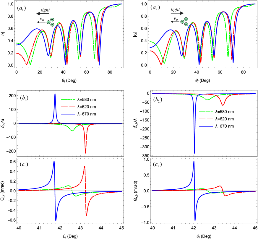
Figure 6: Dependence on the angle of incidence of the (a) reflection coefficient, (b) spatial and (c) angular GH reflection shifts of (1) the forward $k_{g,f}(\omega)$ mode and (2) backward $k_{g,b}(\omega)$ mode. The three different curves correspond to different incident wavelengths $\lambda$ of incoming light. The angle dependence of the GH peaks is no longer linear in terms of wavelength. We set $v_{D}=0.35v_{F}$, $d_{2}$=0.5 nm and $n$=1$\times 10^{12}$cm^-2.

To further explore the impact of the Fizeau drag on GH shifts, we plot the spatial and angular shifts of the forward and backward modes with different drift velocities $v_{D}$ of the electrons in graphene in Fig. 3. The drift velocity of the electrons can be adjusted by applying a direct current (dc) from a source Dong et al. (2021). The GH shifts are depicted with three different drift velocities of the charged particles, as indicated. We observe that the magnitudes of both the spatial and angular shifts are significantly magnified with increasing $v_{D}$ for both the counter- and co-propagating modes. This increase is independent of the initial magnitudes because the changes in the forward mode are smaller compared to those in the backward mode, but the increase with $v_{D}$ is the same for both. Similarly, the angle at which TIR occurs shifts to lower incident angles with increasing $v_{D}$. It is evident that any of the curves in Fig. 3 overlaps with the corresponding green curve in Fig. 2 at $v_{D}=0$. This demonstrates that the application of Fizeau drag can significantly affect GH shifts of light and should be considered when guiding light through graphene or other 2D materials of interest in current-carrying state.

In our proposed geometry, the Fizeau drag-affected GH shifts also strongly depend on the effective thickness $d_{2}$ of the graphene sheet. The thickness of graphene can be varied by considering ripples or wrinkles on it. This dependence is shown in Fig. 4 for three different thicknesses of the graphene layer, as indicated in the figure. We observe that the magnitudes of GH shifts for the forward and backward reflected modes are significantly enhanced with increasing $d_{2}$. Similarly, the curve peaks indicate that the TIR angle is slightly shifted towards lower incident angles as the intensity increases $d_{2}$. This variation is independent of the propagation direction, as the spatial and angular shifts of both modes are equally enhanced with the increasing thickness of the graphene sheet. Moreover, the angle of TIR is the same for both modes. These results are in good agreement with an experimental study Li et al. (2014), in which GH shifts were shown to increase with the effective layer thickness of graphene.

The GH reflection shifts under the effect of Fizeau drag vary in a similar manner as in Fig. 4 with increasing the number electron density $n$ of the charged particles in graphene. This is shown in Fig. 5 with three different number densities. We find that both spatial and angular shifts of the forward mode increase with increasing $n$ from 1 – 4.5 $\times$10¹²cm^-2 as shown in Fig. 5 (a) and (b). We also see that the angle of TIR is slightly shifted toward low incident angles with increasing $n$ for both spatial and angular shifts of the backward modes. This is in agreement with previous work by Cheng et al. Cheng et al. (2014) where the GH shifts were shown to decrease with decreasing Fermi energy. The Fermi energy in graphene varies with the number density as $\epsilon_{F}=\hbar v_{F}\sqrt{\pi n}$ and $n$ is further modified by Eq. (3) to account for the Fizeau effect in our studied structure.

The profiles of GH shifts under the effect of Fizeau drag exhibit strong variations with changing incident wavelength $\lambda$. These variations are depicted in Fig. 6 for the reflection coefficients and GH reflection shifts of both forward and backward beams. Multiple peaks, due to the wavelength dependence of the transfer matrix, can be observed in the reflection coefficient of each mode, as illustrated in Fig. 6 (a), corresponding to the angles at which the GH shifts of the reflected wave abruptly increase. We focus on a small range of angles between 40^∘ and 45^∘ to clearly observe the behavior of spatial and angular shifts for both modes. Moreover, the three wavelengths are chosen randomly to demonstrate that our model works well across the entire visible frequency range.

It is evident that both $\delta_{r}/\lambda$ and $\Theta_{r}$ are small for low incident wavelengths and increase with increasing $\lambda$ as shown in Figs 6(b_i-c_i) for $i=1$ and 2. Not only do the magnitudes of the spatial and angular shifts vary with varying $\lambda$, but the angles at which these shifts occur also shift towards different angles. A similar behavior was observed in Fig. 2, where the Fizeau drag resulted in an increase in the wavelength of the forward mode and a decrease in the wavelength of the backward mode. This holds for both spatial and angular shifts, as shown in Figs. 6(b_i-c_i). However, at higher wavelengths, the variations in GH shifts of the forward mode are comparatively smaller than those for the backward mode. This is again in agreement with our previous results where we noticed only slight variations in GH shifts of the forward mode. Therefore, depending on the choice of geometry and incident frequency, GH shifts can be modified, as demonstrated here.

IV Conclusion

In summary, we investigated spatial and angular shifts in reflection for a light beam in a graphene structure under the effect of Fizeau drag due to Dirac electrons on incident light. Compared to the drag-free case, we have found that the magnitude of the GH shifts becomes directional, depending on the propagation direction of light with respect to the dragging source. When the light is counter-propagating with the drifting electrons in graphene, the magnitudes of both the spatial and angular reflection shifts increase compared to the drag-free case. Conversely, the GH shifts were found to decrease for a light beam co-propagating with the drifting electrons. The GH shift varies with the electron relaxation time because of its influence on conductivity and, consequently, the reflective index of graphene.

Furthermore, we have noted that irrespective of the propagation direction of the beam light, the GH shifts in reflection increase with the increasing velocity of the moving medium. In our case, the dragging source of light is the drifting electron cloud, leading to an enhancement of the spatial and angular shifts with greater speeds. The thickness of the graphene sheet was also found to significantly modify the GH shifts under Fizeau drag. Additionally, we have shown that with increasing Fermi energy of graphene, the magnitudes of the spatial and angular GH shifts in reflection can be increased.

The wavelength dependence of the GH shifts in our model was analyzed, where the GH shifts were shown to increase with the incident wavelength. These findings would be verified by current state-of-the-art experiments.

Appendix A Expressions for GH shift under the effect of Fizeau drag in graphene

Under the effect of Fizeau drag due to drifting electrons in graphene, the wave vector of light in graphene $k_{g}$ modifies to $k_{g,0}$ where $0=f,b$ given by expressions (10) and (11). Using these, the transfer matrix of graphene from Eq. (12) becomes

$$M^{0}_{2}(k_{y},\omega,d_{2})=\left(\begin{array}[]{cc}\cos(k^{z}_{g,0}d_{2})&i\sin(k^{z}_{g,0}d_{2})/\alpha^{0}_{2}\\ i\alpha^{0}_{2}\sin(k^{z}_{g,0}d_{2})&\cos(k^{z}_{0}d_{2})\\ \end{array}\right),$$ (19)

where $\alpha^{0}_{2}=k^{z}_{g,0}/k_{0}$ is the counterpart of $\alpha_{2}=k^{z}_{g}/k_{0}$ in the moving frame. Under this substitution, the total transfer matrix in our model becomes

$$X^{0}(k_{y},\omega,d)=M_{1}(k_{y},\omega,d_{1})M^{0}_{2}(k_{y,0},\omega,d_{2})M_{3}(k_{y},\omega,d_{3}),$$ (20)

and the corresponding matrix elements are

$$X^{0}_{11}=\left\{\cos(k^{z}_{1}d_{1})\cos(k^{z}_{g,0}d_{2})-\frac{\alpha_{2}\sin(k^{z}_{1}d_{1})\sin(k^{z}_{g,0}d_{2})}{\alpha_{1}}\right\}\cos(k^{z}_{3}d_{3})$$

$$+i\alpha_{3}\left\{\frac{i\cos(k^{z}_{g,0}d_{2})\sin(k^{z}_{1}d_{1})}{\alpha_{1}}+\frac{i\sin(k^{z}_{g,0}d_{2})\cos(k^{z}_{1}d_{1})}{\alpha_{2}}\right\}\sin(k^{z}_{3}d_{3}),$$ (21)

$$X^{0}_{12}=\left\{\frac{i\sin(k^{z}_{1}d_{1})\cos(k^{z}_{g,0}d_{2})}{\alpha_{1}}+\frac{i\cos(k^{z}_{1}d_{1})\sin(k^{z}_{g,0}d_{2})}{\alpha_{2}}\right\}\cos(k^{z}_{3}d_{3})$$

$$+\left\{\frac{i\cos(k^{z}_{1}d_{1})\cos(k^{z}_{g,0}d_{2})-i\alpha_{2}\sin(k^{z}_{1}d_{1})\sin(k^{z}_{g,0}d_{2})/\alpha_{1}}{\alpha_{3}}\right\}\sin(k^{z}_{3}d_{3}),$$ (22)

$$X^{0}_{21}=\left\{i\alpha_{1}\sin(k^{z}_{1}d_{1})\cos(k^{z}_{g,0}d_{2})+i\alpha_{2}\cos(k^{z}_{1}d_{1})\sin(k^{z}_{g,0}d_{2})\right\}\cos(k^{z}_{3}d_{3})$$

$$+i\alpha_{3}\left\{\cos(k^{z}_{1}d_{1})\cos(k^{z}_{g,0}d_{2})-\frac{\alpha_{1}\sin(k^{z}_{1}d_{1})\sin(k^{z}_{g,0}d_{2})}{\alpha_{2}}\right\}\sin(k^{z}_{3}d_{3}),$$ (23)

$$X^{0}_{22}=\left\{\cos(k^{z}_{1}d_{1})\cos(k^{z}_{g,0}d_{2})-\frac{\alpha_{1}\sin(k^{z}_{1}d_{1})\sin(k^{z}_{g,0}d_{2})}{\alpha_{2}}\right\}\cos(k^{z}_{3}d_{3})$$

$$+i\left\{\frac{i\alpha_{1}\cos(k^{z}_{g,0}d_{2})\sin(k^{z}_{1}d_{1})+i\alpha_{2}\cos(k^{z}_{1}d_{1})\sin(k^{z}_{g,0}d_{2})}{\alpha_{3}}\right\}\sin(k^{z}_{3}d_{3}).$$ (24)

$\alpha_{j}$ and $k^{z}_{j}$ in the above expressions are defined in the main text. Using these in Eq. (14), the modified expression for the reflection coefficient of a light beam under the effect of Fizeau drag can be obtained. Having calculated the reflection coefficient, the spatial and angular GH shifts of the reflected beam under the effect of Fizeau drag can be obtained using expressions (17) and (18).

References

- Fizeau (1851) A.-H. Fizeau, Comptes Rendus de l’Académie des Sciences 33 (1851).
- Banerjee et al. (2022) C. Banerjee, Y. Solomons, A. N. Black, G. Marcucci, D. Eger, N. Davidson, O. Firstenberg, and R. W. Boyd, Phys. Rev. Res. 4, 033124 (2022).
- Davuluri and Rostovtsev (2012) S. Davuluri and Y. V. Rostovtsev, Phys. Rev. A 86, 013806 (2012).
- Kuan et al. (2016) P.-C. Kuan, C. Huang, W. Chan, S. Kosen, and S.-Y. Lan, Nature Communications 7, 13030 (2016).
- Geim and Novoselov (2007) A. K. Geim and K. S. Novoselov, Nature materials 6, 183 (2007).
- Geim (2009) A. K. Geim, science 324, 1530 (2009).
- Dong et al. (2021) Y. Dong, L. Xiong, I. Phinney, Z. Sun, R. Jing, A. McLeod, S. Zhang, S. Liu, F. Ruta, H. Gao, Z. Dong, R. Pan, J. Edgar, P. Jarillo-Herrero, L. Levitov, A. Millis, M. Fogler, D. Bandurin, and D. Basov, Nature 594, 513 (2021).
- Zhao et al. (2021) W. Zhao, S. Zhao, H. Li, S. Wang, S. Wang, M. Utama, S. Kahn, Y. Jiang, X. Xiao, S. Yoo, K. Watanabe, T. Taniguchi, A. Zettl, and F. Wang, Nature 594, 517 (2021).
- Saleh and Teich (2019) B. E. Saleh and M. C. Teich, Fundamentals of photonics (john Wiley & sons, 2019).
- Goos and H¨anchen (1947) F. Goos and H. H¨anchen, Ann. Phys. 436 (1947).
- Wang et al. (2008a) L.-G. Wang, M. Ikram, and M. S. Zubairy, Phys. Rev. A 77, 023811 (2008a).
- Wang et al. (2013a) L.-G. Wang, S.-Y. Zhu, and M. S. Zubairy, Phys. Rev. Lett. 111, 223901 (2013a).
- Wu et al. (2019a) F. Wu, J. Wu, Z. Guo, H. Jiang, Y. Sun, Y. Li, J. Ren, and H. Chen, Phys. Rev. Appl. 12, 014028 (2019a).
- Wan and Zubairy (2020) R.-G. Wan and M. S. Zubairy, Phys. Rev. A 101, 023837 (2020).
- Yallapragada et al. (2016) V. J. Yallapragada, A. P. Ravishankar, G. L. Mulay, G. S. Agarwal, and V. G. Achanta, Sci. Rep. 6, 19319 (2016).
- Song et al. (2012) Y. Song, H.-C. Wu, and Y. Guo, Appl. Phys. Lett. 100, 253116 (2012).
- Wang et al. (2008b) Y. Wang, H. Li, Z. Cao, T. Yu, Q. Shen, and Y. He, Applied Physics Letters 92, 061117 (2008b).
- Wang et al. (2013b) X. Wang, C. Yin, J. Sun, H. Li, M. Sang, W. Yuan, Z. Cao, and M. Huang, Applied Physics Letters 103, 151113 (2013b).
- Li (2003) C.-F. Li, Phys. Rev. Lett. 91, 133903 (2003).
- Kandammathe Valiyaveedu et al. (2018) S. Kandammathe Valiyaveedu, Q. Ouyang, S. Han, K.-T. Yong, and R. Singh, Applied Physics Letters 112, 161109 (2018).
- Zhu et al. (2016) B.-S. Zhu, Y. Wang, and Y.-Y. Lou, Journal of Applied Physics 119, 164304 (2016).
- Soboleva et al. (2012) I. V. Soboleva, V. V. Moskalenko, and A. A. Fedyanin, Phys. Rev. Lett. 108, 123901 (2012).
- Din et al. (2022) R. U. Din, X. Zeng, H. Ali, X.-F. Yang, and G.-Q. Ge, Physica E: Low-dimensional Systems and Nanostructures 135, 114989 (2022).
- Wu et al. (2019b) H. Wu, Q. Luo, H. Chen, Y. Han, X. Yu, and S. Liu, Phys. Rev. A 99, 033820 (2019b).
- Ullah et al. (2019) M. Ullah, A. Abbas, J. Jing, and L.-G. Wang, Phys. Rev. A 100, 063833 (2019).
- Khan et al. (2020) A. A. Khan, M. Abbas, Y.-L. Chaung, I. Ahmed, and Ziauddin, Phys. Rev. A 102, 053718 (2020).
- Radmehr et al. (2016) A. Radmehr, M. Sahrai, and H. Sattari, Appl. Opt. 55, 1946 (2016).
- Yin et al. (2004) X. Yin, L. Hesselink, Z. Liu, N. Fang, and a. Zhang, Applied Physics Letters 85, 372 (2004).
- Salasnich (2012) L. Salasnich, Phys. Rev. A 86, 055801 (2012).
- Li et al. (2014) X. Li, P. Wang, F. Xing, X.-D. Chen, Z.-B. Liu, and J.-G. Tian, Opt. Lett. 39, 5574 (2014).
- Chen et al. (2017) S. Chen, C. Mi, L. Cai, M. Liu, H. Luo, and S. Wen, Applied Physics Letters 110, 031105 (2017).
- Wu et al. (2017) W. Wu, S. Chen, C. Mi, W. Zhang, H. Luo, and S. Wen, Phys. Rev. A 96, 043814 (2017).
- Grosche et al. (2016) S. Grosche, A. Szameit, and M. Ornigotti, Phys. Rev. A 94, 063831 (2016).
- Shah (2022) M. Shah, Optical Materials Express 12, 421 (2022).
- Jahani et al. (2023) D. Jahani, O. Akhavan, A. Hayat, and M. Shah, J. Opt. Soc. Am. A 40, 21 (2023).
- Cheng et al. (2014) M. Cheng, P. Fu, X. Chen, X. Zeng, S. Feng, and R. Chen, J. Opt. Soc. Am. B 31, 2325 (2014).
- Zeng et al. (2017) X. Zeng, M. Al-Amri, and M. S. Zubairy, Opt. Express 25, 23579 (2017).
- Blake et al. (2007) P. Blake, E. W. Hill, A. H. Castro Neto, K. S. Novoselov, D. Jiang, R. Yang, T. J. Booth, and A. K. Geim, Applied Physics Letters 91, 063124 (2007).
- Novoselov et al. (2012) K. S. Novoselov, V. Fal, L. Colombo, P. Gellert, M. Schwab, K. Kim, et al., Nature 490, 192 (2012).
- Borgnia et al. (2015) D. S. Borgnia, T. V. Phan, and L. S. Levitov, arXiv preprint arXiv:1512.09044 (2015), 10.48550/arXiv.1512.09044.
- Gusynin et al. (2006) V. P. Gusynin, S. G. Sharapov, and J. P. Carbotte, Journal of Physics: Condensed Matter 19, 026222 (2006).
- Platzman and Wolff (1973) P. M. Platzman and P. A. Wolff, Waves and interactions in solid state plasmas, Vol. 13 (Academic Press New York, 1973).
- Hanson (2008) G. W. Hanson, Journal of Applied Physics 104, 084314 (2008).
- Aiello et al. (2009) A. Aiello, M. Merano, and J. P. Woerdman, Phys. Rev. A 80, 061801 (2009).
- Jin et al. (2017) D. Jin, T. Christensen, M. Soljačić, N. X. Fang, L. Lu, and X. Zhang, Phys. Rev. Lett. 118, 245301 (2017).
- Luo et al. (2013) X. Luo, T. Qiu, W. Lu, and Z. Ni, Materials Science and Engineering: R: Reports 74, 351 (2013).