Reviving Delayed Dynamics

Abstract

We introduce a delay differential equation that manifests a distinctive dynamical behavior. Specifically, the transient dynamics of this equation demonstrate a unique “reviving” amplitude phenomenon within certain ranges of delay values. In this intriguing phenomenon, the amplitude initially decreases towards a fixed point until a specific time point, after which it ultimately diverges. Our analysis encompasses both analytical and numerical approaches, incorporating an approximation using the Lambert $W$ function. The derived approximate solution effectively captures the qualitative aspects of the reviving dynamics across various delay values.

Keywords: Delay, Transient Oscillation, Lambert W function

1 Introduction

Delays exist in various systems, including those involving feedback. The elements of these delays are known to introduce complex behaviors into the system, and research has been conducted in fields such as mathematics, physics, biology, engineering, economics, and more[1, 2, 3, 4, 5, 6, 7, 8, 9, 10, 11, 12, 13, 14, 15, 16]). In these studies, a primary mathematical tool is delay differential equations. One well-known example is the Mackey–Glass delay differential equation[8], which was proposed as a model for the regeneration of red blood cells, incorporating a delay in the time it takes for regeneration to occur. The characteristic feature of the solution to this delay differential equation is the initiation of oscillations as the delay increases, leading to the destabilization of fixed points and the emergence of more complex chaotic behavior (e.g.[17]). Mathematically, research in delay differential equations primarily focuses on stability conditions for the solutions, but many aspects, especially concerning transient behavior [18, 19], remain unexplored.

Recently, we extended traditional constant-coefficient delay differential equations to introduce delay differential equations with time-varying coefficients [20, 21, 22]. In this context, we pointed out the possibility of resonance phenomena occurring in transient dynamical trajectories as a function of frequency or amplitude with the delay as a parameter. Furthermore, by using the Lambert $W$ function [24, 25], we derived approximate solutions and demonstrated the ability to capture the characteristics of transient dynamical trajectories within a certain range of delay values.

Against this background, we propose here a delay differential equation that exhibits a new type of dynamical behavior. In particular, the amplitude of its transient dynamics shows an amplitude “reviving” dynamics in certain ranges of the value of the delay. In this phenomena, the amplitude decreases toward the fixed point up to a certain time point, but diverges eventually. To the authors’ knowledge, this transient amplitude reviving dynamics has not been pointed out, or investigated in the context of the delay differential equations.

We analyze this proposed equation both analytically and numerically. We use the above-mentioned approximation using the $W$ function. The derived approximate solution can capture qualitatively this reviving dynamics with ranges of the value of the delay.

We discuss at the end its relation to resonant behaviors induced by delays.

2 Approximation by the $W$ function

The delay differential equation we examine is of the form:

$${dX(t)\over dt}+g(t)X(t)=bh(t)X(t-\tau)$$ (1)

Here $g(t),$ and $h(t)$ are real–valued function of $t$, and $b$ and $\tau\geq 0$ are real parameters.

Interpreting $\tau$as a delay parameter, this equation describes the dynamics of the variable $X(t)$. When $g(t)=a$ and $h(t)=1$ with a constant $a$, it corresponds to a well-studied first-order delay differential equation with constant coefficients, $\alpha$ and $\beta$, known as Hayes equation [4]:

$${dX(t)\over dt}+\alpha X(t)=\beta X(t-\tau)$$ (2)

Recently, we explored the case where $g(t)=at$ and $h(t)=1$, revealing transient dynamics with frequency resonances under specific parameter ranges [20]. Additionally, for $g(t)=at$ and $h(t)=Exp[-a\tau t]$, the equation exhibits transient oscillations with amplitude resonance. In this scenario, we derived an approximate analytical solution using the Lambert W function[23], capturing the transient dynamics and resonance conditions[21].

We extend these findings to the generalized form of equation (1), determining conditions for its dynamics to be approximated by the $W$ function solution.

By establishing a suitable relationship between $g(t)$ and $h(t)$, we express the solution of (1) using the exponential factor and the solution of the special case of Hayes equation (2). Specifically, the following statement holds:

The solution of the delay differential equation

$${dX(t)\over dt}+g(t)X(t)=bh(t)X(t-\tau),\quad h(t)=Exp[-\int_{t-\tau}^{t}g(s)ds]$$ (3)

can be expressed as

$$X(t)=Exp[-\int^{t}g(s)ds]\hat{X}(t),$$ (4)

where $\hat{X}(t)$ is the solution of

$${d\hat{X}(t)\over dt}=b\hat{X}(t-\tau)$$ (5)

The above can be verified by direct substitution of (4) into (3).

Utilizing the property that the formal solution $\hat{X}$ of (5) can be expressed using the Lambert $W$ function[24, 25], which is defined as a multivalued complex function $W:C\rightarrow C$ satisfying

$$W(z)e^{W(z)}=z,$$ (6)

with branches denoted as $W_{k},k=0,\pm 1,\pm 2,\dots,\pm\infty$, the general solutions $\hat{X}$ of (5) can be written as follows:

$$\hat{X}=\sum_{k=-\infty}^{\infty}C_{k}e^{\lambda_{k}t},\quad\lambda_{k}={1\over\tau}W_{k}(b\tau).$$ (7)

.

We observe that $\lambda_{k}$ are the roots of the transcendental characteristic equation given by:

$$\lambda=be^{-\tau\lambda}.$$ (8)

The constant coefficients $C_{k}$ are determined by the initial interval condition $X(t)=\phi(t)$ over the interval $[-\tau,0]$ of equation (5).

Bringing everything together, the general solutions of the differential equation:

$${dX(t)\over dt}+g(t)X(t)=bExp[-\int_{t-\tau}^{t}g(s)ds]X(t-\tau)$$ (9)

are formally expressed as:

$$X(t)=Exp[-\int^{t}g(s)ds]\sum_{k=-\infty}^{\infty}C_{k}e^{\lambda_{k}t},\quad\lambda_{k}={1\over\tau}W_{k}(b\tau).$$ (10)

2.1 Example

An illustrative example from a previous study[21] involves the case where $g(t)=at$. Under specific parameter ranges, the formal solution can be further approximated using only the principal branch of the W function. For instance, the solution of:

$${dX(t)\over dt}+atX(t)=be^{-{1\over 2}a{\tau}^{2}}e^{-at\tau}X(t-\tau),$$ (11)

with $X(t)=X_{0},[-\tau,0]$ as a constant initial function, is approximated as:

$$X(t)\approx X_{0}e^{-{1\over 2}at^{2}}Re[e^{{1\over\tau}W_{0}(b\tau)t}]=X_{0}e^{-{1\over 2}at^{2}}e^{{1\over\tau}Re[W_{0}(b\tau)]t}\cos({1\over\tau}Im[W_{0}(b\tau)]t).$$ (12)

This approximation accurately captures transient dynamics, including amplitude resonance phenomena, particularly well for the specified parameters $a=0.01,b=-2.0$ with $\tau<~{}10$.

3 Reviving Delayed Dynamics

We introduce and examine a specific case of equation (3) where $g(t)=a/t$ with $a$ as an integer:

$${dX(t)\over dt}+{a}{1\over t}X(t)=b(1-{\tau\over t})^{a}X(t-\tau)$$ (13)

The most noteworthy characteristic of the solution to this delay differential equation is the resurgence of oscillatory transient dynamics, as illustrated in Fig. 1. With appropriately chosen parameters, it displays a transient oscillation characterized by a diminishing amplitude followed by divergence. In contrast to the typical behavior of oscillatory delayed dynamics generated by the first-order DDE, such as Hayes equation (2) , where amplitude monotonically decreases towards a fixed point or diverges beyond a critical delay value, the peculiar dynamics of the reviving amplitude have not been explicitly highlighted or explored.

From a qualitative standpoint, considering time $t$ in the equation’s coefficients, the balance between dynamical increase and decrease evolves over time. By setting parameters $a$ and $b$ such that, for a given delay, the dynamics are asymptotically stable, the transient behavior decreases towards $X=0$. However, as time $t$ increases, the balance shifts, and the instability introduced by the delay becomes dominant, leading to divergence.

To gain a deeper understanding of this reviving dynamics, we take a step further and utilize the Lambert $W$ function in our approximation. The formal solution for (13) can be expressed using (10):

$$X(t)=({1\over t})^{a}\sum_{k=-\infty}^{\infty}C_{k}e^{\lambda_{k}t},\quad\lambda_{k}={1\over\tau}W_{k}(b\tau).$$ (14)

Setting the initial interval function as $X(t)=X_{0},[-\tau,0]$, we approximate this formal solution using only the principal branch ($k=0$) of the $W$ function:

$$X(t)\approx X_{0}({1\over t})^{a}Re[e^{{1\over\tau}W_{0}(b\tau)t}]=X_{0}({1\over t})^{a}e^{{1\over\tau}Re[W_{0}(b\tau)]t}\cos({1\over\tau}Im[W_{0}(b\tau)]t),$$ (15)

In Figure 2, we present plots of the above approximation (15) with the same parameter settings as in Figure 1. The observed dynamical behavior is qualitatively well-captured by this approximation, including the reviving dynamics. Further insights into this reviving phenomenon are discussed in the following section.

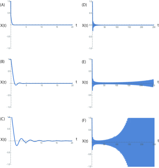
Figure 1: Dynamics of Equation (13) via Numerical Simulation: The parameters are set as $a=1.0,b=-2.0$, with a constant initial interval function $X(t)=1.0$, $(-\tau\leq t\leq 0)$. The values of the delays $\tau$ are (A)$0.2$, (B)$0.5$, (C)$0.7$, (D)$0.75$, (E)$0.8$, (F)$0.82$.

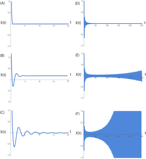
Figure 2: Approximation of the Dynamics of Equation (13) by Equation (15): The parameters remain consistent with those in Figure 1, where $a=1.0$, $b=-2.0$, and the constant initial interval function is $X(t)=1.0$ for $(-\tau\leq t\leq 0)$. The delays $\tau$ take values (A)$0.2$, (B)$0.5$, (C)$0.7$, (D)$0.75$, (E)$0.8$, (F)$0.82$.

4 Analysis of reviving dynamics

In the approximate solution (15) , the amplitude of oscillation is determined by the function:

$$f(t)=X_{0}({1\over t})^{a}Re[e^{{1\over\tau}W_{0}(b\tau)t}]=X_{0}({1\over t})^{a}e^{{1\over\tau}Re[W_{0}(b\tau)]t}.$$ (16)

To observe the change in this amplitude, we calculate its derivative:

$${df(t)\over dt}=-X_{0}({1\over t})^{a+1}(a-({t\over\tau}Re[W_{0}(b\tau)])e^{{1\over\tau}Re[W_{0}(b\tau)]t}.$$ (17)

Here, we assume $X_{0}>0$, $\tau\geq 0$ and consider $t>0$ as in the parameters in Figure 1. Then

$${df(t)\over dt}<0\iff Re[W_{0}(b\tau)]<{{a\tau}\over t}.$$ (18)

and

$${df(t)\over dt}=0\iff Re[W_{0}(b\tau)]={{a\tau}\over t}.$$ (19)

These lead to the following results:

$${df(t)\over dt}<0,\quad\forall t>0\iff Re[W_{0}(b\tau)]<0.$$ (20)

The time $t_{min}$ that minimizes the amplitude is determined by

$${df\over dt}(t_{min})=0.$$ (21)

Hence,

$$t_{min}={a\tau\over Re[W_{0}(b\tau)]}.$$ (22)

In Figure 3, we have plotted $Re[W_{0}(b\tau)]$ and $t_{min}$ as functions of $\tau$. It is also known from the property of the $W$ function that if $\tau_{c}=-{\pi\over{2b}}$, then $Re[W_{0}(b\tau_{c})]=0$.

From these observations, we can infer the following:

• For $0<\tau<\tau_{c}$, the origin is a stable fixed point, and the amplitude of oscillation monotonically decreases.

• At $\tau\geq\tau_{c}$, the stability of the origin is lost, and the dynamics diverge. However, reviving dynamics with minimum amplitude $X_{min}$ occur approximately at $t_{min}$

• There exists the smallest $t_{min}$ as a function of the delay $\tau$. In other words, tuning the value of the delay $\tau$ allows for the shortest reviving switching point.

• We note that with this parameter set, the value of the $t_{min}$ can be less than $\tau$ (Fig. 3). The choice of the initial function can influence the dynamics near this smallest $t_{min}$. However, within the range of $t_{min}>\tau$, our approximation works effectively, as depicted in Fig. 4 (A), (B), (C).

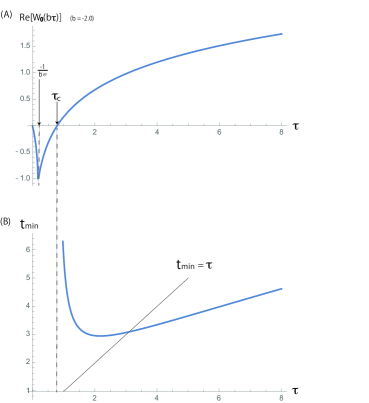
Figure 3: The plots depict (A) the real part of $W_{0}$ function with $b=-2.0$, and (B) the time, $t_{min}$, t which the amplitude is at its minimum. The reviving dynamics occur for $\tau>\tau_{c}=-{\pi\over{2b}}\approx 0.785$. The smallest value of $t_{min}$ is estimated to be $2.935$ when $\tau\approx 2.182$. Also, $\tau=\tau_{min}\approx 3.074$.

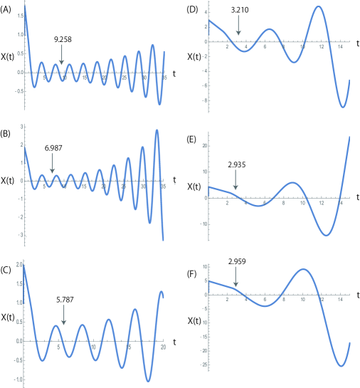
Figure 4: Dynamics of the Model via Numerical Simulation for $t_{min}>\tau$: The arrows indicate the values of $t_{min}$, representing the reviving time point where the amplitude is at its minimum, as estimated by the approximation (22). The delays $\tau$ take the values (A)$0.9$, (B)$0.95$, (C)$1.0$, (D)$1.5$, (E)$2.18$, (F)$2.5$.

5 Discussion

This paper delves into the unexplored realm of reviving dynamics in delay differential equations. Through a combination of numerical computations and the application of approximate expressions employing the $W$ function, we have successfully unveiled the characteristics of this phenomenon. While previous research has delved into the concept of specific delay values inducing resonance in systems with delay feedback [26, 20, 21], the phenomenon explored in this paper also exhibits common traits, including the emergence of a minimum value for the reviving time point.

Our aspiration is that within the class of delay differential equations, where approximate solutions using the $W$ function are derived in this paper, various transient phenomena can be further analyzed. This analytical exploration represents another avenue towards achieving a broader understanding of the intricate dynamics within delay systems.

References

- [1] U. an der Heiden. Delays in physiological systems. J. Math. Biol., 8:345–364, 1979.
- [2] R. Bellman and K. Cooke. Differential-Difference Equations. Academic Press, New York, 1963.
- [3] J. L. Cabrera and J. G. Milton. On–off intermittency in a human balancing task. Phys. Rev. Lett., 89:158702, 2002.
- [4] N. D. Hayes. Roots of the transcendental equation associated with a certain difference–differential equation. J. Lond. Math. Soc., 25:226–232, 1950.
- [5] T. Insperger. Act-and-wait concept for continuous-time control systems with feedback delay. IEEE Trans. Control Sys. Technol., 14:974–977, 2007.
- [6] U. Küchler and B. Mensch. Langevin’s stochastic differential equation extended by a time-delayed term. Stoch. Stoch. Rep., 40:23–42, 1992.
- [7] A. Longtin and J. G. Milton. Insight into the transfer function, gain and oscillation onset for the pupil light reflex using delay-differential equations. Biol. Cybern., 61:51–58, 1989.
- [8] M. C. Mackey and L. Glass. Oscillation and chaos in physiological control systems. Science, 197:287–289, 1977.
- [9] L. Glass, A. Beuter, and D. Larocque. Time delays, oscillations, and chaos in pysiological control systems. Mathematical Biosciences, 90:111–125, 1988.
- [10] L. Glass and M. C. Mackey. From Clocks to Chaos: The rhythms of life. Princeton University Press, Princeton, New Jersey, 1988.
- [11] J Mitlon, J. L. Cabrera, T. Ohira, S. Tajima, Y. Tonosaki, C. W. Eurich, and S. A. Campbell. The time–delayed inverted pendulum: Implications for human balance control. Chaos, 19:026110, 2009.
- [12] T. Ohira and T. Yamane. Delayed stochastic systems. Phys. Rev. E, 61:1247–1257, 2000.
- [13] H. Smith. An introduction to delay differential equations with applications to the life sciences. Springer, New York, 2010.
- [14] G. Stépán. Retarded dynamical systems: Stability and characteristic functions. Wiley & Sons, New York, 1989.
- [15] G. Stépán and T. Insperger. Stability of time-periodic and delayed systems: a route to act-and-wait control. Ann. Rev. Control, 30:159–168, 2006.
- [16] M. Szydlowski and A. Krawiec. The Kaldor–Kalecki model of business cycle as a two-dimensional dynamical system. J. Nonlinear Math. Phys., 8: 266–271, 2010.
- [17] S. R.Taylor and S. A. Campbell. Approximating chaotic saddles for delay differential equations. Phys. Rev. E, 75: 046215, 2007.
- [18] J. Milton, P. Naik, C. Chan, and S. A. Campbell. Indecision in neural decision making models. Math. Model. Nat. Phenom., 5:125–145, 2010.
- [19] K. Pakdaman, C. Grotta-Ragazzo, and C. P. Malta. Transient regime duration in continuous-time neural networks with delay. Phys. Rev. E, 58:3623–3627, 1998.
- [20] K. Ohira. Resonating Delay Equation. EPL, 137: 23001, 2022.
- [21] K. Ohira and T. Ohira. Delayed Dynamics with Transient Resonating Oscillations. J. Phys. Soc. Japan, 92: 064002, 2023. (ArXiv: 2201.12058 includes corrections.)
- [22] K. Ohira and T. Ohira. Delay, resonance and the Lambert W function. ArXive: 2301.13448, 2023.
- [23] R. M. Corless, G. H. Gonnet, D. E. G. Hare, D. J. Jeffrey, D. E. Knuth. On the Lambert W function Advances in Computational Mathematics, 5: 329–359, 1996.
- [24] H. Shinozaki and T. Mori. Robust stability analysis of linear time delay system by Lambert W function. Automatica, 42: 1791–1799, 2006.
- [25] R. Pusenjak. Application of Lambert function in the control of production systems with delay. Int. J. Eng. Sci, 6: 28–38, 2017.
- [26] T. Ohira and Y. Sato. Resonance with noise and delay. Phys. Rev. Lett., 82:2811–2815, 1999.