Pulsar Timing Arrays and
Primordial Black Holes from a Supercool Phase Transition

Abstract

An explicit realistic model featuring a supercool phase transition, which allows us to explain the background of gravitational waves recently detected by pulsar timing arrays, is constructed. In this model the phase transition corresponds to radiative symmetry breaking (and mass generation) in a dark sector featuring a dark photon associated with the broken symmetry. The completion of the transition is ensured by a non-minimal coupling between gravity and the order parameter and fast reheating occurs thanks to a preheating phase. Finally, it is also shown that the model leads to primordial black hole production.

1 Introduction

Gravitational wave (GW) astronomy has become an extremely active and exciting field of physics after the discovery of GWs from binary black-hole and neutron-star mergers [1, 2, 3]. More recently, the interest in this field has been further increased by the detection of a background of GWs by pulsar timing arrays (PTAs), including the North American Nanohertz Observatory for Gravitational Waves (NANOGrav), the Chinese Pulsar Timing Array (CPTA), the European Pulsar Timing Array (EPTA) and the Parkes Pulsar Timing Array (PPTA) [4, 5, 6, 7].

Among several possibilities to interpret the PTA background, an interesting option is first-order phase transitions (PTs). Indeed, these phenomena are not present in the Standard Model (SM) and, therefore, the detection of a GW background generated in this way (see Ref. [8] for a textbook introduction) would be clear evidence for new physics. A PT interpretation of the signals detected by PTAs performed by the NANOgrav collaboration and relevant for the present study was provided in Ref. [9] and other independent discussions of PT interpretations were given e.g. in Refs. [10, 11, 12, 13, 14, 15, 16, 17, 18, 19, 20, 21, 22, 23, 24, 25, 26, 27, 28, 29, 30, 31].

First-order PTs generally occur when the symmetries are predominantly broken (and masses are then generated) through radiative corrections [32, 33, 34, 35] (see Ref. [36] for a review). This radiative symmetry breaking (RSB) is interesting also because it has the unique property of allowing a perturbative (and thus calculable) description of PTs [35]. Another distinctive property of such PTs is the presence of a period of supercooling when the temperature dropped much below the critical temperature [34, 35].

The GW background detected by PTAs could be due to a supercool PT associated with an RSB at a scale around the GeV [27, 28]. However, so far a concrete model with these characteristics has not been found and, therefore, its existence has not been guaranteed. Indeed, as pointed out in [19], identifying such a model is very challenging.

As a proof of concept, the purpose of this paper is to solve this issue by constructing an explicit realistic model that can explain the PTA background through a supercool PT associated with RSB.

Besides generating a GW background, supercool PT associated with an RSB also naturally lead to primordial black hole (PBH) production through the “late-blooming mechanism” (see e.g. Refs. [37, 38, 39, 40, 41] for a quantitative introduction): since the false vacuum decay of PTs is statistical for quantum and thermal reasons, in distinct patches the transition can occur at different times. Patches where the transition occurs the latest undergo the longest vacuum-dominated stage and, therefore, develop large over-densities, which collapse into PBHs. These PBHs can then account for a fraction $f_{\rm{PBH}}$ of the dark matter density.

Another purpose of the present work is to identify regions of the parameter space of the above-mentioned model where the PBH production is significant and the PTA detection is explained at the same time. In the following sections we show that all this is possible and in the last section we highlight the main results achieved.

2 A minimal model

Let us start by considering a classically scale-invariant dark sector with RSB at the GeV scale. The simplest option is the Coleman-Weinberg construction [32], which features an Abelian gauge symmetry, $U(1)_{D}$, and a charged scalar field $\phi$. The corresponding no-scale Lagrangian is given by

$$\mathscr{L}^{\rm ns}=-\frac{1}{4}\mathcal{A}_{\mu\nu}\mathcal{A}^{\mu\nu}+(D_{\mu}\phi)^{\dagger}\,D^{\mu}\phi-\frac{1}{4}\lambda_{\chi}\chi^{4},$$ (1)

where $\mathcal{A}_{\mu\nu}\equiv\partial_{\mu}\mathcal{A}_{\nu}-\partial_{\nu}\mathcal{A}_{\mu}$ (the vector $\mathcal{A}_{\mu}$ is the $U(1)_{D}$ gauge boson), $\chi\equiv\sqrt{2}|\phi|$ and $D_{\mu}\phi=(\partial_{\mu}+ie_{d}\mathcal{A}_{\mu})\phi$ (the parameter $e_{d}$ is the $U(1)_{D}$ gauge coupling). The symmetry $U(1)_{D}$ is the one that undergoes RSB. This happens through a radiatively induced VEV of $\chi$ at the required energy scale, $\chi_{0}\sim\leavevmode\nobreak\$GeV. As well known, RSB takes place because quantum corrections produce the following one-loop effective potential for $\chi$

$$V_{q}(\chi)=\frac{\bar{\beta}}{4}\left(\log\frac{\chi}{\chi_{0}}-\frac{1}{4}\right)\chi^{4},$$ (2)

where

$$\bar{\beta}\equiv\left[\mu\frac{d\lambda_{\chi}}{d\mu}\right]_{\mu=\tilde{\mu}}>0$$ (3)

and $\tilde{\mu}$ is a value of the renormalization group scale $\mu$ at which $\lambda_{\chi}=0$.

However, the dark sector here interacts with the SM. Besides gravity, which is very weak, there are two possible operators that can mediate such interactions. One is the Higgs portal

$$\mathscr{L}_{\chi h}=\frac{1}{2}\lambda_{\chi h}\chi^{2}|{\mathcal{H}}|^{2},$$ (4)

where ${\mathcal{H}}$ is the SM Higgs doublet and $\lambda_{\chi h}$ is the corresponding quartic coupling. The other one is a kinetic mixing between the SM photon, $\mathcal{F}_{\mu}$, and $\mathcal{A}_{\mu}$:

$$\mathscr{L}_{\rm mix}=-\frac{\eta}{2}\mathcal{A}_{\mu\nu}\mathcal{F}^{\mu\nu},$$ (5)

where $\mathcal{F}_{\mu\nu}\equiv\partial_{\mu}\mathcal{F}_{\nu}-\partial_{\nu}\mathcal{F}_{\mu}$ and $\eta$ is the mixing parameter.

In general we can also introduce a non-minimal coupling $\xi_{\chi}$ appearing in the Lagrangian density through the term

$$-\frac{1}{2}\xi_{\chi}\chi^{2}R,$$ (6)

where $R$ is the Ricci scalar. The pure-gravity Lagrangian is assumed to be the standard Einstein-Hilbert one at the energies that are relevant for this work. Note that the term in (6) does not lead to an appreciable modification of gravity in our case because $\chi_{0}\sim\leavevmode\nobreak\$GeV$\leavevmode\nobreak\ \ll M_{P}$, unless one takes $\xi_{\chi}$ extremely large, which we do not. However, as will be shown in Sec. 3, that term can ensure that the PT completes.

The mixing in (5) can be removed by performing the field redefinition $\{\mathcal{A}_{\mu},\mathcal{F}_{\mu}\}\to\{A^{\prime}_{\mu},A_{\mu}\}$ given by

$$\left(\begin{array}[]{c}\mathcal{A}_{\mu}\\ \mathcal{F}_{\mu}\\ \end{array}\right)=\left(\begin{array}[]{cc}\frac{1}{\sqrt{1-\eta^{2}}}&0\\ -\frac{\eta}{\sqrt{1-\eta^{2}}}&1\\ \end{array}\right)\left(\begin{array}[]{c}A^{\prime}_{\mu}\\ A_{\mu}\\ \end{array}\right).$$ (7)

However, after this field redefinition, $\eta$ still appears in the Lagrangian because

$$(D_{\mu}\phi)^{\dagger}\,D^{\mu}\phi=(\partial_{\mu}\phi)^{\dagger}\,\partial^{\mu}\phi+\frac{e_{d}^{2}\chi^{2}A^{\prime}_{\mu}A^{\prime\mu}}{2(1-\eta^{2})}+\frac{e_{d}J^{\prime}_{\mu}A^{\prime\mu}}{\sqrt{1-\eta^{2}}},$$ (8)

with $J^{\prime}_{\mu}\equiv i\left[\left(\partial_{\mu}\phi\right)^{\dagger}\phi-\phi^{\dagger}\partial_{\mu}\phi\right]$, and because of the interaction term $eJ_{\mu}\mathcal{F}^{\mu}$ between $\mathcal{F}_{\mu}$ and the SM electromagnetic current $J_{\mu}$, i.e.

$$eJ_{\mu}\mathcal{F}^{\mu}=eJ_{\mu}A^{\mu}-\frac{e\eta J_{\mu}A^{\prime\mu}}{\sqrt{1-\eta^{2}}}.$$ (9)

The second term in the right-hand side of (8) leads to a background-dependent squared mass of the “dark photon” $A^{\prime}_{\mu}$, namely $m_{d}^{2}(\chi)=e_{d}^{2}\chi^{2}/(1-\eta^{2}).$ After RSB $\chi$ acquires a VEV $\chi_{0}$ and this leads to the dark photon mass $m_{d}(\chi_{0})$. Since in our current setup $\chi_{0}$ is much smaller than the EW scale and we demand the validity of perturbation theory ($e_{d}$ must not be large), $m_{d}(\chi_{0})$ should be much smaller than the EW scale too.

The second term in the right-hand side of (9) is instead an interaction between $J_{\mu}$ and $A^{\prime}_{\mu}$. Therefore, in order to satisfy the experimental limits $\eta$ should be small (see [42, 43] for reviews). So

$$m_{d}^{2}(\chi)\approx e_{d}^{2}\chi^{2},\leavevmode\nobreak\ \leavevmode\nobreak\ \frac{J^{\prime}_{\mu}A^{\prime\mu}}{\sqrt{1-\eta^{2}}}\approx J^{\prime}_{\mu}A^{\prime\mu},\leavevmode\nobreak\ \leavevmode\nobreak\ \frac{\eta J_{\mu}A^{\prime\mu}}{\sqrt{1-\eta^{2}}}\approx\eta J_{\mu}A^{\prime\mu}$$ (10)

and the dark photon is coupled to the electromagnetic current through a millicharge $e\eta$. The Higgs portal coupling $\lambda_{\chi h}$ should also be very small because the mass $m_{\chi}$ of $\delta\chi\equiv\chi-\chi_{0}$ is also much smaller than the EW scale: $m_{\chi}=\sqrt{\beta_{\chi}}\chi_{0}\ll\chi_{0}\sim\leavevmode\nobreak\$GeV. Note that the smallness of $\lambda_{\chi h}$ and $\eta$ (and of gravity) ensures that, barring quantum corrections, the scale invariance of the dark sector is only mildly broken by its interactions.

3 The (improved) supercool expansion

As recalled in the introduction, in a PT associated with RSB supercooling always occur. The field $\chi$ is trapped in the false minimum, $\chi=0$, for a long time during which the space expands exponentially with Hubble rate

$$H_{I}=\frac{\sqrt{\bar{\beta}}\chi_{0}^{2}}{4\sqrt{3}M_{P}},$$ (11)

where $M_{P}$ is the reduced Planck mass. After that $\chi$ goes towards the true minimum, $\chi_{0}$, and reheating occurs up to a temperature $T_{r}$ at most given by

$$T_{r}^{4}\approx\frac{15\bar{\beta}\chi_{0}^{4}}{8\pi^{2}g_{*}(T_{r})},$$ (12)

where $g_{*}(T)$ is the effective number of relativistic species at temperature $T$.

The amount of supercooling that actually takes place depends on the model and can be parameterized by [35]

$$\epsilon\equiv\frac{g^{4}}{6\bar{\beta}\log\frac{\chi_{0}}{T}},$$ (13)

where $g$ plays the role of a “collective coupling” of $\chi$ with all fields of the theory: in the model of Sec. 2,

$$g=\sqrt{3}|e_{d}|,\qquad\bar{\beta}=\frac{6e_{d}^{4}}{(4\pi)^{2}}=\frac{2g^{4}}{3(4\pi)^{2}}.$$ (14)

The larger the supercooling, $T\ll\chi_{0}$, the smaller $\epsilon$.

As shown in [35] and [28], if $\epsilon\ll 1$, one can describe the PT, as well as the GW spectrum and the PBH production, with good accuracy by means of a small-$\epsilon$ expansion (called “supercool expansion”). If $T_{r}$ is given by (12), at leading order (LO) one can parameterize the relevant physics in terms of $\chi_{0}$, $g$, $\bar{\beta}$ and $g_{*}$ only, while at next-to-leading order (NLO) one must introduce an extra parameter $\tilde{g}$, which in the model of Sec. 2 is $\tilde{g}=g/\sqrt[6]{3}$. At LO the nucleation temperature $T_{n}$ (defined as the temperature at which the false-vacuum decay rate per unit volume $\Gamma_{v}$ equals $H_{I}^{4}$), can be computed with the simple formula

$$T_{n}\approx\chi_{0}\exp\left(\frac{\sqrt{c^{2}-16a}-c}{8}\right),$$ (15)

with

$$a\equiv\frac{c_{3}g}{\sqrt{12}\bar{\beta}},\quad c_{3}=18.8973...\quad c\equiv 4\log\frac{4\sqrt{3}M_{P}}{\sqrt{\bar{\beta}}\,\chi_{0}}+\frac{3}{2}\log\frac{a}{2\pi}.$$

If one wants to describe not only models with $\epsilon\ll 1$, but also those with $\epsilon$ of order 1, one can again describe the relevant physics perturbatively in the amount of supercooling, but through an improved version of the supercool expansion [28], where one has to exactly take $\tilde{g}$ into account at any order [28]. In this “improved supercool expansion” $T_{n}$ can be computed with a more complex procedure explained in [28].

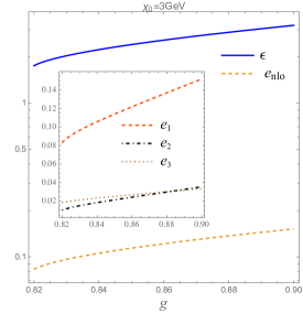
Figure 1: Comparison between $\epsilon$ and the error $e_{nlo}$ that one is making in using the standard supercool expansion at NLO in the minimal model of Sec. 2. The inset shows the three sources of errors defined in (16). Varying $\chi_{0}$ around the GeV scale does not show significant differences: a plot corresponding to another value of $\chi_{0}$ is shown in the appendix.

Let us now quantify the error that one is making in analysing the model of Sec. 2 with the standard supercool expansion at NLO. Fig. 1 shows $\epsilon$ as well as $e_{nlo}\equiv\max(e_{1},e_{2},e_{3})$ and $(e_{1},e_{2},e_{3})$ defined by

$$(e_{1},e_{2},e_{3})\equiv\left(\frac{\tilde{c}_{3}^{2}\tilde{g}^{6}\epsilon}{2\pi^{2}c_{3}^{2}g^{6}},\frac{|\frac{1}{2}\log(\epsilon/g^{2})-1/4|}{\log\frac{\chi_{0}}{T_{n}}},\frac{\epsilon}{96}\right)$$ (16)

(computed for simplicity with the LO formula for $T_{n}$ in (15)) with $\tilde{c}_{3}=31.6915...$ . As discussed in [28], $e_{1}$ quantifies the above-mentioned error, while $e_{2}$ and $e_{3}$ are estimates of the errors present also in the improved supercool expansion at leading order. Fig. 1 tells us that such improved supercool expansion is valid and a better approximation than the standard supercool expansion as $\epsilon\sim 1$ and $\{e_{1}>e_{2},e_{1}>e_{3}\}$ in this model. Therefore, in the rest of the paper we will use the improved supercool expansion.

In general the existence of $T_{n}$ restricts the parameter space [28]. One might wonder if the PT always complete, especially in the region of the parameter space where $T_{n}$ does not exist. If $\Gamma_{v}$ is not large enough to ensure the completion of the PT the temperature keeps decreasing and eventually the effect of the spacetime curvature, as well as quantum fluctuations, can become important in the decay rate [44, 45, 46, 47]. This can lead to the completion of the transition. Indeed, during the exponential expansion, the non-minimal coupling in (6), with $\xi_{\chi}$ positive, gives a tachyonic mass contribution, $-6\xi_{\chi}H_{I}^{2}\chi^{2}$, to the effective potential of $\chi$, which makes the transition complete when, eventually, the spacetime curvature dominates over thermal fluctuations.

4 Preheating and reheating

Can one has a sufficiently high reheating temperature $T_{r}$ in this model through direct decays of $\chi$ into SM particles? The answer to this question seems negative for the following reason.

The only tree-level channels for the decay of $\delta\chi$ into SM particles are $\chi\to A^{\prime}A^{\prime}(HH)\to$ 4 fermions, where the intermediate $A^{\prime}$s and Higgs bosons $H$ are virtual because an on-shell $A^{\prime}$ or $H$ is much heavier than $\delta\chi$ in our setup. The decays of $A^{\prime}$ and $H$ into fermions are allowed by the interaction with the electromagnetic current in (10) and the Yukawa couplings, respectively. Dropping the external legs, the amplitudes for these processes for light-enough leptons are of order $e_{d}^{2}\chi_{0}(e\eta)^{2}/m_{d}^{4}(\chi_{0})$ and $\lambda_{\chi h}\chi_{0}y_{\rm SM}^{2}/M_{h}^{4}$, respectively, where the denominators $m_{d}^{4}(\chi_{0})$ and $M_{h}^{4}$ are due to the low energy limit of the two $A^{\prime}$ or $H$ propagators and $y_{\rm SM}$ is the SM Yukawa coupling of a light SM fermion. Taking the absolute value squared of the amplitude and integrating over the four-body phase space to obtain the decay rate $\Gamma$ one finds

$$\Gamma(\chi\to A^{\prime}A^{\prime}\to 4\leavevmode\nobreak\ \mbox{leptons})\lesssim m_{\chi}^{7}\left(\frac{e_{d}^{2}\chi_{0}(e\eta)^{2}}{m_{d}^{4}(\chi_{0})}\right)^{2},$$ (17)

$$\Gamma(\chi\to HH\to 4\leavevmode\nobreak\ \mbox{leptons})\lesssim m_{\chi}^{7}\left(\frac{\lambda_{\chi h}\chi_{0}y_{\rm SM}^{2}}{M_{h}^{4}}\right)^{2}$$ (18)

or even smaller because of four-body phase-space suppressions. The factor $m_{\chi}^{7}$ has been inserted for dimensional reasons. Setting $\eta$ compatible with the experimental limits, $\chi_{0}\lesssim 10$ GeV and $g$ to realistic values compatible with the PTA GW signal, one finds that these channels can reheat the universe only up to a reheating temperature below the MeV scale, too small to realize a sufficiently fast reheating, where $T_{r}$ is rather given by the last equation in (12).

Let us then consider the preheating phase [48, 49, 50, 51], when production of particles interacting with $\chi$ occurs as a result of the time dependence of this field through parametric resonance. In this model the only particle with a sizable coupling with $\chi$ is $A^{\prime}$ and its field equations are

$$\frac{1}{\sqrt{|\det\hat{g}|}}\partial_{\nu}\left(\sqrt{|\det\hat{g}|}\,F^{\prime\mu\nu}\right)=m_{d}^{2}(\chi)A^{\prime\mu}+e_{d}J^{\prime\mu}-e\eta J^{\mu},$$ (19)

where $\det\hat{g}$ is the determinant of the spacetime metric, $F^{\prime}_{\mu\nu}\equiv\partial_{\mu}A^{\prime}_{\nu}-\partial_{\nu}A^{\prime}_{\mu}$ and we have used the smallness of $\eta$. After the false vacuum decay has taken place mostly of the energy stored in $\chi$ is thus transferred to $A^{\prime}$ because $H_{I}^{4}$ is tiny compared to the potential density in the setup under study.

At some stage $\chi$ undergoes small oscillations around $\chi_{0}$. In such a regime one can analytically show that most of the energy density stored in $\chi$ is efficiently transferred to $A^{\prime}$ as we now do. In that case, the dependence of $\chi$ on the cosmic time $t$ is given by

$$\chi(t)=\chi_{0}+\Phi\sin(m_{\chi}t),$$ (20)

with $\Phi\ll\chi_{0}$, and the background dependent mass $m_{d}(\chi)\sim e_{d}\chi_{0}$ is generically extremely large compared to $H_{I}$ (see Eq. (11)). So we can neglect the expansion of the universe. Recalling that $\eta$ must be very small and setting the unitary gauge, where $J^{\prime}_{\mu}=0$, Eq. (19) then reads

$$\partial_{\nu}\,F^{\prime\mu\nu}=m_{d}^{2}(\chi)A^{\prime\mu}.$$ (21)

Taking the divergence of this equation and inserting the result back into Eq. (21) gives

$$-\partial_{\nu}\partial^{\nu}A^{\prime}_{\mu}=m_{d}^{2}(\chi)A^{\prime}_{\mu}+\partial_{\mu}\left(\frac{A^{\prime\nu}\partial_{\nu}m_{d}^{2}(\chi)}{m_{d}^{2}(\chi)}\right).$$ (22)

In the regime (20) with $\Phi\ll\chi_{0}$ the second term in the right-hand side of the equation above is negligible with respect to the first one because suppressed by extra powers of $\chi_{0}$ in the denominator and of $m_{\chi}=\sqrt{\bar{\beta}}\chi_{0}\ll\chi_{0}$ in the numerator:

$$\begin{array}[]{c}\left\{\begin{array}[]{c}m_{d}^{2}(\chi)A^{\prime}_{\mu}\approx e_{d}^{2}(\chi_{0}^{2}+2\chi_{0}\Phi\sin(m_{\chi}t))A^{\prime}_{\mu}\\ \partial_{\mu}\left(\frac{A^{\prime\nu}\partial_{\nu}m_{d}^{2}(\chi)}{m_{d}^{2}(\chi)}\right)\approx\partial_{\mu}\left(\frac{A^{\prime}_{0}2\chi_{0}\Phi m_{\chi}\cos(m_{\chi}t)}{\chi_{0}^{2}}\right)\end{array}\right..\end{array}$$ (23)

So the field equations of $A^{\prime}$ simply reduce to that of a scalar with a quartic portal interaction with $\chi^{2}$. Working in the Fourier space of momenta $\vec{k}$, all three polarizations $A^{\prime}_{k}$ of the dark photons are then well described by the equation

$$\ddot{A}^{\prime}_{k}+(k^{2}+e_{d}^{2}\chi_{0}^{2}+2e_{d}^{2}\chi_{0}\Phi\sin(m_{\chi}t))A^{\prime}_{k}=0,$$ (24)

with $k\equiv|\vec{k}|$. This equation can now be brought into the well-known Mathieu equation:

$$\frac{d^{2}A_{k}^{\prime}}{dz^{2}}+(a_{k}-2q\cos(2z))A^{\prime}_{k}=0,$$ (25)

where $a_{k}\equiv 4(k^{2}+e_{d}^{2}\chi_{0}^{2})/m_{\chi}^{2}$, $q\equiv 4e_{d}^{2}\chi_{0}\Phi/m_{\chi}^{2}$ and $z\equiv m_{\chi}t/2+\pi/4$. Therefore, as explained in [52, 51], there is an exponential growth of the dark photon field, $A_{k}^{\prime}\sim\exp(\mu_{k}^{(n)}z)$, which corresponds to an equally explosive growth of dark photon occupation numbers of quantum fluctuations when $k$ belongs to some resonance bands labelled by an arbitrary integer $n$. These ranges of values of $k$ always exist and the constants of the exponential growth, the $\mu_{k}^{(n)}$, allow to efficiently transfer all the energy density stored in the inflaton to the dark photon in a negligible cosmic time. This exponential growth cannot last forever because of the backreaction of $A^{\prime}$ on $\chi$: when $A^{\prime}$ grows $\chi$ feels a growing effective mass, which makes $\chi$ tend to a vanishing value as time passes.

However, the preheating phase allows to transfer the vacuum energy density $\rho_{V}$ to $A^{\prime}$, which can then decay into pairs of SM fermions, thanks to the interaction with $J_{\mu}$ in (10). The corresponding tree-level decay rate into lepton pairs is

$$\Gamma(A^{\prime}\to 2\leavevmode\nobreak\ \mbox{leptons})=\frac{(\eta e)^{2}m_{d}(\chi_{0})}{12\pi}\Phi_{s}(m_{d}(\chi_{0}),m_{l}),$$ (26)

where $m_{l}$ is the lepton mass and the phase space factor $\Phi_{s}$ is

$$\Phi_{s}(m_{d},m_{l})=\sqrt{1-\left(\frac{2m_{l}}{m_{d}}\right)^{2}}\left(1+\frac{2m_{l}^{2}}{m_{d}^{2}}\right)\theta(m_{d}-2m_{l}).$$ (27)

Unlike for the decays of $\delta\chi$ into four SM fermions, which we have previously discussed, setting $\eta$ compatible with the experimental limits, $\chi_{0}\lesssim 10$ GeV and $g$ compatible with the PTA GW signal and all observational constraints, one finds that these processes allows for a very fast reheating. Including the hadronic decay channel of $A^{\prime}$ reinforces this result. Because $\rho_{V}$ represents the full energy budget of the system, the value of $T_{r}$ given by the last equation in (12) is the correct value of the reheating temperature in this model.

5 Gravitational waves and primordial black holes

In the improved supercool expansion one can also obtain accurate expressions for $\beta/H_{n}$, where $\beta$ is the inverse duration of the PT and $H_{n}$ is the Hubble rate at $T=T_{n}$, as well as the GW spectrum and its red-shifted frequency peak today $f_{\rm peak}$ [28]. Moreover, it can be used to describe the PBH late-blooming mechanism in terms of the few parameters $\chi_{0}$, $g$, $\bar{\beta}$ and $\tilde{g}$ [28]. We now make use of these results in the context of the minimal model of Sec. 2.

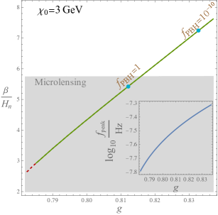
Figure 2: $\beta/H_{n}$, and (in the inset) $f_{\rm peak}$ in the minimal model of Sec. 2 and computed with the improved supercool expansion. Here $g_{*}(T_{r})=6$, although the plot depends weakly on $g_{*}$. Values of $g$ corresponding to the green solid line reproduce the NANOGrav signal at 68% C.L.; all displayed values of $g$ correspond to $\epsilon$ at most of order 1, so the improved supercool expansion can be trusted. The shaded region is constrained by microlensing.

Fig. 2 shows the predictions of this model for $\beta/H_{n}$ and $f_{\rm peak}$ setting $\chi_{0}$ at the GeV scale. The plot shows that there are values of $g$ such that this model reproduces the GW background detected by PTAs and is not excluded by other observations. In particular the values of $g$ corresponding to $f_{\rm PBH}=1$ and $f_{\rm PBH}=10^{-10}$ and the microlensing constraints [53, 54, 55, 56] (the strongest constraints on PBHs in the setup of Fig. 2) are given. These PBHs weight about a solar mass [27].

In the appendix we provide the corresponding plots for other values of $\chi_{0}$ around the GeV scale. These have the same qualitative feature. Also, as expected, they show that when $\chi_{0}$ goes above the GeV scale the values of $g$ that can reproduce the PTA GW background tend to disappear.

Furthermore, although PBHs are produced, one cannot account for the entire dark matter abundance through PBHs, as clear in Fig. 2. One can complete the dark matter abundance as well as reproduce the observed neutrino oscillations and matter antimatter asymmetry by introducing, for example, three right-handed neutrinos along the lines of Refs. [57, 58, 59, 60, 61, 62, 63]. Since neutrinos are not charged under $U(1)_{D}$ and do not appear in the electromagnetic current, the preheating and reheating analysis of Sec. 4 remains valid.

6 Conclusions

We have constructed and studied an explicit realistic model featuring RSB (and thus an associated supercool PT) that explains the background of GWs found by PTAs. The model features a simple dark sector, which involves the field $\chi$ responsible for RSB and a hidden photon that can interact with the SM particles through a mixing with the SM photon. The completion of the transition is ensured by a non-minimal coupling between $\chi$ and $R$. Moreover, fast reheating after the supercool PT occurs thanks to a preheating phase, where the vacuum energy density stored in $\chi$ is transferred to the dark photon, which can then decay to SM fermions via the mixing. Finally, we have also identified regions of the parameter space where one has significant PBH production.

The work presented here opens several research directions. As an outlook example, it would be interesting to generalize the dark sector: the model presented here is the minimal RSB one able to reproduce the GW background detected by PTAs, but one can introduce other scalar, vector and fermion fields with sizable couplings to $\chi$. Moreover, it would be valuable to extend the preheating analysis reported here to a general PT associated with RSB in order to identify in a model-independent way the parameter space corresponding to fast reheating. Finally, the interaction between the theoretical and observational community (PTAs, the LIGO and VIRGO collaborations for GW detection, etc.) will be vital to further probe this scenario.

Appendix A
Varying the symmetry breaking scale

In this appendix the plots in Figs. 1 and 2 are extended to other values of $\chi_{0}$ . This is done to illustrate the quantitative dependence on the symmetry breaking scale $\chi_{0}$.

Fig. 3 shows that varying $\chi_{0}$ around the GeV scale does not significantly change the plot in Fig. 1.

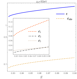
Figure 3: Like in Fig. 1, but with $\chi_{0}=5GeV$.

Fig. 4 shows that varying $\chi_{0}$ around the GeV scale in Fig. 2 leads to qualitatively similar plots, apart from the expected fact that when $\chi_{0}$ goes above the GeV scale, the values of $g$ that can reproduce the PTA GW background tend to disappear.

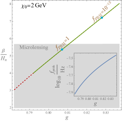
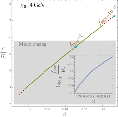
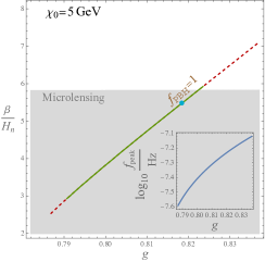
Figure 4: Like in Fig. 2, but for other values of $\chi_{0}$ around the GeV scale.

References

References

- [1] B. P. Abbott et al. [LIGO Scientific and Virgo Collaborations], “Observation of Gravitational Waves from a Binary Black Hole Merger,” Phys. Rev. Lett. 116, 061102 (2016) doi:10.1103/PhysRevLett.116.061102 [arXiv:1602.03837].
- [2] B. Abbott et al. [LIGO Scientific and Virgo], “GW150914: Implications for the stochastic gravitational wave background from binary black holes,” Phys. Rev. Lett. 116, no.13, 131102 (2016) doi:10.1103/PhysRevLett.116.131102 [arXiv:1602.03847].
- [3] B. P. Abbott et al. “Multi-messenger Observations of a Binary Neutron Star Merger,” Astrophys. J. Lett. 848 (2017) no.2, L12 doi:10.3847/2041-8213/aa91c9 [arXiv:1710.05833].
- [4] G. Agazie et al. [NANOGrav], “The NANOGrav 15 yr Data Set: Evidence for a Gravitational-wave Background,” Astrophys. J. Lett. 951 (2023) no.1, L8 doi:10.3847/2041-8213/acdac6 [arXiv:2306.16213].
- [5] J. Antoniadis, P. Arumugam, S. Arumugam, S. Babak, M. Bagchi, A. S. B. Nielsen, C. G. Bassa, A. Bathula, A. Berthereau and M. Bonetti, et al. “The second data release from the European Pulsar Timing Array III. Search for gravitational wave signals,” [arXiv:2306.16214].
- [6] D. J. Reardon, A. Zic, R. M. Shannon, G. B. Hobbs, M. Bailes, V. Di Marco, A. Kapur, A. F. Rogers, E. Thrane and J. Askew, et al. “Search for an Isotropic Gravitational-wave Background with the Parkes Pulsar Timing Array,” Astrophys. J. Lett. 951 (2023) no.1, L6 doi:10.3847/2041-8213/acdd02 [arXiv:2306.16215].
- [7] H. Xu, S. Chen, Y. Guo, J. Jiang, B. Wang, J. Xu, Z. Xue, R. N. Caballero, J. Yuan and Y. Xu, et al. “Searching for the Nano-Hertz Stochastic Gravitational Wave Background with the Chinese Pulsar Timing Array Data Release I,” Res. Astron. Astrophys. 23 (2023) no.7, 075024 doi:10.1088/1674-4527/acdfa5 [arXiv:2306.16216].
- [8] M. Maggiore, “Gravitational Waves. Vol. 2: Astrophysics and Cosmology,” Oxford University Press, 3, 2018.
- [9] A. Afzal et al. [NANOGrav], “The NANOGrav 15 yr Data Set: Search for Signals from New Physics,” Astrophys. J. Lett. 951 (2023) no.1, L11 doi:10.3847/2041-8213/acdc91 [arXiv:2306.16219].
- [10] J. Antoniadis, P. Arumugam, S. Arumugam, P. Auclair, S. Babak, M. Bagchi, A. S. Bak Nielsen, E. Barausse, C. G. Bassa and A. Bathula, et al. “The second data release from the European Pulsar Timing Array: V. Implications for massive black holes, dark matter and the early Universe,” [arXiv:2306.16227].
- [11] T. Bringmann, P. F. Depta, T. Konstandin, K. Schmidt-Hoberg and C. Tasillo, “Does NANOGrav observe a dark sector phase transition?,” [arXiv:2306.09411].
- [12] E. Madge, E. Morgante, C. P. Ibáñez, N. Ramberg and S. Schenk, “Primordial gravitational waves in the nano-Hertz regime and PTA data – towards solving the GW inverse problem,” [arXiv:2306.14856].
- [13] L. Zu, C. Zhang, Y. Y. Li, Y. C. Gu, Y. L. S. Tsai and Y. Z. Fan, “Mirror QCD phase transition as the origin of the nanohertz Stochastic Gravitational-Wave Background detected by the Pulsar Timing Arrays,” [arXiv:2306.16769].
- [14] C. Han, K. P. Xie, J. M. Yang and M. Zhang, “Self-interacting dark matter implied by nano-Hertz gravitational waves,” [arXiv:2306.16966].
- [15] K. Fujikura, S. Girmohanta, Y. Nakai and M. Suzuki, “NANOGrav Signal from a Dark Conformal Phase Transition,” [arXiv:2306.17086].
- [16] N. Kitajima, J. Lee, K. Murai, F. Takahashi and W. Yin, “Nanohertz Gravitational Waves from Axion Domain Walls Coupled to QCD,” [arXiv:2306.17146].
- [17] Y. Bai, T. K. Chen and M. Korwar, “QCD-Collapsed Domain Walls: QCD Phase Transition and Gravitational Wave Spectroscopy,” [arXiv:2306.17160].
- [18] A. Addazi, Y. F. Cai, A. Marciano and L. Visinelli, “Have pulsar timing array methods detected a cosmological phase transition?,” [arXiv:2306.17205].
- [19] P. Athron, A. Fowlie, C. T. Lu, L. Morris, L. Wu, Y. Wu and Z. Xu, “Can Supercooled Phase Transitions explain the Gravitational Wave Background observed by Pulsar Timing Arrays?,” [arXiv:2306.17239].
- [20] B. Q. Lu and C. W. Chiang, “Nano-Hertz stochastic gravitational wave background from domain wall annihilation,” [arXiv:2307.00746].
- [21] Y. Xiao, J. M. Yang and Y. Zhang, “Implications of Nano-Hertz Gravitational Waves on Electroweak Phase Transition in the Singlet Dark Matter Model,” [arXiv:2307.01072].
- [22] S. P. Li and K. P. Xie, “A collider test of nano-Hertz gravitational waves from pulsar timing arrays,” [arXiv:2307.01086].
- [23] T. Ghosh, A. Ghoshal, H. K. Guo, F. Hajkarim, S. F. King, K. Sinha, X. Wang and G. White, “Did we hear the sound of the Universe boiling? Analysis using the full fluid velocity profiles and NANOGrav 15-year data,” [arXiv:2307.02259].
- [24] D. G. Figueroa, M. Pieroni, A. Ricciardone and P. Simakachorn, “Cosmological Background Interpretation of Pulsar Timing Array Data,” [arXiv:2307.02399].
- [25] Y. M. Wu, Z. C. Chen and Q. G. Huang, “Cosmological Interpretation for the Stochastic Signal in Pulsar Timing Arrays,” [arXiv:2307.03141].
- [26] P. Di Bari and M. H. Rahat, “The split majoron model confronts the NANOGrav signal,” [arXiv:2307.03184].
- [27] Y. Gouttenoire, “First-Order Phase Transition Interpretation of Pulsar Timing Array Signal Is Consistent with Solar-Mass Black Holes,” Phys. Rev. Lett. 131 (2023) no.17, 17 doi:10.1103/PhysRevLett.131.171404 [arXiv:2307.04239].
- [28] A. Salvio, “Supercooling in Radiative Symmetry Breaking: Theory Extensions, Gravitational Wave Detection and Primordial Black Holes,” [arXiv:2307.04694].
- [29] S. He, L. Li, S. Wang and S. J. Wang, “Constraints on holographic QCD phase transitions from PTA observations,” [arXiv:2308.07257].
- [30] J. Ellis, M. Fairbairn, G. Franciolini, G. Hütsi, A. Iovino, M. Lewicki, M. Raidal, J. Urrutia, V. Vaskonen and H. Veermäe, “What is the source of the PTA GW signal?,” [arXiv:2308.08546].
- [31] Z. C. Chen, S. L. Li, P. Wu and H. Yu, “NANOGrav hints for first-order confinement-deconfinement phase transition in different QCD-matter scenarios,” [arXiv:2312.01824].
- [32] S. R. Coleman and E. J. Weinberg, “Radiative Corrections as the Origin of Spontaneous Symmetry Breaking,” Phys. Rev. D 7 (1973), 1888-1910 doi:10.1103/PhysRevD.7.1888
- [33] E. Gildener and S. Weinberg, “Symmetry Breaking and Scalar Bosons,” Phys. Rev. D 13 (1976), 3333 doi:10.1103/PhysRevD.13.3333
- [34] E. Witten, “Cosmological Consequences of a Light Higgs Boson,” Nucl. Phys. B 177 (1981), 477-488 doi:10.1016/0550-3213(81)90182-6
- [35] A. Salvio, “Model-independent radiative symmetry breaking and gravitational waves,” JCAP 04 (2023), 051 doi:10.1088/1475-7516/2023/04/051 [arXiv:2302.10212].
- [36] A. Salvio, “Dimensional Transmutation in Gravity and Cosmology,” Int. J. Mod. Phys. A 36 (2021) no.08n09, 2130006 doi:10.1142/S0217751X21300064 [arXiv:2012.11608].
- [37] H. Kodama, M. Sasaki and K. Sato, “Abundance of Primordial Holes Produced by Cosmological First Order Phase Transition,” Prog. Theor. Phys. 68 (1982), 1979 doi:10.1143/PTP.68.1979
- [38] J. Liu, L. Bian, R. G. Cai, Z. K. Guo and S. J. Wang, “Primordial black hole production during first-order phase transitions,” Phys. Rev. D 105 (2022) no.2, L021303 doi:10.1103/PhysRevD.105.L021303 [arXiv:2106.05637].
- [39] K. Hashino, S. Kanemura and T. Takahashi, “Primordial black holes as a probe of strongly first-order electroweak phase transition,” Phys. Lett. B 833 (2022), 137261 doi:10.1016/j.physletb.2022.137261 [arXiv:2111.13099].
- [40] K. Kawana, T. Kim and P. Lu, “PBH Formation from Overdensities in Delayed Vacuum Transitions,” [arXiv:2212.14037].
- [41] Y. Gouttenoire and T. Volansky, “Primordial Black Holes from Supercooled Phase Transitions,” [arXiv:2305.04942].
- [42] M. Fabbrichesi, E. Gabrielli and G. Lanfranchi, “The Dark Photon,” doi:10.1007/978-3-030-62519-1 [arXiv:2005.01515].
- [43] M. Graham, C. Hearty and M. Williams, “Searches for Dark Photons at Accelerators,” Ann. Rev. Nucl. Part. Sci. 71 (2021), 37-58 doi:10.1146/annurev-nucl-110320-051823 [arXiv:2104.10280].
- [44] J. Kearney, H. Yoo and K. M. Zurek, “Is a Higgs Vacuum Instability Fatal for High-Scale Inflation?,” Phys. Rev. D 91 (2015) no.12, 123537 doi:10.1103/PhysRevD.91.123537 [arXiv:1503.05193].
- [45] A. Joti, A. Katsis, D. Loupas, A. Salvio, A. Strumia, N. Tetradis and A. Urbano, “(Higgs) vacuum decay during inflation,” JHEP 07 (2017), 058 doi:10.1007/JHEP07(2017)058 [arXiv:1706.00792].
- [46] T. Markkanen, A. Rajantie and S. Stopyra, “Cosmological Aspects of Higgs Vacuum Metastability,” Front. Astron. Space Sci. 5 (2018), 40 doi:10.3389/fspas.2018.00040 [arXiv:1809.06923].
- [47] L. Delle Rose, G. Panico, M. Redi and A. Tesi, “Gravitational Waves from Supercool Axions,” JHEP 04 (2020), 025 doi:10.1007/JHEP04(2020)025 [arXiv:1912.06139].
- [48] A. D. Dolgov and D. P. Kirilova, “On particle creation by a time dependent scalar field,” Sov. J. Nucl. Phys. 51 (1990), 172-177 JINR-E2-89-321.
- [49] J. H. Traschen and R. H. Brandenberger, “Particle Production During Out-of-equilibrium Phase Transitions,” Phys. Rev. D 42 (1990), 2491-2504 doi:10.1103/PhysRevD.42.2491
- [50] L. Kofman, A. D. Linde and A. A. Starobinsky, “Reheating after inflation,” Phys. Rev. Lett. 73 (1994), 3195-3198 doi:10.1103/PhysRevLett.73.3195 [arXiv:hep-th/9405187].
- [51] L. Kofman, A. D. Linde and A. A. Starobinsky, “Towards the theory of reheating after inflation,” Phys. Rev. D 56 (1997), 3258-3295 doi:10.1103/PhysRevD.56.3258 [arXiv:hep-ph/9704452].
- [52] N.W. Mac Lachlan, Theory and Application of Mathieu functions (Dover, New York, 1961).
- [53] C. Alcock et al. [MACHO], “The MACHO project: Microlensing results from 5.7 years of LMC observations,” Astrophys. J. 542 (2000), 281-307 doi:10.1086/309512 [arXiv:astro-ph/0001272].
- [54] P. Tisserand et al. [EROS-2], “Limits on the Macho Content of the Galactic Halo from the EROS-2 Survey of the Magellanic Clouds,” Astron. Astrophys. 469 (2007), 387-404 doi:10.1051/0004-6361:20066017 [arXiv:astro-ph/0607207].
- [55] H. Niikura, M. Takada, S. Yokoyama, T. Sumi and S. Masaki, “Constraints on Earth-mass primordial black holes from OGLE 5-year microlensing events,” Phys. Rev. D 99 (2019) no.8, 083503 doi:10.1103/PhysRevD.99.083503 [arXiv:1901.07120].
- [56] H. Niikura, M. Takada, N. Yasuda, R. H. Lupton, T. Sumi, S. More, T. Kurita, S. Sugiyama, A. More and M. Oguri, et al. “Microlensing constraints on primordial black holes with Subaru/HSC Andromeda observations,” Nature Astron. 3 (2019) no.6, 524-534 doi:10.1038/s41550-019-0723-1 [arXiv:1701.02151].
- [57] S. Dodelson and L. M. Widrow, “Sterile-neutrinos as dark matter,” Phys. Rev. Lett. 72 (1994), 17-20 doi:10.1103/PhysRevLett.72.17 [arXiv:hep-ph/9303287].
- [58] E. K. Akhmedov, V. A. Rubakov and A. Y. Smirnov, “Baryogenesis via neutrino oscillations,” Phys. Rev. Lett. 81 (1998), 1359-1362 doi:10.1103/PhysRevLett.81.1359 [arXiv:hep-ph/9803255].
- [59] X. D. Shi and G. M. Fuller, “A New dark matter candidate: Nonthermal sterile neutrinos,” Phys. Rev. Lett. 82 (1999), 2832-2835 doi:10.1103/PhysRevLett.82.2832 [arXiv:astro-ph/9810076].
- [60] K. Abazajian, G. M. Fuller and M. Patel, “Sterile neutrino hot, warm, and cold dark matter,” Phys. Rev. D 64 (2001), 023501 doi:10.1103/PhysRevD.64.023501 [arXiv:astro-ph/0101524].
- [61] T. Asaka and M. Shaposhnikov, “The MSM, dark matter and baryon asymmetry of the universe,” Phys. Lett. B 620 (2005), 17-26 doi:10.1016/j.physletb.2005.06.020 [arXiv:hep-ph/0505013].
- [62] L. Canetti, M. Drewes and M. Shaposhnikov, “Sterile Neutrinos as the Origin of Dark and Baryonic Matter,” Phys. Rev. Lett. 110 (2013) no.6, 061801 doi:10.1103/PhysRevLett.110.061801 [arXiv:1204.3902].
- [63] F. Koutroulis, O. Lebedev and S. Pokorski, “Gravitational production of sterile neutrinos,” [arXiv:2310.15906].