Phase Transitions and Gravitational Waves in a Model of $\mathbb{Z}_{3}$ Scalar Dark Matter

Abstract

Theories with more than one scalar field often exhibit phase transitions producing potentially detectable gravitational wave (GW) signal. In this work we study the semi-annihilating $\mathbb{Z}_{3}$ dark matter model, whose dark sector comprises an inert doublet and a complex singlet, and assess its prospects in future GW detectors. Without imposing limits from requirement of providing a viable dark matter candidate, i.e. taking into account only other experimental and theoretical constraints, we find that the first order phase transition in this model can be strong enough to lead to a detectable signal. However, direct detection and the dark matter thermal relic density constraint calculated with the state-of-the-art method including the impact of early kinetic decoupling, very strongly limit the parameter space of the model explaining all of dark matter and providing observable GW peak amplitude. Extending the analysis to underabundant dark matter thus reveals region with detectable GWs from a single-step or multi-step phase transition.

1 Introduction

Although dark matter (DM) constitutes 27% of the energy density of the Universe Planck:2018vyg , its nature is still unknown. The discovery of the Higgs boson, over a decade ago, showed that scalars do exist in nature CMS:2012qbp ; ATLAS:2012yve . In particular, there are two well-motivated candidates of scalar dark matter: the inert doublet Ma:2006km ; LopezHonorez:2006gr ; Deshpande:1977rw ; Barbieri:2006dq and the scalar singlet Silveira:1985rk ; McDonald:1993ex ; Burgess:2000yq , usually stabilised by a $\mathbb{Z}_{2}$ parity. Both these DM candidates suffer, however, in the face of the most recent results from the direct detection experiments XENON1T XENON:2018voc , PandaX-4T PandaX-4T:2021bab and LZ LZ:2022ufs that have this far not seen any evidence of a dark-matter signal.

A possible solution lies in considering a larger scalar dark sector comprising both the inert doublet and a complex singlet with a stabilising symmetry more complex than the $\mathbb{Z}_{2}$ parity. In this case, dominant processes that determine the DM relic density can belong to semi-annihilation Hambye:2009fg ; Hambye:2008bq ; DEramo:2012fou ; DEramo:2010ep instead of the usual annihilation. Since semi-annihilation and direct-detection processes are driven by different couplings, the correct DM relic density may be obtained while the spin-independent direct-detection cross section lies below the current limits of direct-detection experiments.

In fact, semi-annihilation is possible already for the next-to-simplest stabilising symmetry, the $\mathbb{Z}_{3}$ group. In the $\mathbb{Z}_{3}$ complex singlet-inert doublet model, the impact of semi-annihilations on DM relic density was first considered in Belanger:2012vp and a comprehensive study of the model was performed in Belanger:2014bga . On the other hand, the $\mathbb{Z}_{3}$ singlet model Belanger:2012zr ; Bhattacharya:2017fid and the inert doublet model Ma:2006km ; LopezHonorez:2006gr ; Deshpande:1977rw ; Barbieri:2006dq can be considered as limiting cases of the full model. The $\mathbb{Z}_{3}$ singlet model was reconsidered with improved bounds and impact of early kinetic decoupling in Hektor:2019ote . Indirect detection signals have been considered in Cai:2015tam ; Arcadi:2017vis ; Queiroz:2019acr and cosmic phase transitions were considered in Kang:2017mkl . A fit of the $\mathbb{Z}_{3}$ singlet model was made in Athron:2018ipf . The $\mathbb{Z}_{3}$ singlet-doublet model also shares many constraints with the inert doublet model (IDM) Swiezewska:2012eh ; Krawczyk:2013jta ; Belyaev:2016lok ; Belyaev:2018ext . Recent studies of DM phenomenology in the IDM are given by Goudelis:2013uca ; Diaz:2015pyv ; Blinov:2015qva . The phase structure of the IDM was studied in Ginzburg:2010wa . First-order phase transitions in the IDM were studied in Gil:2012ya ; Borah:2012pu ; Cline:2013bln ; Blinov:2015vma ; Fabian:2020hny and the GW phenomenology of the inert doublet model was elucidated in Benincasa:2022elt .

In the part of the parameter space where semi-annihilation dominates, one has to take extra care in calculating the DM relic density. In the standard calculation of the thermal relic abundance Gondolo:1990dk it is assumed that, at the freeze-out, DM is still in equilibrium with the heat bath. Indeed, usually the elastic scattering processes with the thermal bath particles are much more efficient than the processes of annihilation and production. If the latter are enhanced, however, or if the scattering processes are not related to the number changing ones – which is the case for semi-annihilation – this assumption may not be satisfied. It has been shown that kinetic decoupling can begin as early as the chemical one and that the change in the DM phase space distribution may modify the relic abundance by more than an order of magnitude Binder:2017rgn ; Duch:2017nbe ; Binder:2021bmg .

Although direct detection of DM remains elusive, other observational channels are becoming available. The discovery of gravitational waves (GW) by the LIGO experiment LIGOScientific:2016sjg ; LIGOScientific:2016aoc has begun a new era of GW astronomy. Of particular interest to particle physicists is the possibility to probe the vacuum structure of the scalar potential via cosmic phase transitions. In the SM, the phase transition is a smooth cross-over Kajantie:1996mn ; Aoki:1999fi which does not produce a GW signal. A larger scalar sector in an extension of the SM, however, can give rise to first-order phase transitions Witten:1984rs ; Steinhardt:1981ct ; Hogan:1983ixn which can produce a stochastic GW background that could be detected by future GW detectors such as LISA LISA:2017pwj ; eLISA:2013xep , BBO Crowder:2005nr ; Corbin:2005ny , Taiji Ruan:2018tsw ; Hu:2017mde , TianQin TianQin:2015yph or DECIGO Seto:2001qf ; Kawamura:2020pcg .

The aims of this paper are therefore twofold: first of all to study gravitational-wave signals originating during phase transitions predicted by the inert doublet-singlet model with a $\mathbb{Z}_{3}$ symmetry and, second, to update the phenomenological analysis of this model by including constraints from vacuum stability, unitarity and perturbativity, and electroweak precision parameters and calculating the thermal relic density taking into account the effects of early kinetic decoupling.

The paper is organised as follows. We describe the tree-level scalar potential of the model together with the loop and thermal corrections in Section 2. Various theoretical and experimental constraints are given in Section 3. Relic density calculation with early kinetic decoupling is discussed in Section 4. Calculations of phase transitions and the gravitational-wave signal are elucidated in Section 5. Our Monte Carlo scan is described in Section 6 and the signals in Section 7. We conclude in Section 8. Appendices list field-dependent scalar masses (A), effective potential counter-terms (B) and formulae for the sound-wave contribution to the gravitational-wave signal (C).

2 $\mathbb{Z}_{3}$ dark matter model

2.1 Scalar potential and parametrisation

Our scalar fields comprise, besides the Standard-Model Higgs boson $H_{1}$, an inert doublet $H_{2}$ and a complex singlet $S$. Dark matter is made stable thanks to a $\mathbb{Z}_{3}$ discrete symmetry under which the Higgs boson, together with all other SM fields, transforms trivially: $H_{1}\to H_{1}$, $S\to\omega S$, $H_{2}\to\omega H_{2}$ with $\omega^{3}=1$ (considering $S\to\omega^{2}S$, $H_{2}\to\omega^{2}H_{2}$ is equivalent). The most general scalar potential invariant under the $\mathbb{Z}_{3}$ is given by Belanger:2012vp ; Belanger:2014bga

$$\begin{split}V&=\mu_{1}^{2}|H_{1}|^{2}+\lambda_{1}|H_{1}|^{4}+\mu_{2}^{2}|H_{2}|^{2}+\lambda_{2}|H_{2}|^{4}+\mu_{S}^{2}|S|^{2}+\lambda_{S}|S|^{4}\\ &+\lambda_{S1}|S|^{2}|H_{1}|^{2}+\lambda_{S2}|S|^{2}|H_{2}|^{2}+\lambda_{3}|H_{1}|^{2}|H_{2}|^{2}+\lambda_{4}(H_{1}^{\dagger}H_{2})(H_{2}^{\dagger}H_{1})\\ &+\frac{\mu^{\prime\prime}_{S}}{2}(S^{3}+S^{\dagger 3})+\frac{\lambda_{S12}}{2}(S^{2}H_{1}^{\dagger}H_{2}+S^{\dagger 2}H_{2}^{\dagger}H_{1})+\frac{\mu_{SH}}{2}(SH_{2}^{\dagger}H_{1}+S^{\dagger}H_{1}^{\dagger}H_{2}),\end{split}$$ (1)

where we take all the parameters real. We can parametrise the fields in the EW vacuum in the Landau gauge as

$$H_{1}=\begin{pmatrix}G^{+}\\ \frac{v+h+iG^{0}}{\sqrt{2}}\end{pmatrix},\quad H_{2}=\begin{pmatrix}H^{+}\\ \frac{H+iA}{\sqrt{2}}\end{pmatrix},\quad S=\frac{s+i\chi}{\sqrt{2}},$$ (2)

where $v=246.22~{}\text{GeV}$ is the vacuum expectation value (VEV) of the SM Higgs field $H_{1}$ at zero temperature.

Notice that the absence of the term $\lambda_{5}[(H_{1}^{\dagger}H_{2})^{2}+(H_{2}^{\dagger}H_{1})^{2}]$ – forbidden by the $\mathbb{Z}_{3}$ symmetry – means that there is no mass splitting between the scalar component $H$ and pseudoscalar component $A$ of the neutral part of $H_{2}$. The $\mu_{SH}$ term in the above potential induces a mixing by an angle $\theta$ between $S$ and the neutral part of $H_{2}$. In terms of the complex mass eigenstates $x_{1}$ and $x_{2}$, it yields

$$\frac{H+iA}{\sqrt{2}}=x_{1}\sin\theta+x_{2}\cos\theta\quad\text{and}\quad\frac{s+i\chi}{\sqrt{2}}=x_{1}\cos\theta-x_{2}\sin\theta.$$ (3)

Because $x_{2}$ is doublet-like and has gauge interactions with the $Z$ boson, it cannot be a DM candidate due to its large direct detection cross section. Therefore, we always consider $M_{x_{1}}<M_{x_{2}}$ and choose the singlet-like $x_{1}$ as our DM candidate.

We then express the parameters in Eq. (1) in terms of the physical masses $M_{h}$, $M_{x_{1}}$, $M_{x_{2}}$, $M_{H^{\pm}}$, the dark sector mixing angle $\theta$ and the Higgs VEV $v$:

$$\mu_{1}^{2} =-\frac{M_{h}^{2}}{2},\quad\mu_{2}^{2}=M_{H^{\pm}}^{2}-\frac{\lambda_{3}v^{2}}{2},\quad\mu_{S}^{2}=M_{x_{1}}^{2}\cos^{2}\theta+M_{x_{2}}^{2}\sin^{2}\theta-\frac{\lambda_{S1}v^{2}}{2},$$

$$\mu_{SH} =\frac{\sqrt{2}}{v}(M_{x_{1}}^{2}-M_{x_{2}}^{2})\sin 2\theta,\quad\lambda_{1}=\frac{M_{h}^{2}}{2v^{2}},\quad\lambda_{4}=\frac{2}{v^{2}}(M_{x_{1}}^{2}\sin^{2}\theta+M_{x_{2}}^{2}\cos^{2}\theta-M_{H^{\pm}}^{2}).$$ (4)

2.2 Potential for phase transitions

2.2.1 Tree-level potential for phase transitions

When dealing with phase transitions and gravitational-wave signals in Subsection 7.2, we consider the path to tunnel from the origin to the EW minimum to lie in the three-dimensional field space of $h,H$ and $s$ . Therefore in the potential (1) we set all other scalar fields to zero. The resulting tree-level potential is thus

$$V_{\text{cl}}(h,H,s) =\frac{\mu_{1}^{2}}{2}h^{2}+\frac{\lambda_{1}}{4}h^{4}+\frac{\mu_{2}^{2}}{2}H^{2}+\frac{\lambda_{2}}{4}H^{4}+\frac{\mu_{S}^{2}}{2}s^{2}+\frac{\lambda_{S}}{4}s^{4}+\frac{\lambda_{3}+\lambda_{4}}{4}h^{2}H^{2}$$

$$+\frac{\lambda_{S1}}{4}h^{2}s^{2}+\frac{\lambda_{S2}}{4}H^{2}s^{2}+\frac{\lambda_{S12}}{4}hHs^{2}+\frac{\mu^{\prime\prime}_{S}}{2\sqrt{2}}s^{3}+\frac{\mu_{SH}}{2\sqrt{2}}hHs.$$ (5)

2.2.2 Quantum corrections to the potential

The Coleman-Weinberg potential contains the quantum corrections to the tree-level potential (5) given by the sum of the one-particle-irreducible diagrams with external lines from amongst the classical background fields $h,H$ and $s$. The one-loop Coleman-Weinberg potential is expressed in the Landau gauge as PhysRevD.7.1888

$$\Delta V(h,H,s)=\frac{1}{64\pi^{2}}\sum_{i}n_{i}m_{i}^{4}\left(\ln\frac{m_{i}^{2}}{\mu^{2}}-C_{i}\right),$$ (6)

where the sum ranges over the fields $i=W_{T}^{\pm},W_{L}^{\pm},Z_{T},Z_{L},\gamma_{L},t,h,H,s,G_{0},A,\chi,G^{\pm},H^{\pm}$. We neglect the lighter fermions because their Yukawa couplings are very small as compared to the top Yukawa. We choose the renormalisation scale to be $\mu=v$, and $C_{i}$ are constants peculiar to the renormalisation scheme. The subscripts $T$ and $L$, respectively, denote the transverse and longitudinal components of the gauge bosons. The bosonic and fermionic degrees of freedom are given by $n_{W_{T}^{\pm}}=4,n_{W_{L}^{\pm}}=2,n_{Z_{T}}=2,n_{Z_{L}}=1,n_{\gamma_{L}}=1,n_{t}=-12,n_{h}=n_{H}=n_{s}=n_{G_{0}}=n_{A}=n_{\chi}=1$ and $n_{H^{\pm}}=n_{G^{\pm}}=2$. The constants $C_{i}=3/2$ for scalars, fermions and longitudinal vector bosons, as well as $C_{i}=1/2$ for transverse vector bosons in the $\overline{\text{MS}}$ subtraction scheme. The field-dependent scalar masses $m_{i}^{2}\equiv m_{i}^{2}(h,H,s)$ correspond to the eigenvalues of the field-dependent mass matrices of the scalar fields $M^{2}_{S}$, of the pseudoscalar fields $M^{2}_{P}$ and of the charged fields $M^{2}_{C}$, which are given in the Appendix A. The field-dependent top quark and gauge boson masses are given by

$$m^{2}_{t}=\frac{y_{t}^{2}}{2}h^{2},\quad m^{2}_{W_{T}^{\pm}}=m^{2}_{W_{L}^{\pm}}=\frac{g_{2}^{2}}{4}(h^{2}+H^{2}),\quad m^{2}_{Z_{T}}=m^{2}_{Z_{L}}=\frac{g_{1}^{2}+g_{2}^{2}}{4}(h^{2}+H^{2}),\quad m^{2}_{\gamma_{L}}=0,$$ (7)

where $y_{t}$, $g_{1}$ and $g_{2}$ are the top Yukawa coupling, the $U(1)_{Y}$ and $SU(2)_{L}$ gauge couplings, respectively.

In order to fix the masses, VEV and the dark sector mixing angle at their tree-level values, we cancel contributions from the one-loop $\Delta V$ in the EW vacuum with opposite-sign contributions from the counterterm potential given by

$$\begin{split}\delta V(h,H,s)&=\delta\mu_{1}^{2}h^{2}+\delta\mu_{2}^{2}H^{2}+\delta\mu_{S}^{2}s^{2}+\delta\lambda_{1}h^{4}+(\delta\lambda_{3}+\delta\lambda_{4})h^{2}H^{2}\\ &+\delta\lambda_{S1}h^{2}s^{2}+\delta\lambda_{S12}hHs^{2}+\delta\mu^{\prime\prime}_{S}s^{3}+\delta\mu_{SH}hHs,\end{split}$$ (8)

whose coefficients are given in the Appendix B. This cancellation is guaranteed by the following set of renormalisation conditions:

$$\partial_{h}\left(\Delta V+\delta V\right)\Big{|}_{\textsc{vev}} =0, \partial^{2}_{h^{2}}\left(\Delta V+\delta V\right)\Big{|}_{\textsc{vev}} =0, \partial^{2}_{H^{2}}\left(\Delta V+\delta V\right)\Big{|}_{\textsc{vev}} =0,$$

$$\partial^{2}_{s^{2}}\left(\Delta V+\delta V\right)\Big{|}_{\textsc{vev}} =0, \partial_{H}\partial_{s}\left(\Delta V+\delta V\right)\Big{|}_{\textsc{vev}} =0, \partial_{h}\partial^{2}_{H^{2}}\left(\Delta V+\delta V\right)\Big{|}_{\textsc{vev}} =0,$$

$$\partial_{h}\partial^{2}_{s^{2}}\left(\Delta V+\delta V\right)\Big{|}_{\textsc{vev}} =0, \partial_{H}\partial^{2}_{s^{2}}\left(\Delta V+\delta V\right)\Big{|}_{\textsc{vev}} =0, \partial^{3}_{s^{3}}\left(\Delta V+\delta V\right)\Big{|}_{\textsc{vev}} =0,$$ (9)

where vev means at the EW minimum $(h,H,s)=(v,0,0)$. In Eq. (9), we take care of the problematic IR divergence occurring in $\ln m^{2}_{G}$ (due to the vanishing Goldstone mass in the EW vacuum) by replacing $m_{G}$ with $M_{h}$ Cline:2011mm as an infrared regulator.

2.2.3 Thermal corrections to the potential

The one-loop finite-temperature contribution to the effective potential is given by PhysRevD.9.3320

$$V_{\rm T}(h,H,s,T)=\frac{T^{4}}{2\pi}\sum_{i}n_{i}J_{\text{B/F}}\left(\frac{m_{i}^{2}}{T^{2}}\right),$$ (10)

where the thermal bosonic/fermionic functions $J_{\text{B/F}}$ are defined as PhysRevD.9.3320

$$J_{\text{B/F}}(y^{2})=\int_{0}^{\infty}dx~{}x^{2}\ln\left(1\mp e^{-\sqrt{x^{2}+y^{2}}}\right).$$ (11)

It is customary to deal with IR divergences arising from the zero bosonic Matsubara mode in the high-temperature limit by considering the so-called daisy resummation RevModPhys.53.43 . This procedure amounts to adding the leading-order thermal correction or Debye mass $\Pi_{i}T^{2}$ to the mass $m_{i}^{2}$ in $\Delta V$ and $V_{T}$ Parwani:1991gq . For the scalar sector it means

$$\mu_{i}^{2}\rightarrow\mu_{i}^{2}+c_{i}T^{2}\text{\quad with \quad}i=1,2,S,$$ (12)

where

$$c_{1} =\frac{1}{16}(g_{1}^{2}+3g_{2}^{2}+4y_{t}^{2})+\frac{1}{12}(6\lambda_{1}+2\lambda_{3}+\lambda_{4}+\lambda_{S1}),$$ (13)

$$c_{2} =\frac{1}{16}(g_{1}^{2}+3g_{2}^{2})+\frac{1}{12}(6\lambda_{2}+2\lambda_{3}+\lambda_{4}+\lambda_{S2}),$$ (14)

$$c_{S} =\frac{1}{6}(2\lambda_{S}+\lambda_{S1}+\lambda_{S2})$$ (15)

with the SM contribution taken from PhysRevD.45.2933 . There is no need to consider the thermal mass of the top quark and fermions in general, because daisy diagrams do not diverge in the IR, since there is no zero Matsubara frequency for fermions Cline:1996mga ; Braaten:1991gm ; Enqvist:1997ff . As for gauge bosons, only their longitudinal modes acquire a significant thermal correction to their mass, thereby the Debye mass of transverse modes (protected by gauge symmetry) is neglected Cline:1996mga ; Espinosa:1992kf ; Manuel:1998vg .

Notice that thermal contributions to the longitudinal part of $Z$ and $\gamma$ should be added to their mass matrix in the gauge basis before it is diagonalised. The Debye mass of $W_{L}$ is $\Pi_{W_{L}}T^{2}=2g_{2}^{2}T^{2}$, while for $Z_{L}$ and $\gamma_{L}$, one should add

$$\operatorname{diag}(c_{Z}T^{2},c_{\gamma}T^{2}),\quad\text{with}\quad c_{Z}=2g_{2}^{2},\quad c_{\gamma}=2g_{1}^{2}$$ (16)

to their mass matrix and then diagonalise it Cline:1996mga ; Bernon:2017jgv .

2.2.4 Full thermally-corrected effective potential

The full thermally-corrected effective potential needed to compute phase-transition parameters is thus made of the classical potential  (5), to which one adds quantum corrections summarised in (6) and (8), as well as thermal corrections (10):

$$V_{\text{eff}}(h,H,s,T)=V_{\text{cl}}(h,H,s)+V_{\text{CW}}(h,H,s,T)+\delta V(h,H,s)+V_{\text{T}}(h,H,s,T).$$ (17)

3 Constraints

3.1 Perturbativity

We require the Feynman rule vertex factors of quartic interactions to be less than $4\pi$ in absolute value to ensure that the one-loop contributions be smaller than tree-level ones Lerner:2009xg . This yields the conditions

$$|\lambda_{1}| <\frac{2\pi}{3}, |\lambda_{2}| <\pi, |\lambda_{3}| <4\pi, |\lambda_{4}| <4\sqrt{2}\pi, |\lambda_{3}+\lambda_{4}| <4\pi,$$ (18)

$$|\lambda_{S}| <\pi, |\lambda_{S1}| <4\pi, |\lambda_{S2}| <4\pi, |\lambda_{S12}| <4\pi.$$

3.2 Unitarity

The cross section of $2\to 2$ scattering processes $s_{1}s_{2}\to s_{3}s_{4}$ of scalars $s_{i}$ can be expanded in the partial wave decomposition as

$$\sigma=\frac{16\pi}{s}\sum_{l=1}^{\infty}(2l+1)|a_{l}(s)|^{2},$$ (19)

where $s$ is the Mandelstam variable and $a_{l}$ are the partial wave coefficients with the angular momenta $l$. The optical theorem imposes on $a_{l}$ the unitarity bound

$$|\Re(a_{l})|<\frac{1}{2}.$$ (20)

In the high energy limit, the $s$-wave amplitude $a_{0}(s)$ is dominated by contact terms because the $s$-, $t$- and $u$-channel processes are suppressed by the scattering energy. Therefore, in the high energy limit, $a_{0}(s)$ is completely determined by the quartic couplings of the scalar potential. The constraint (20) places an upper bound on the eigenvalues of the $2\to 2$ scalar scattering matrix. The unitarity bounds of the 2HDM were first studied in Kanemura:1993hm ; Akeroyd:2000wc . For the $\mathbb{Z}_{3}$ scalar quartic couplings, the unitarity bounds are given by

$$|\lambda_{1}| \leq 4\pi,$$ (21)

$$|\lambda_{2}| \leq 4\pi,$$ (22)

$$|\lambda_{3}| \leq 8\pi,$$ (23)

$$|\lambda_{3}-\lambda_{4}| \leq 8\pi,$$ (24)

$$|\lambda_{3}+\lambda_{4}| \leq 8\pi,$$ (25)

$$\biggr{|}\lambda_{1}+\lambda_{2}\pm\sqrt{(\lambda_{1}-\lambda_{2})^{2}+\lambda_{4}^{2}}\biggr{|} \leq 8\pi,$$ (26)

$$\biggr{|}\lambda_{3}+2\lambda_{4}+2\lambda_{S}\pm\sqrt{(\lambda_{3}+2\lambda_{4}-2\lambda_{S})^{2}+4\lambda_{S12}^{2}}\biggr{|} \leq 16\pi,$$ (27)

$$|\lambda_{S1}| \leq 8\pi,$$ (28)

$$|\lambda_{S2}| \leq 8\pi,$$ (29)

$$\biggr{|}\lambda_{S1}+\lambda_{S2}\pm\sqrt{(\lambda_{S1}-\lambda_{S2})^{2}+4\lambda_{S12}^{2}}\biggr{|} \leq 16\pi$$ (30)

and $|\Lambda_{i}|\leq 1/2$, where the three remaining eigenvalues $\Lambda_{i}$ with $i=1,2,3$ of the scattering matrix are given by the solution of the cubic equation

$$\begin{split}&x^{3}+\frac{1}{8\pi}x^{2}(3\lambda_{1}+3\lambda_{2}+2\lambda_{S})+\frac{1}{256\pi^{2}}x(36\lambda_{1}\lambda_{2}-4\lambda_{3}^{2}-4\lambda_{3}\lambda_{4}-\lambda_{4}^{2}+24\lambda_{1}\lambda_{S}+24\lambda_{2}\lambda_{S}\\ &-2\lambda_{S1}^{2}-2\lambda_{S2}^{2})+\frac{1}{1024\pi^{3}}(36\lambda_{1}\lambda_{2}\lambda_{S}-4\lambda_{3}^{2}\lambda_{S}-4\lambda_{3}\lambda_{4}\lambda_{S}-\lambda_{4}^{2}\lambda_{S}-3\lambda_{2}\lambda_{S1}^{2}+2\lambda_{3}\lambda_{S1}\lambda_{S2}\\ &+\lambda_{4}\lambda_{S1}\lambda_{S2}-3\lambda_{1}\lambda_{S2}^{2})=0.\end{split}$$ (31)

3.3 Bounded-from-below constraints and globality of the electroweak vacuum

In order to be physical, the potential has to be bounded from below in the limit of large field values. In this limit, the dimensionful quadratic and cubic terms can be neglected — it suffices to consider only the quartic part of the potential (1). The analytical necessary and sufficient bounded-from-below constraints were derived in Ref. Kannike:2016fmd . We only sketch the derivation and refer the reader to that paper for details and ancillary Mathematica code.

The potential (1), using the parameterisation

$$|H_{1}|^{2}=h_{1}^{2},\quad|H_{2}|^{2}=h_{2}^{2},\quad H_{1}^{\dagger}H_{2}=h_{1}h_{2}\rho e^{i\phi},\quad S=se^{i\phi_{S}},$$ (32)

where $0\leq\rho\leq 1$ as implied by the Cauchy inequality $0\leqslant|H_{1}^{\dagger}H_{2}|\leqslant|H_{1}||H_{2}|$, and $0\leq\phi,\phi_{S}<2\pi$, takes the form

$$\begin{split}V&=\lambda_{1}h_{1}^{4}+\lambda_{2}h_{2}^{4}+\lambda_{3}h_{1}^{2}h_{2}^{2}+\lambda_{4}\rho^{2}h_{1}^{2}h_{2}^{2}+\lambda_{S}s^{4}\\ &+\lambda_{S1}s^{2}h_{1}^{2}+\lambda_{S2}s^{2}h_{2}^{2}-|\lambda_{S12}|\rho s^{2}h_{1}h_{2},\end{split}$$ (33)

where we have minimised $\cos(\phi+2\phi_{S}+\phi_{\lambda_{S12}})=-1$ so $\lambda_{S12}=-|\lambda_{S12}|$ without loss of generality. We have to minimise the potential with respect to $\rho$, also taking into account separately the ends $\rho=0$ and $\rho=1$ of the interval. The conditions for $s=0$ or $\rho=0$ are given by

$$\lambda_{1} >0, \lambda_{2}>0,\qquad\qquad\qquad\qquad\qquad\lambda_{S} >0,$$

$$\bar{\lambda}_{3}\equiv\lambda_{3}+2\sqrt{\lambda_{1}\lambda_{2}} >0, \bar{\lambda}_{34}\equiv\lambda_{3}+\lambda_{4}+2\sqrt{\lambda_{1}\lambda_{2}} >0,$$

$$\bar{\lambda}_{S1}\equiv\lambda_{S1}+2\sqrt{\lambda_{S}\lambda_{1}} >0, \bar{\lambda}_{S2}\equiv\lambda_{S2}+2\sqrt{\lambda_{S}\lambda_{2}} >0$$

$$\sqrt{\lambda_{S}}\lambda_{3}+\sqrt{\lambda_{1}}\lambda_{S2}+\sqrt{\lambda_{2}}\lambda_{S1}+\sqrt{\lambda_{S}\lambda_{1}\lambda_{2}}+\sqrt{\bar{\lambda}_{S1}\bar{\lambda}_{S2}\bar{\lambda}_{3}} >0.$$ (34)

Another necessary but not sufficient (since it is calculated with $\rho=1$, but ignoring the $\lambda_{S12}$ term) condition can be given by

$$\sqrt{\lambda_{S}}(\lambda_{3}+\lambda_{4})+\sqrt{\lambda_{1}}\lambda_{S2}+\sqrt{\lambda_{2}}\lambda_{S1}+\sqrt{\lambda_{S}\lambda_{1}\lambda_{2}}+\sqrt{\bar{\lambda}_{S1}\bar{\lambda}_{S2}\bar{\lambda}_{34}}>0.$$ (35)

We minimise the potential with respect to $h_{1}$, $h_{2}$, $s$ and $\rho$ with the fields lying on a sphere, enforced by a Lagrange multiplier $\lambda$. The minimisation equations with respect to the fields and $\lambda$ are

$$\begin{split}4\lambda_{1}h_{1}^{3}+2(\lambda_{3}+\lambda_{4}\rho^{2})h_{1}h_{2}^{2}+2\lambda_{S1}h_{1}s^{2}-|\lambda_{S12}|\rho h_{2}s^{2}&=\lambda h_{1},\\ 4\lambda_{2}h_{2}^{3}+2(\lambda_{3}+\lambda_{4}\rho^{2})h_{1}^{2}h_{2}+2\lambda_{S2}h_{2}s^{2}-|\lambda_{S12}|\rho h_{1}s^{2}&=\lambda h_{2},\\ s\left(4\lambda_{S}s^{2}+2\lambda_{S1}h_{1}^{2}+2\lambda_{S2}h_{2}^{2}-2|\lambda_{S12}|\rho h_{1}h_{2}\right)&=\lambda s,\\ h_{1}^{2}+h_{2}^{2}+s^{2}&=1.\end{split}$$ (36)

and the minimisation equation with respect to $\rho$ is

$$h_{1}h_{2}\left(2\rho\lambda_{4}h_{1}h_{2}-|\lambda_{S12}|s^{2}\right)=0,$$ (37)

The equations (36) and (37), solved together, have an analytical solution. The bounded-from-below conditions for $0<\rho<1$ are then given by

$$0<h_{1}^{2}<1\land 0<h_{2}^{2}<1\land 0<s^{2}<1\land 0<\rho^{2}<1\implies V_{\text{min}}>0,$$ (38)

where $V_{\text{min}}$, the value of minimum at the solution, is proportional to the Lagrange multiplier $\lambda$. Note that $p\implies q$ is equivalent to $\lnot p\lor q$. In addition, the equations (36) need also to be solved with $\rho=1$, in which case the conditions are given by

$$0<h_{1}<1\land 0<h_{2}<1\land 0<s<1\implies V_{\text{min}}>0.$$ (39)

The necessary and sufficient bounded-from-below conditions are then given by Eqs. (34), (38) and (39). Eq. (35) can be used for faster elimination of invalid points.

Once the bounded-from-below conditions are satisfied, the potential is guaranteed to have a finite global minimum solution. Although it is possible that our EW vacuum, not coinciding with the global one, is metastable, the gain in the parameter space is expected to be marginal (at least in the singlet-like case Hektor:2019ote ). For that reason, we simply demand that the EW vacuum be the global one.

3.4 Collider constraints

The LEP collider measured to high precision the decay widths of the $Z$ and $W$ bosons, which are compatible with the SM. Neglecting the small mixing between the singlet and doublet, we require that the particle masses satisfy Cao:2007rm

$$M_{x_{2}}+M_{H^{\pm}}>M_{W},\quad 2M_{x_{2}}>M_{Z},\quad 2M_{H^{\pm}}>M_{Z}.$$ (40)

LEP searches for new neutral final states further exclude a range of masses Lundstrom:2008ai , thereby forcing

$$m_{H}>80~{}\mathrm{GeV},\quad m_{A}>100~{}\mathrm{GeV}\quad\text{or}\quad m_{A}-m_{H}<8~{}\mathrm{GeV},$$ (41)

in addition to

$$m_{H^{\pm}}>70~{}\mathrm{GeV}$$ (42)

due to searches for charged scalar pair production Pierce:2007ut . But since there is no splitting between $m_{H}$ and $m_{A}$, the constraint (41) is always satisfied.

Similarly, if $M_{x_{1}}<M_{h}/2$ or $M_{x_{2}}<M_{h}/2$, the Higgs boson can decay into dark sector. This is constrained by measurements of the Higgs boson invisible branching ratio $\text{BR}_{\text{inv}}=\Gamma_{h\to x_{1}x_{1}}/(\Gamma_{h\to\text{SM}}+\Gamma_{h\to x_{1}x_{1}})$. Latest measurements by the CMS experiment at the LHC find that $\text{BR}_{h\to\text{inv}}<0.15$ CMS:2023sdw , while the ATLAS experiment measures $\text{BR}_{h\to\text{inv}}<0.11$ ATLAS:2023tkt , of which we will require the stricter ATLAS constraint.

We also use the micrOMEGAs package to compute the $h\to\gamma\gamma$ decay rate (usually similar to the IDM one Swiezewska:2012eh ; Krawczyk:2013jta ) and require it to be within the value measured at the CMS CMS:2021kom : $\mu_{h\to\gamma\gamma}=1.12\pm 0.09$.

3.5 Electroweak precision parameters

The measurements of electroweak precision data at the LEP put strong constraints on physics beyond the SM. The latest electroweak fit by the Gfitter group Haller:2018nnx gives for the oblique parameters $S$ and $T$ (with $U=0$) the central values

$$S=0.04\pm 0.08,\quad T=0.08\pm 0.14,$$ (43)

with a correlation coefficient of $+0.92$.

To calculate electroweak precision parameters $S$ and $T$, we use the results for general models with doublets and singlets Grimus:2008nb ; Grimus:2007if . The usual loop functions are defined as

$$F(I,J)=\frac{I+J}{2}-\frac{IJ}{I-J}\ln{\frac{I}{J}},$$ (44)

with $F(I,I)=0$ in the limit of $J\to I$, and

$$\begin{split}G\left(I,J,Q\right)&=-\frac{16}{3}+\frac{5\left(I+J\right)}{Q}-\frac{2\left(I-J\right)^{2}}{Q^{2}}\\ &+\frac{3}{Q}\left[\frac{I^{2}+J^{2}}{I-J}-\frac{I^{2}-J^{2}}{Q}+\frac{\left(I-J\right)^{3}}{3Q^{2}}\right]\ln{\frac{I}{J}}+\frac{r}{Q^{3}}\,f\left(t,r\right),\end{split}$$ (45)

where

$$t\equiv I+J-Q\quad\text{and}\quad r\equiv Q^{2}-2Q(I+J)+(I-J)^{2},$$ (46)

$$\begin{split}f\left(t,r\right)\equiv\left\{\begin{array}[]{lcl}{\sqrt{r}\,\ln{\left|\frac{t-\sqrt{r}}{t+\sqrt{r}}\right|}}&\Leftarrow r>0,\\[8.53581pt] 0&\Leftarrow r=0,\\[5.69054pt] {2\,\sqrt{-r}\,\arctan{\frac{\sqrt{-r}}{t}}}&\Leftarrow r<0.\end{array}\right.\end{split}$$ (47)

The beyond-the-SM contributions to the $S$ and $T$ parameters are given by

$$\begin{split}\Delta S&=\frac{1}{24\pi}\left[(2s_{W}^{2}-1)^{2}\,G(M_{H^{\pm}}^{2},M_{H^{\pm}}^{2},M_{Z}^{2})+\cos^{4}\theta\,G(M_{x_{2}}^{2},M_{x_{2}}^{2},M_{Z}^{2})\right.\\ &+2\sin^{2}\theta\cos^{2}\theta\,G(M_{x_{1}}^{2},M_{x_{2}}^{2},M_{Z}^{2})+\sin^{4}\theta\,G(M_{x_{1}}^{2},M_{x_{1}}^{2},M_{Z}^{2})\\ &\left.+2\sin^{2}\theta\ln M_{x_{1}}^{2}+2\cos^{2}\theta\,\ln M_{x_{2}}^{2}-2\ln M_{H^{\pm}}^{2}\right]\\ &\approx\frac{1}{24\pi}\left[(2s_{W}^{2}-1)^{2}\,G(M_{H^{\pm}}^{2},M_{H^{\pm}}^{2},M_{Z}^{2})+G(M_{x_{2}}^{2},M_{x_{2}}^{2},M_{Z}^{2})\right.\\ &\left.+2\ln M_{x_{2}}^{2}-2\ln M_{H^{\pm}}^{2}\right],\end{split}$$ (48)

and

$$\begin{split}\Delta T&=\frac{1}{16\pi^{2}\alpha v^{2}}\left[\sin^{2}\theta\,F(M_{H^{\pm}}^{2},M_{x_{1}}^{2})+\cos^{2}\theta\,F(M_{H^{\pm}}^{2},M_{x_{2}}^{2})\right.\\ &\left.-\sin^{2}\theta\cos^{2}\theta\,F(M_{x_{1}}^{2},M_{x_{2}}^{2})\right]\\ &\approx\frac{1}{16\pi^{2}\alpha v^{2}}F(M_{H^{\pm}}^{2},M_{x_{2}}^{2}),\end{split}$$ (49)

where the approximations are given for a small mixing angle. The electroweak precision constraints mean that $M_{H^{\pm}}$ cannot be too different from $M_{x_{2}}$. We require the $S$ and $T$ parameters to fall within the 95% C.L. ellipse.

4 Relic density

The cosmological abundance of DM measured by the Planck satellite $\Omega_{c}h^{2}=0.120\pm 0.001$ Planck:2018vyg significantly constrains the allowed parameter space of the model. The model that we study contains a non-trivial dark sector that is comprised of several particles with $\mathbb{Z}_{3}$ quantum numbers: $x_{1}$, $x_{2}$ and $H^{\pm}$. Among them only the singlet-like $x_{1}$ can play the role of DM, since the physical states that originate from the inert doublet $H_{2}$ are too strongly coupled to the SM fields to satisfy the constraints and requirements for the DM candidate. Nevertheless, the processes that involve other dark sector particles in the early Universe can leave an imprint on the relic abundance and generally has to be included in the calculation of DM density evolution. In similar models with semi-annihilation Belanger:2012vp ; Belanger:2014bga ; Belanger:2021lwd ; Belanger:2020hyh , the relic density is obtained under the assumption that all the particles were initially in thermal equilibrium with the SM plasma and furthermore that the kinetic equilibrium is maintained throughout the whole DM production stage. In this case the density of DM can be obtained by solving the set of Boltzmann equations for the densities of different particles in the dark sector, e.g. using available numerical solvers like micrOMEGAs Belanger:2018ccd ; Belanger:2020gnr ; Alguero:2022inz that can work with multi-component DM models Belanger:2013oya . If the processes of DM scattering on the SM plasma particles are not very efficient, the kinetic decoupling can occur before the freeze-out. In this case semi-annihilation processes can redistribute the energy of DM particles and modify its temperature, which has an impact on the rates of annihilation processes. Although this assumption is often justified or introduces very small corrections to the relic density, in some regimes the process that defines the dynamics of the freeze out can be strongly velocity-dependent, e.g. due to a resonance or $s$-wave suppression, so that its rate becomes sensitive to the temperature of DM. The density evolution of $\mathbb{Z}_{3}$ scalar singlet DM with semi-annihilation beyond the assumption of kinetic equilibrium was studied in Ref. Hektor:2019ote . In this work we use the same method to calculate the relic density, but extend it to the multi-component case of the model that we study and include additional interactions present in this model.

In order to properly take into account the departure from kinetic equilibrium of the DM particles and its effect on the relic abundances, we follow the formalism of Binder:2017rgn and the numerical implementation as presented in the DRAKE code release paper Binder:2021bmg , with the addition of semi-annihilation collision term as discussed in Hektor:2019ote . We focus on the cBE method, i.e. coupled Boltzmann equations for the $0^{\text{th}}$ and $2^{\text{nd}}$ moment of the distribution function, describing the evolution of number density and temperature, respectively. In doing so we neglect potential corrections from the departure of the thermal shape of the DM distribution. Below we briefly review the adopted formalism.

The formulation of the system of Boltzmann equations that we solve originates from the master equation governing the evolution of the phase-space density $f_{i}=f_{i}(t,\mathbf{p})$ of particle $i$ in an expanding Friedmann-Lemaître-Robertson-Walker universe:

$$E\left(\partial_{t}-H\mathbf{p}\cdot\nabla_{\mathbf{p}}\right)f_{i}=C[f_{i}]\,,$$ (50)

where $H$ is the Hubble parameter and the collision term $C[f_{i}]$ contains all possible binary and non-binary interactions between dark sector and/or SM particles. Taking the first two moments of the above equation, i.e. integrating it over $g_{i}\int d^{3}p/(2\pi)^{3}/E$ and $g_{i}\int d^{3}p/(2\pi)^{3}$ $\mathbf{p}^{2}/E^{2}$, respectively, with $g_{i}$ being the number of spin degrees of freedom, and introducing new variables $Y\equiv n/s$ and $y\equiv\frac{m_{\chi}}{3s^{2/3}}\left\langle\frac{\mathbf{p}^{2}}{E}\right\rangle$ with $x=m_{x_{1}}/T$, one finds:

$$\frac{Y_{i}^{\prime}}{Y_{i}} =\frac{m_{i}}{x\tilde{H}}C_{0}\,,$$ (51)

$$\frac{y_{i}^{\prime}}{y_{i}} =\frac{m_{i}}{x\tilde{H}}C_{2}-\frac{Y_{i}^{\prime}}{Y_{i}}+\frac{H}{x\tilde{H}}\frac{g_{i}}{3n_{i}T_{i}}\int\frac{d^{3}p}{(2\pi)^{3}}\,\frac{\mathbf{p}^{4}}{E^{3}}f_{i}(\mathbf{p})\,,$$ (52)

where we introduce the moments of the collision term as

$$m_{i}n_{i}C_{0} \equiv g_{i}\int\frac{d^{3}p}{(2\pi)^{3}E}\,C[f_{i}]\,,$$ (53)

$$m_{i}n_{i}\left\langle\frac{\mathbf{p}^{2}}{E}\right\rangle C_{2} \equiv g_{i}\int\frac{d^{3}p}{(2\pi)^{3}E}\frac{\mathbf{p}^{2}}{E}\,C[f_{i}]\,.$$ (54)

This set of cBE (51) and (52) is not closed in terms of higher moments unless some assumption is made on the form of the distribution function. A well motivated one is to make an ansatz

$$f_{i}(E_{i},T_{i})=\frac{n_{i}(T_{i})}{n_{i}^{\text{eq}}(T_{i})}e^{-E_{i}/T_{i}},$$ (55)

which enforces the Maxwell-Boltzmann shape, but with an arbitrary temperature $T_{i}$. In the scenario studied in this work we have $i\in\{x_{1},x_{2},H^{\pm}\}$, but we will make a simplifying assumption that only the DM particle, $x_{1}$, has a population which departs from kinetic equilibrium, while all three dark sector states can depart from chemical equilibrium. This assumption is justified as $x_{2}$ and $H^{\pm}$ are relatively tightly coupled to the thermal bath, leading to their kinetic decoupling happening well after all the freeze-out processes take place, while in the regions of dominant semi-annihilation the $x_{1}$ has suppressed elastic scatterings and thus can undergo an early kinetic decoupling.

The general expression for the collision term for $i$-th particle due to binary collisions reads

$$C=\frac{1}{2g_{i}}\sum_{j\{kl\}}\frac{1}{(1+\delta_{kl})} \!\!\!\!\!\!\!\!~{}\int\!d\Pi_{j}d\Pi_{k}d\Pi_{l}(2\pi)^{4}\delta^{(4)}(p_{i}+p_{j}-p_{k}-p_{l})\left|\bar{M}\right|^{2}_{ij\leftrightarrow kl}$$ (56)

$$\times\left[f_{k}f_{l}(1\pm f_{i})(1\pm f_{j})-f_{i}f_{j}(1\pm f_{k})(1\pm f_{l})\right]\,,$$

where the sum goes over all possible $j$ and two-particle $\{kl\}$ states, with and without the DM, and $\left|\bar{M}\right|^{2}$ is the amplitude squared summed over initial and final internal d.o.f. It is understood that $\{kl\}=\{lk\}$ and it appears in the sum only once. The symmetry factor $(1+\delta_{kl})^{-1}$ is related to the exchange of identical particles in the final state. This formula incorporates annihilations, semi-annihilations and inelastic scatterings. Following Bringmann:2006mu and Binder:2016pnr , we treat the elastic scatterings in the Fokker-Planck approximation, effectively involving expansion in small momentum transfer.

Including also all possible decays of $x_{2}$ and $H^{\pm}$, and neglecting the quantum degeneracy effects in all the cases that we consider, such that $(1\pm f)\approx 1$, the cBE system for the $i$-th particle has the form:

$$\frac{Y_{i}^{\prime}}{Y_{i}}= -\frac{s}{x\tilde{H}}\frac{1}{Y_{i}}\Biggl{\{}\sum_{j\{kl\}}\left(Y_{i}Y_{j}I_{ij\rightarrow kl}-Y_{k}Y_{l}\frac{(1+\delta_{ij})}{(1+\delta_{kl})}I_{kl\rightarrow ij}\right)$$

$$-\frac{m_{j}^{2}T}{3\pi^{2}s^{2}}K_{1}\left(\frac{m_{j}}{T}\right)\left(\frac{Y_{j}}{Y_{j}^{\text{eq}}}-\frac{Y_{i}}{Y_{i}^{\text{eq}}}\right)\sum_{\{kl\}}\frac{\Gamma_{j\to ikl}}{(1+\delta_{kl})}+(j\leftrightarrow i)\Biggr{\}}\,,$$ (57)

$$\frac{y^{\prime}}{y}+\frac{Y_{x_{1}}^{\prime}}{Y_{x_{1}}}= -\frac{s}{x\tilde{H}}\frac{1}{Y_{x_{1}}}\sum_{j\{kl\}}\left(Y_{x_{1}}Y_{j}J_{{x_{1}}j\rightarrow kl}-Y_{k}Y_{l}\frac{(1+\delta_{{x_{1}}j})}{(1+\delta_{kl})}\frac{\sqrt{T_{k}T_{l}}}{T_{x_{1}}}K_{kl\rightarrow{x_{1}}j}\right)$$

$$+\frac{s}{x\tilde{H}}\frac{1}{Y_{x_{1}}}\sum_{j\{kl\}}Y_{j}\frac{D_{j\to ikl}}{(1+\delta_{kl})}+\frac{\gamma(x)}{x\tilde{H}}\left(\frac{y^{\text{eq}}}{y}-1\right)$$

$$+\frac{H}{x\tilde{H}}\frac{g_{x_{1}}}{3n_{x_{1}}T_{x_{1}}}\frac{Y_{x_{1}}}{Y_{x_{1}}^{\text{eq}}}\int\frac{d^{3}p}{(2\pi)^{3}}\,\frac{\mathbf{p}^{4}}{E^{3}}f_{x_{1}}^{\text{eq}}(\mathbf{p})\,,$$ (58)

where $\tilde{H}\equiv H/\left[1+\tilde{g}(x)\right]$ and $\tilde{g}\equiv\frac{1}{3}\frac{T}{g^{s}_{\rm\rm{eff}}}\frac{dg^{s}_{\rm\rm{eff}}}{dT}$ with $g^{s}_{\rm\rm{eff}}$ being the number of entropy degrees of freedom, the sum goes over all possible $j$ states and $\{kl\}$ two-particle states, $K_{1}$ is the modified Bessel function of order 1, $\Gamma_{j\rightarrow ikl}$ stands for the decay width of the $j$-particle into $ikl$ states and the rates are defined below. This is a set of 4 coupled ordinary differential equations that describe the evolution of comoving number densities of $x_{1}$, $x_{2}$ and $H^{\pm}$, as well as the temperature of $x_{1}$.

The evolution of the above system is governed by the interaction rates in the form of the momentum transfer rate $\gamma(x)$, as defined in Binder:2017rgn , and integrals $I,J,K$ defined as follows. The number-changing processes are described by the following integral

$$I_{ij\rightarrow kl}=\frac{1}{n^{\text{eq}}_{i}n^{\text{eq}}_{j}}\int d\Pi_{i}d\Pi_{j}g_{i}g_{j}W_{ij\rightarrow kl}f^{\text{eq}}_{i}(T_{i})f^{\text{eq}}_{j}(T_{j}),$$ (60)

through the use of the dimensionless invariant rate Edsjo:1997bg ,

$$W_{ij\rightarrow kl}(s)\equiv\frac{1}{g_{i}g_{j}(1+\delta_{kl})}\int d\Pi_{k}d\Pi_{l}(2\pi)^{4}\delta^{(4)}(p_{i}\!+\!p_{j}\!-\!p_{k}\!-\!p_{l})\left|\bar{M}\right|^{2}_{ij\leftrightarrow kl}$$ (61)

that is related to the cross section via $W_{ij\rightarrow kl}=4p_{ij}\sqrt{s}\sigma_{ij}.$ The integrals involved in the temperature evolution,

$$J_{ij\rightarrow kl} =\frac{1}{T_{i}n^{\text{eq}}_{i}n^{\text{eq}}_{j}}\int d\Pi_{i}d\Pi_{j}\frac{p_{i}^{2}}{3E_{i}}g_{i}g_{j}W_{ij\to kl}f^{\text{eq}}_{i}(T_{i})f^{\text{eq}}_{j}(T_{j}),$$ (62)

$$K_{kl\rightarrow ij} =\frac{1}{\sqrt{T_{k}T_{l}}n^{\text{eq}}_{k}n^{\text{eq}}_{l}}\frac{1}{(1+\delta_{ij})}\int d\Pi_{i}d\Pi_{j}d\Pi_{k}d\Pi_{l}(2\pi)^{4}\delta^{(4)}(p_{i}\!+\!p_{j}\!-\!p_{k}\!-\!p_{l})\frac{p_{i}^{2}}{3E_{i}}$$

$$\times\left|\bar{M}\right|^{2}_{ij\leftrightarrow kl}f^{\text{eq}}_{k}(T_{k})f^{\text{eq}}_{l}(T_{l}),$$ (63)

$$D_{j\rightarrow ikl} =\frac{1}{3T_{i}n^{\text{eq}}_{j}}\int d\Pi_{i}d\Pi_{j}d\Pi_{k}d\Pi_{l}(2\pi)^{4}\delta(p_{i}-p_{j}-p_{k}-p_{l})\frac{p_{i}^{2}}{E_{i}}\left|\bar{M}\right|^{2}_{j\leftrightarrow ikl}f^{\text{eq}}_{j}(T_{j}),$$ (64)

describe the change in energy due to forward processes (annihilations), backward processes (inverse annihilations) and decays, respectively.

Numerical solution of the above cBE system is relatively CPU expensive, in large part due to necessity of calculating a large number of rates. To render the task manageable, the numerical procedure we follow is to first determine for each of the parameter point if the full cBE system is needed or if the standard approach assuming kinetic equilibrium for the DM particle should suffice. For that we impose a rather conservative condition that if $\gamma(x)/H(x)|_{x=100}\geq 10$, then for the whole period of chemical freeze-out the elastic scatterings are assumed to be efficient enough to keep the DM in kinetic equilibrium, even in the presence of other disruptive processes like decay of a heavier dark sector state, and the assumption of $T_{x_{1}}=T$ is well justified allowing for calculations using only the Eq. (57). Conversely, if the scattering rate is smaller, $\gamma(x)/H(x)|_{x=100}<10$, then the full cBE system is solved.

The needed rates were calculated using FeynCalc Shtabovenko:2020gxv for the matrix elements and using the DRAKE thermal average routines. On top of that the decay widths were utilized from the micrOMEGAs calculation. The latter was also used to include in the number density equation typically sub-dominant, but in some cases important annihilations to final states including virtual $Z$ or $W$ bosons, where we followed the procedure as described in the micrOMEGAs manual Belanger:2013oya . Heavier dark sector states were assumed to take part in co-annihilations and inelastic scattering processes if their mass did not exceed 50% of the DM state and the binary collision rates were truncated for processes that contribute less than 1% at the approximate time of freeze-out.

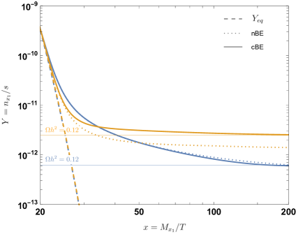
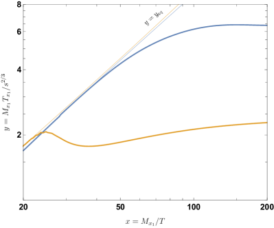
Figure 1: An example evolution of the yield $Y$ (left) and the temperature parameter $y$ (right) for two benchmark points with parameters: $M_{x_{1}}=691.38$ GeV, $M_{x_{2}}=1388.03$ GeV, $M_{H^{+}}=1388.03$ GeV, $\sin\theta=0.001264$, $\mu^{{}^{\prime\prime}}_{S}=3943.34$ GeV, $\lambda_{S12}=\lambda_{S1}=\lambda_{S2}=0$, $\lambda_{S}=\lambda_{2}=\pi$, $\lambda_{3}=0$ (blue) and $M_{x_{1}}=175.31$ GeV, $M_{x_{2}}=264.34$ GeV, $M_{H^{+}}=415.59$ GeV, $\sin\theta=5.59\times 10^{-4}$, $\mu^{{}^{\prime\prime}}_{S}=859.79$ GeV, $\lambda_{S12}=2.722$, $\lambda_{S1}=2.5\times 10^{-5}$, $\lambda_{S2}=1.163$, $\lambda_{S}=\lambda_{2}=\pi$, $\lambda_{3}=0.5759$ (orange). The solid lines give the actual thermal history as described by the cBE system, while dotted the nBE one.

In Fig. 1 we show the thermal history of two example benchmark points for which kinetic decoupling happens early enough to have an impact on the final relic abundance. The left plot shows the evolution of the yield and how it differs between the cBE and the usual approach assuming kinetic equilibrium throughout (which we call nBE), while right plot highlights how the temperature evolution can differ from the one of the SM plasma. Both example points have strong semi-annihilation and kinetic decoupling happening at a time when the annihilations are still active, thus leading to a modification of the evolution of the DM number density.

5 Phase transition and gravitational waves

The vacuum in which we live today corresponds to the minimum of the scalar potential located at the broken EW phase $(h,H,s)=(v,0,0)$. In the first moments of the Universe, however, the temperature was so large that thermal corrections influenced the $T=0$ effective potential significantly. As one goes back in time, the temperature raises and the increasing thermal effects push the low-temperature minimum (or true vacuum) upward: it becomes higher than the minimum at the origin and eventually disappears. Thus in the limit of $T\rightarrow\infty$, the high-temperature, symmetric phase is usually $(h,H,s)=(0,0,0)$; the symmetry is restored. A more complicated possibility is symmetry non-restoration, where in this limit the minimum of the potential does not go to the origin Mohapatra:1979qt ; Mohapatra:1979vr , or inverse symmetry breaking Weinberg:1974hy , where a symmetry, not broken at low temperature, is broken at high temperature.

In our case, the story thus begins at the origin of the potential, in the high-temperature phase. Then as the temperature decreases, the potential develops a second minimum, say along the $h$ axis, where the potential is initially larger than at the origin. With time, the temperature continues to decrease until these two phases become degenerate: the value of the potential in both vacua is identical. The temperature at which it occurs is the critical temperature $T_{c}$. At some lower temperature, the field will eventually tunnel from this false vacuum to a deeper stable minimum (or true vacuum), here along the $h$ axis. This tunneling occurs through the nucleation of bubbles of true vacuum, which expand and collide with each others, filling the Universe little by little and thereby gradually converting the false vacuum into the true vacuum. The collision between these bubbles is responsible for the generation of a stochastic gravitational-wave background. The temperature at which one bubble nucleates per Hubble volume is called the nucleation temperature $T_{n}$. For a fast first-order phase transition without large reheating, this can be considered as the temperature at which gravitational waves are produced Caprini:2015zlo . Finally, the value of the Higgs VEV smoothly evolves towards its tree-level value $v$ as the temperature approaches zero.

A couple of important parameters capture the most information about a first-order phase transition. The strength of a first-order phase transition is characterized by the vacuum energy $\Delta\epsilon$ released during the phase transition. To obtain a dimensionless parameter $\alpha$, one normalizes this vacuum energy to the energy density of the plasma outside the bubbles $\rho_{\text{rad}}$ Espinosa:2010hh :

$$\alpha\equiv\frac{\Delta\epsilon}{\rho_{\text{rad}}}\Big{|}_{T=T_{*}},\quad\Delta\epsilon\equiv\epsilon\big{|}_{\text{false vacuum}}-\epsilon\big{|}_{\text{true vacuum}}$$ (65)

with $\epsilon=V_{\rm eff}-\frac{T}{4}\frac{\partial V_{\rm eff}}{\partial T}$, $T_{*}$ the temperature at which GWs are generated and $\rho_{\text{rad}}=\frac{\pi^{2}}{30}g_{*}T^{4}$, where $g_{*}$ is the effective number of relativistic degrees of freedom at the temperature $T$. Note that a first-order phase transition is characterized as a strong one if the ratio of the VEV to the temperature, evaluated at $T_{*}$, satisfies

$$\frac{v_{*}}{T_{*}}\geq 1.$$ (66)

The inverse time duration of the PT, $\beta$, is usually normalized by the Hubble parameter $H_{*}\equiv H(T_{*})$ Grojean:2006bp :

$$\frac{\beta}{H_{*}}=T\frac{d(S/T)}{dT}\Big{|}_{T=T_{*}},$$ (67)

where $S\equiv S(h,H,s,T)$ is the 3-dimensional Euclidean action computed for an $O(3)$-symmetric critical bubble. A large $\beta/H_{*}$ means that we can safely neglect the Hubble expansion of the Universe during the phase-transition process.

A single bubble cannot generate gravitational waves, because its quadrupole moment vanishes due of its spherical symmetry. The key ingredient for a stochastic GW background to be generated is the collisions between these bubbles of true vacuum, as mentioned above. Indeed this will break the spherical symmetry of each of the collided scalar-field bubbles Kamionkowski:1993fg . For bubbles evolving in a thermal plasma, additional contributions to the GW signal come from the metric perturbation induced by the plasma: sound waves Hogan:1986qda ; Hindmarsh:2013xza and magnetohydrodynamic (MHD) turbulence Caprini:2009yp . Sub- and supersonic bubbles, respectively, create compression waves beyond the bubble wall and rarefaction waves behind it. When acoustic waves from different bubbles overlap, the induced shear stress of the metric generate gravitational waves. Finally, bubble collision is responsible for the turbulent motion of the fully ionized plasma. These MHD turbulences will generate gravitational waves. The power spectrum $h^{2}\Omega_{\text{GW}}$ of the stochastic GW background from a cosmic phase transitions thus arises from three contributions Caprini:2015zlo : $h^{2}\Omega_{\text{GW}}\simeq h^{2}\Omega_{\text{col}}+h^{2}\Omega_{\text{sw}}+h^{2}\Omega_{\text{turb}}$.

The scalar-field contribution redshifted to today is given in the envelope approximation by Huber:2008hg

$$h^{2}\Omega_{\text{col}}(f)=h^{2}\Omega_{\text{col}}^{\text{peak}}S_{\text{col}}(f),$$ (68)

with

$$\begin{split}h^{2}\Omega_{\text{col}}^{\text{peak}}&=1.67\times 10^{-5}\left(\frac{H_{*}}{\beta}\right)^{2}\left(\frac{\kappa_{\text{col}}\alpha}{1+\alpha}\right)^{2}\left(\frac{100}{g_{*}}\right)^{1/3}\left(\frac{0.11v_{w}^{3}}{0.42+v_{w}^{2}}\right),\\ \quad S_{\text{col}}&=\frac{3.8\left(f/f_{\text{col}}\right)^{2.8}}{1+2.8\left(f/f_{\text{col}}\right)^{3.8}},\end{split}$$ (69)

where $\kappa_{\text{col}}$ is the efficiency factor for the conversion of the vacuum energy into the gradient energy of the scalar field (energy stored in the shell of the scalar-field bubbles), $v_{w}$ is the bubble-wall speed in the rest frame of the plasma far away from the bubble Caprini:2015zlo and $f_{\text{col}}$ is the peak frequency, thus the frequency at $h^{2}\Omega_{\text{col}}^{\text{peak}}$.

The sound-wave contribution is given by Hindmarsh:2017gnf ; Caprini:2019egz ; Schmitz:2020rag

$$h^{2}\Omega_{\text{sw}}(f)=h^{2}\Omega_{\text{sw}}^{\text{peak}}S_{\text{sw}}(f),$$ (70)

with

$$\begin{split}h^{2}\Omega_{\text{sw}}^{\text{peak}}&=1.23\times 10^{-6}\left(\frac{H_{*}}{\beta}\right)\left(\frac{\kappa_{\text{sw}}\alpha}{1+\alpha}\right)^{2}\left(\frac{100}{g_{*}}\right)^{1/3}v_{w}\Upsilon,\\ S_{\text{sw}}&=\left(\frac{f}{f_{\text{sw}}}\right)^{3}\left(\frac{7}{4+3\left(f/f_{\text{sw}}\right)^{2}}\right)^{7/2},\end{split}$$ (71)

where $\kappa_{\text{sw}}$ is the efficiency factor for the conversion of the vacuum energy into the bulk motion of the plasma and $f_{\text{sw}}$ is the sound-wave peak frequency. The suppression factor for a radiation-dominated Universe is defined as Guo:2020grp ; Ellis:2019oqb

$$\Upsilon=1-\frac{1}{\sqrt{2\tau_{\text{sw}}H+1}},$$ (72)

where $\tau_{\text{sw}}$ is the time after which sound waves do not source the GW production and where $\Upsilon\simeq\tau_{\text{sw}}H$ when $\tau_{\text{sw}}H\ll 1$, thus when this time is much smaller than a Hubble time.

Finally, the MHD-turbulence contribution is given by Caprini:2015zlo ; Schmitz:2020syl

$$h^{2}\Omega_{\text{turb}}(f)=h^{2}\Omega_{\text{turb}}^{\text{peak}}S_{\text{turb}}(f),$$ (73)

with

$$h^{2}\Omega_{\text{turb}}^{\text{peak}} =3.35\times 10^{-4}\left(\frac{H_{*}}{\beta}\right)\left(\frac{\kappa_{\text{turb}}\alpha}{1+\alpha}\right)^{3/2}\left(\frac{100}{g_{*}}\right)^{1/3}v_{w}\left[\frac{1}{2^{11/3}\left(1+8\pi f_{\text{turb}}/h_{*}\right)}\right],$$ (74)

$$S_{\text{turb}} =\frac{\left(f/f_{\text{turb}}\right)^{3}}{\left[1+\left(f/f_{\text{turb}}\right)\right]^{11/3}}\left[\frac{2^{11/3}\left(1+8\pi f_{\text{turb}}/h_{*}\right)}{1+8\pi f/h_{*}}\right],$$ (75)

where $\kappa_{\text{turb}}$ is the efficiency factor for the conversion of the vacuum energy into the MHD turbulences, $f_{\text{turb}}$ is the MHD-turbulence peak frequency and $h_{*}$ is the today-redshifted value of the Hubble rate at $T_{*}$.

6 Numerical scan

We used Markov Chain Monte Carlo (MCMC) with the Metropolis-Hastings algorithm in order to generate points, starting with a number of points with the DM relic density within the Planck $3\sigma$ range. We then imposed other constraints: perturbativity, perturbative unitarity, bounded-from-below conditions for the scalar potential, globality of the EW vacuum, bounds on electroweak precision parameters $S$, $T$ and $U$, Higgs invisible width and Higgs to diphoton $h\to\gamma\gamma$ decay.

We performed three scans:

1. Points with non-zero quartic $\lambda_{S12}$ coupling (and $\mu^{\prime\prime}_{S}=\lambda_{S1}=\lambda_{S2}=\lambda_{3}=0$)

2. Points with non-zero cubic $\mu^{\prime\prime}_{S}$ coupling (and $\lambda_{S12}=\lambda_{S1}=\lambda_{S2}=\lambda_{3}=0$)

3. General points with non-zero $\mu^{\prime\prime}_{S}$ and $\lambda_{S12}$ and without conditions on the quartic portals $\lambda_{S1}$, $\lambda_{S2}$, $\lambda_{3}$.

In the first two cases, all the biquadratic portal couplings were set to zero, i.e. $\lambda_{S1}=\lambda_{S2}=\lambda_{3}=0$, except for $\lambda_{4}$, because this would have entailed enforcing a special relation between $M_{x_{2}}$ and $M_{H^{\pm}}$. Since we need a non-zero mixing angle $\theta$ between $x_{1}$ and $x_{2}$, the $\mu_{SH}$ mixing term was non-zero in all cases. The dark sector scalar self-couplings were set to $\lambda_{S}=\lambda_{2}=\pi$ in order to allow for larger values of $\lambda_{S12}$ and $\mu^{\prime\prime}_{S}$ which are otherwise constrained by vacuum stability.

New points were generated from a multivariate normal distribution. The initial covariance matrix was calculated from a set of a few tens of points with DM relic density within the Planck $3\sigma$ bounds. The initial values for $M_{x_{2}}$ and $M_{H^{\pm}}$ were chosen in an interval around $2M_{x_{1}}$ in order to enhance semi-annihilation processes. The covariance matrix was updated with each added point, while its norm was kept constant to ensure a reasonable acceptance ratio of points. Dimensionful quantities $M_{x_{1}}$, $M_{x_{2}}$, $M_{H^{\pm}}$ and $\mu^{\prime\prime}_{S}$ were generated logarithmically and only points with $M_{x_{1}}<M_{x_{2}},M_{H^{\pm}}$ kept. Similarly to the calculation of the initial distribution, a few tens of points with DM relic density within the Planck $3\sigma$ bounds and varied couplings were used to start the MCMC chains from a few hundred up to thousand points in length. Since the desired probability distributions of our MCMCs were rather arbitrary, we do not consider the density of points in our plots to have a specific statistical meaning.

The desired distribution for each case consists of a product of Gaussians whose central values and standard deviations are given in Table 1. Extra suppression factors of an arbitrary small value $10^{-12}$ were used to make the Gaussians essentially one-sided when the conditions $\sin\theta>0$ and $0\leq\lambda_{S12}<4$ (the maximal value from vacuum stability bounds for $\lambda_{S}=\lambda_{2}=\pi$ and portal couplings $\lambda_{S1}=\lambda_{S2}=\lambda_{3}=0$), and $1\leq\mu^{\prime\prime}_{S}/\text{GeV}<2\sqrt{\lambda_{S}}M_{x_{1}}/\text{GeV}$ did not hold true. In the last condition, used in the second and third scans, we limited the cubic coupling by $|\mu^{\prime\prime}_{S}|<2\sqrt{\lambda_{S}}M_{x_{1}}$, the bound from absolute vacuum stability in the $\mathbb{Z}_{3}$ singlet limit. Notice that unlike in the singlet-only limit, the cubic $\mu^{\prime\prime}_{S}$ coupling can yield semi-annihilation together with the ever-present mixing term $\mu_{SH}$.

Table 1: The central values and standard deviations for the desired distribution of the MCMC.

Quantity	Central value	Standard deviation
$\Omega_{c}h^{2}$	$0.120$	$0.001$
$M_{x_{1}}/\text{GeV}$	$333.33$	500
$M_{x_{2}}/\text{GeV}$	$2M_{x_{1}}/\text{GeV}$	250
$M_{H^{\pm}}/\text{GeV}$	$2M_{x_{1}}/\text{GeV}$	250
$\sin\theta$	$0$	$0.125$
$|M_{x_{2}}-M_{H^{\pm}}|/\text{GeV}$	0	360
$\mu^{\prime\prime}_{S}/\text{GeV}$	$2\sqrt{\lambda_{S}}M_{x_{1}}/\text{GeV}$	$\frac{1}{3}\times 2\sqrt{\lambda_{S}}M_{x_{1}}/\text{GeV}$

7 Signals

We now discuss the results of the scan, in particular for the direct-detection and gravitational-wave signals.

7.1 Direct detection

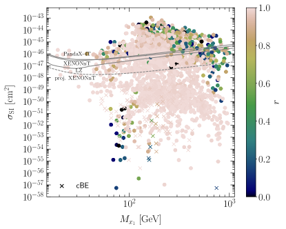
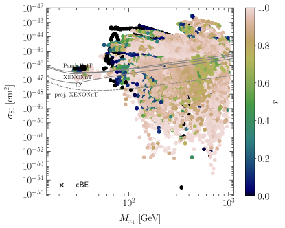
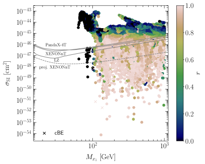
Figure 2: Spin-independent direct detection cross section vs. dark matter mass. Top panel: points dominated by $\lambda_{S12}$; middle panel: points dominated by $\mu^{\prime\prime}_{S}$ and $\mu_{SH}$; bottom panel: more general points. Also shown are the sensitivity curves of the XENON1T (2018) XENON:2018voc , PandaX-4T (2021) PandaX-4T:2021bab , LZ (2022) LZ:2022ufs in grey and the projected sensitivity curve for XENONnT XENON:2020kmp in dashed grey.

In Fig. 2 we show the predictions for the spin-independent direct detection cross section for the three cases. The top panel shows points with non-zero $\lambda_{S12}$, the middle panel points dominated by $\mu^{\prime\prime}_{S}$ and the bottom panel shows the points from the more general scan. Also shown are the sensitivity curves of the XENON1T (2018) XENON:2018voc , PandaX-4T (2021) PandaX-4T:2021bab , LZ (2022) LZ:2022ufs in grey and the projected sensitivity curve for XENONnT XENON:2020kmp in dashed grey. The color code shows the semi-annihilation fraction $r$ defined by

$$r=\frac{1}{2}\frac{v\sigma_{xx\to x^{*}X}}{v\sigma_{xx^{*}\to XX}+\frac{1}{2}\sigma_{xx\to x^{*}X}},$$ (76)

where $x$ denotes $x_{1}$, $x_{2}$, $H^{\pm}$ and $X$ stands for any SM particles. With dominant semi-annihilation $r$ approaches unity. The points with early kinetic decoupling, evaluated with the cBE method detailed in Section 4, are marked with crosses.

7.2 Gravitational waves

For each of the three scans mentioned in Section 6, we study how the Universe ends in the EW vacuum $(v,0,0)$ at zero temperature. If at least one phase transition, to reach that state, is of the first order, then we subsequently compute the power spectrum of the stochastic GW background $h^{2}\Omega_{\text{GW}}$, necessarily associated to these cosmic FOPTs. In addition to the previous constraints, we also take into account the constraint from direct-detection experiments: only points not excluded by LZ are displayed in Fig. 3 and Fig. 4.

In the left panel of Fig. 3, we show, for the three scans, the region of the parameter space, projected onto the plane made by the mixing angle $\sin\theta$ and the DM mass $M_{x_{1}}$, that gives rise to first-order phase transitions. These are essentially obtained for large mixing and mild to large DM mass. We see that only points from the general scan lead to strong FOPTs. The right panel shows the values of either $\lambda_{S12}$ or $\mu_{S}^{\prime\prime}$, as a function of $M_{x_{1}}$, responsible for FOPTs for scans where they are non-zero. In both panels, triangles are points for which the cBE method has been used to compute the DM relic density, as the scattering rate is not sufficient to consider kinetic equilibrium for DM during the freeze-out process (see Section 4).

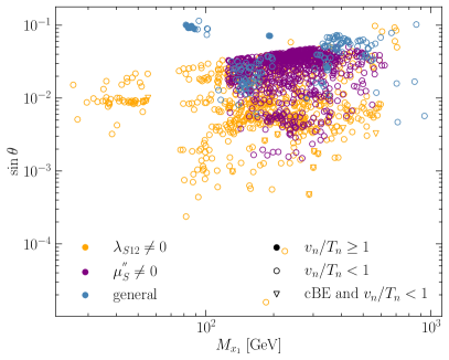
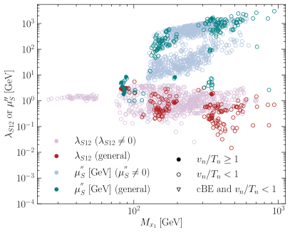
Figure 3: Projection of the parameter space, showing points which satisfy all the theoretical/experimental constraints. cBE points that lead to FOPT are only found for $\lambda_{S12}\neq 0$ scan. Strong FOPT are only found for general scan. Left panel: Sine of the mixing angle $\sin\theta$ vs. DM mass $M_{x_{1}}$. Right panel: $\lambda_{S12}$ vs. $M_{x_{1}}$ for both the $\lambda_{S12}\neq 0$ and general scan and $\mu_{S}^{\prime\prime}$ vs. $M_{x_{1}}$ for both the $\mu^{\prime\prime}_{S}\neq 0$ and general scan.

The signal from the stochastic gravitational-wave background is shown in Fig. 4, with the power-law integrated (PLI) sensitivity curves of LISA, DECIGO and BBO, obtained for an observation time of 4 years and a threshold value for the signal-to-noise ratio to be 10 Thrane:2013oya ; Azatov:2019png . Similarly to Fig. 2, we show the semi-annihilation fraction with a color code. The upper panel of Fig. 4 shows the GW signal for the scan with non-zero $\lambda_{S12}$. This signal results from single-step FOPTs. We can see that none of the points leads to strong FOPTs and that for some of them (triangles), the assumption of kinetic equilibrium does not hold and the full cBE system should be solved. The middle panel shows the GW signal for the scan with non-zero $\mu^{\prime\prime}_{S}$. Again, we only find single-step weak FOPTs. A cubic term helps to generate a barrier in the potential and thus enhance the strength of the phase transition. However, we only find a single-step FOPT from the origin towards the EW minimum, thereby along the Higgs direction $h$. This is why a non-zero $\mu^{\prime\prime}_{S}$ is not helpful here to obtain a stronger PT, as it only impacts the $s$ direction. Finally, the lower panel of Fig. 4 shows the GW signal for the general scan, where strong FOPTs are obtained and where one of the points clearly lies above the LISA PLI sensitivity curve, thus yielding a detectable GW signal. Note that we also found two-step phase transitions. For each of them, indicated by a triangle, the first step $(0,0,0)\rightarrow(0,v_{H},0)$ is a second-order PT and is followed by a first-order PT $(0,v_{H}^{{}^{\prime}},0)\rightarrow(v_{h},0,0)$. Note also that from Fig. 4, it seems that the lower the semi-annihilation fraction, the stronger the GW signal. However, if we do not take experimental constraints into account, the correlation between the strength of the GW signal and the semi-annihilation fraction is lost.

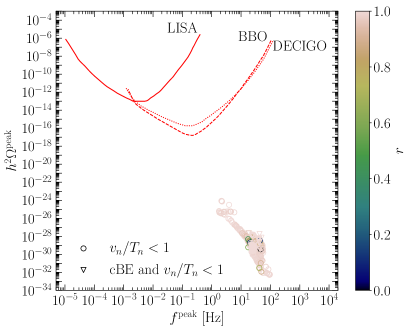
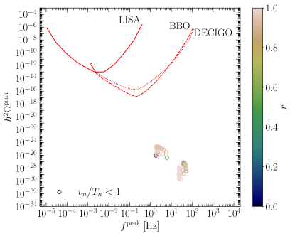
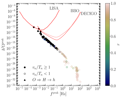
Figure 4: Peak amplitude of the GW signal as a function of peak frequency. The top panel shows points with non-zero $\lambda_{S12}$, the middle panel points dominated by $\mu^{\prime\prime}_{S}$ and the bottom panel shows the points from the more general scan. Also shown are the PLI sensitivity curves of future detectors LISA, BBO and DECIGO.

Finally, let us stress that in principle, in this model, if we relax the constraint on relic density and allow for underabundant DM, we can more easily find regions of the parameter space allowing for different kind of multi-step phase transitions in the three-dimensional field space $(h,H,s)$ and/or leading to a strong enough GW signal to be detected by LISA, DECIGO or BBO, as can be seen in Fig. 5. The points in this figure comply with all the theoretical/experimental constraints, except that they only lead to underabundant DM, and result from a random scan in the following range:

$$M_{x_{1}} \in[10,1000]\text{~{}GeV}, M_{x_{2}},M_{H^{\pm}} \in[M_{x_{1}},1000\text{~{}GeV}], \sin\theta \in[0,\sqrt{2}/2],$$

$$\mu^{\prime\prime}_{S} \in[0,2000]\text{~{}GeV}, \lambda_{3},\lambda_{S1},\lambda_{S2},\lambda_{S12} \in[-4\pi,4\pi], \lambda_{2},\lambda_{S} \in[-\pi,4\pi].$$ (77)

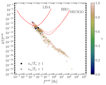
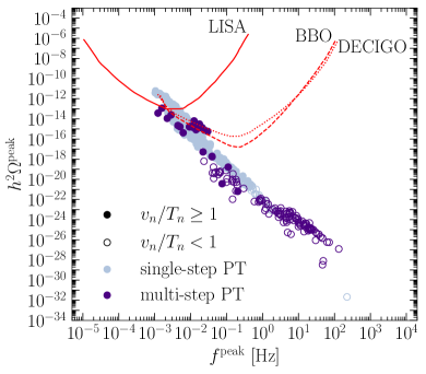
Figure 5: Peak amplitude of the GW signal as a function of peak frequency with points from the scan in Eq. (7.2). Also shown are the PLI sensitivity curves of future detectors LISA, BBO and DECIGO. The left panel highlights the semi-annihilation rate, while the right panel distinguishes single-step from multi-step PTs.

8 Conclusions

We have explored the cosmology of the $\mathbb{Z}_{3}$ symmetric dark matter model with an inert doublet and a complex singlet with the emphasis on detectability of the gravitational-wave signal and dark-matter phenomenology. In order for the model to be in agreement with direct-detection limits the dark matter candidate needs to be a singlet-like state arising from the mixing of the singlet and the neutral part of the inert doublet. This setup opens an interesting possibility of important or even dominant semi-annihilation processes that modifies the thermal DM production through an early kinetic decoupling: if the relic density is determined via semi-annihilation, the dark matter-Higgs boson couplings that would keep DM in kinetic equilibrium via elastic collisions are suppressed.

We performed MCMC scans to not only produce general coupling configurations available to the model, but also to look specifically at large semi-annihilation (through a large cubic coupling $\mu^{\prime\prime}_{S}$ or the quartic semi-annihilation coupling $\lambda_{S12}$ coupling). We find that for the points with dominant semi-annihilation, strong suppression of the direct-detection signal comes also with weak FOPTs whose GW signals would lie orders of magnitude below detection projections in a foreseeable future. On the other hand, a general scan of the model reveals points near the detection limits of LISA, DECIGO and BBO.

We then also computed the GW signal for uniformly distributed random general scan allowing for underabundant singlet-like $x_{1}$ with relic density below the Planck constraint. (There could be either an additional non-thermal production mechanism or another DM component.) In that case we found a sizable portion of the parameter space leading to a single-step or a multi-step phase transition producing strong enough GW signal to be potentially detected by LISA, DECIGO or BBO.

Therefore, we conclude that in the $\mathbb{Z}_{3}$ symmetric model with an inert doublet and a complex singlet there exists a parameter range that explaining whole dark matter and providing potentially observable GW peak amplitude, though it is rather small and challenging to be observed in the near future. Nevertheless, when extending the analysis to underabundant dark matter the detection prospects of the GW peak amplitude become significantly more promising.

Appendix A Field-dependent scalar mass matrices

The field-dependent scalar masses $m_{i}^{2}\equiv m_{i}^{2}(h,H,s)$, present in Eq. (6) and Eq. (10), correspond to the eigenvalues of the field-dependent mass matrices of the scalar fields $M^{2}_{S}$, of the pseudoscalar fields $M^{2}_{P}$ and of the charged fields $M^{2}_{C}$:

$$M_{S}^{2} ={\footnotesize\begin{pmatrix}\mu_{1}^{2}+3\lambda_{1}h^{2}+\frac{\lambda_{3}+\lambda_{4}}{2}H^{2}+\frac{\lambda_{S1}}{2}s^{2}&(\lambda_{3}+\lambda_{4})hH+\frac{\lambda_{S12}s+\sqrt{2}\mu_{SH}}{4}s&\lambda_{S1}hs+\frac{\lambda_{S12}}{2}Hs+\frac{\sqrt{2}\mu_{SH}}{4}H\\ (\lambda_{3}+\lambda_{4})hH+\frac{\lambda_{S12}s+\sqrt{2}\mu_{SH}}{4}s&\mu_{2}^{2}+3\lambda_{2}H^{2}+\frac{\lambda_{3}+\lambda_{4}}{2}h^{2}+\frac{\lambda_{S2}}{2}s^{2}&\lambda_{S2}Hs+\frac{\lambda_{S12}}{2}hs+\frac{\sqrt{2}\mu_{SH}}{4}h\\ \lambda_{S1}hs+\frac{\lambda_{S12}}{2}Hs+\frac{\sqrt{2}\mu_{SH}}{4}H&\lambda_{S2}Hs+\frac{\lambda_{S12}}{2}hs+\frac{\sqrt{2}\mu_{SH}}{4}h&\mu_{S}^{2}+3\lambda_{S}s^{2}+\frac{3}{\sqrt{2}}\mu^{\prime\prime}_{S}s\\ &&+\frac{\lambda_{S1}h^{2}+\lambda_{S2}H^{2}+\lambda_{S12}hH}{2}\end{pmatrix}},$$ (78)

$$M_{P}^{2} ={\footnotesize\begin{pmatrix}\mu_{1}^{2}+\lambda_{1}h^{2}+\frac{\lambda_{3}+\lambda_{4}}{2}H^{2}+\frac{\lambda_{S1}}{2}s^{2}&\frac{\lambda_{S12}s+\sqrt{2}\mu_{SH}}{4}s&\frac{\lambda_{S12}}{2}Hs-\frac{\sqrt{2}\mu_{SH}}{4}H\\ \frac{\lambda_{S12}s+\sqrt{2}\mu_{SH}}{4}s&\mu_{2}^{2}+\lambda_{2}H^{2}+\frac{\lambda_{3}+\lambda_{4}}{2}h^{2}+\frac{\lambda_{S2}}{2}s^{2}&-\frac{\lambda_{S12}}{2}hs+\frac{\sqrt{2}\mu_{SH}}{4}h\\ \frac{\lambda_{S12}}{2}Hs-\frac{\sqrt{2}\mu_{SH}}{4}H&-\frac{\lambda_{S12}}{2}hs+\frac{\sqrt{2}\mu_{SH}}{4}h&\mu_{S}^{2}+\lambda_{S}s^{2}-\frac{3}{\sqrt{2}}\mu^{\prime\prime}_{S}s\\ &&+\frac{\lambda_{S1}h^{2}+\lambda_{S2}H^{2}-\lambda_{S12}hH}{2}\end{pmatrix}},$$ (79)

$$M_{C}^{2} =\begin{pmatrix}\mu_{1}^{2}+\lambda_{1}h^{2}+\frac{\lambda_{3}}{2}H^{2}+\frac{\lambda_{S1}}{2}s^{2}&\frac{\lambda_{4}}{2}hH+\frac{\lambda_{S12}s+\sqrt{2}\mu_{SH}}{4}s\\ \frac{\lambda_{4}}{2}hH+\frac{\lambda_{S12}s+\sqrt{2}\mu_{SH}}{4}s&\mu_{2}^{2}+\lambda_{2}H^{2}+\frac{\lambda_{3}}{2}h^{2}+\frac{\lambda_{S2}}{2}s^{2}\end{pmatrix}.$$ (80)

Evaluated in the EW vacuum $(h,H,s)=(v,0,0)$, these mass matrices become

$$M_{S}^{2} =\begin{pmatrix}\mu_{1}^{2}+3\lambda_{1}v^{2}&0&0\\ 0&\mu_{2}^{2}+\frac{\lambda_{3}+\lambda_{4}}{2}v^{2}&\frac{\sqrt{2}\mu_{SH}}{4}v\\ 0&\frac{\sqrt{2}\mu_{SH}}{4}v&\mu_{S}^{2}+\frac{\lambda_{S1}v^{2}}{2}\end{pmatrix},$$ (81)

$$M_{P}^{2} =\begin{pmatrix}\mu_{1}^{2}+\lambda_{1}v^{2}&0&0\\ 0&\mu_{2}^{2}+\frac{\lambda_{3}+\lambda_{4}}{2}v^{2}&\frac{\sqrt{2}\mu_{SH}}{4}v\\ 0&\frac{\sqrt{2}\mu_{SH}}{4}v&\mu_{S}^{2}+\frac{\lambda_{S1}v^{2}}{2}\end{pmatrix},$$ (82)

$$M_{C}^{2} =\begin{pmatrix}\mu_{1}^{2}+\lambda_{1}h^{2}&0\\ 0&\mu_{2}^{2}+\frac{\lambda_{3}}{2}v^{2}\end{pmatrix},$$ (83)

thus putting in evidence the mixing between $H_{2}$ and $S$.

Appendix B Counter-terms

We present expressions for counter-terms in the effective potential used to keep VEVs, masses and mixing at their tree-level values. Since the counter-terms $\delta\lambda_{3}$ and $\delta\lambda_{4}$ only appear as a sum in Eq. (8), we can arbitrarily set $\delta\lambda_{4}$ to zero. The counter-terms, expressed via derivatives of the one-loop Coleman-Weinberg potential (6), are given by

$$\delta\mu_{1}^{2} =\frac{v\partial_{h}^{2}\Delta V-3\partial_{h}\Delta V}{4v},$$ (84)

$$\delta\mu_{2}^{2} =\frac{v\partial_{h}\partial_{H^{0}}^{2}V-2\partial_{H^{0}}^{2}\Delta V}{4},$$ (85)

$$\delta\mu_{S}^{2} =\frac{v\partial_{h}\partial_{s_{R}}^{2}V-2\partial_{s_{R}}^{2}\Delta V}{4},$$ (86)

$$\delta\mu_{SH} =-\partial_{H^{0}}\partial_{s_{R}}\Delta V,$$ (87)

$$\delta\mu^{\prime\prime}_{S} =-\frac{1}{6}\partial_{s_{R}}^{3}\Delta V,$$ (88)

$$\delta\lambda_{1} =\frac{\partial_{h}\Delta V-v\partial_{h}^{2}\Delta V}{8v^{3}},$$ (89)

$$\delta\lambda_{3} =-\frac{1}{4v}\partial_{h}\partial_{H^{0}}^{2}\Delta V,$$ (90)

$$\delta\lambda_{S1} =-\frac{1}{4v}\partial_{h}\partial_{s_{R}}^{2}\Delta V,$$ (91)

$$\delta\lambda_{S12} =-\frac{1}{2v}\partial_{H^{0}}\partial_{s_{R}}^{2}\Delta V.$$ (92)

Appendix C Sound-wave contribution $h^{2}\Omega_{\text{sw}}(f)$

From Hindmarsh:2017gnf ; Caprini:2019egz ; Schmitz:2020rag one has

$$h^{2}\Omega_{\text{sw}}^{\text{peak}}=3h^{2}\times 0.687F_{\text{gw,0}}\Gamma^{2}\bar{U}_{f}^{4}\frac{H_{*}R_{*}}{c_{s}}\tilde{\Omega}_{\text{gw}}\Upsilon,$$ (93)

where the mean adiabatic index $\Gamma=4/3$ for a relativistic fluid, and the enthalpy-weighted root-mean-square of the fluid velocity $\bar{U}_{f}$ is expressed as Schmitz:2020rag :

$$\bar{U}_{f}=\sqrt{\frac{K}{\Gamma}},\quad K=\frac{\kappa_{\text{sw}}\alpha}{1+\alpha}.$$ (94)

The mean bubble separation at percolation temperature $R_{*}$ is defined as

$$R_{*}=\frac{(8\pi)^{1/3}\text{max}\{c_{s},v_{w}\}}{\beta}$$ (95)

with $c_{s}=1/\sqrt{3}$ the speed of sound in the plasma Espinosa:2010hh .

The parameter $\tilde{\Omega}_{\text{gw}}$, which quantifies how efficiently the kinetic energy is converted into gravitational waves, is numerically found to be $\tilde{\Omega}_{\text{gw}}\simeq 1.2\times 10^{-2}$ Hindmarsh:2017gnf ; Schmitz:2020rag .

Finally, the factor $F_{\text{gw,0}}$ needed to obtain the today value $h^{2}\Omega_{\text{sw}}^{\text{peak}}$ is defined as Caprini:2019egz ; Schmitz:2020rag

$$F_{\text{gw,0}}=\Omega_{\gamma,0}\left(\frac{g_{s0}}{g_{s*}}\right)^{4/3}\frac{g_{*}}{g_{0}},$$ (96)

where $\Omega_{\gamma,0}\equiv\rho_{\gamma,0}/\rho_{c,0}$ is the photon density today, $g_{s*}$ the effective number of entropic degrees of freedom, $g_{*}$ the effective number of relativistic degrees of freedom, while $g_{s0}$ and $g_{0}$ give their present values, respectively. The degrees of freedom $g_{s*}$ and $g_{*}$ are equal at the EW scale, while $g_{s0}$ and $g_{0}$ are different since they are considered after the neutrino decoupling.

The following values for the aforementioned parameters allows us to compute the factor $F_{\text{gw,0}}$ Mulders:2019vhb ; Gelmini:1996kv :

$$\rho_{\gamma,0}=0.26~{}\frac{\text{eV}}{\text{cm}^{3}},\quad\rho_{c,0}=1.05\times 10^{-5}h^{2}~{}\text{GeV}\,\text{cm}^{-3},\quad h\equiv\frac{H_{0}}{100~{}\text{km~{}s}^{-1}\text{Mpc}^{-1}},$$

$$g_{s0}\simeq 3.94\quad\text{and}\quad g_{0}\simeq 3.38,$$ (97)

where $N_{\text{eff}}=3.044$ Akita:2022hlx has been used in the computation of $g_{s0}$ and $g_{0}$. Note that $g_{s0}\simeq 3.91$ and $g_{0}=2$ are considered in Refs. Hindmarsh:2017gnf ; Caprini:2019egz . Considering these values, we can thus express $F_{\text{gw,0}}$ as

$$F_{\text{gw,0}}=\frac{9.77\times 10^{-6}}{h^{2}}\left(\frac{100}{g_{*}}\right)^{1/3}$$ (98)

Putting all together, we finally obtain

$$h^{2}\Omega_{\text{sw}}^{\text{peak}} =2.061h^{2}\frac{9.77\times 10^{-6}}{h^{2}}\left(\frac{100}{g_{*}}\right)^{1/3}\left(\frac{\kappa_{\text{sw}}\alpha}{1+\alpha}\right)^{2}\frac{H_{*}(8\pi)^{1/3}\text{max}\{c_{s},v_{w}\}}{\beta/\sqrt{3}}1.2\times 10^{-2}~{}\Upsilon$$

$$\simeq 1.23\times 10^{-6}\left(\frac{H_{*}}{\beta}\right)\left(\frac{\kappa_{\text{sw}}\alpha}{1+\alpha}\right)^{2}\left(\frac{100}{g_{*}}\right)^{1/3}\text{max}\{c_{s},v_{w}\}~{}\Upsilon.$$ (99)

References

- (1) Planck collaboration, Planck 2018 results. VI. Cosmological parameters, Astron. Astrophys. 641 (2020) A6 [1807.06209].
- (2) CMS collaboration, Observation of a New Boson at a Mass of 125 GeV with the CMS Experiment at the LHC, Phys. Lett. B 716 (2012) 30 [1207.7235].
- (3) ATLAS collaboration, Observation of a new particle in the search for the Standard Model Higgs boson with the ATLAS detector at the LHC, Phys. Lett. B 716 (2012) 1 [1207.7214].
- (4) E. Ma, Verifiable radiative seesaw mechanism of neutrino mass and dark matter, Phys. Rev. D 73 (2006) 077301 [hep-ph/0601225].
- (5) L. Lopez Honorez, E. Nezri, J. F. Oliver and M. H. G. Tytgat, The Inert Doublet Model: An Archetype for Dark Matter, JCAP 02 (2007) 028 [hep-ph/0612275].
- (6) N. G. Deshpande and E. Ma, Pattern of Symmetry Breaking with Two Higgs Doublets, Phys. Rev. D 18 (1978) 2574.
- (7) R. Barbieri, L. J. Hall and V. S. Rychkov, Improved naturalness with a heavy Higgs: An Alternative road to LHC physics, Phys. Rev. D 74 (2006) 015007 [hep-ph/0603188].
- (8) V. Silveira and A. Zee, SCALAR PHANTOMS, Phys. Lett. B 161 (1985) 136.
- (9) J. McDonald, Gauge singlet scalars as cold dark matter, Phys. Rev. D 50 (1994) 3637 [hep-ph/0702143].
- (10) C. P. Burgess, M. Pospelov and T. ter Veldhuis, The Minimal model of nonbaryonic dark matter: A Singlet scalar, Nucl. Phys. B 619 (2001) 709 [hep-ph/0011335].
- (11) XENON collaboration, Dark Matter Search Results from a One Ton-Year Exposure of XENON1T, Phys. Rev. Lett. 121 (2018) 111302 [1805.12562].
- (12) PandaX-4T collaboration, Dark Matter Search Results from the PandaX-4T Commissioning Run, Phys. Rev. Lett. 127 (2021) 261802 [2107.13438].
- (13) LZ collaboration, First Dark Matter Search Results from the LUX-ZEPLIN (LZ) Experiment, 2207.03764.
- (14) T. Hambye and M. H. Tytgat, Confined hidden vector dark matter, Phys.Lett. B683 (2010) 39 [0907.1007].
- (15) T. Hambye, Hidden vector dark matter, JHEP 0901 (2009) 028 [0811.0172].
- (16) F. D’Eramo, M. McCullough and J. Thaler, Multiple Gamma Lines from Semi-Annihilation, JCAP 1304 (2013) 030 [1210.7817].
- (17) F. D’Eramo and J. Thaler, Semi-annihilation of Dark Matter, JHEP 1006 (2010) 109 [1003.5912].
- (18) G. Belanger, K. Kannike, A. Pukhov and M. Raidal, Impact of semi-annihilations on dark matter phenomenology - an example of symmetric scalar dark matter, JCAP 04 (2012) 010 [1202.2962].
- (19) G. Bélanger, K. Kannike, A. Pukhov and M. Raidal, Minimal semi-annihilating scalar dark matter, JCAP 06 (2014) 021 [1403.4960].
- (20) M. Kadastik, K. Kannike, A. Racioppi and M. Raidal, Implications of Dark Matter direct detection results on LHC physics, Phys. Lett. B 694 (2010) 242 [0912.3797].
- (21) M. Kadastik, K. Kannike and M. Raidal, Matter parity as the origin of scalar Dark Matter, Phys. Rev. D 81 (2010) 015002 [0903.2475].
- (22) M. Kadastik, K. Kannike and M. Raidal, Dark Matter as the signal of Grand Unification, Phys. Rev. D 80 (2009) 085020 [0907.1894].
- (23) M. Kadastik, K. Kannike, A. Racioppi and M. Raidal, EWSB from the soft portal into Dark Matter and prediction for direct detection, Phys. Rev. Lett. 104 (2010) 201301 [0912.2729].
- (24) M. Aoki and T. Toma, Impact of semi-annihilation of symmetric dark matter with radiative neutrino masses, JCAP 09 (2014) 016 [1405.5870].
- (25) M. Kakizaki, A. Santa and O. Seto, Phenomenological signatures of mixed complex scalar WIMP dark matter, Int. J. Mod. Phys. A 32 (2017) 1750038 [1609.06555].
- (26) G. Belanger, A. Mjallal and A. Pukhov, Two dark matter candidates: The case of inert doublet and singlet scalars, Phys. Rev. D 105 (2022) 035018 [2108.08061].
- (27) G. Belanger, A. Mjallal and A. Pukhov, WIMP and FIMP dark matter in the inert doublet plus singlet model, 2205.04101.
- (28) C. E. Yaguna and O. Zapata, Multi-component scalar dark matter from a symmetry: a systematic analysis, JHEP 03 (2020) 109 [1911.05515].
- (29) A. Bas i Beneito, J. Herrero-García and D. Vatsyayan, Multi-component dark sectors: symmetries, asymmetries and conversions, JHEP 22 (2020) 075 [2207.02874].
- (30) C. E. Yaguna and O. Zapata, Two-component scalar dark matter in Z2n scenarios, JHEP 10 (2021) 185 [2106.11889].
- (31) D. Jurčiukonis and L. Lavoura, The centers of discrete groups as stabilizers of Dark Matter, 2210.12133.
- (32) G. Bélanger, A. Pukhov, C. E. Yaguna and O. Zapata, The Z7 model of three-component scalar dark matter, JHEP 03 (2023) 100 [2212.07488].
- (33) G. Belanger, K. Kannike, A. Pukhov and M. Raidal, Scalar Singlet Dark Matter, JCAP 01 (2013) 022 [1211.1014].
- (34) S. Bhattacharya, P. Ghosh, T. N. Maity and T. S. Ray, Mitigating Direct Detection Bounds in Non-minimal Higgs Portal Scalar Dark Matter Models, JHEP 10 (2017) 088 [1706.04699].
- (35) P. Ko and Y. Tang, Self-interacting scalar dark matter with local symmetry, JCAP 05 (2014) 047 [1402.6449].
- (36) P. Ko and Y. Tang, Galactic center -ray excess in hidden sector DM models with dark gauge symmetries: local symmetry as an example, JCAP 01 (2015) 023 [1407.5492].
- (37) S.-M. Choi and H. M. Lee, SIMP dark matter with gauged Z3 symmetry, JHEP 09 (2015) 063 [1505.00960].
- (38) E. Ma, N. Pollard, R. Srivastava and M. Zakeri, Gauge Model with Residual Symmetry, Phys. Lett. B 750 (2015) 135 [1507.03943].
- (39) K. Kannike, K. Loos and M. Raidal, Gravitational wave signals of pseudo-Goldstone dark matter in the complex singlet model, Phys. Rev. D 101 (2020) 035001 [1907.13136].
- (40) W. Cheng, X. Liu and R. Zhou, Non-minimal Coupling Inflation and Dark Matter under the Symmetry, 2206.12624.
- (41) A. Hektor, A. Hryczuk and K. Kannike, Improved bounds on singlet dark matter, JHEP 03 (2019) 204 [1901.08074].
- (42) Y. Cai and A. P. Spray, The galactic center excess from scalar semi-annihilations, JHEP 06 (2016) 156 [1511.09247].
- (43) G. Arcadi, F. S. Queiroz and C. Siqueira, The Semi-Hooperon: Gamma-ray and anti-proton excesses in the Galactic Center, Phys. Lett. B 775 (2017) 196 [1706.02336].
- (44) F. S. Queiroz and C. Siqueira, Search for Semi-Annihilating Dark Matter with Fermi-LAT, H.E.S.S., Planck, and the Cherenkov Telescope Array, JCAP 04 (2019) 048 [1901.10494].
- (45) Z. Kang, P. Ko and T. Matsui, Strong first order EWPT strong gravitational waves in Z3-symmetric singlet scalar extension, JHEP 02 (2018) 115 [1706.09721].
- (46) P. Athron, J. M. Cornell, F. Kahlhoefer, J. Mckay, P. Scott and S. Wild, Impact of vacuum stability, perturbativity and XENON1T on global fits of and scalar singlet dark matter, Eur. Phys. J. C 78 (2018) 830 [1806.11281].
- (47) B. Swiezewska and M. Krawczyk, Diphoton rate in the inert doublet model with a 125 GeV Higgs boson, Phys. Rev. D 88 (2013) 035019 [1212.4100].
- (48) M. Krawczyk, D. Sokolowska, P. Swaczyna and B. Swiezewska, Constraining Inert Dark Matter by and WMAP data, JHEP 09 (2013) 055 [1305.6266].
- (49) A. Belyaev, G. Cacciapaglia, I. P. Ivanov, F. Rojas-Abatte and M. Thomas, Anatomy of the Inert Two Higgs Doublet Model in the light of the LHC and non-LHC Dark Matter Searches, Phys. Rev. D 97 (2018) 035011 [1612.00511].
- (50) A. Belyaev, T. R. Fernandez Perez Tomei, P. G. Mercadante, C. S. Moon, S. Moretti, S. F. Novaes et al., Advancing LHC probes of dark matter from the inert two-Higgs-doublet model with the monojet signal, Phys. Rev. D 99 (2019) 015011 [1809.00933].
- (51) A. Goudelis, B. Herrmann and O. Stål, Dark matter in the Inert Doublet Model after the discovery of a Higgs-like boson at the LHC, JHEP 09 (2013) 106 [1303.3010].
- (52) M. A. Díaz, B. Koch and S. Urrutia-Quiroga, Constraints to Dark Matter from Inert Higgs Doublet Model, Adv. High Energy Phys. 2016 (2016) 8278375 [1511.04429].
- (53) N. Blinov, J. Kozaczuk, D. E. Morrissey and A. de la Puente, Compressing the Inert Doublet Model, Phys. Rev. D 93 (2016) 035020 [1510.08069].
- (54) I. F. Ginzburg, K. A. Kanishev, M. Krawczyk and D. Sokolowska, Evolution of Universe to the present inert phase, Phys. Rev. D 82 (2010) 123533 [1009.4593].
- (55) G. Gil, P. Chankowski and M. Krawczyk, Inert Dark Matter and Strong Electroweak Phase Transition, Phys. Lett. B 717 (2012) 396 [1207.0084].
- (56) D. Borah and J. M. Cline, Inert Doublet Dark Matter with Strong Electroweak Phase Transition, Phys. Rev. D 86 (2012) 055001 [1204.4722].
- (57) J. M. Cline and K. Kainulainen, Improved Electroweak Phase Transition with Subdominant Inert Doublet Dark Matter, Phys. Rev. D 87 (2013) 071701 [1302.2614].
- (58) N. Blinov, S. Profumo and T. Stefaniak, The Electroweak Phase Transition in the Inert Doublet Model, JCAP 07 (2015) 028 [1504.05949].
- (59) S. Fabian, F. Goertz and Y. Jiang, Dark matter and nature of electroweak phase transition with an inert doublet, JCAP 09 (2021) 011 [2012.12847].
- (60) N. Benincasa, L. Delle Rose, K. Kannike and L. Marzola, Multi-step phase transitions and gravitational waves in the inert doublet model, 2205.06669.
- (61) P. Gondolo and G. Gelmini, Cosmic abundances of stable particles: Improved analysis, Nucl. Phys. B360 (1991) 145.
- (62) T. Binder, T. Bringmann, M. Gustafsson and A. Hryczuk, Early kinetic decoupling of dark matter: when the standard way of calculating the thermal relic density fails, Phys. Rev. D96 (2017) 115010 [1706.07433].
- (63) M. Duch and B. Grzadkowski, Resonance enhancement of dark matter interactions: the case for early kinetic decoupling and velocity dependent resonance width, JHEP 09 (2017) 159 [1705.10777].
- (64) T. Binder, T. Bringmann, M. Gustafsson and A. Hryczuk, Dark matter relic abundance beyond kinetic equilibrium, Eur. Phys. J. C 81 (2021) 577 [2103.01944].
- (65) LIGO Scientific, Virgo collaboration, GW151226: Observation of Gravitational Waves from a 22-Solar-Mass Binary Black Hole Coalescence, Phys. Rev. Lett. 116 (2016) 241103 [1606.04855].
- (66) LIGO Scientific, Virgo collaboration, Observation of Gravitational Waves from a Binary Black Hole Merger, Phys. Rev. Lett. 116 (2016) 061102 [1602.03837].
- (67) K. Kajantie, M. Laine, K. Rummukainen and M. E. Shaposhnikov, Is there a hot electroweak phase transition at ?, Phys. Rev. Lett. 77 (1996) 2887 [hep-ph/9605288].
- (68) Y. Aoki, F. Csikor, Z. Fodor and A. Ukawa, The Endpoint of the first order phase transition of the SU(2) gauge Higgs model on a four-dimensional isotropic lattice, Phys. Rev. D 60 (1999) 013001 [hep-lat/9901021].
- (69) E. Witten, Cosmic Separation of Phases, Phys. Rev. D 30 (1984) 272.
- (70) P. J. Steinhardt, Relativistic Detonation Waves and Bubble Growth in False Vacuum Decay, Phys. Rev. D 25 (1982) 2074.
- (71) C. J. Hogan, NUCLEATION OF COSMOLOGICAL PHASE TRANSITIONS, Phys. Lett. B 133 (1983) 172.
- (72) LISA collaboration, Laser Interferometer Space Antenna, 1702.00786.
- (73) eLISA collaboration, The Gravitational Universe, 1305.5720.
- (74) J. Crowder and N. J. Cornish, Beyond LISA: Exploring future gravitational wave missions, Phys. Rev. D 72 (2005) 083005 [gr-qc/0506015].
- (75) V. Corbin and N. J. Cornish, Detecting the cosmic gravitational wave background with the big bang observer, Class. Quant. Grav. 23 (2006) 2435 [gr-qc/0512039].
- (76) W.-H. Ruan, Z.-K. Guo, R.-G. Cai and Y.-Z. Zhang, Taiji program: Gravitational-wave sources, Int. J. Mod. Phys. A 35 (2020) 2050075 [1807.09495].
- (77) W.-R. Hu and Y.-L. Wu, The Taiji Program in Space for gravitational wave physics and the nature of gravity, Natl. Sci. Rev. 4 (2017) 685.
- (78) TianQin collaboration, TianQin: a space-borne gravitational wave detector, Class. Quant. Grav. 33 (2016) 035010 [1512.02076].
- (79) N. Seto, S. Kawamura and T. Nakamura, Possibility of direct measurement of the acceleration of the universe using 0.1-Hz band laser interferometer gravitational wave antenna in space, Phys. Rev. Lett. 87 (2001) 221103 [astro-ph/0108011].
- (80) S. Kawamura et al., Current status of space gravitational wave antenna DECIGO and B-DECIGO, PTEP 2021 (2021) 05A105 [2006.13545].
- (81) S. Coleman and E. Weinberg, Radiative corrections as the origin of spontaneous symmetry breaking, Phys. Rev. D 7 (1973) 1888.
- (82) C. Delaunay, C. Grojean and J. D. Wells, Dynamics of Non-renormalizable Electroweak Symmetry Breaking, JHEP 04 (2008) 029 [0711.2511].
- (83) J. M. Cline, K. Kainulainen and M. Trott, Electroweak Baryogenesis in Two Higgs Doublet Models and B meson anomalies, JHEP 11 (2011) 089 [1107.3559].
- (84) L. Dolan and R. Jackiw, Symmetry behavior at finite temperature, Phys. Rev. D 9 (1974) 3320.
- (85) D. J. Gross, R. D. Pisarski and L. G. Yaffe, Qcd and instantons at finite temperature, Rev. Mod. Phys. 53 (1981) 43.
- (86) R. R. Parwani, Resummation in a hot scalar field theory, Phys. Rev. D 45 (1992) 4695 [hep-ph/9204216].
- (87) M. E. Carrington, Effective potential at finite temperature in the standard model, Phys. Rev. D 45 (1992) 2933.
- (88) J. M. Cline and P.-A. Lemieux, Electroweak phase transition in two Higgs doublet models, Phys. Rev. D 55 (1997) 3873 [hep-ph/9609240].
- (89) E. Braaten and R. D. Pisarski, Simple effective Lagrangian for hard thermal loops, Phys. Rev. D 45 (1992) R1827.
- (90) K. Enqvist, A. Riotto and I. Vilja, Baryogenesis and the thermalization rate of stop, Phys. Lett. B 438 (1998) 273 [hep-ph/9710373].
- (91) J. R. Espinosa, M. Quiros and F. Zwirner, On the nature of the electroweak phase transition, Phys. Lett. B 314 (1993) 206 [hep-ph/9212248].
- (92) C. Manuel, On the thermal gauge boson masses of the electroweak theory in the broken phase, Phys. Rev. D 58 (1998) 016001 [hep-ph/9801364].
- (93) J. Bernon, L. Bian and Y. Jiang, A new insight into the phase transition in the early Universe with two Higgs doublets, JHEP 05 (2018) 151 [1712.08430].
- (94) R. N. Lerner and J. McDonald, Gauge singlet scalar as inflaton and thermal relic dark matter, Phys. Rev. D 80 (2009) 123507 [0909.0520].
- (95) S. Kanemura, T. Kubota and E. Takasugi, Lee-Quigg-Thacker bounds for Higgs boson masses in a two doublet model, Phys. Lett. B 313 (1993) 155 [hep-ph/9303263].
- (96) A. G. Akeroyd, A. Arhrib and E.-M. Naimi, Note on tree level unitarity in the general two Higgs doublet model, Phys. Lett. B 490 (2000) 119 [hep-ph/0006035].
- (97) K. Kannike, Vacuum Stability of a General Scalar Potential of a Few Fields, Eur. Phys. J. C 76 (2016) 324 [1603.02680].
- (98) Q.-H. Cao, E. Ma and G. Rajasekaran, Observing the Dark Scalar Doublet and its Impact on the Standard-Model Higgs Boson at Colliders, Phys. Rev. D 76 (2007) 095011 [0708.2939].
- (99) E. Lundstrom, M. Gustafsson and J. Edsjo, The Inert Doublet Model and LEP II Limits, Phys. Rev. D 79 (2009) 035013 [0810.3924].
- (100) A. Pierce and J. Thaler, Natural Dark Matter from an Unnatural Higgs Boson and New Colored Particles at the TeV Scale, JHEP 08 (2007) 026 [hep-ph/0703056].
- (101) CMS collaboration, A search for decays of the Higgs boson to invisible particles in events with a top-antitop quark pair or a vector boson in proton-proton collisions at = 13 TeV, 2303.01214.
- (102) ATLAS collaboration, Combination of searches for invisible decays of the Higgs boson using 139 fb1 of proton-proton collision data at s=13 TeV collected with the ATLAS experiment, Phys. Lett. B 842 (2023) 137963 [2301.10731].
- (103) CMS collaboration, Measurements of Higgs boson production cross sections and couplings in the diphoton decay channel at = 13 TeV, JHEP 07 (2021) 027 [2103.06956].
- (104) J. Haller, A. Hoecker, R. Kogler, K. Mönig, T. Peiffer and J. Stelzer, Update of the global electroweak fit and constraints on two-Higgs-doublet models, Eur. Phys. J. C 78 (2018) 675 [1803.01853].
- (105) W. Grimus, L. Lavoura, O. M. Ogreid and P. Osland, The Oblique parameters in multi-Higgs-doublet models, Nucl. Phys. B 801 (2008) 81 [0802.4353].
- (106) W. Grimus, L. Lavoura, O. M. Ogreid and P. Osland, A Precision constraint on multi-Higgs-doublet models, J. Phys. G 35 (2008) 075001 [0711.4022].
- (107) G. Bélanger, A. Pukhov, C. E. Yaguna and O. Zapata, The Z5 model of two-component dark matter, JHEP 09 (2020) 030 [2006.14922].
- (108) G. Bélanger, F. Boudjema, A. Goudelis, A. Pukhov and B. Zaldivar, micrOMEGAs5.0 : Freeze-in, Comput. Phys. Commun. 231 (2018) 173 [1801.03509].
- (109) G. Belanger, A. Mjallal and A. Pukhov, Recasting direct detection limits within micrOMEGAs and implication for non-standard Dark Matter scenarios, Eur. Phys. J. C 81 (2021) 239 [2003.08621].
- (110) G. Alguero, G. Belanger, S. Kraml and A. Pukhov, Co-scattering in micrOMEGAs: A case study for the singlet-triplet dark matter model, SciPost Phys. 13 (2022) 124 [2207.10536].
- (111) G. Belanger, F. Boudjema, A. Pukhov and A. Semenov, micrOMEGAs3: A program for calculating dark matter observables, Comput. Phys. Commun. 185 (2014) 960 [1305.0237].
- (112) A. Hryczuk and M. Laletin, Impact of dark matter self-scattering on its relic abundance, Phys. Rev. D 106 (2022) 023007 [2204.07078].
- (113) T. Bringmann and S. Hofmann, Thermal decoupling of WIMPs from first principles, JCAP 04 (2007) 016 [hep-ph/0612238].
- (114) T. Binder, L. Covi, A. Kamada, H. Murayama, T. Takahashi and N. Yoshida, Matter Power Spectrum in Hidden Neutrino Interacting Dark Matter Models: A Closer Look at the Collision Term, JCAP 11 (2016) 043 [1602.07624].
- (115) http://github.com/dkaramit/BoltzmannEquation.
- (116) J. Edsjo and P. Gondolo, Neutralino relic density including coannihilations, Phys. Rev. D 56 (1997) 1879 [hep-ph/9704361].
- (117) V. Shtabovenko, R. Mertig and F. Orellana, FeynCalc 9.3: New features and improvements, Comput. Phys. Commun. 256 (2020) 107478 [2001.04407].
- (118) R. N. Mohapatra and G. Senjanovic, Soft CP Violation at High Temperature, Phys. Rev. Lett. 42 (1979) 1651.
- (119) R. N. Mohapatra and G. Senjanovic, Broken Symmetries at High Temperature, Phys. Rev. D 20 (1979) 3390.
- (120) S. Weinberg, Gauge and Global Symmetries at High Temperature, Phys. Rev. D 9 (1974) 3357.
- (121) C. Caprini et al., Science with the space-based interferometer eLISA. II: Gravitational waves from cosmological phase transitions, JCAP 04 (2016) 001 [1512.06239].
- (122) J. R. Espinosa, T. Konstandin, J. M. No and G. Servant, Energy Budget of Cosmological First-order Phase Transitions, JCAP 06 (2010) 028 [1004.4187].
- (123) C. Grojean and G. Servant, Gravitational Waves from Phase Transitions at the Electroweak Scale and Beyond, Phys. Rev. D 75 (2007) 043507 [hep-ph/0607107].
- (124) M. Kamionkowski, A. Kosowsky and M. S. Turner, Gravitational radiation from first order phase transitions, Phys. Rev. D 49 (1994) 2837 [astro-ph/9310044].
- (125) C. J. Hogan, Gravitational radiation from cosmological phase transitions, Mon. Not. Roy. Astron. Soc. 218 (1986) 629.
- (126) M. Hindmarsh, S. J. Huber, K. Rummukainen and D. J. Weir, Gravitational waves from the sound of a first order phase transition, Phys. Rev. Lett. 112 (2014) 041301 [1304.2433].
- (127) C. Caprini, R. Durrer and G. Servant, The stochastic gravitational wave background from turbulence and magnetic fields generated by a first-order phase transition, JCAP 12 (2009) 024 [0909.0622].
- (128) S. J. Huber and T. Konstandin, Gravitational Wave Production by Collisions: More Bubbles, JCAP 09 (2008) 022 [0806.1828].
- (129) M. Hindmarsh, S. J. Huber, K. Rummukainen and D. J. Weir, Shape of the acoustic gravitational wave power spectrum from a first order phase transition, Phys. Rev. D 96 (2017) 103520 [1704.05871].
- (130) C. Caprini et al., Detecting gravitational waves from cosmological phase transitions with LISA: an update, JCAP 03 (2020) 024 [1910.13125].
- (131) K. Schmitz, LISA Sensitivity to Gravitational Waves from Sound Waves, Symmetry 12 (2020) 1477 [2005.10789].
- (132) H.-K. Guo, K. Sinha, D. Vagie and G. White, Phase Transitions in an Expanding Universe: Stochastic Gravitational Waves in Standard and Non-Standard Histories, JCAP 01 (2021) 001 [2007.08537].
- (133) J. Ellis, M. Lewicki, J. M. No and V. Vaskonen, Gravitational wave energy budget in strongly supercooled phase transitions, JCAP 06 (2019) 024 [1903.09642].
- (134) K. Schmitz, New Sensitivity Curves for Gravitational-Wave Signals from Cosmological Phase Transitions, JHEP 01 (2021) 097 [2002.04615].
- (135) XENON collaboration, Projected WIMP sensitivity of the XENONnT dark matter experiment, JCAP 11 (2020) 031 [2007.08796].
- (136) E. Thrane and J. D. Romano, Sensitivity curves for searches for gravitational-wave backgrounds, Phys. Rev. D 88 (2013) 124032 [1310.5300].
- (137) A. Azatov, D. Barducci and F. Sgarlata, Gravitational traces of broken gauge symmetries, JCAP 07 (2020) 027 [1910.01124].
- (138) M. Mulders and C. Duhr, eds., Proceedings, 2018 European School of High-Energy Physics (ESHEP 2018): Maratea, Italy, June 20 – July 3 2018, vol. 6/2019 of CERN Yellow Reports: School Proceedings, (Geneva), CERN, 2019. 10.23730/CYRSP-2019-006.
- (139) G. B. Gelmini, Cosmology and astroparticles, AIP Conf. Proc. 359 (1996) 148 [hep-ph/9606409].
- (140) K. Akita and M. Yamaguchi, A Review of Neutrino Decoupling from the Early Universe to the Current Universe, Universe 8 (2022) 552 [2210.10307].