Conformal Operator Content of the Wilson-Fisher Transition on Fuzzy Sphere Bilayers
Chao Han
Liangdong Hu
W. Zhu
Institute of Natural Sciences, Westlake Institute for Advanced Study, Hangzhou 310024, China
Department of Physics, School of Science, Westlake University, Hangzhou 310030, China
Abstract
The Wilson-Fisher criticality provides a paradigm for a large class of phase transitions in nature (e.g., helium, ferromagnets). In the three dimension, Wilson-Fisher critical points are not exactly solvable due to the strongly-correlated feature, so one has to resort to non-perturbative tools such as numerical simulations. Here, we design a microscopic model of Heisenberg magnet bilayer and study the underlying Wilson-Fisher transition through the lens of fuzzy sphere regularization. We uncover a wealth of crucial information which directly reveals the emergent conformal symmetry regarding this fixed point. In specific, we accurately calculate and analyze the energy spectra at the transition, and explicitly identify the existence of a conserved Noether current, a stress tensor and relevant primary fields. Most importantly, the primaries and their descendants form a fingerprint conformal tower structure, pointing to an almost perfect state-operator correspondence. Furthermore, by examining the leading rank-4 symmetric tensor operator, we demonstrate the cubic perturbation is relevant, implying the critical model is unstable to cubic anisotropy, in agreement with the renormalization group and bootstrap calculations. The successful dissection of conformal content of the Wilson-Fisher universality class extends the horizon of the fuzzy sphere method and paves the way for exploring higher dimensional conformal field theories.
Introduction.—
Continuous phase transitions and corresponding critical phenomena exhibit remarkable universal macroscopic properties.
To understand the origin of universality, Wilson and Fisher firstly worked out a set of fixed points in the critical model () Wilson and Fisher (1972), relevant for phase transitions in entangled polymers, helium and Heisenberg magnets Sachdev (2011); Cardy (1996).
Traditionally, the derivation of these universal quantities has relied on perturbative theoretical methods Wilson and Fisher (1972); Brézin and Wallace (1973); Manuel Carmona
et al. (2000) and brute-force numerical simulations on microscopic models Hasenbusch (2023). Remarkably, if the fixed point exhibits emergent conformal symmetry Polyakov (1970), the critical phenomena can be interpreted within the realm of conformal field theory (CFT) Philippe Francesco (1997); Belavin et al. (1984). Such understanding is paramount for both high-energy and condensed matter physics communities.
On the other hand, the general proof of a phase transition to be conformal invariance is extremely challenging Polyakov (1970); Polchinski (1988); Dymarsky et al. (2015), and even the evidence is very limited, especially in dimension higher than 2D (or equivalently, 1 + 1D).
A detour is to compare critical exponents from experimental measurements Pelissetto and Vicari (2002) and Monte Carlo simulations Hasenbusch (2023)
with the results obtained by numerical conformal bootstrap Rychkov and Vichi (2009); El-Showk et al. (2012); Poland et al. (2019a); Kos et al. (2014) which explicitly assumes conformal symmetry. An additional evidence is the low-energy spectra of some discrete lattice models consistently match critical field theory under the expansion Schuler et al. (2016); Whitsitt et al. (2017).
Moreover, a more compelling evidence is to directly expose the underlying CFT algebra and operator content.
For instance, a celebrated feature of CFT is, for a Hamiltonian living on space-time geometry,
the scaling dimensions of CFT operators has one-to-one correspondence with the eigen-energies of CFT states, dubbed as the state-operator correspondence Cardy (1984, 1985), which is guaranteed by the conformal invariance.
Nevertheless, the simulation on curved spherical geometry is very challenging, despite of several attempts using stereographic projection Deng and Blöte (2003) and finite element discretization Brower et al. (2014).
Very recently, this technical obstacle has been removed
by using the idea of the fuzzy sphere regularization Zhu et al. (2023). By applying this newly developed scheme to the 3D Ising critical point,
which is equivalent to the Wilson-Fisher critical model () with the discrete symmetry, the conformal data including the scaling dimensions Zhu et al. (2023) and operator product expansion (OPE) coefficients Hu et al. (2023) have been unambiguously characterized. With this exciting progress, it is highly desired to apply the fuzzy sphere microscope to the general model () with the continuous symmetry, where the conformality has rarely been explored before.
In this paper, we construct a (2+1)-D model on the quantum fuzzy sphere and
we show that the model realizes a continuous quantum phase transition belong to three-dimensional classical Heisenberg universality class.
The location of critical point is accurately determined by the finite-size scaling of magnetic order parameter assisted by the data collapse and crossing-point analysis.
Remarkably, clear signatures of conformal invariance are observed at the critical point, through uncovering the emergent state-operator correspondence.
We identify the conserved Noether current, stress-energy tensor and relevant conformal primaries and their descendants in the operator spectrum.
The conformal data including the scaling dimensions and the OPE coefficients are crucial for understanding of the instability of this Wilson-Fisher (3) fixed point, e.g.
we demonstrate that the lowest rank-4 symmetric operator is more likely relevant, pointing to relevance of cubic perturbation.
Additionally, we elucidate that the proposed fuzzy sphere model can be feasibly generalized to study other (N) classes (e.g. three-dimensional XY transition).
transition on the fuzzy sphere.—
The fuzzy sphere regularization Zhu et al. (2023) describes interacting fermions moving on a sphere with a magnetic monopole at the origin Haldane (1983). Owing to the monopole, the kinetic energy of fermions forms quantized Landau levels and each orbital is described by the monopole Harmonics Wu and Yang (1976) ( denotes the Landau level index, and are the spherical coordinates). By tuning the interactions, the spin degree of freedom of fermions would undergo a phase transition.
To apply the fuzzy sphere to a critical phase transition, we borrow the idea from the prototypical spin- Heisenberg bilayer model consisting of intralayer and interlayer interactions Sandvik and Scalapino (1994); Wang et al. (2006); Das Sarma et al. (1997); sm .
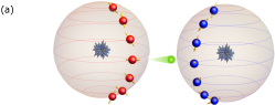
We introduce four-flavor fermions with layer and spin indices living on the fuzzy sphere (see Fig. 1(a)).
Consequently, we consider a real-space Hamiltonian:
where the local density operator of layer- is and the total density is . For simplicity we consider the potentials to be short-ranged interactions , and
, and we set , which are optimized to minimize the finite-size effect. The transverse field strength controls tunneling effect between two different layers.
Figure 1: (a) Sketches of the bilayer fuzzy sphere model: Interacting fermions move on a fuzzy sphere bilayer; and the fermion is able to tunneling between two layers.
(b) A schematic plot of phase diagram with a critical point separating a paramagnet from a symmetry breaking Heisenberg magnet.
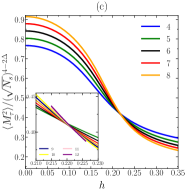
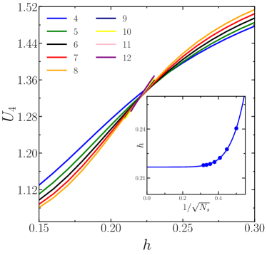
(c) Finite size scaling of order parameter , where is the scaling dimension of the vector field relating to the critical exponent . is the number of Landau orbitals (i.e. Heisenberg spins), which relates to the length scale radius as .
(d) The data collapse of the rescaled order parameter
according to with and , where is a free fitting parameter. The best fit gives . (e) Finite size scaling of crossing points by a finite-size pair gives rise to an extrapolated value .
In practice, we consider the second quantization form of this model by the projecting to the lowest Landau level (see Supple. Mat. Sec. A sm ),
using .
Here the number of Landau orbitals plays the role of system size ( is the radius of sphere). We consider the Landau level is filled by electrons in total.
This model possesses the rotation symmetry of sphere, the global symmetry, the layer inversion symmetry , and the particle-hole symmetry , in addition to the charge conservation.
Numerically, this model is solved using exact diagonalization and density matrix renormalization group (DMRG) White (1992); Feiguin et al. (2008). We perform DMRG calculations with bond dimensions up to , and we explicitly impose three symmetries, i.e., spin-resolved fermion number and -component angular momentum.
For the largest system size , the maximum truncation errors for the ground state is less than .
The phase transition is obtained by the conventional finite-size scaling of the order parameter (i.e. vector), which inspects the spontaneous symmetry breaking
(1)
Utilizing this order parameter, our calculation confirms a direct continuous phase transition from ordered Heisenberg magnet to disordered paramagnet in the proposed model.
At the transition point, the order parameter should scale as Hasenbusch (2023); Sandvik and Scalapino (1994); Wang et al. (2006); Ippoliti et al. (2018),
where is the scaling dimension of vector field Poland et al. (2019a).
Fig. 1 (c) illustrates the rescaled order parameter with respect to the transverse field strength for various .
is almost unchanged near the crossing point , which signals the phase
transition point.
The exact value of critical point can be obtained by two ways: 1) is the best fitting parameter for the data collapse as shown in Fig. 1(d), or 2) through the crossing-point analysis, crossing points for different sizes tend to a extrapolated value , as shown in Fig.1(e).
Importantly, both analysis give a consistent estimation of , which is taken to be the critical point for the following discussion.
Additionally, we have also computed the binder cumulant and the lowest energy gap, finite-size scaling of which confirm the estimation of (see Supple. Mat. Sec. B sm ).
In a word, the critical behavior of order parameter shows
the critical point in this bilayer fuzzy sphere model described by the universality class.
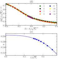
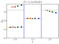
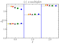
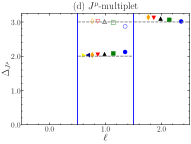
Figure 2: Conformal multiplet of several low-lying primary operators. Scaling dimension versus Lorentz spin for (a) the lowest vector , (b) the lowest rank-2 symmetric traceless tensor , (c) the lowest scalar field and (d) conserved current .
The plots are calibrated by the scaling dimension of the energy-momentum tensor .
Solid (open) symbols represent
parity even (odd) operators.
The dashed horizontal lines are the prediction from conformal bootstrap, and the discrepancy is relatively smaller for the primaries and their first descendants.
Operator spectrum.—
We now turn to the main results of this paper. The great advantage to work on the spherical geometry is, we can unlock the so-called state-operator correspondence Cardy (1984, 1985), i.e. the eigen-energy gap takes the form ,
where is the model-dependent speed of light, and are the scaling dimensions of the CFT operators. Therefore, we compute energy spectra at the critical point and compare it with CFT predictions.
To examine if the eigenstates in this proposed model form representations of 3D conformal symmetry, we analyze the low-lying spectra according to the following rules:
1) We rescale the full spectrum by setting the energy-momentum tensor to be exactly ; 2) The lowest-lying energy states that cannot be generated from other fields are identified as primaries; 3) The descendants are produced by applying raising ladder operators to the identified primary states and by matching the quantum numbers.
For example, for a scalar primary with quantum number (Here is the quantum number of SO rotation symmetry of fuzzy sphere behaving as the Lorentz spin of the conformal group and is the quantum number of global spin rotation symmetry.), its descendants can be written as
, which takes the scaling dimension with quantum number .
Fig. 2 depicts numerically identified conformal multiplet (i.e. primary and its descendants) of the lowest vector , the lowest traceless tensor , the lowest scalar and the Noether current .
Remarkably, we found that the low-lying eigen-states approximately form representations of the 3D conformal symmetry up to small finite-size corrections.
This is a direct and unambiguous demonstration of the emergent conformal symmetry of the 3D Wilson-Fisher transition. To our best knowledge, such direct evidence has not been reported before. Additionally,
the numerical discrepancy is typically more significant for the fields with larger and larger angular momentum , which is attributed to the finite-size effect: The CFT only captures the low-energy effective theory for our model, and to access large angular momentum fields requires the simulation on sphere with large enough radius.
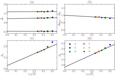
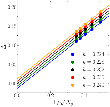
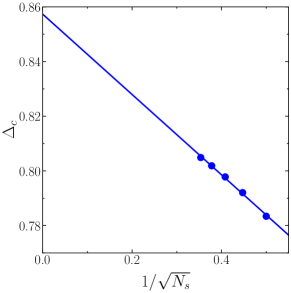
Figure 3: Finite-size extrapolations of the scaling dimensions of (a) the lowest vector , the lowest rank-2 tensor , and the lowest scalar field , (b) gap of descendant field , (c) the lowest rank-3 tensor and (d) the lowest rank-4 tensor . Finite-size extrapolations with system sizes give rise to , , , , , and .
Table 1: Low-lying primary operators identified via state-operator correspondence on the fuzzy sphere. We only take the first three digits from the data in literature. Error analysis see Sec. E. sm .
expHenriksson (2023); Manuel Carmona
et al. (2000)
After verifying the emergent conformal symmetry, we further compare scaling dimensions of the identified primary operators with the existing data from various methods Hasenbusch (2023); Pelissetto and Vicari (2002); Chester et al. (2021); Poland et al. (2019a); Kos et al. (2014); Wang et al. (2006); Kleinert and Schulte-Frohlinde (1995); Guida and Zinn-Justin (1998); Manuel Carmona
et al. (2000).
As listed the relevant primary operators that we have identified in Tab. 1, overall we find a reasonable agreement with numerical bootstrap Poland et al. (2019a); Chester et al. (2021) and Monte Carlo data Hasenbusch (2023), e.g. the averaged discrepancy from the bootstrap data is less than .
Despite of the small discrepancy, the precision is still sufficiently high to further increase the confidence that the universality class of the transition falls into the 3D Wilson-Fisher type.
In particular, these data are crucial to understand the physics of critical point. For instance, the lowest rank-4 symmetric tensor operator corresponds to the anisotropic cubic perturbation. This operator is dangerously relevant, according to the existing numerical computation Chester et al. (2021); Henriksson (2023). Although the finite-size value of its scaling dimension flows (Fig. 3 (d)), our calculation confirms its relevance .
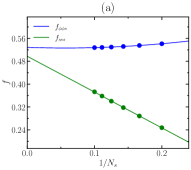
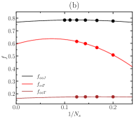
Figure 4: (a) Two representative OPE coefficients involving the scalar primary (blue) and (green).
(b) Three representative OPE coefficients involving the energy-momentum tensor (brown), (red) and the conserved current (black).
The finite-size extrapolation is up to , where data are from the ED and data are from DMRG.
Table 2: List of the OPE coefficients from the fuzzy sphere and comparison with the bootstrap data Poland et al. (2019a); Chester et al. (2021). Error analysis see Sec. E. sm .
Correlation functions and OPE coefficients.—
Besides the state perspective, we can also study the operator perspective of the identified primaries.
Here let us take the OPE coefficient as an example.
Since relates to the local operator , we have Hu et al. (2023)
(2)
(3)
where ’’ denotes the contribution from other primaries and associated descendants.
Thus, we can compute using
(4)
To eliminate the two leading corrections from the descendant fields , we perform a finite-size extrapolation up to (i.e. ). Similarly, other OPE coefficients can be extracted within the same method sm .
To quantify the data of OPE, we compare our results with the numerical bootstrap data Chester et al. (2021); Poland et al. (2019a) in Tab. 2.
The data are in overall agreement.
The ability to access both scaling dimensions and OPE coefficients together shows the superiority of fuzzy sphere scheme.
Summary and discussion.—
We have constructed a microscopic model of Heisenberg magnet bilayer living on the space-time geometry , which realizes a order-disorder transition belong to Wilson-Fisher universality class.
At the phase transition point, clear evidence of emergent conformal symmetry is observed by identifying the one-to-one correspondence between CFT operators and the eigenstates, through which we are able to identify conformal data including the scaling dimensions and OPE coefficients of relevant primary operators. These information are crucial to understand the stability of Wilson-Fisher fixed point under various perturbations.
In addition, the proposed bilayer fuzzy sphere model can also capture the essential physics of three-dimensional XY transition belong to Wilson-Fisher class, by properly adjusting the global symmetry of quantum spins (see Supple. Mat. sm ).
In this context, the current work extends the horizon of the fuzzy sphere scheme to general Wilson-Fisher universality class with continuous global symmetry, which demonstrates the vibrancy of this newly proposed method. We envision the fuzzy sphere will be a powerful tool to explore 3D CFTs in more exotic criticalities.
Acknowledgements.
Acknowledgment.— We thank Yin-Chen He for simulation discussion and collaboration on related projects. We thank Ning Su for useful discussions. This work was supported by National Science Foundation of China under No. 92165102, 11974288.
Note added.— We become aware of another work on XY transition using fuzzy sphere scheme: arXiv.2310.xxxxx.
Polyakov (1970)
A. M. Polyakov,
JETP Lett. 12,
381 (1970).
Philippe Francesco (1997)
D. S. Philippe Francesco,
Pierre Mathieu, Conformal Field
Theory, Graduate Texts in Contemporary Physics
(Springer New York, NY, 1997), ISBN
978-1-4612-2256-9.
Rychkov and Vichi (2009)
V. S. Rychkov and
A. Vichi,
Phys. Rev. D 80,
045006 (2009), eprint 0905.2211.
El-Showk et al. (2012)
S. El-Showk,
M. F. Paulos,
D. Poland,
S. Rychkov,
D. Simmons-Duffin,
and A. Vichi,
Phys. Rev. D 86,
025022 (2012), eprint 1203.6064.
Zhou et al. (2023)
Z. Zhou,
L. Hu,
W. Zhu, and
Y.-C. He,
The deconfined phase transition under
the fuzzy sphere microscope: Approximate conformal symmetry,
pseudo-criticality, and operator spectrum (2023),
eprint 2306.16435.
In this supplementary material, we will show more details to support the discussion in the main text. In Sec. A, we discuss the spherical Landau levels, then derive the second-quantization form of the real-space Hamiltonian and connection to Haldane pseudopotential.
We also explain the intuition of fuzzy sphere bilayer model for general Wilson-Fisher (N) transitions.
In Sec. B, we provide more detailed analysis on the finite-size scaling of physical observables, the binder cumulant and the lowest energy gap, across the phase transition. We also calculate the charge gap to demonstrate that the degree of freedom in the low-energy region is Heisenberg spin. In Sec. C,
we show how to get the OPE coefficients using spin operators and derive the finite-size scaling forms. Meanwhile, we calculate and show the result of two-point correlation function of in Sec. D. In Sec. E, we present the detail of numerical data and error analysis.
.1 A. 1. Spherical Landau levels
We consider a sphere with radial , and a monopole located in the center of the sphere. The Hamiltonian for an electron moving on the surface has only the kinetic term Haldane (1983)
(S1)
where is the electron’s mass and is the covariant angular momentum, is the gauge field of the monopole. Here we have set . Corresponding eigen energies are known as the famous Landau levels, , with the Landau level index. The Landau level has -fold degenerate, and the single particle states in each Landau level are called Landau orbitals.
The wave functions for each Landau orbital on LLL are called monopole harmonics Wu and Yang (1976)
(S2)
Here , the normalization factor , and is the spherical coordinates.
.2 A. 2. Second-quantization Hamiltonian
Here we derive the second-quantization form of the real-space Hamiltonian. Firstly, we define the total density operator as
(S3)
where we have used the monopole harmonics derived above. The angular momentum decomposition of the total density operator is given by
(S4)
Here, . Here labels the layer index and represents the spin index. is the spherical harmonics. And the angular momentum decomposition of the local density operator of layer- is
(S5)
Throughout this paper, the notation and means and .
For any two-body interaction potential depending on on the spherical geometry, it can be expanded in Legendre polynomials
(S6)
Taking the first term in the as an example, we can obtain its second-quantization form is
(S7)
Similar form can be found for the second and third term. Finally, our second quantization form of the real-space Hamiltonian is given by
(S8)
.3 A. 3. Relationship with the Haldane pseudopotential
The real-space interactions we used in the main text are connected to the Haldane pseudopotential . For the cases of potential and its derivative, the only non-zero component of the Haldane pseudopotential is and , respectively. Similarly, we can use the Haldane pseudopotential to reformulate the Hamiltonian
(S9)
and the parameter
is connected to the Haldane pseudopotential by
(S10)
By comparing the coefficients, we can get the relations between and ,
(S11)
Here, is Wigner coefficient.
.4 A.4 Connecting with the models
In the main text, we have shown a microscopic realization of Heisenberg-like model exhibiting Wilson-Fisher transition. Here we discuss that
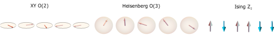
the proposed fuzzy sphere bilayer model has far-reaching extension to realize general universality class of Wilson-Fisher transition with (Ising), (XY) and (Heisenberg).
To clarify the construction, we rewrite the density-density interaction in each layer as (The interlayer interaction doesnot specify here)
(S12)
The definition of local density operators are in line with the main text:
the local density operator of layer- is .
Here setting favors the Heisenberg symmetry as discussed in the main text, which preserves the spin rotation symmetry. We refer as Heisenberg point in the following discussion.
Further tuning the parameter leads to different global symmetry of effective spin degrees of freedom:
1) (“easy-axis” condition) leads to a Ising symmetry;
2) (“easy-plane” condition) leads to a XY symmetry.
Moreover, we should be careful on the form of interactions.
For the Heisenberg model in the main text, we choose short-ranged interactions to be . This form of interaction is special to achieve spin, because potential is always SU(2) symmetric. To realize the XY transition and Ising transition, one also needs to modify the form of density-density interaction. In specific, we use the following form:
(S13)
Tuning the parameters and breaks the spin rotation symmetry and
produce XY spin or spin.
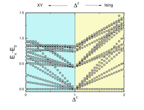
To demonstrate it, we compute the energy spectrum of a single layer model as a function of , in Fig. S1. At the Heisenberg point, the ground state is -fold degenrated guaranteed by the spin rotational symmetry for quantum spins. For , the ground state is doublet degenerated, related to the symmetric breaking Ising spin. For , the ground state belongs to the XY spin order.
Figure S1: (Top panel) Fuzzy sphere model can simulate magnetic order with symmetry: (Ising), (XY) and (Heisenberg).
(Bottom panel) Energy spectra of as a function of . At the Heisenberg point , the ground state is -fold degenerated. By tuning away from the Heisenberg point leads to quantum XY spins or quantum Ising spins.
Based on the magnetic orders with different symmetries established on the fuzzy sphere bilayer model, one can further construct phase transitions belong to Wilson-Fisher (N) universality class: (Ising), (XY) and (Heisenberg). The Ising transition should be in line with the existing discussion Zhu et al. (2023), and the Heisenberg transition has been studied in the main text. We believe that the XY transition can be also realized in the fuzzy sphere bilayer model in a similar way.
Finally, let us make some remarks here. Previously we have realized a 3D Ising transition on the fuzzy sphere model with one-layer Zhu et al. (2023) (We dubbed it as single-layer fuzzy sphere model).
The idea is to use a spin-flip transverse field term (i.e. involving operator) to induce a paramagnetic phase. Unfortunately, this single-layer fuzzy sphere model cannot realize the XY or Heisenberg transition. The reason is, the spin-flip transverse field term involving operator explicitly breaks the spin rotation symmetry, so that a or symmetric paramagnet cannot be created on the single-layer fuzzy sphere model.
Here to overcome this obstacle, we turn to construct a fuzzy sphere bilayer model, which is able to realize the (N) transition with global continuous symmetry. In this context, the fuzzy sphere bilayer model is meaningful, which goes beyond the limitation of single-layer fuzzy sphere model.
Appendix A B. Physical observables across the phase transition
In the main text, the critical point of the phase transition is determined by the scaling of local order parameter.
In this section, we consider two more physical observables, the binder cumulant and the lowest energy gap, and study their finite-size scaling around the phase transition to confirm the estimation of . In the end, we calculate the charge gap to show that spin is the degree of freedom in the low-energy region.
The binder cumulant Hasenbusch (2023) is defined as
(S14)
It is a universal quantity related to the four-point field at the phase transition. Fig. S2 (a) shows with respect to the transverse field strength for different . Clearly, at small the model is the ordered Heisenberg magnet, while at large the model is the disordered paramagnet. There is a crossing region , where different system sizes cross with each other. The precise value of critical point can be determine by the crossing-point analysis according to the scaling form , shown in Fig. S2 (a) (inset).
This is the same analysis as how we used the order parameter in the main text, while the critical point is a little smaller.
Secondly, we compute the energy gap between the ground state and the first excited state for different system sizes , and do finite-size scaling. As one can find in Fig. S2 (b), below , the energy gap is smaller than , while it becomes gapped when exceeds , which gives rise to . Three different physical observables, including the order parameter in the main text, are largely consistent with each other.
Figure S2: The binder cumulant with different system sizes . (Inset) Finite-size scaling of crossing points by a finite-size pair , which gives rise to . The scaling form is .
Figure S3:
(b) Finite-size scaling of the lowest energy gap with different for various , which gives us the critical point .
Thirdly, the original fuzzy sphere model consists of fermionic degrees of freedom. So one preliminary question to be addressed in the model design is whether or not the charge excitation gap is relevant to the discussion of magnetic phase transition. Here we define the charge gap as , where is the ground state energy on lowest Landau level orbitals filled by electrons. After obtaining the charge gap on each system size, we perform a finite-size scaling to estimate the charge gap in the thermodynamic limit. As shown in Fig. S4, the charge gap at the critical point is nonzero on all system sizes, and the value in the thermodynamic limit is also finite. Thus, we conclude that the spin degrees of freedom undergoes a phase transition while the charge degrees of freedom are always gapped. And close to the phase transition point the spin excitation, rather than the charge excitation, dominates the low-energy excitation.
Figure S4: Finite-size scaling of charge excitation gap with system sizes at the phase transition point .
Appendix B C. OPE coefficients
This section delves into the nuances of calculating OPE coefficients, emphasizing the tensor structures and accounting for finite-size corrections.
B.1 C.1. Tensor structures
In our main text, we have analyzed five OPE coefficients, namely and . These coefficients correspond to four primary fields: , , , and . Here, we outline their tensor structures:
(S15)
Where serves as the auxiliary coordinate, devoid of indices, pertinent to the Lorentz tensor. The indices , , and relate to the global structure. Within the OPE linked to the current operator, the tensor functions as the generators. It’s crucial to recognize that the tensor structures of these OPEs use the two-point correlators for normalization.
(S16)
Here, denotes the unit vector and . To recover the explicit indices, one can apply the differential operator relative to the auxiliary coordinate :
(S17)
The operator, exhibiting explicit Lorentz quantum numbers , alongside quantum numbers , , can be formulated as:
(S18)
where and are Lorentz and polarization respectively. By leveraging the state-operator correspondence, this operator transforms into the state within the numerical states, subject to normalization
(S19)
Thus
(S20)
where comes from the conjugation.
For a deeper insight, let’s examine the tensor structure of the OPE as a representative example. For comprehensive tensor structures associated with other OPEs, readers are directed to earlier worksHu et al. (2023); Zhou et al. (2023).
The correlators related to and are
(S21)
Both the Lorentz and polarizations serve as spherical tensors for the rotation group. Therefore:
(S22)
Consequently, the normalization factors for and are:
(S23)
Following the same procedure, the OPE of in is:
(S24)
By integrating the angle dependence and taking into account the angular momentum component
(S25)
and the factor can be offset by its two-point correlator
(S26)
In conclusion, the value of is:
(S27)
Now we discuss about other OPEs. Since they are both scalar-scalar-scalar(spin- tensor) type, we can directly use the results in Ref.Hu et al. (2023); Zhou et al. (2023) after treating the scalar in the vector representation of . If we choose the component of , the polarization is just and will not produce any modification. Finally, we have
(S28)
B.2 C.2. Relation to central charge
The relation between OPE coefficients and the central charge is evident from the study of their correlators. Specifically, the OPE coefficients, denoted by and , can be associated with the central charge and the current central charge . These relationships are determined by the correlators:
(S29)
By referencing Ref.Poland et al. (2019b), we find the CB prediction values of the central charge:
(S30)
These approximations utilize bootstrap values from Ref.Chester et al. (2021); Poland et al. (2019b), where and . Additionally, theoretical values cited from Ref.Petkou (1995) provide and .
B.3 C.3. Finite size corrections
In this section, we will provide a thorough finite-size scaling of OPE coefficients Hu et al. (2023) from the microscopic spin operators.
Since the lowest vector corresponds to the local order parameter, and the lowest scalar in the Wilson-Fisher description using quantum field theory. We will choose local operator to approach the CFT operator , and to approach . The operator decomposition generically is,
(S31)
where the first four terms represents the primary and components of its descendants. More other descendants of , and other primaries and corresponding descendants, included in . Similarly, the operator can be disassembled by
(S32)
Two scaling dimensions are and , respectively. Now, we can extract the OPE coefficient by ,
for which only operators with same quantum number will contribute,
(S33)
Similarly, can also be computed by
(S34)
and the finite-size scaling of the OPE coefficient reads
(S35)
The OPE coefficients involving spinning operator are slightly more complicated, since one has to carefully deal with the dependence. We compute . The finite-size scaling of the OPE coefficient is given by
(S36)
Similarly, and can be computed by
(S37)
and
(S38)
respectively.
Appendix C D. Two-point correlator
In this section, we would like to study the correlator on the fuzzy sphere. We will use the operator as an example.
The decomposition of local operator is following Eq. S31.
The normalized two-point function of receives its leading order contribution from the two-point function of :
(S39)
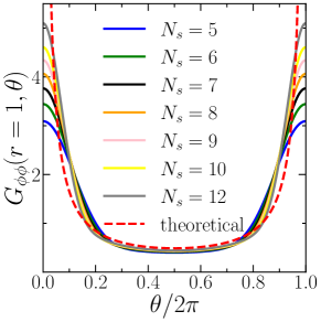
Fig. S5 depicts the two-point correlator by setting as a function of . In this case, is a dimensionless function that solely depends on the angle between the two operator. Overall, the finite-size results approach theoretical expectation as increases. The discrepancy is relatively large at small angle. For (close to equator), the different curves almost merge together.
Figure S5: The angle dependence of the two-point correlator is plotted for system sizes .
Appendix D E. Details of numerical data
D.1 E.1 Raw numerical data
Table S1: Scaling dimensions of fields in model (). The data from the fuzzy sphere model (FS) are rescaled by setting . Here data are from the ED and data are from the DMRG.
spin ()
charge ()
Operator
Dimension (CB)
Dimension (FS) ()
Dimension (FS) ()
0
1
0.519
0.521
0.522
0
2
1.210
1.244
1.243
1
1
1.519
1.496
1.498
0
0
1.595
1.595
1.597
1
1
2
2.038
2.032
0
3
2.038
2.150
2.145
1
2
2.210
2.256
2.258
2
1
2.519
2.504
2.529
0
1
2.519
2.609
2.604
1
0
2.595
2.643
-
0
4
2.99
3.229
3.216
2
0
3
3
3
2
1
3
3.138
-
1
1
3
3.018
-
In this section, we present the data of energy spectra and corresponding conformal multiplet of various fields in Tab. S1. Here we only present the data for relevant fields ().
Importantly, we emphasize that, the operator spectrum doesnot miss any CFT field or contain any extra non-CFT state in the regime ().
These data are used for plotting the figures in the main text.
For comparison, we also list the results from conformal boostrap method Chester et al. (2021); Poland et al. (2019a).
These detailed data gives a good quantification for the numerical error. That is, scaling dimensions of the low-lying fields are quite close to the results of conformal bootstrap, and the trend towards thermodynamic limit is correct for most of fields.
A rigorous error analysis based on the finite size scaling will be presented in the next subsection.
Another interesting point is that, almost perfect state-operator
correspondence is manifest in surprisingly small system sizes, e.g. the numerical data at a given system size , which is the largest system size that we can reach using ED, is already close to the 3D CFT data. Here, to further elucidate that the numerical findings indeed reflect the physics in the thermodynamic limit, we show the energy spectra on different system sizes.
As one can see that, the energies on different system sizes match the prediction of 3D CFT quite well.
A part of data can be accessed in the DMRG computation.
In the DMRG calculation, we explicitly implement three U(1) symmetries, i.e. z-component angular momentum quantum number , total electron number , and z-component spin .
Making use of the symmetry information of the different fields, we can simplify the DMRG calculation. For example, to target the lowest (3) vector field , we can calculate the lowest energy state in the sector (instead of directly targeting higher excited states in ). Accessing the ground state in different symmetry sectors usually gets fast convergence compared with targeting the excited states.
For the DMRG calculations, we only focus on the low-lying fields, so some of data are missing in Tab. S1 (last column).
D.2 E.2 Error analysis
At last, we present an error analysis of obtained scaling dimensions. Generally, the typical length scale , the radius of fuzzy sphere, should be scaled with the number of Landau orbitals (i.e. spins) as . behaves as the typical length scale as in the flat spacetime lattice model. To extrapolate the numerical data to the thermodynamic limit , we use the polynomial function
, and fit the finite-size data using least-square method. The mean values give the best estimate of the scaling dimensions in the thermodynamic limit, and the residual give the relative errors (See Tab. S2).
Table S2: Extrapolated scaling dimensions of low-lying primary operators identified via state-operator correspondence on the fuzzy sphere.
Fuzzy sphere
0.5240.004
1.2110.008
1.5880.009
2.0280.011
2.9610.012
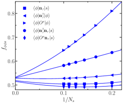
Next, we further analyze the error of obtained OPE coefficients. The strategy used to estimate errors are explained below. Following the discussion in Ref. Hu et al. (2023), we utilize the different local operators to estimate the OPE coefficients. (The general idea is Zou et al. (2020), the information of CFT primary field may be encoded in different local operators, and it is expected different local operators should give the same OPE coefficients since the OPE coefficients should be universal.)
First of all, we need to analyze the operator content of different local operators based on the symmetries. In short, the following local operators have significant weights with the primary fields :
(S40)
(S41)
(S42)
(S43)
(S44)
Using the local operators listed above, we can estimate the OPE coefficients. For example, when estimating the OPE coefficient , one could use two different ways to calculate it: 1) (see Eq. S33) by using the local operator , , or and 2) (see Eq. S34) by using the local operator or .
Fig. S6 shows the five different estimations. By extrapolation, the estimated values of are 0.518 from , 0.529 from , 0.532 from , 0.530 from , and 0.515 from . So the mean value and relative error are estimated to be
(S45)
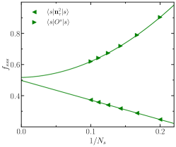
Similarly, the estimated values of are 0.498 from and 0.517 from (see Fig. S6). So the mean value and relative error are given by
(S46)
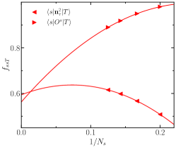
Meanwhile, the estimated values of are 0.594 from and 0.563 from (see Fig. S6). Their mean value and relative error are given by
(S47)
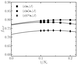
The estimated values of are 0.768 from , 0.772 from , and 0.715 from (see Fig. S6). Their mean value and relative error are given by
(S48)
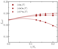
The estimated values of are 0.164 from , 0.164 , and 0.163 from (see Fig. S6). Their mean value and relative error are given by
(S49)
We find the estimates of from three different local operators are quite close to each other, so the relative error is much smaller.
At last, we need to emphasize, although the above errors are not rigorous, we think this is the best way to do the error analysis Hu et al. (2023). That is, compared with the error in the fitting process, the relative errors from the fitting using different local operators are relative larger. So we would like to use this way to estimate the error of OPE coefficients.
Table S3: Extrapolated OPE coefficients of low-lying primary operators identified via state-operator correspondence on the fuzzy sphere.
Fuzzy sphere
0.5250.007
0.5070.010
0.5780.016
0.7520.025
0.16850.0003
Figure S6: (Top left)
Finite-size scaling of five different quantities to estimate the OPE coefficient .
(Top middle)
The OPE coefficient can be estimated by two different local operators and .
(Top right) The OPE coefficient can be estimated by two different local operators and .
(Bottom left)
Finite-size scaling of three different quantities to estimate the OPE coefficient .
(Bottom right) The OPE coefficient can be estimated by two different local operators and .