Exposing Disparities in Flood Adaptation for Equitable Future Interventions

Abstract

As governments race to implement new climate adaptation policies that prepare for more frequent flooding, they must seek policies that are effective for all communities and uphold climate justice. This requires evaluating policies not only on their overall effectiveness but also on whether their benefits are felt across all communities. We illustrate the importance of considering such disparities for flood adaptation using the FEMA National Flood Insurance Program Community Rating System and its dataset of $\sim$2.5 million flood insurance claims. We use CausalFlow, a causal inference method based on deep generative models, to estimate the treatment effect of flood adaptation interventions based on a community’s income, diversity, population, flood risk, educational attainment, and precipitation. We find that the program saves communities $5,000–15,000 per household. However, these savings are not evenly spread across communities. For example, for low-income communities savings sharply decline as flood-risk increases in contrast to their high-income counterparts with all else equal. Even among low-income communities, there is a gap in savings between predominantly white and non-white communities: savings of predominantly white communities can be higher by more than $6000 per household. As communities worldwide ramp up efforts to reduce losses inflicted by floods, simply prescribing a series flood adaptation measures is not enough. Programs must provide communities with the necessary technical and economic support to compensate for historical patterns of disenfranchisement, racism, and inequality. Future flood adaptation efforts should go beyond reducing losses overall and aim to close existing gaps to equitably support communities in the race for climate adaptation.

1 Introduction

Flooding constitutes nearly a third of all losses from natural disasters worldwide (Reuters, 2022). In the US alone, flooding causes more damage than any other severe weather-related event, with annual losses averaging over $5 billion (NOAA, 2014). These losses are only expected to multiply as climate change raises the sea level and increases the frequency of extreme weather events (Rodell & Li, 2023). By the end of the century, rising sea levels and coastal flooding are estimated to cost the global economy $14.2 trillion (a fifth of the global GDP) in damaged assets (Kirezci et al., 2020). In response, communities are rapidly enacting flood adaptation measures (Jongman et al., 2014; Wahl et al., 2015; Alfieri et al., 2016). As these measures have emerged so has evidence of their success (Deegan, 2007; Highfield & Brody, 2017; Asche, 2013; Brody et al., 2009; Davlasheridze et al., 2013; Kousky & Michel-Kerjan, 2017). However, there is still a gap in understanding whether and how the effectiveness varies across different communities.

A better understanding of the effectiveness of flood adaptation policies and their connections to the communities implementing them can ensure that they have the intended effect. It can also ensure that flood adaptation investments deliver on the desired goals and effectively allocate limited resources for climate adaptation. Furthermore, it can prevent climate interventions from unknowingly replicating historical patterns of discrimination (Mitchell et al., 2015; Simpson et al., 2022; Ranganathan & Bratman, 2021). This is especially critical in light of recent evidence highlighting patterns of inequality in flood preparedness and recovery processes in the US (Cutter & Finch, 2008; Emrich et al., 2020; Tate et al., 2021; Wing et al., 2022; Flores et al., 2023).

We reexamine the effectiveness of flood adaptation interventions by evaluating not only whether they are effective but also for whom. We measure the effectiveness of flood adaption interventions across different types of communities using a US wide data set on flood insurance payments from the National Flood Insurance Program (NFIP) Community Rating System (CRS). FEMA initiated the CRS in 1990 in order to improve community flood adaptation and resilience. The program is based on a set of prescriptive activities recognized as best practices for flood risk reduction. These constitute flood adaptation recommendations that are prevalent in flood planning across the world. To join the CRS, communities must implement a series of flood adaptation activities: e.g. floodplain mapping, open space preservation, stormwater management activities, or public information and participation programs. In exchange, residents of the community receive a discount on their flood insurance premium rates. More than 1,500 out of roughly 20,000 communities in the NFIP are currently part of the CRS program (FEMA, 2021).

In 2019, FEMA released the NFIP Redacted Claims data set that contains roughly 2.5 million flood insurance claims. It contains claims from communities participating in the CRS as well as claims from communities who did not participate in the CRS, but were eligible for insurance coverage because they complied with minimum floodplain regulation requirements. Thus, the Redacted Claims data set provides an ideal quasi-experimental setup. Insurance claims losses, which we use as a proxy for flood loss, can be compared between CRS participants and non-participants to quantitatively assess the effectiveness of the CRS flood adaptation activities.

Capitalizing on this quasi-experimental setup, past literature examined whether the CRS led to a reduction in flood claims (Michel-Kerjan & Kousky, 2010; Davlasheridze et al., 2013; Highfield & Brody, 2017; Kousky & Michel-Kerjan, 2017; Gourevitch & Pinter, 2023). Despite some studies finding the contrary (Asche, 2013), the overall consensus is that flood losses are reduced by the CRS. There has been, however, little investigation on whether the program’s effectiveness varies across different types of communities. There has also not been any systematic analysis on the disparities in flood adaptation initiatives across communities in the broader international literature.

Past literature has shown that low-income communities respond to risks differently to safeguard their livelihoods (Haque, 2021) and deploy flood-coping mechanisms in the absence of flood protection (Brouwer et al., 2007). It also highlighted the need to promote pro-poor climate adaptation initiatives and acknowledge the need need to strengthen low-income household’s asset base to improve their adaptation (Mearns & Norton, 2010). Furthermore, some studies have predicted flood losses and vulnerabilities for different types of communities (Knighton et al., 2020; Wing et al., 2020; Yang et al., 2022). Nevertheless, no work so far quantifies how the benefits/savings of flood adaptation activities are distributed across different communities. That is the main goal of this paper.

Accurately estimating the causal effect of flood adaptation policies and its dependence on community characteristics requires modeling their relationship. This is especially challenging since the relationship can be highly non-linear, complex, and correlated, which violates the assumptions of many standard causal inference methods. In this work, we tackle these challenges using CausalFlow, a novel method that leverages deep generative models to measure the causal effect in a data-driven approach. With our method, we examine for the first time the effectiveness of the CRS as a function of key community characteristics such as population, income, diversity, and educational attainment at high-resolution on a zip code level over the entire continental US. We conclusively assess the effectiveness of the CRS flood adaptation activities and shed light on who benefits the most from it and under which circumstances. Our results provide key insight for communities tailoring flood adaptation interventions. It also provides a path forward to re-envisioning flood adaptation in ways that can benefit a broader spectrum of communities in the face of climate change.

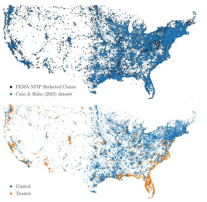
Figure 1: Top panel: We compile our dataset (blue) from the FEMA FIMA NFIP Redacted Claims dataset (black) with additional information on community geo-demographic characteristics (precipitation, flood risk, income, population, renter fraction, educational attainment, and diversity fraction) from additional datasets (Section 2). Bottom panel: Communities that participated in the CRS are part of the treated group (orange), while the communities that did not are part of control group (blue)

2 Data

For this work, we compile a dataset based on the FEMA Flood Insurance Mitigation Administration NFIP Redacted Claims data with additional information on community characteristics. From the NFIP dataset, we use data on CRS participation, the date of flood loss, and the total claims paid on building damages and content from the loss. We combine all the entries for a zip code and calculate the total claims paid per policy.

For each zip code, which we refer to as a community, we quantify its flood risk using scores compiled in the First Street Foundation dataset. The risk scores are computed based on factors including risk of flooding from high-intensity rainfall, overflowing rivers and streams, high tides, and coastal storm surges. We further supplement the dataset with census data from the US Census Bureau American Community Survey, which is compiled in four year intervals: $2008-2012$, $2012-2016$, and $2016-2020$. We assign median income and number of residents (population) of the communities based on their zip code and date of loss. We also calculate the fraction of residents that rent, have a Bachelor’s degree or more advanced degrees, and do not identify as only white. We refer to each of the characteristics as the renter fraction, educational attainment, and diversity fraction, respectively. Lastly, we include average precipitation in millimeters during the month of the flood event for each community. This data was extracted by splitting the PRISM climate group data compiled by the Northwest Alliance for Computational Science and Engineering using US zip code boundaries from 2020.

In total, our dataset includes 14,729 unique communities. In the top panel of Figure 1, we mark the communities that are included in our dataset (blue) from the full NFIP dataset (black) on a map of the US. Our final dataset is publicly available at XXXXX.

3 Methods: CausalFlow

One of the main goals of causal inference is to measure the treatment effect of a policy, like the CRS. For heterogeneous treatments, the effect is quantified using the conditional average treatment effect (CATE), the ATE as a function of covariates. By revealing the dependence of the treatment effect on covariates, CATE provides a more detailed understanding of the causal path. Given outcome $Y$, covariates $X$, and variable $T$ that indicates the control ($T=0$) or treated ($T=1$) groups, CATE is estimated as:

$${\rm CATE}=E[~{}Y\,|\,X,T=1~{}]-E[~{}Y\,|\,X,T=0~{}].$$ (1)

$E[~{}Y\,|\,X,T=0,1~{}]$ represents the expected value of $Y$ given $X$ for the control and treated groups, respectively.

Typically, CATE is estimated using either matching or linear regression. In matching, samples in the treated group are matched to ones in the control based on their $X$ values. CATE is then estimated by comparing the outcomes of the matched samples. Even prevalent methods, such as synthetic control (Abadie & Gardeazabal, 2003; Abadie et al., 2010) or propensity score matching (Rosenbaum & Rubin, 1983), match samples based on some finite volume in covariate space, which can lead to incorrect estimates of the CATE.

The other approach is regression, most commonly with linear models (Angrist, 1990; Miguel & Kremer, 2004). A model of $Y$ as a linear function of $X$ is fit to the data and then used to estimate CATE. In many scenarios, assuming a linear model is incorrect. For instance, there is no reason to expect flood losses to depend linearly on its population, or median household income. Furthermore, there is often no a priori knowledge of the functional form that should be adopted for a model of $Y$.

We can instead estimate the CATE without any of these assumptions. We rewrite Eq. 1 as

$${\rm CATE}=\int Yp(Y|X,T=1)\,{\rm d}Y-\int Yp(Y|X,T=0)\,{\rm d}Y,$$ (2)

where $p(Y|X,T=1)$ and $p(Y|X,T=0)$ are the conditional probability distribution of $Y$ given $X$ for the treated and control groups. If we can estimate $p(Y|X,T=1)\approx q_{T}(Y|X)$ and $p(Y|X,T=0)\approx q_{C}(Y|X)$ and sample from them, $Y_{T,i}^{\prime}\sim q_{T}(Y|X)~{}{\rm and}~{}Y_{C,j}^{\prime}\sim q_{C}(Y|X)$, we can estimate CATE using Monte Carlo integration:

$${\rm CATE}=\frac{1}{N_{T}}\sum\limits_{i=1}^{N_{T}}Y_{T,i}^{\prime}-\frac{1}{N_{C}}\sum\limits_{j=1}^{N_{C}}Y_{C,j}^{\prime}.$$ (3)

Deep generative models from machine learning (e.g. ChatGPT, Dall-E) enable us to accurately estimate and sample from $p(Y|X,T=0,1)$. In this work, we use normalizing flow models (Tabak & Vanden-Eijnden, 2010; Tabak & Turner, 2013), which use a bijective transformation, $f:z\mapsto x$, that maps a complex target distribution, $p(x)$, to a simple base distribution, $\pi(z)$, in our case a Gaussian. $f$ is defined to be invertible and to have a tractable Jacobian so that target distribution can be evaluated from the base distribution: $p(x)=\pi(z)|\det\frac{\partial f}{\partial x}^{-1}|$. A neural network is used for $f$ to provide an extremely flexible mapping that can estimate complex distributions. This neural density estimation approach has been used extensively in a variety of fields spanning neuroscience (e.g. Gonçalves et al., 2020) to astrophysics (e.g. Alsing et al., 2019; Hahn & Melchior, 2022).

Using normalizing flows, we estimate $p(Y|X,T=1)\approx q_{\rm T}(Y\,|\,X)$ and $p(Y|X,T=0)\approx q_{\rm C}(Y|X)$ for the treated and control groups separately. We describe the training of our normalizing flows $q_{\rm T}$ and $q_{\rm C}$ in Appendix A. Our outcome, $Y$, is the total insurance claims per policy in dollars. We use seven covariates, $X$: precipitation, flood risk, income, population, renter fraction, educational attainment, and diversity fraction (Section 2). The treated group consists of communities participating in the CRS, while the control group consists of non-participants. In the bottom panel of Figure 1, we mark the communities in the treated (orange) and control (blue) groups of our dataset.

Once trained, we can evaluate CATE at any given value of the covariates using $q_{\rm T}$, $q_{\rm C}$, and Eq. 3, as long as it is within the support of the covariates in our data. We detail how we ensure this in Appendix B. CausalFlow relaxes the strong assumptions made in standard causal inference methods. It learns the detailed relationship between $X$ and $Y$ from the data to provide an accurate and robust estimate of the treatment effect.

Lastly, we introduce a correction, $\Delta Y$, to the CATE to account for the outreach component of the CRS program:

$${\rm CATE}^{\prime}={\rm CATE}+\Delta Y.$$ (4)

Communities in the treated group are informed of how to successfully file their claims. We estimate in Appendix C that the outreach component alone increases the total insurance claims per policy by $\Delta Y\sim$ $9,780. Since this increase is not a reflection of any change in flood losses, the CATE in Eq. 3 underestimates the impact of the CRS. Thus, we include $\Delta Y$ and correct for the effect of outreach to more accurately quantify the treatment effect on flood loss. Throughout this work, we refer to ${\rm CATE}^{\prime}$ as the CRS savings.

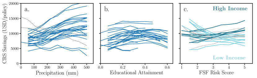
Figure 2: Flood loss savings from the CRS program (CATE’) for 27 community typologies with different population, income, and diversity. In each panel, we vary a single community characteristic, (a) average monthly precipitation, (b) educational attainment, and (c) flood risk score, to highlight its impact on CRS savings. All other characteristics are fixed to fiducial values (Appendix D). The CRS saves policyholders an average of $5,000–15,000 per policy. However, the efficacy of flood adaption depends significantly on income, population, diversity, precipitation, educational attainment, and flood risk.

4 Results

4.1 The Effectiveness of Flood Adaptation Measures

With CausalFlow, we can estimate the impact of the CRS flood adaptation activities on the total insurance claims per policy for any set of community (zip code) characteristics. In other words, we can measure the “treatment effect” of implementing CRS activities and quantify how much a policyholder saves on average thanks to the program. In order to systematize our results, we define 27 distinct community typologies categorized by population, income, and diversity (see Appendix D for details). Then, we compute their CATE’ for different values of average precipitation, flood risk, renter fraction, and educational attainment.

In Figure 2, we present the CATE’ of all 27 community typologies as a function of (a) average precipitation, (b) educational attainment, and (c) FSF flood risk score. In each panel, we vary a single characteristic while keeping all others fixed. We do this for each typology, represented by a single line. This enables us to isolate and examine the effect of a specific characteristic on the CATE’. Overall, we find that the CRS saves policyholders an average of $5,000 - 15,000 per policy. For certain communities, the savings can exceed $20,000. Our findings are consistent with previous evidence, which found that the CRS led to a 40 percent reduction in losses at the county level (Highfield & Brody, 2017) and a $2.8 – 5.5 million reduction in damages for a particular flood event (Michel-Kerjan & Kousky, 2010).

Beyond estimating the overall savings on flood losses, we can also assess the CRS by examining the effect of average precipitation on savings. Flood losses are typically worsened by compounded water runoff from higher precipitation (e.g. Bevacqua et al., 2019; Jang & Chang, 2022; Xu et al., 2023). Yet in Figure 2a, we find that for nearly all of the community typologies, the CRS savings increase with higher average precipitation. Our results firmly illustrate the CRS program’s overall effectiveness in mitigating flood losses.

The program’s overall success does not paint the full story. Our results show that while the CRS is effective, the benefits are not felt evenly across different communities. This serves as critical evidence for rethinking and reimagining future flood adaaptation policies that aim to equitably reduce flood losses for all communities. In the following, we present two lines of action in designing and evaluating future strategies.

4.2 Tailored Requirements and Resources

Community characteristics play a major role in the effectiveness of current flood adaptation measures. To increase flood savings for all communities will require tailoring such measures. For example, while the CRS is effective at reducing flood losses at higher precipitation, certain communities go against this trend. In particular, communities with high population, high diversity, and mid to high income (black dotted in Figure 2a), see their savings steeply decrease with higher precipitation — i.e. flood adaptation measures are less effective. A geospatial analysis of these communities indicates that nearly all of them are in urban areas (Figure 7, Appendix E). Urbanized areas have higher percentages of impervious surfaces that increase water runoff and can cause or worsen flooding (Pasquier et al., 2022). For these urban communities, flood adaptation programs should require activities geared towards e.g. decreasing surface imperviousness.

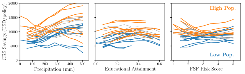
Figure 3: The population dependence on the CRS savings. We present the CRS savings for the 27 community typologies, same as in Figure 2, highlighting the high population (orange) and low population (blue) communities. Flood adaptation measures are more effective for high population communities, who save $\sim$$4000 per policy more than low population communities.

We also find a significant population dependence. In Figure 3, we present the CRS savings for the 27 community typologies as a function of precipitation, flood risk score, and educational attainment, same as in Figure 2. We highlight the communities with a high population in orange and a low population in blue. Overall, flood adaptation measures are more effective for high population communities. They save $\sim$$4000 per policy more than less populated communities. Combined with previous work, which found that highly populated communities are also more likely to adopt CRS activities (Asche, 2013), our results suggest that flood adaptation programs favor populous communities.

Less populated communities may not have the personpower required to implement the prescribed activities, e.g. lacking access to public servants and workers with a wide range of technical expertise. The smaller tax base may also limit the resources available to implement flood adaptation. In field interviews, we found that the acquisition or relocation of flood-prone buildings was limited by the lack of resources available at the local level. The implementation of some CRS activities may also require the types of public services or resources that are not economically feasible for small communities. For instance, the implementation of a flood mapping exercise may prove resource intensive. Hence, future programs should provide the necessary technical support and incentivize collaboration among adjacent communities.

Finally, we find that the effectiveness of the CRS depends on the communities’ educational attainment. In Figure 2b, we present the CRS savings for the 27 community typologies as a function of educational attainment, which we define as the fraction of inhabitants with a Bachelor’s or higher degree. Past evidence already suggests that there is an initial barrier to joining the CRS related to education, where communities with higher educational attainment are more likely to participate (Posey, 2008; Li, 2012; Fan & Davlasheridze, 2014). Our results show that even after communities join, the effectiveness hinges on their education. The dependence on education translates into a gap of up to $\sim$$2,000 per policy in savings.

Out of the 19 creditable activities that communities can implement, many require significant capacity building and technical expertise: e.g. the establishment of flood warning systems and the building and inspection of levees. Communities with lower educational attainment may not have the expertise readily available and community buy-in may be more difficult. In response, future programs should include interventions that reduce the educational/technical barriers and provide the necessary technical assistance along with tailored community outreach resources.

The trends presented in this section make it clear that future flood adaptation programs should tailor their required adaptation measures. This is especially the case if program implementation is linked to incentives such as flood insurance price reduction. If programs reward a community’s adaptation, then not all “low hanging fruit” interventions should qualify for the reward. Instead, communities should be required to implement the types of flood adaptation interventions that are most effective for their needs. At the same time, future programs must furnish communities with the necessary resources to overcome any financial/technical/educational barriers in complying with such requirements. Only then we can expect a just and equitable distribution of the benefits of climate adaptation. Next, we illustrate the importance of considering the inequities and disparities of flood adaptation programs.

4.3 Climate Justice

An effective and far-reaching flood adaptation strategy requires embedding climate justice at its core. Our results show that the effectiveness of a program is tied to economic and racial disparities. For example, although flood adaptation is effective overall for low-income communities, it is less effective when they are located in high flood risk zones. The trend is reversed for affluent communities. We highlight this in Figure 2c, where we show CRS savings as a function of flood risk for low (light blue) and high-income (dark blue) communities. Our results suggests that the most economical CRS activities may only be effective at lower risk. Meanwhile interventions that fare well at higher risk can only be afforded by high-income communities. Evidently, flood adaptation cannot be left to a community’s resources alone, especially since average annual flood losses are disproportionately borne by poorer communities (Wing et al., 2022).

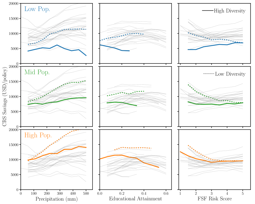
Figure 4: CRS savings for low-income communities with high (solid) and low diversity (dotted; predominantly white) as a function of precipitation (left), educational attainment (center), and flood risk (right). We include the other community typologies for reference (gray). Although both communities have the same income level, highly diverse communities have significantly lower flood loss savings. The gap between high and low diversity exists for communities with low (blue; top), mid (green; middle), and high (orange; bottom) populations. This diversity gap exceeds $6,000 per policy in certain cases.

Furthermore, we find that even within low-income communities, there is a systematic gap in the CRS savings between diverse and predominantly white (low diversity) communities. In Figure 4, we present the CRS savings for low-income communities with high (solid; predominantly white) and low diversity (dotted; predominantly non-white). Since the highlighted communities have the same low income, the comparison between the solid and dotted lines illustrates the sole effect of diversity. Overall, the program is significantly less effective for communities with higher diversity. In some cases, the gap exceeds $6,000 per policy. This points to the program’s inability to breach existing patterns of discrimination and racial inequality (Mitchell et al., 2015; Ranganathan & Bratman, 2021; Simpson et al., 2022).

This gap is consistent with patterns of inequality found in flood preparedness and recovery more broadly (Cutter & Finch, 2008; Emrich et al., 2020; Tate et al., 2021; Wing et al., 2022). Flores et al. (2023) exposed inequalities in the delineation of flood zones in FEMA maps, where “Black and Asian neighborhoods experience disproportionate risk in federally overlooked pluvial and fluvial flood zones” (p.1). Other works have shown that the type of flood adaptation measures employed correlate with diversity (Siders & Keenan, 2020). Measures like “retreat” correlate with high racial diversity while measures like “shoreline armoring” correlate with a less diverse population. Such differences reflect the real choices that historically disenfranchised communities make based on the accessibility of certain types of solutions.

We show that flood adaptation programs can perpetuate institutional racism, through tangible effects on savings, or lack thereof. Future programs should re-examine the processes, structures, and existing assumptions of flood adaptation prescriptions and incentives under the lens of equity, diversity, and inclusion. This will be particularly salient as the evidence overwhelmingly shows that the currently most disadvantaged communities are projected to suffer the most from the consequences of climate change. Embedding these priorities at the core of future programs will be crucial to close existing gaps and support all communities in mitigating flood losses.

5 Discussion & Conclusion

In this work, we find clear trends between flood loss savings and community characteristics. This provides strong evidence that the success of future flood adaptation interventions should not only be measured based on whether they reduce losses, but also on whether the benefits are equitably distributed. Below, we discuss some of the caveats and limitations of our work and outline future research.

First, we note that our results are measured using data from households with access to flood insurance. Hence, our results do not reflect the communities without flood insurance. Even though the threshold to access it is relatively low, it is not negligible. While some of the communities without insurance are ones that face no significant flood risks, they disproportionately include communities without access. Kousky et al. (2020) found that income of policyholders was higher than non-policyholders, which suggests that affordability is a significant concern. In fact, while a quarter of policyholders are classified as lower income, the fraction is over a half for non-policyholders (FEMA, 2018). Although we cannot quantify flood losses for uninsured communities using our dataset, we expect that including their losses would only widen the gaps in savings between privileged and disenfranchised communities.

We also note that the savings estimates in this work are conservative. In calculating the CRS savings, we correct for the outreach component, where communities receive information on how to successfully file their claims ($\Delta Y$ in Eq. 4). This correction is estimated by comparing non-CRS communities to CRS communities that participated in activities for public information and scored below 10% on all other activities. The ideal comparison would be to compare non-participants to CRS communities that only participated in public information activities. However, this includes very few communities, so we relax this selection. This likely leads to an underestimate of $\Delta Y$ and, thus, the CRS savings. Furthermore, our control group consists of communities that did not participate in the CRS but have access to the NFIP, which requires them to regulate floodplain development. Although the requirements are minimal, they may already have a slight effect in reducing losses, which would also make our savings estimate conservative. In subsequent work, we will explore the impact of the outreach component in further detail by examining the proportion of successful payments before and after the implementation of the CRS. Along these lines, we also find signs that the outreach component could be driving elite capture. Savings on flood losses decline for communities with the highest levels of educational attainment (>50%; Figure 2c). Field interviews support the possibility that some households are learning to “game the system” in order to refurbish their homes after a flooding event. Further research, however, is necessary for a more systematic understanding.

Our estimate of flood loss savings is also conservative because preventing damage to homes mitigates further ripple effects in the livelihoods and well-being of communities. Exposure to flood-damaged homes is linked to an increase in mental and health disorders (Graham et al., 2019), death and injury risk, disease outbreaks (e.g. gastroenteritis; Alderman et al., 2012), trauma, anxiety (Walker-Springett et al., 2017), and work disruption (Peek-Asa et al., 2012). For every dollar saved in flood losses in our results, we can expect a far larger reduction in the true loss.

This study underscores the importance of accounting for complex dependencies when evaluating the effectiveness of adaptation efforts and designing future ones. The CRS, as a program that prescribes a wide range of flood adaptation interventions, serves as an ideal example to showcase the importance of evaluating these efforts from a climate justice lens. The complex dynamics of climate change require a granular understanding of its effect as well as the impact of interventions aimed to combat it. In this regard, the rapid development of deep generative models presents a unique opportunity to move beyond current causal inference approaches. Together with increased investment in data generation, CausalFlow and similar approaches will be capable of addressing previously intractable causal inference queries that are crucial in designing future policy interventions.

In summary, this study shows that even though current flood adaptation practices reduce flood losses, the savings vary greatly across communities. Future adaptation pathways need to consider key community characteristics in providing the necessary solutions and resources. They must also embed equity priorities at their core to break existing patterns of inequality and discrimination so that all communities can benefit from climate adaptation investment into the future.

Appendix A Normalizing Flow Training

We estimate the CATE of the CRS on total insurance claims per policy using two normalizing flows, $q_{\rm T}$ and $q_{\rm C}$, that estimate the distribution of insurance claims given the covariates for the treated and control samples, respectively (Eq. 3). Below, we describe how we train $q_{\rm T}$ and $q_{\rm C}$ using our data sets from Section 2. We use the same training procedure for both $q_{\rm T}$ and $q_{\rm C}$.

We begin by splitting each of the treated and control data sets into training, validation, and test sets with a 80/10/10 split. We then use the ADAM optimizer (Kingma & Ba, 2017) to maximize the total log likelihood $\sum_{i}\log q(Y_{i}\,|\,X_{i})$ over the training set. This is equivalent to minimizing the Kullback-Leibler divergence between $q$ and the target distribution. We prevent over-fitting by evaluating the total log likelihood on the validation data at every epoch and stopping the training when the validation likelihood fails to increase after 20 epochs.

We train $\sim$2000 flows with architectures determined by the Akiba et al. (2019) hyperparameter optimization. We select the five flows with the lowest validation losses and construct our final flow as an equally weighted ensemble of the flows: $q_{\phi}(Y\,|\,X)=\sum_{j=1}^{5}q_{\phi,j}(Y\,|\,X)/5$. Ensembling flows with different initializations and architectures has been shown to improve the overall robustness of normalizing flows (e.g. Lakshminarayanan et al., 2016). After training, we use the test set to verify that $q_{\rm T}$ and $q_{\rm C}$ accurately estimate $p(Y|X,T=1)$ and $p(Y|X,T=0)$. Specifically, we use simulation-based calibration (Talts et al., 2020) and the Lemos et al. (2023) coverage test to confirm that both $q_{\rm T}$ and $q_{\rm C}$ are near optimal estimates $p(Y\,|\,X,T=1)$ and $p(Y\,|\,X,T=0)$.

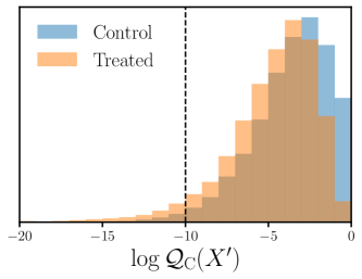
Figure 5: Distribution of $\log\mathcal{Q}_{\rm C}(X^{\prime})$ evaluated for covariate values in the control (blue) and treated (orange) sample. For a given set of covariate values, $X^{\prime}$ we evaluate $\log\mathcal{Q}_{\rm C}(X^{\prime})$ and $\log\mathcal{Q}_{\rm T}(X^{\prime})$. If both are above a conservative threshold (black dashed), we consider it within the support of our treated and control sample. Otherwise, we consider it outside of the support and refrain from evaluating CausalFlow on $X^{\prime}$.

Appendix B Covariate Support

CausalFlow can evaluate the CATE at any given value of the covariates within the support of the treated and control data, i.e. the given covariate is within the covariate distribution of the treated and control groups. CausalFlow is based on normalizing flows $q_{T}$ and $q_{C}$, trained on the treated and control data, respectively. So evaluating the CATE for any covariate outside their support would mean evaluating $q_{T}$ and $q_{C}$ beyond the covariate distribution they were trained on, i.e. extrapolation. The accuracy of CausalFlow is not be guaranteed in this regime. In this work, we avoid this scenario by only evaluating CausalFlow on covariate values classified as being within our treated and control distributions.

For the classification, we train two additional normalizing flows, $\mathcal{Q}^{T}(X)$ and $\mathcal{Q}^{C}(X)$, that estimate the distribution of X (community properties) of the treated and control samples. We follow roughly the same training procedure outline in Appendix A; however, unlike $q_{T}$ and $q_{C}$, $\mathcal{Q}_{\rm T}$ and $\mathcal{Q}_{\rm C}$ are not conditional distributions. For a given coviarate $X^{\prime}$, we evaluate the log probabilities $\log\mathcal{Q}_{\rm T}(X^{\prime})$ and $\log\mathcal{Q}_{\rm C}(X^{\prime})$. If both are above the threshold -10, we classify $X^{\prime}$ as within the treated and control support and proceed with evaluating CausalFlow. Otherwise, we classify $X^{\prime}$ as outside of the support. The threshold log probability value is empirically determined and conservatively set to correspond to the $\sim$1 percentile of the log probability distribution. We illustrate this in Figure 5, where we present the distribution of $\log\mathcal{Q}_{\rm C}(X^{\prime})$ values evaluated on the control (blue) and treated (orange) sample. We mark our threshold in black dashed. Our approach for classifying out-of-distribution covariate values is similar to methods for outlier detection (e.g. Liang et al., 2023; Böhm et al., 2023).

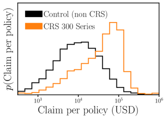
Figure 6: The distribution of total insurance claim per policy for non CRS communities (black) and CRS communities that mainly participate in the 300 Series activities (orange). The distribution qualitatively show that the outreach component of the CRS increases claims overall. The outreach activities provide guidance for the community on successfully filing claims. Based on a comparison of these two sets of communities in Appendix C, we find that the outreach component alone increases claims by $\sim$$9,780 USD per policy. We correct for this effect in the CATE in Eq. 4 to derive CATE’, the CRS savings.

Appendix C Impact of Outreach on CRS Savings

The CRS includes an outreach component where communities are informed how to successfully file their flood loss claims. The outreach itself would not impact actual flood looses. Yet, we expect this outreach to increase the total insurance claims per policy for communities in the CRS. If uncorrected, this would lead to an overall underestimation of the savings from the CRS program. Since our primary goal is to accurately measure the impact of the CRS on flood losses, we correct for this effect. Below, we describe how we estimate the effect of outreach alone.

FEMA compiles a CRS Communities Credit File data set, which provides detailed information on the points each CRS community receives for how effectively they implement the various CRS activities. Following a request to FEMA, we received access to these scores over the years 2010 to 2020 and cross-matched the scores to entries in our NFIP Flood Losses dataset (Section 2). The activities are categorized into 4 sets of activities: 300, 400, 500, and 600 series. They refer to activities for public information, mapping and regulations, flood damage reduction, and warning and response, respectively. This means that we can isolate the effect of outreach by comparing the insurance claims of CRS communities that primarily participate in the 300 activities to our control group, the non-CRS communities.

We first select communities in the CRS that participate in the 300 activities and score below 10% on the 400, 500, and 600 activities. These are communities that participate in outreach activities but do not effectively implement other flood management activities. This “CRS 300 Series” sample contains 36 zipcodes with 1955 entries. In Figure 6, we compare the distribution of total insurance claims per policy of this sample (orange) to the distribution of our control group (black). The comparison reveals that communities participating in outreach have significantly higher insurance claims per policy than the control sample.

To quality the effect of outreach more accurately, we take a similar approach as CausalFlow. For each entry in the “CRS 300 Series” sample with covariate values, $X^{\prime}$, we compute the expected insurance claim per policy if the entry was in the control group: $E[\,Y\,|\,X^{\prime},T=0]$ (Eq. 1). We use the normalizing flow, $q_{\rm C}$, from CausalFlow, with the same procedure as Eq. 3. We then calculate the difference between the actual insurance claim of the entry and the expected control value: $Y^{\prime}-E[\,Y\,|\,X^{\prime},T=0]$. The median value of the effect in the CRS 300 Series sample is $9,780 USD.

Our estimate confirms that the outreach component of the CRS indeed significantly increases the total insurance claims per policy. In principle, if there were more communities in the CRS that only participated in the 300 activities, we could estimate the effect of outreach as a function of the covariates using the same approach as CausalFlow. However, given our limited sample size, we examine the effect as a function of each covariate. We find no significant trends. Therefore, we use the median value as a fixed correction for the effect of outreach on the CRS savings.

Appendix D Community Typologies

With CausalFlow, we can examine the effectiveness of flood management activities (CATE) as a function of our 7 covariates: income, population, diversity, preciptation, flood risk, renter fraction, and educational attainment. A 7 dimensional covariate space, however, is challenging to interpret. Instead, we systematize our results by examining the CATE for a fixed set of 27 communities typologies defined by a permutation of income, population, and diversity.

The flood planning literature has shown that income, population, and diversity can explain uneven flood damage and loss exposure, as well as differing capabilities in preparing for and recovering from floods. For instance, Tate et al. (2021) illustrated that social vulnerability is a crucial indicator of flood exposure. Where population, race/ethnicity, and socioeconomic status have been found as the main components of such social vulnerability in relation to natural hazards  (Cutter & Finch, 2008). Previous work has also found that community income and race/ethnicity are associated with disproportionate flood impacts and unequal recovery  (Tate et al., 2021; Wing et al., 2022). The contribution of population, income, and race/ethnicity to the communities’ vulnerability vary significantly across counties (Cutter et al., 2003), so we define our community typologies using all of three characteristics.

	Low	Mid	High
Median Income (USD)	40,000	60,000	90,000
Population	2,500	12,000	30,000
Diversity Fraction	0.05	0.15	0.4

Table 1: Income, population, and diversity fraction values used to define the 27 community typologies for which we examine the CRS savings. For the typologies, we use all possible permutations of the low, mid, and high values.

For the actual income, population, and diversity values of the community typologies, we use values that roughly correspond to the 16, 50, and 84th percentiles of the full data set. In Table 1, we list the low, mid, and high income, population, and diversity fraction values used in this work. We take all possible permutations of the values to define $3\times 3\times 3=27$ community typologies.

In addition to income, population and diversity, we also determine the fiducial values of the other covariates for the 27 typologies. For each typology, we first select communities in our full data set with similar income, population and diversity. Afterwards set the fiducial covariate value of the typology as the median precipitation, flood risk, renter fraction, and educational attainment values of the selected communities. By taking the median values, we select the covariate valuesto form each typology.

Appendix E High Population, High Diversity, Mid to High Income

In Figure 7, we examine the geospatial distribution of high population, high diversity, and mid to high income communities (orange) compared to the rest of the communities in our data set (gray). The communities are highly localized and adjacent to the major cities that we labeled for reference. This localization suggests that these communities are in major urban areas.

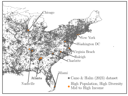
Figure 7: We highlight the communities in our data set (gray) that have high population, high diveristy, and mid to high income (orange). For reference, we mark the location of major cities near these communities. Compared to other communities in the data set, these communities are clearly located in major urban areas.

References

- Abadie & Gardeazabal (2003) Abadie A., Gardeazabal J., 2003, American Economic Review, 93, 113
- Abadie et al. (2010) Abadie A., Diamond A., Hainmueller J., 2010, Journal of the American Statistical Association, 105, 493
- Akiba et al. (2019) Akiba T., Sano S., Yanase T., Ohta T., Koyama M., 2019, in Proceedings of the 25th ACM SIGKDD international conference on knowledge discovery & data mining. pp 2623–2631
- Alderman et al. (2012) Alderman K., Turner L. R., Tong S., 2012, Environment International, 47, 37
- Alfieri et al. (2016) Alfieri L., Feyen L., Di Baldassarre G., 2016, Climatic Change, 136, 507
- Alsing et al. (2019) Alsing J., Charnock T., Feeney S., Wandelt B., 2019, MNRAS, 488, 4440
- Angrist (1990) Angrist J. D., 1990, The American Economic Review, 80, 313
- Asche (2013) Asche E. A., 2013, PhD thesis, University of California, Santa Barbara, United States – California
- Bevacqua et al. (2019) Bevacqua E., Maraun D., Vousdoukas M. I., Voukouvalas E., Vrac M., Mentaschi L., Widmann M., 2019, Science Advances, 5, eaaw5531
- Böhm et al. (2023) Böhm V., Kim A. G., Juneau S., 2023, arXiv e-prints, p. arXiv:2308.00752
- Brody et al. (2009) Brody S. D., Zahran S., Highfield W. E., Bernhardt S. P., Vedlitz A., 2009, Risk Analysis: An Official Publication of the Society for Risk Analysis, 29, 912
- Brouwer et al. (2007) Brouwer R., Akter S., Brander L., Haque E., 2007, Risk Analysis, 27, 313
- Cutter & Finch (2008) Cutter S. L., Finch C., 2008, Proceedings of the National Academy of Sciences, 105, 2301
- Cutter et al. (2003) Cutter S. L., Boruff B. J., Shirley W. L., 2003, Social Science Quarterly, 84, 242
- Davlasheridze et al. (2013) Davlasheridze M., Fisher-Vanden K., Klaiber H., 2013, 2013 Annual Meeting, August 4-6, 2013, Washington, D.C. 150196, The Higher Order Impacts of Hurricane: Evidence from County Level Analysis. Agricultural and Applied Economics Association
- Deegan (2007) Deegan M., 2007, Exploring U.S. Flood Mitigation Policies: A Feedback View of System Behavior. Rockefeller College of Public Affairs and Policy, Department of Public Administration and Policy
- Emrich et al. (2020) Emrich C. T., Tate E., Larson S. E., Zhou Y., 2020, Environmental Hazards, 19, 228
- FEMA (2018) FEMA 2018, An Affordability Framework for the National Flood Insurance Program | PreventionWeb, https://www.preventionweb.net/publication/affordability-framework-national-flood-insurance-program
- FEMA (2021) FEMA 2021, Community Rating System | FEMA.Gov, https://www.fema.gov/fact-sheet/community-rating-system
- Fan & Davlasheridze (2014) Fan Q., Davlasheridze M., eds, 2014, Evaluating the Effectiveness of Flood Mitigation Policies in the U.S, doi:10.22004/ag.econ.169399.
- Flores et al. (2023) Flores A. B., Collins T. W., Grineski S. E., Amodeo M., Porter J. R., Sampson C. C., Wing O., 2023, Annals of the American Association of Geographers, 113, 240
- Gonçalves et al. (2020) Gonçalves P. J., et al., 2020, eLife, 9, e56261
- Gourevitch & Pinter (2023) Gourevitch J., Pinter N., 2023, Environmental Research Letters
- Graham et al. (2019) Graham H., White P., Cotton J., McManus S., 2019, International Journal of Environmental Research and Public Health, 16, 3256
- Greenberg et al. (2019) Greenberg D. S., Nonnenmacher M., Macke J. H., 2019, Automatic Posterior Transformation for Likelihood-Free Inference
- Hahn & Melchior (2022) Hahn C., Melchior P., 2022, ApJ accepted, p. arXiv:2203.07391
- Haque (2021) Haque A. N., 2021, International Journal of Disaster Risk Reduction, 64, 102534
- Highfield & Brody (2017) Highfield W. E., Brody S. D., 2017, International Journal of Disaster Risk Reduction, 21, 396
- Jang & Chang (2022) Jang J.-H., Chang T.-H., 2022, Journal of Hydrology, 606, 127446
- Jongman et al. (2014) Jongman B., et al., 2014, Nature Climate Change, 4, 264
- Kingma & Ba (2017) Kingma D. P., Ba J., 2017, arXiv:1412.6980 [cs]
- Kirezci et al. (2020) Kirezci E., Young I. R., Ranasinghe R., Muis S., Nicholls R. J., Lincke D., Hinkel J., 2020, Scientific Reports, 10, 11629
- Knighton et al. (2020) Knighton J., Buchanan B., Guzman C., Elliott R., White E., Rahm B., 2020, Journal of Environmental Management, 272, 111051
- Kousky & Michel-Kerjan (2017) Kousky C., Michel-Kerjan E., 2017, Journal of Risk and Insurance, 84, 819
- Kousky et al. (2020) Kousky C., Kunreuther H., LaCour-Little M., Wachter S., 2020, Journal of Housing Research, 29, S3
- Lakshminarayanan et al. (2016) Lakshminarayanan B., Pritzel A., Blundell C., 2016, arXiv e-prints, p. arXiv:1612.01474
- Lemos et al. (2023) Lemos P., Coogan A., Hezaveh Y., Perreault-Levasseur L., 2023, Sampling-Based Accuracy Testing of Posterior Estimators for General Inference, https://arxiv.org/abs/2302.03026v1
- Li (2012) Li J., 2012
- Liang et al. (2023) Liang Y., Melchior P., Hahn C., Shen J., Goulding A., Ward C., 2023, arXiv e-prints, p. arXiv:2307.07664
- Mearns & Norton (2010) Mearns R., Norton A., 2010, Social Dimensions of Climate Change : Equity and Vulnerability in a Warming World. World Bank, doi:10.1596/978-0-8213-7887-8
- Michel-Kerjan & Kousky (2010) Michel-Kerjan E. O., Kousky C., 2010, Journal of Risk and Insurance, 77, 369
- Miguel & Kremer (2004) Miguel E., Kremer M., 2004, Econometrica, 72, 159
- Mitchell et al. (2015) Mitchell G., Norman P., Mullin K., 2015, Environmental Research Letters, 10, 105009
- NOAA (2014) NOAA 2014, Flood FAQ, https://www.nssl.noaa.gov/education/svrwx101/floods/faq/
- Papamakarios et al. (2018) Papamakarios G., Pavlakou T., Murray I., 2018, Masked Autoregressive Flow for Density Estimation (arXiv:1705.07057)
- Pasquier et al. (2022) Pasquier U., Vahmani P., Jones A. D., 2022, Water, 14, 3143
- Peek-Asa et al. (2012) Peek-Asa C., Ramirez M., Young T., Cao Y., 2012, Prehospital and Disaster Medicine, 27, 503
- Posey (2008) Posey J., 2008, Coping with Climate Change: Toward a Theory of Adaptive Capacity. Rutgers The State University of New Jersey, School of Graduate Studies
- Ranganathan & Bratman (2021) Ranganathan M., Bratman E., 2021, Antipode, 53, 115
- Reuters (2022) Reuters 2022, Reuters
- Rodell & Li (2023) Rodell M., Li B., 2023, Nature Water, 1, 241
- Rosenbaum & Rubin (1983) Rosenbaum P. R., Rubin D. B., 1983, Biometrika, 70, 41
- Siders & Keenan (2020) Siders A. R., Keenan J. M., 2020, Ocean & Coastal Management, 183, 105023
- Simpson et al. (2022) Simpson N. P., et al., 2022, Nature Climate Change, 12, 210
- Tabak & Turner (2013) Tabak E. G., Turner C. V., 2013, Communications on Pure and Applied Mathematics, 66, 145
- Tabak & Vanden-Eijnden (2010) Tabak E. G., Vanden-Eijnden E., 2010, Communications in Mathematical Sciences, 8, 217
- Talts et al. (2020) Talts S., Betancourt M., Simpson D., Vehtari A., Gelman A., 2020, arXiv:1804.06788 [stat]
- Tate et al. (2021) Tate E., Rahman M. A., Emrich C. T., Sampson C. C., 2021, Natural Hazards, 106, 435
- Tejero-Cantero et al. (2020) Tejero-Cantero A., Boelts J., Deistler M., Lueckmann J.-M., Durkan C., Gonçalves P. J., Greenberg D. S., Macke J. H., 2020, Journal of Open Source Software, 5, 2505
- Wahl et al. (2015) Wahl T., Jain S., Bender J., Meyers S. D., Luther M. E., 2015, Nature Climate Change, 5, 1093
- Walker-Springett et al. (2017) Walker-Springett K., Butler C., Adger W. N., 2017, Health & Place, 43, 66
- Wing et al. (2020) Wing O. E. J., Pinter N., Bates P. D., Kousky C., 2020, Nature Communications, 11, 1444
- Wing et al. (2022) Wing O. E. J., et al., 2022, Nature Climate Change, 12, 156
- Xu et al. (2023) Xu K., Zhuang Y., Bin L., Wang C., Tian F., 2023, Journal of Hydrology, 617, 129166
- Yang et al. (2022) Yang Q., et al., 2022, Bulletin of the American Meteorological Society, 103, E791