Light-Curve Structure and $\mbox{H}{\alpha}$ Line Formation in the Tidal Disruption Event AT 2019azh

Abstract

AT 2019azh is a H+He tidal disruption event (TDE) with one of the most extensive ultraviolet and optical datasets available to date. We present our photometric and spectroscopic observations of this event starting several weeks before and out to approximately two years after $g$-band peak brightness and combine them with public photometric data. This extensive dataset robustly reveals a change in the light-curve slope and a bump in the rising light curve of a TDE for the first time, which may indicate more than one dominant emission mechanism contributing to the pre-peak light curve. We further confirm the relation seen in previous TDEs whereby the redder emission peaks later than the bluer emission. The post-peak bolometric light curve of AT 2019azh is better described by an exponential decline than by the canonical $t^{-5/3}$ (and in fact any) power-law decline. We find a possible mid-infrared excess around peak optical luminosity, but cannot determine its origin. In addition, we provide the earliest measurements of the $\mbox{H}{\alpha}$ emission-line evolution and find no significant time delay between the peak of the $V$-band light curve and that of the $\mbox{H}{\alpha}$ luminosity. These results can be used to constrain future models of TDE line formation and emission mechanisms in general. More pre-peak 1–2 day cadence observations of TDEs are required to determine whether the characteristics observed here are common among TDEs. More importantly, detailed emission models are needed to fully exploit such observations for understanding the emission physics of TDEs.

1 Introduction

Supermassive black holes (SMBHs), with masses of $\gtrsim 10^{6}\,\textrm{\,M}_{\odot}$, are thought to reside in the center of most (if not all) large galaxies in the local Universe. While some SMBHs, known as active galactic nuclei (AGNs), accrete material that emits radiation, the majority are quiescent (e.g., Greene & Ho, 2007; Mullaney et al., 2013) and thus difficult to study.

One of the few probes that can be used to study inactive SMBHs is the emission produced in a tidal disruption event (TDE). A TDE occurs when a star passes close enough to an SMBH for tidal forces to surpass the star’s self-gravity, causing its disruption. In a full disruption, the star is torn apart and approximately half of it becomes gravitationally bound to the SMBH and eventually accretes onto it (Rees, 1988; Evans & Kochanek, 1989; Phinney, 1989).

This transient phenomenon can not only serve to confirm the presence of an SMBH but also offers a promising tool for constraining its mass and perhaps even spin (e.g., Leloudas et al., 2016). As such, TDEs can potentially provide a more complete picture of the SMBH population. This can, in turn, help address some of the open questions regarding SMBHs, from accretion physics through their sub- and super-Eddington growth mechanisms, to their scaling relations with global galaxy properties (such as the famous $M$–$\sigma$ relation; e.g., Kormendy & Ho 2013). However, a main unresolved challenge lies in mapping TDE emission properties to SMBH characteristics.

The first discovered TDEs were searched for and detected in X-ray observations (e.g., Bade et al. 1996; Komossa & Greiner 1999; Cappelluti et al. 2009; Maksym et al. 2014; see Saxton et al. 2020 for a recent review), as the transient accretion disk was expected to emit at these wavelengths. However, in recent years, wide-field optical transient surveys have been discovering a growing number of TDEs in the optical bands, which are also bright in ultraviolet (UV) wavelengths (e.g., Gezari et al. 2006; van Velzen et al. 2011; Gezari et al. 2012; Arcavi et al. 2014; see van Velzen et al. 2020 and Gezari 2021 for recent reviews). This surprising discovery has prompted work on theoretical models of TDEs to explain the optical/UV emission properties of these events.

Two main mechanisms for producing optical/UV emission in TDEs have been proposed. The first is the reprocessing of X-ray emission from an accretion disk by optically thick material surrounding the disk (e.g., Guillochon et al., 2014; Roth et al., 2016; Dai et al., 2018). The second model attributes the optical/UV emission to shocks formed between stellar debris streams as they collide around apocenter before circularizing to form an accretion disk (Piran et al., 2015).

UV/optical TDEs are characterized by a luminous peak with a typical absolute magnitude of $\sim-20$ in the optical (a few events have been found down to peak magnitudes of $\sim-17$), rise timescales of days to weeks, and a smooth decline in the light curve lasting weeks to years (e.g., van Velzen et al., 2020, 2021). The blackbody temperature of these events remains high and approximately constant at $T\approx 10^{4}$ K (e.g., Gezari et al., 2012; Arcavi et al., 2014; van Velzen et al., 2020). Their bolometric luminosity sometimes follows a decline rate consistent with a $t^{-5/3}$ power law, which aligns with theoretical expectations for the mass return rate (Rees, 1988; Evans & Kochanek, 1989; Phinney, 1989).

Spectroscopically, UV/optical TDEs show a strong blue continuum with broad ($\sim 10^{4}\,\textrm{\,km s}^{-1}$) He II $\lambda$4686 (Gezari et al., 2012; Arcavi et al., 2014) and/or broad Balmer emission lines (e.g., Arcavi et al., 2014; Gezari et al., 2015; Hung et al., 2017), denoted H- He- or H+He-TDEs, accordingly (van Velzen et al., 2021). The width of the emission lines was initially attributed to Doppler broadening (Ulmer, 1999; Bogdanović et al., 2004; Guillochon & Ramirez-Ruiz, 2013). However, it was later suggested that at least some of the line broadening is caused by electron scattering (Roth & Kasen, 2018). Some TDE spectra also exhibit He I $\lambda$5876 and/or heavier elements, such as [O III] $\lambda$5007 and N III $\lambda\lambda$4100, 4640 (sometimes blended with He II $\lambda$4686; Blagorodnova et al. 2017; Onori et al. 2019; Leloudas et al. 2019). Some of these lines have been attributed to the Bowen fluorescence mechanism (Bowen, 1934), whereby extreme UV photons generate a specific cascade of lines. TDEs showing these lines are known as “Bowen TDEs.”

Some UV/optical TDEs are accompanied by X-ray and/or radio emission (e.g., Brown et al., 2017; Cendes et al., 2022; Liu et al., 2022; Sfaradi et al., 2022; Bu et al., 2023). The X-rays are attributed to direct accretion emission, while the source of the radio emission is debated. It has been suggested to originate in outflows (Alexander et al., 2016), jets (van Velzen et al., 2016), and in the interaction between the unbound material and the interstellar medium (Krolik et al., 2016). In addition, delayed radio flares have recently been discovered to occur years after the optical peak in a few TDEs (Horesh et al., 2021). Their nature is also debated.

Here, we present and analyze extensive optical and UV observations, and available mid-infrared (MIR) observations, of the TDE AT 2019azh. X-ray, UV, and optical observations of this event were studied by Hinkle et al. (2021a), van Velzen et al. (2021), Liu et al. (2022), and Hammerstein et al. (2023). Delayed radio emission from it was examined by Sfaradi et al. (2022). Spectropolarimetry of AT 2019azh was studied by Leloudas et al. (2022) and found to have the lowest polarization among the sample of TDEs studied.

We complement published optical and UV data of AT 2019azh with our own. The combined optical and UV dataset presented here makes AT 2019azh one of the best-observed TDEs so far at these wavelengths, both photometrically and spectroscopically. We describe our observations in Section 2 and our analysis in Section 3, discuss our results in Section 4, and summarize in Section 5. We assume a flat $\Lambda$CDM cosmology, with $H_{0}=69.6$ $\textrm{\,km s}^{-1}$ Mpc^-1, $\Omega_{m}=0.286$, and $\Omega_{\Lambda}=0.714$ (Wright, 2006; Bennett et al., 2014).

2 Observations & Data Reduction

2.1 Discovery and Classification

AT 2019azh was discovered on February 22, 2019, 00:28:48 (UTC dates are used throughout this paper) (MJD 58536.02; Stanek, 2019) by the All-Sky Automated Survey for Supernovae (ASAS-SN; Kochanek et al., 2017) as ASASSN-19dj with a $g$-band apparent magnitude of $\sim 16.2$. The event was also detected by the Gaia photometric science alert team (Hodgkin et al., 2021) as Gaia19bvo, and by the Zwicky Transient Facility (ZTF; Bellm et al., 2019) as ZTF17aaazdba and ZTF18achzddr. The location of the event (Gaia J2000 coordinates $\alpha=08^{\rm hr}13^{\rm m}16.96^{\rm s}$, $\delta=+22^{\circ}38^{\prime}53.99^{\prime\prime}$) is consistent with the center of the nearby galaxy KUG 0810+227 which has a redshift of $z=0.0222240\pm 0.0000071$ (Almeida et al., 2023), corresponding to a luminosity distance of 96.6 Mpc. This galaxy was preselected by French & Zabludoff (2018) as a possible TDE host given its post-starburst properties (Arcavi et al., 2014).

The first few spectra of AT 2019azh showed a strong blue continuum without obvious features (Barbarino et al., 2019; Heikkila et al., 2019). The event was later classified as a TDE by van Velzen et al. (2019), based on its brightness, high blackbody temperature of $\sim 30,000$ K, a position consistent with the center of the galaxy (with an angular offset between the ZTF coordinates of the event and the host nucleus of $0.07\arcsec\pm 0.31\arcsec$), multiple spectra showing a strong blue continuum, and lack of spectroscopic features associated with a supernova (SN) or AGN.

2.2 Photometry

We obtained optical follow-up imaging of AT 2019azh with the Las Cumbres Observatory (Brown et al., 2013) global network of 1 m telescopes starting on MJD 58537.06 in the $BgVri$ bands. Standard image processing was performed using the BANZAI automated pipeline (McCully et al., 2018). We combine our set of images with that of Hinkle et al. (2021a) and perform reference-subtraction to remove host-galaxy contamination using the High Order Transform of PSF ANd Template Subtraction algorithm (HOTPANTS; Alard & Lupton, 1998; Alard, 2000; Becker, 2015) implemented by the lcogtsnpipe image-subtraction pipeline (Valenti et al., 2016). We use Las Cumbres Observatory images taken at MJD 59131.40 ($\sim 596$ days after discovery), after the transient faded, as references. Photometry was calibrated to the Sloan Digital Sky Survey (SDSS) Data Release 14 (Abolfathi et al., 2018) for the $gri$ bands and to the AAVSO Photometric All-Sky Survey (APASS) Data Release 9 (Henden et al., 2016) for the $BV$ bands.

AT 2019azh was observed by all five ASAS-SN units in the $g$ band, with the first detection recorded at MJD 58529.12. We use the ASAS-SN host-subtracted photometry as provided by Hinkle et al. (2021a).

The Swope (Bowen & Vaughan, 1973) 1 m telescope at Las Campanas Observatory observed AT 2019azh in the $uBgVri$ filters starting at MJD 58549.10. We use the Swope host-subtracted photometry as provided by Hinkle et al. (2021a).

We retrieved host-subtracted photometry from the Asteroid Terrestrial-impact Last Alert System (ATLAS; Tonry et al., 2018; Smith et al., 2020) in its $c$ and $o$ bands using the ATLAS public forced photometry server. AT 2019azh was first detected by ATLAS on MJD 58529.37. More details regarding ATLAS data processing and photometry extraction can be found in Tonry et al. (2018) and Smith et al. (2020).

We retrieved ZTF host-subtracted photometry from the public ZTF forced-photometry server. The event was detected in the ZTF $g$ and $r$ bands starting from MJD 58512.26. A description of forced-photometry processing for ZTF can be found in Masci et al. (2019).

The Neil Gehrels Swift Observatory (hereafter, Swift; Roming et al., 2005) observed AT 2019azh with all its UltraViolet and Optical Telescope (UVOT) filters ($b$, $v$, $u$, $uvw1$, $uvm2$, and $uvw2$), starting on MJD 58544.76 (PIs Arcavi, Hinkle, and Gezari). We take the host-subtracted extinction-corrected UVOT photometry from Hinkle et al. (2021b), which incorporates the new UVOT calibrations not available in the earlier work by Hinkle et al. (2021a).

We retrieve the available MIR photometry obtained by the Wide-field Infrared Survey Explorer (WISE; Wright et al., 2010) NEOWISE Reactivation Releases (Mainzer et al., 2011, 2014) through the NASA/IPAC infrared science archive (IRSA). WISE obtains several images of each object during each observing phase (once every six months). We process these data using a custom Python script. The script filters out any individual observation identified as an upper limit and those with observational issues such as being obtained close to the sky position of the Moon or suffering from poor frame quality. Weighted averages for each visit are then calculated per filter. We estimate the host-galaxy flux and its uncertainty as the average and variance (respectively) of all pre-TDE observations and then subtract this flux from all observations.

Table 1: Host-subtracted and Milky Way extinction-corrected photometry and $3\sigma$ nondetection upper limits.

MJD	Phase (days)	Magnitude	Error	Filter	Source
58509.23	-55.93	$>19.66$	$\ldots$	g	ZTF
58509.28	-55.88	$>19.88$	$\ldots$	r	ZTF
58512.26	-52.90	18.86	0.05	$r$	ZTF
58522.18	-42.98	20.13	0.15	$g$	ZTF
58537.07	-28.09	16.19	0.02	$r$	Las Cumbres
58537.07	-28.09	15.69	0.09	$g$	Las Cumbres
58571.85	6.69	17.14	0.01	$W1$	WISE
58571.85	6.69	17.47	0.01	$W2$	WISE

Note. — This table is published in its entirety in the machine-readable format. A portion is shown here for guidance regarding its form and content.

We correct all optical and UV photometry for Milky Way extinction assuming a Cardelli et al. (1989) extinction law with $R_{\rm V}=3.1$ and Galactic extinction of $A_{\rm V}=0.122$ mag, as retrieved from the NASA Extragalactic Database (NED) using the Schlafly & Finkbeiner (2011) extinction map. We correct the WISE MIR photometry for extinction using the Fitzpatrick (1999) extinction law with the corresponding coefficients from Yuan et al. (2013). All photometry is presented in the AB system (Oke, 1974), except for the Las Cumbres $BV$-band data which are presented in the Vega system.

The photometry obtained here from Las Cumbres, ATLAS, and ZTF are presented in Table 1. This photometry, together with the ASAS-SN and Swope photometry from Hinkle et al. (2021a), and the Swift photometry from Hinkle et al. (2021b), is presented in Figure 1. The WISE photometry is also presented in Table 1 and in Figure 2. We present all phases relative to $g$-band peak brightness at MJD $58565.16\pm 0.62$ (as calculated in Section 3).

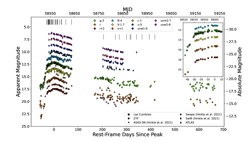
Figure 1: Milky Way extinction-corrected UV and optical light curves of AT 2019azh from Hinkle et al. (2021a, b) and this work. Arrows indicate 3$\sigma$ nondetection upper limits. Black vertical lines indicate epochs with spectroscopic data. The inset displays the rise of the light curve in five optical bands, where a “bump” appears $\sim-30$ days to $-10$ days from peak, and a sharp change in the slope of the rise is seen at $\sim-30$ days from peak.

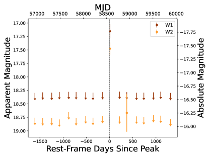
Figure 2: Milky Way extinction-corrected MIR light curves of AT 2019azh from WISE in days relative to the $g$-band peak. Arrows indicate 3$\sigma$ nondetection upper limits and the dashed vertical line indicates the $g$-band peak.

2.3 Spectroscopy

We obtained spectroscopic observations using the FLOYDS spectrographs (Sand et al., 2011) mounted on the Las Cumbres Observatory 2 m Faulkes Telescope South (FTS) located at the Siding Spring Observatory in Australia and Faulkes Telescope North (FTN) located at the Haleakalā Observatory in Hawaii, the ESO Faint Object Spectrograph and Camera (EFOSC2; Buzzoni et al., 1984) mounted on the 3.58 m ESO New Technology Telescope (NTT) as part of the extended Public ESO Spectroscopic Survey for Transient Objects (ePESSTO), the Asiago Faint Object Spectrographic Camera (AFOSC) mounted on the Copernico 1.82 m Telescope in Asiago, Mount Ekar, the Intermediate-dispersion Spectrograph and Imaging System (ISIS) mounted on the 4.2 m William Herschel Telescope (WHT), the Wide field reimaging CCD camera (WFCCD) mounted on the duPont 2.5 m telescope at the Las Campanas Observatory, the Kast Double Spectrograph (Miller & Stone, 1994) mounted on the Shane 3 m telescope at Lick Observatory, and the Alhambra Faint Object Spectrograph and Camera (ALFOSC) mounted on the 2.56 m Nordic Optical Telescope (NOT) through the second NOT Un-biased Transient Survey (NUTS2) program.

The FLOYDS spectra were processed and reduced using a custom PYRAF-based pipeline. This pipeline, based on the Image Reduction and Analysis Facility (IRAF; Tody, 1986, 1993) framework, removes cosmic rays and performs wavelength and flux calibration and rectification, flat-field correction, and spectrum extraction.

The Copernico 1.82 m Telescope spectra were reduced using a custom reduction pipeline based on IRAF tasks. After bias and flat-field correction, spectra were extracted and wavelength calibrated. Nightly sensitivity functions were derived from observations of spectrophotometric standard stars (also used to derive the corrections for the telluric absorption bands).

The NTT spectra were reduced using the Python-based PESSTO pipeline (Smartt et al., 2015). This pipeline encompasses essential steps, including detector bias calibration, flat-field calibration, cosmic-ray removal, comparison-lamp frames, and wavelength and flux calibrations. The first NTT spectrum, obtained on MJD 58539.16, is publicly available on the Transient Name Server (Barbarino et al., 2019).

The WHT/ISIS spectrum was reduced using custom recipes executed in IRAF. The use of the medium-resolution gratings (R600B and R600R) results in a gap in wavelength coverage between the blue and red arms. Overscan correction, bias subtraction, flat-field correction, and cosmic-ray removal were performed. Wavelength calibration is derived from comparison-lamp frames taken at the same position to correct instrument flexure. The optimal extraction algorithm of Horne (1986) is used to extract the one-dimensional spectra. A photometric standard star was observed on the same night to derive the flux calibration.

Observations with the WFCCD on the 2.5 m du Pont telescope were obtained using a 1.65″ (150 micron) slit and the blue grism. Average seeing conditions were $\sim$0.5″. Data were reduced and calibrated using custom Python routines and standard star observations.

The Lick/Kast spectra were taken with the 600/4310 grism, the 300/7500 grating, and the D57 dichroic. All observations were made with the 2.0″ slit. This instrument configuration has a combined wavelength range of $\sim$3600–10,700 Å, and a spectral resolving power of $R\approx 800$. The data were reduced following standard techniques for CCD processing and spectrum extraction (Silverman et al., 2012) utilizing IRAF routines and custom Python and IDL codes. Low-order polynomial fits to comparison-lamp spectra were used to calibrate the wavelength scale, and small adjustments derived from night-sky lines in the target frames were applied. The spectra were flux calibrated and telluric corrected using observations of appropriate spectrophotometric standard stars observed on the same night, at similar airmasses, and with an identical instrument configuration.

The ALFOSC spectrum was reduced using the foscgui pipeline. The pipeline performs overscan, bias, and flat-field corrections; spectrum extraction; wavelength calibration; flux calibration; and removal of telluric features with IRAF tasks as well as removal of cosmic-ray artifacts using lacosmic (van Dokkum, 2001).

All spectra were obtained with the slit oriented at or near the parallactic angle to minimize slit losses due to atmospheric dispersion (Filippenko, 1982).

We retrieved the spectrum of the host galaxy from SDSS Data Release 18 (Almeida et al., 2023). The spectrum was obtained on October 30, 2003, and covers a wavelength range of 3700–9300 Å with a spectral resolution of $R\approx 2000$.

Table 2: Log of spectroscopic observations.

Phase (days)	Telescope/ Instrument	Slit Width (″)	Exposure Time (s)
-31	NOT/ALFOSC	1.3	900
-27	NTT/EFOSC2	1	300
-24	Copernico/AFOSC	1.69	1800
-23	Copernico/AFOSC	1.69	1500
-22	Copernico/AFOSC	1.69	1200
-21	duPont/WFCCD	1.65	2700
-19	Copernico/AFOSC	1.69	2400
-19	duPont/WFCCD	1.65	2700
-17	duPont/WFCCD	1.65	2700
-16	Copernico/AFOSC	1.69	1800
-11	Las Cumbres/FLOYDS	2	1200
-10	Las Cumbres/FLOYDS	2	1200
-10	Copernico/AFOSC	1.69	2700
-7	Lick 3 m/Kast	2	2400
-5	NTT/EFOSC2	1	900
-5	Las Cumbres/FLOYDS	2	1200
0	Las Cumbres/FLOYDS	2	1200
+6	Las Cumbres/FLOYDS	2	1200
+7	Lick 3 m/Kast	2	2400
+12	Las Cumbres/FLOYDS	2	1200
+14	Las Cumbres/FLOYDS	2	1200
+16	Las Cumbres/FLOYDS	2	1200
+16	duPont/WFCCD	1.65	2700
+23	Las Cumbres/FLOYDS	2	1200
+30	Las Cumbres/FLOYDS	2	1200
+32	Lick 3 m/Kast	2	1500
+49	Lick 3 m/Kast	2	1800
+73	Lick 3 m/Kast	2	1800
+205	Las Cumbres/FLOYDS	2	3600
+254	Las Cumbres/FLOYDS	2	3600
+270	Las Cumbres/FLOYDS	2	3600
+300	Las Cumbres/FLOYDS	2	3600
+315	WHT/ISIS	1	2700
+318	Las Cumbres/FLOYDS	2	3600
+341	Las Cumbres/FLOYDS	2	3600
+364	Las Cumbres/FLOYDS	2	3600
+394	Las Cumbres/FLOYDS	2	3600
+417	Las Cumbres/FLOYDS	2	3600

Note. — Phase is given in rest-frame days from $g$-band peak brightness.

We calibrate all spectra of AT 2019azh (except for the WHT spectrum, owing to its wavelength gap) and that of the host galaxy to photometry and correct the TDE spectra for Milky Way extinction using the pysynphot package (STScI Development Team, 2013).

A log of our spectroscopic observations is provided in Table 2; all spectra are presented in Figure 3 and will be made available through the Weizmann Interactive Supernova Data Repository (WISeREP; Yaron & Gal-Yam, 2012).

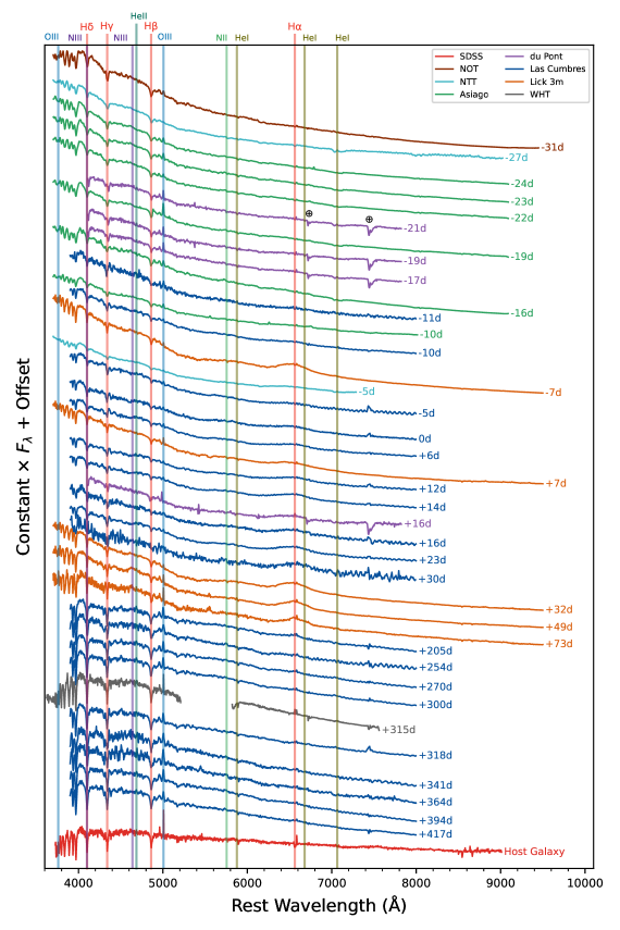
Figure 3: Spectroscopic evolution of AT 2019azh and the archival host-galaxy spectrum from SDSS, after photometric calibration and Galactic extinction correction (except for the WHT spectrum). Notable TDE features, such as broad $\mbox{H}{\alpha}$ and He II $\lambda$4686 emission lines, are evident in the spectra. We attribute the narrow Balmer absorption and narrow [O III] $\lambda$5007 emission lines, seen in all spectra, to the host galaxy. The phase of each spectrum in rest-frame days relative to the $g$-band light-curve peak is indicated and telluric lines are marked.

3 Analysis

3.1 Photometry

3.1.1 Light-Curve Rise

The high-cadence pre-peak observations of AT 2019azh allow us to identify structure in its early optical light curve. First, we identify an abrupt change in the rising slope of the $g$-band light curve at $\sim-30$ days relative to the peak. Second, a “bump” at $\sim-20$ days relative to the peak can be seen in the $BgVri$ bands. While subtle, it is present in all bands and hence we consider it significant. Such structure was not previously robustly identified in a TDE, in part owing to the lack of high-cadence pre-peak observations for most events. However, indications for early light-curve structure were seen in at least two TDEs which we discuss in Section 4.

3.1.2 Light-Curve Peak

We fit a second-order polynomial to the host-subtracted Las Cumbres optical photometry and Swift UV photometry (except for the Swift $uvw2$ data which does not cover enough of the rise to peak brightness) between MJD 58536 and 58596 to determine the peak time and magnitude in each band. The best-sampled light curve around peak is that in the $g$ band for which we find a peak time of MJD $58565.16\pm 0.62$ and peak absolute magnitude of $-19.85\pm 0.88$. We use this peak time as a reference for all phase information in this paper. We also check the cross-correlation offset between the $g$ light curve and the light curves in the bands mentioned above, in the same time range, using the PyCCF package (Peterson et al., 1998).

Table 3 details the peak time and apparent magnitude from the fit to peak in each band. Figure 4 illustrates the peak times of each band in relation to their central wavelengths. The $uvm2$, $uvw1$, and $u$-band central wavelengths and filter widths are taken from Poole et al. (2008), while the central wavelengths and filter widths for the rest of the bands are from the Las Cumbres Observatory website. We find a monotonic peak time delay in the redder bands compared to the bluer bands, in both the fit to peak and the cross-correlation delay methods. The offset values in the optical bands are consistent between the methods and are marginally consistent in the UV bands. Such a peak-time offset between bands has been documented in other TDEs and is discussed further in Section 4.

Table 3: Peak MJD and magnitude, determined by fitting a second-order polynomial to the Las Cumbres and Swift UV photometry around peak brightness.

Band	Central Wavelength (Å)	Filter Width (Å)	Peak MJD	Phase (days)	Peak Magnitude	Cross-Correlation Delay (days)
$uvm2$	2246	498	58554.71$\pm$5.20	-10.45$\pm$5.24	-20.50$\pm$0.03	$-3.97^{+3.17}_{-2.93}$
$uvw1$	2600	693	58553.25$\pm$4.62	-11.91$\pm$4.66	-20.29$\pm$0.02	$-3.98^{+2.97}_{-2.05}$
$u$	3465	785	58553.66$\pm$4.08	-11.5$\pm$4.12	-20.09$\pm$0.02	$-3.01^{+3.88}_{-2.05}$
$B$	4361	890	58565.18 $\pm$0.79	0.02$\pm$1.00	-19.73$\pm$0.03	$-0.08^{+2.84}_{-1.15}$
$g$	4770	1500	58565.16$\pm$0.62	0	-19.81$\pm$0.60	0
$V$	5448	840	58566.32$\pm$0.60	1.16$\pm$0.85	-19.71$\pm$0.02	$1.06^{+1.04}_{-1.84}$
$r$	6215	1390	58568.36$\pm$0.91	3.20$\pm$1.10	-19.57$\pm$0.72	$3.03^{+2.00}_{-2.97}$
$i$	7545	1290	58569.65$\pm$0.86	4.49$\pm$1.06	-19.38$\pm$0.49	$4.92^{+1.88}_{-1.18}$

Note. — Phases are given relative to the $g$-band peak, and cross-correlation delays are given relative to the $g$ light curve.

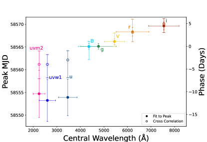
Figure 4: Light-curve peak MJD in various bands. Bluer bands peak earlier than redder bands. Filter widths are indicated with horizontal lines.

We find a significant MIR flare at 6.2 days after the $g$-band peak, with a $W1-W2$ color of $-0.32$ mag, which is well below the AGN threshold of $W1-W2=0.8$ determined by Stern et al. (2012).

We calculate the expected MIR flux of a blackbody with the best-fit temperature and radius from day 9.63 after $g$-band peak (the closest blackbody fit to the time of the WISE detections; see Section 3.1.3) using the synphot package (STScI Development Team, 2018) with the WISE $W1$ and $W2$ filter bandpasses from Wright et al. (2010). We find that such a blackbody would produce a $W1$ and $W2$ AB magnitude of $-16.32\pm 0.07$ (the difference between the $W1$ and $W2$ magnitudes is negligible at the assumed temperature of $2.46\pm 0.15\times 10^{4}$ K derived in Section 3.1.3). The MIR detection extinction-corrected $W1$ and $W2$ AB magnitudes are $-17.76\pm 0.13$ and $-17.45\pm 0.11$, respectively, which are $\sim 1.1$–1.5 mag brighter than the blackbody emission inferred from the optical and UV data. This excess may be due to a prompt dust echo, as observed, for example, by Newsome et al. (2023), but we cannot verify this without further data. We leave further analysis of the MIR emission from AT 2019azh to future work.

3.1.3 Blackbody Fits

We fit the UV/optical photometry of AT 2019azh with a blackbody spectrum through the SuperBol fitting package (Nicholl, 2018), which uses the least-squares fitting method. Here we exclude ATLAS observations since the $c$- and $o$-band filters overlap with other filters, making them not fully independent observations. We restrict the fitting to epochs with available UV observations, as this helps reduce systematic errors when fitting blackbodies hotter than $\sim 30,000$ K with optical data alone (Arcavi, 2022), while linearly interpolating the optical light curves where necessary. We then calculate the bolometric luminosity using the Stefan-Boltzmann law, $L_{\rm bol}=4\pi{R^{2}}\sigma_{\rm SB}{T^{4}}$, with $\sigma_{\rm SB}$ the Stefan-Boltzmann constant, and $R$ and $T$ the blackbody radius and temperature from the fit, respectively.

The evolution of the blackbody temperature, radius, and resulting bolometric luminosity are given in Table 4 and presented in Figure 5 in comparison to 15 other TDEs from van Velzen et al. (2021). As with other TDEs, AT 2019azh exhibits constant high ($\sim 25,000$ K) temperatures with values at the high end, but consistent with the sample of van Velzen et al. (2021). Its blackbody radius evolution is also consistent with that of other TDEs and falls in the middle of the comparison sample. The bolometric luminosity of AT 2019azh is on the high end of the comparison sample, but still consistent with it. Our results are also roughly consistent with those of Hinkle et al. (2021b), but we obtain slightly lower temperatures and bolometric luminosities, especially at late times, compared to them.

Table 4: Blackbody temperature and radius, and resulting bolometric luminosity.

Phase	$T_{\rm BB}$ ($10^{4}$ K)	$R_{\rm BB}$ ($10^{14}$ cm)	$L_{\rm bol}$ ($10^{44}\textrm{\,erg s}^{-1}$)
$-20.40$	2.55 $\pm$ 0.13	7.45 $\pm$ 0.43	1.66 $\pm$ 0.40
$-11.71$	2.75 $\pm$ 0.15	7.05 $\pm$ 0.45	2.03 $\pm$ 0.52
$-9.05$	2.83 $\pm$ 0.16	7.33 $\pm$ 0.45	2.46 $\pm$ 0.62
$-2.21$	2.49 $\pm$ 0.10	8.08 $\pm$ 0.38	1.80 $\pm$ 0.33
0.78	2.55 $\pm$ 0.12	7.91 $\pm$ 0.43	1.88 $\pm$ 0.40
2.91	2.54 $\pm$ 0.17	7.70 $\pm$ 0.63	1.77 $\pm$ 0.56
3.12	2.36 $\pm$ 0.16	7.98 $\pm$ 0.68	1.42 $\pm$ 0.45
9.63	2.46 $\pm$ 0.15	7.87 $\pm$ 0.56	1.61 $\pm$ 0.45
11.94	2.43 $\pm$ 0.15	7.93 $\pm$ 0.59	1.55 $\pm$ 0.44
15.46	2.51 $\pm$ 0.18	7.38 $\pm$ 0.63	1.55 $\pm$ 0.51
18.11	2.50 $\pm$ 0.17	7.36 $\pm$ 0.61	1.51 $\pm$ 0.49
24.37	2.56 $\pm$ 0.18	6.71 $\pm$ 0.56	1.38 $\pm$ 0.45
26.89	2.62 $\pm$ 0.19	6.46 $\pm$ 0.55	1.40 $\pm$ 0.47
30.20	2.68 $\pm$ 0.22	6.06 $\pm$ 0.57	1.34 $\pm$ 0.50
33.13	2.63 $\pm$ 0.21	5.93 $\pm$ 0.55	1.19 $\pm$ 0.44
35.18	2.10 $\pm$ 0.17	7.00 $\pm$ 0.70	0.68 $\pm$ 0.26
40.96	2.94 $\pm$ 0.28	4.93 $\pm$ 0.51	1.29 $\pm$ 0.56
44.01	2.97 $\pm$ 0.32	4.85 $\pm$ 0.56	1.30 $\pm$ 0.64
46.26	2.54 $\pm$ 0.19	5.91 $\pm$ 0.47	1.03 $\pm$ 0.35
53.17	2.85 $\pm$ 0.25	4.86 $\pm$ 0.47	1.10 $\pm$ 0.45
56.16	2.81 $\pm$ 0.25	4.79 $\pm$ 0.47	1.02 $\pm$ 0.41
59.28	2.98 $\pm$ 0.25	4.45 $\pm$ 0.40	1.10 $\pm$ 0.42
61.87	3.00 $\pm$ 0.28	4.34 $\pm$ 0.44	1.08 $\pm$ 0.45
65.26	3.02 $\pm$ 0.29	4.21 $\pm$ 0.44	1.05 $\pm$ 0.46
69.04	3.05 $\pm$ 0.26	4.03 $\pm$ 0.38	1.00 $\pm$ 0.39
73.11	2.84 $\pm$ 0.23	4.19 $\pm$ 0.38	0.81 $\pm$ 0.30
202.78	3.13 $\pm$ 0.40	1.49 $\pm$ 0.19	0.15 $\pm$ 0.09
222.05	2.88 $\pm$ 0.29	1.44 $\pm$ 0.15	0.10 $\pm$ 0.05
225.43	2.73 $\pm$ 0.28	1.52 $\pm$ 0.16	0.09 $\pm$ 0.04
229.48	2.32 $\pm$ 0.16	1.76 $\pm$ 0.14	0.06 $\pm$ 0.02
234.53	2.60 $\pm$ 0.33	1.52 $\pm$ 0.21	0.08 $\pm$ 0.04
261.73	2.68 $\pm$ 0.56	1.25 $\pm$ 0.26	0.06 $\pm$ 0.05
277.22	2.62 $\pm$ 0.39	1.26 $\pm$ 0.19	0.05 $\pm$ 0.04
285.05	2.63 $\pm$ 0.38	1.23 $\pm$ 0.19	0.05 $\pm$ 0.03

Note. — Phases are given relative to $g$-band peak brightness.

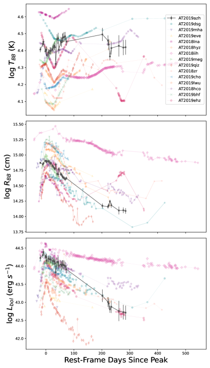
Figure 5: Blackbody temperature (top), radius (middle), and inferred bolometric luminosity (bottom) evolution obtained using SuperBol for AT 2019azh (black), compared to a sample of TDEs from van Velzen et al. (2021). The temperature, radius, and bolometric luminosity of AT 2019azh are consistent with those of other UV/optical TDEs. The van Velzen et al. (2021) measurements assume a parametric time evolution and hence are smoother.

We fit the post-peak bolometric light curve with a power law of the form $L\propto\left(\frac{t-t_{0}}{\tau}\right)^{-\alpha}$ and an exponential decline of the form $L{\propto}e^{-\frac{t-t_{0}}{\tau}}$. We perform the power-law fit in three different ways: once with the power-law index fixed to the canonical $\alpha=5/3$ value and free $t_{0}$, once with free $\alpha$ and fixed $t_{0}$ (set to the best-fit value of $-60$ days from peak, found by MOSFiT below), and once with free $\alpha$ and free $t_{0}$. The last fit requires an unphysical $t_{0}$ of order $10^{5}$ days before peak to match the data, and the other two power-law fits (yielding $\alpha=2.05\pm 0.11$ and $t_{0}=-41.98\pm 5.51$ days) are unable to match the data at all. The exponential decline, on the other hand, does match the data well. The different fits are shown in Figure 6. We conclude that the bolometric light-curve decline of AT 2019azh is better described by an exponential than a power law. Specifically, it does not fit the canonical $t^{-5/3}$ decline quoted for some TDEs.

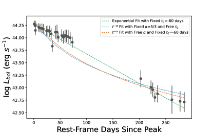
Figure 6: Power-law and exponential fits to the bolometric luminosity decline. The data are better represented by an exponential decline rather than a power law.

3.1.4 TDE Model Fits

As mentioned in Section 1, there are currently two main models for the source of UV/optical emission in TDEs: reprocessing of X-rays from a rapidly-formed accretion disk, and shock emission from debris stream collisions during the circularization process. We fit our photometry to the X-ray reprocessing model with the Modular Open Source Fitter for Transients (MOSFiT; Guillochon et al., 2018), and to the stream-collision model with the TDEMass package (Ryu et al., 2020).

The MOSFiT TDE model (Mockler et al., 2019) is based on hydrodynamical simulations for converting the mass-fallback rate from the disrupted star to a bolometric flux. This conversion is related to the accretion rate through the viscous timescale $T_{\rm viscous}$, and it assumes a constant efficiency parameter $\epsilon$. The reprocessing layer is assumed to be a simple blackbody photosphere with radius $R_{\rm phot}$.

The free parameters of the model are the BH mass ($M_{\rm BH}$); the mass of the disrupted star ($M_{\star}$); the viscous timescale ($T_{\rm viscous}$); the efficiency ($\epsilon$); the blackbody photospheric radius $R_{\rm phot}\propto R_{\rm ph,0}\times L^{l}$ (where $R_{\rm ph,0}$ and $l$ are free parameters and $L$ is the bolometric luminosity); the scaled impact parameter ($b$), which is a proxy for the physical impact parameter $\beta\equiv R_{\rm t}/R_{\rm p}$ (with $R_{\rm t}$ the tidal radius and $R_{\rm p}$ the orbit pericenter); the time of first fallback ($t_{\rm exp}$); the host-galaxy column density ($n_{\rm H}$); and a white-noise parameter ($\sigma$). We use the default priors from MOSFiT, as given by Mockler et al. (2019).

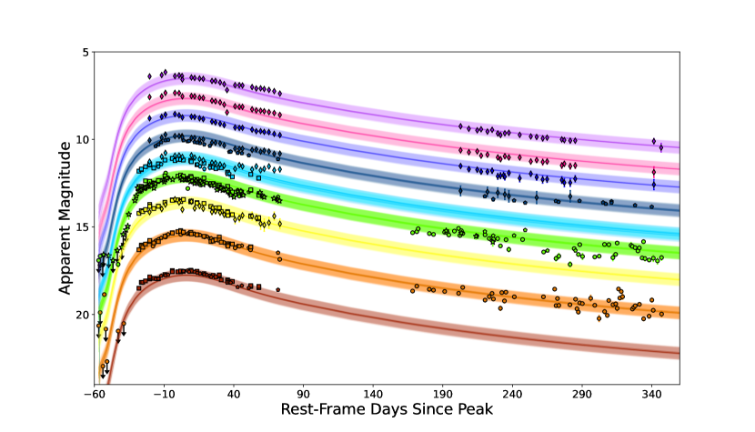
Figure 7: MOSFiT nested sampling fits to AT 2019azh photometry. Solid lines represent the medians of samples of light curves, while the shaded regions indicate the variance within each sample of models. Overall, the ensembles of models provide a reasonably good fit to the photometric data after peak brightness but do not accurately reproduce the rise to the peak. Arrows indicate 3$\sigma$ nondetection upper limits. Colors, markers, and offsets are the same as in Figure 1.

We utilize the Nested Sampling method, implemented by DYNESTY (Speagle, 2020), for the fit. As with the blackbody fits, here we also exclude the ATLAS bands. We further exclude observations more than 1 yr after discovery because the assumption of a blackbody photosphere made by MOSFiT might not be valid at such late times if the reprocessing material starts to become optically thin.

The model matches the post-peak observations reasonably well but does not accurately reproduce the rapid rise to the peak, as can be seen in Figure 7. Table 5 presents the best-fit parameters obtained from the fit; the posterior distributions, which are well converged, are displayed in Figure 12 in Appendix A. The efficiency parameter approaches its maximum allowed value, which affects the stellar mass parameter owing to their degeneracy (Mockler & Ramirez-Ruiz, 2021). The impact parameter is $b=0.99^{+0.01}_{-0.03}$, suggesting that the star is almost fully disrupted.

As Mockler et al. (2019) pointed out, this model includes several simplifications of the complex physics involved. For instance, assuming solar-composition polytropes instead of more realistic stellar density profiles that take into account the stellar metallicity, age, and evolutionary stage, could introduce systematic uncertainties in determining the stellar mass. Mockler et al. (2019) quantified these and other systematic uncertainties arising from some of the model simplifications, and we include these uncertainties in the total error estimates in Table 5.

Table 5: Best-fit parameters obtained from the MOSFiT fit with 1$\sigma$ confidence intervals.

Parameter	Best-Fit Value	Total Error	Units
log($M_{\rm BH}$)	$7.21^{+0.02}_{-0.02}$	$\pm 0.20$	$\textrm{\,M}_{\odot}$
$M_{\star}$	0.1000${}^{+0.0002}_{-0.0002}$	$\pm 0.66$	$\textrm{\,M}_{\odot}$
log($T_{\rm viscous}$)	$0.44^{+0.14}_{-0.42}$	$\pm 0.43$	d
log($\epsilon$)	$-0.47^{+0.05}_{-0.08}$	$\pm 0.68$
log($R_{\rm ph,0}$)	$0.38^{+0.07}_{-0.05}$	$\pm 0.4$
$l$	$1.72^{+0.05}_{-0.06}$	$\pm 0.2$
$b$	$0.99^{+0.01}_{-0.03}$	$\pm$0.35
$t_{\rm exp}$	$-6.95^{+1.24}_{-1.00}$	$\pm 15$	d
log($n_{\rm H}$)	$20.66^{+0.03}_{-0.04}$		cm-2
log($\sigma$)	$-0.45^{+0.01}_{-0.01}$

Note. — The “Total Error” column includes systematic errors estimated by Mockler et al. (2019) due to some of the simplifying assumptions in the model.

In TDEMass (Ryu et al., 2020), the mass of the disrupted star and the disrupting SMBH are estimated by numerically solving two nonlinear equations (Eqs. 11 and 12 of Ryu et al. 2020) and interpolating within precalculated tables of the peak bolometric luminosity ($L_{\rm obs}$) and the temperature at this peak ($T_{\rm obs}$). The equations include two parameters which determine the size and energy-dissipation area of the emitting region: $c_{1}$, related to the apocenter distance for the orbit of the most tightly bound debris, and $\Delta\Omega$, the solid angle of the area where shocks dissipate a significant amount of energy. The values of these parameters are not well constrained, and the default model values of $c_{1}=1$ and $\Delta\Omega=2\pi$ are assumed.

From our SuperBol fit, we find a peak luminosity of $L_{\rm obs}=2.46\pm 0.62\times 10^{44}$ $\textrm{\,erg s}^{-1}$ and a temperature at this peak of $T_{\rm obs}=28,300\pm 1550$ K. With these values we obtain from TDEMass a BH mass of $M_{\rm BH}=2.5^{+0.29}_{-0.24}\times 10^{6}\,\textrm{\,M}_{\odot}$ and a stellar mass of $M_{\star}=4.8^{+4}_{-2.5}\,\textrm{\,M}_{\odot}$. Figure 13 in Appendix B displays the degeneracy between these two parameters. We compare these results to those found through MOSFiT in Section 4, though we do not expect them to agree since each model assumes a different emission mechanism responsible for the observed light curve.

3.2 Spectroscopy

3.2.1 Coronal Emission Lines

We use a custom analysis code (Clark et al., in prep) to check for the presence of narrow [Fe VII], [Fe X], [Fe XI], and [Fe XIV] coronal emission lines in our spectra. Such lines are seen in extreme coronal line emitters (ECLE; e.g., Komossa et al., 2008; Wang et al., 2012; Yang et al., 2013), a subset of which is associated with TDEs (e.g., Onori et al., 2022; Clark et al., 2023; Short et al., 2023) occurring in gas-rich environments. We find no significant evidence for such features in any of our spectra.

3.2.2 Other Emission Lines

To identify and study the broad emission lines, we follow the spectral analysis process outlined by Charalampopoulos et al. (2022) for removing host-galaxy and continuum contributions to the emission-line profiles (after performing the photometric calibration and Galactic extinction correction as detailed in Section 2). We exclude from this analysis the duPont spectra to avoid telluric contamination, and all spectra taken after the seasonal gap (day 205 after peak and onward) given that the broad emission lines are very weak at such late times.

Table 6: $\mbox{H}{\alpha}$ luminosity, FWHM, and central wavelength offset of AT 2019azh.

Phase	$\mbox{H}{\alpha}$ Luminosity ($10^{40}\textrm{\,erg s}^{-1}$)	$\mbox{H}{\alpha}$ FWHM ($\textrm{\,km s}^{-1}$)	$\mbox{H}{\alpha}$ Central Wavelength Offset ($\textrm{\,km s}^{-1}$)
-31	1.88 $\pm$ 0.17	7044.25 $\pm$ 497.25	-475.83 $\pm$ 487.42
-27	1.88 $\pm$ 0.21	5925.27 $\pm$ 522.95	-466.12 $\pm$ 522.95
-24	2.15 $\pm$ 0.18	11240.37 $\pm$ 768.48	-4986.51 $\pm$ 768.48
-23	3.37 $\pm$ 0.21	9025.71 $\pm$ 424.88	-5735.38 $\pm$ 424.88
-22	3.31 $\pm$ 0.19	9451.13 $\pm$ 409.11	-6126.03 $\pm$ 409.11
-19	3.81 $\pm$ 0.14	8983.63 $\pm$ 248.32	-5662.58 $\pm$ 248.32
-16	6.40 $\pm$ 0.28	9018.48 $\pm$ 304.55	-5751.50 $\pm$ 304.55
-11	5.62 $\pm$ 0.23	9252.85 $\pm$ 294.55	-3340.03 $\pm$ 294.55
-10	7.14 $\pm$ 0.46	9125.29 $\pm$ 463.09	-3528.82 $\pm$ 463.09
-10	10.59 $\pm$ 0.23	8192.05 $\pm$ 135.60	-3488.98 $\pm$ 135.60
-7	12.63 $\pm$ 0.16	6002.88 $\pm$ 57.84	-1165.36 $\pm$ 57.84
-5	14.45 $\pm$ 0.36	7385.70 $\pm$ 147.60	-3145.95 $\pm$ 147.60
-5	13.69 $\pm$ 0.31	8090.10 $\pm$ 140.20	-2678.93 $\pm$ 140.20
0	15.43 $\pm$ 0.31	7478.12 $\pm$ 114.39	-2797.66 $\pm$ 114.39
6	14.56 $\pm$ 0.20	8052.00 $\pm$ 84.94	-2396.22 $\pm$ 84.94
7	11.84 $\pm$ 0.14	7629.80 $\pm$ 69.03	-2685.32 $\pm$ 69.03
12	10.18 $\pm$ 0.15	7446.41 $\pm$ 84.53	-1490.40 $\pm$ 84.53
14	13.39 $\pm$ 0.16	7506.35 $\pm$ 67.07	-1792.32 $\pm$ 67.07
16	7.72 $\pm$ 0.19	6329.29 $\pm$ 121.57	-1711.47 $\pm$ 121.57
23	9.80 $\pm$ 0.10	7384.67 $\pm$ 60.07	-1640.46 $\pm$ 60.07
30	10.26 $\pm$ 0.45	5941.76 $\pm$ 197.83	491.88 $\pm$ 197.83
32	7.19 $\pm$ 0.08	6026.94 $\pm$ 53.00	-1065.69 $\pm$ 53.00
49	6.38 $\pm$ 0.06	5491.54 $\pm$ 40.69	-166.10 $\pm$ 40.69
73	5.05 $\pm$ 0.11	4424.70 $\pm$ 71.28	664.59 $\pm$ 71.28

Note. — Phases are given relative to the $g$-band peak brightness.

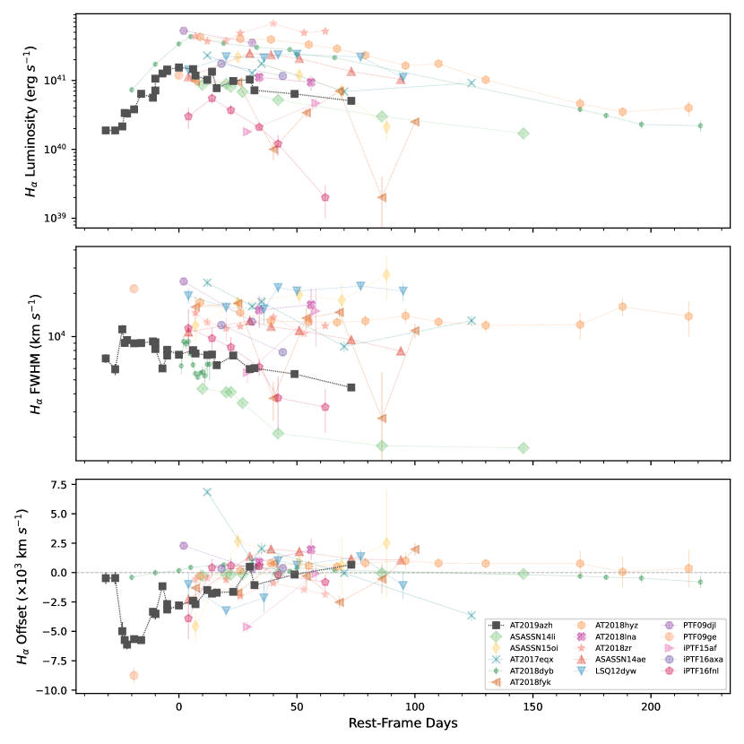
Figure 8: Evolution of $\mbox{H}{\alpha}$ line luminosity (top), FWHM (center), and central wavelength offset (bottom) of AT 2019azh (black), compared to that of a sample of 15 TDEs from Charalampopoulos et al. (2022). AT 2019azh is plotted relative to its $g$-band peak, while the comparison data are plotted relative to their peak or discovery date (see Charalampopoulos et al., 2022, for details).

First, we subtract the host-galaxy spectrum from each TDE spectrum after resampling the host spectrum to the wavelengths of the TDE spectrum using the SciPy interp1d function. Since different spectra are taken under different seeing conditions, and the TDE spectra are taken with varying slit widths and angles, while the SDSS host spectrum was obtained through a fiber, there will be different host-galaxy contributions to each TDE spectrum. Thus, it is impossible to completely remove host-galaxy emission from the TDE spectra. Here we attempt to minimize host-galaxy contamination, but some residuals likely remain (see below).

Next, we identify line-free regions in the host-subtracted spectra to fit and remove the spectral continuum using a third-order polynomial. We use line-free regions outlined by Charalampopoulos et al. (2022) as a basis, while tailoring them to match the AT 2019azh spectra. The selected line-free rest-frame wavelength ranges are 3900–4000 Å, 4220–4280 Å, 5100–5550 Å, 6000–6100 Å, and 6800–7000 Å.

An example of this spectral processing procedure, as performed on the spectrum from 14 days after peak brightness, is provided in Figure 14 in Appendix C. All spectra after host and continuum removal, for which this process was conducted, are presented in Figure 15 in Appendix C.

Broad emission lines of $\mbox{H}{\alpha}$, He II $\lambda$4686, and He I $\lambda$5876 are evident, as in other UV/optical TDEs (e.g., Gezari et al., 2012; Arcavi et al., 2014; Holoien et al., 2016). The broad He II $\lambda$4686 emission line appears already in the first spectrum, remains relatively strong and broad until the seasonal gap at 73 days after the light-curve peak, and weakens in the spectra obtained after the gap (see Figure 15 in Appendix C). The broad $\mbox{H}{\alpha}$ emission line strengthens at early times and later significantly weakens and narrows in the post-seasonal-gap spectra. This behavior was observed in some other TDEs (e.g., Gezari et al. 2012; Holoien et al. 2014, 2016), and is discussed further in Section 3.2.3.

In addition to the broad emission lines, narrow Balmer $\mbox{H}{\beta}$ and $\mbox{H}{\gamma}$ emission lines are seen in the host- and continuum-subtracted spectra. These lines likely originate from oversubtraction of the host-galaxy spectrum (as they also appear in the SDSS host spectrum as narrow absorption lines; see Figure 3). We also find a strong, narrow [O III] $\lambda$5007 absorption line in the host-subtracted spectra (see Figure 14 in Appendix C), which is probably also an oversubtracted host-galaxy emission line.

3.2.3 $\mbox{H}{\alpha}$ Line Evolution

Following Charalampopoulos et al. (2022), we quantify the evolution of the $\mbox{H}{\alpha}$ emission line, as it is a relatively isolated line. For each host- and continuum-subtracted spectrum, we fit the $\mbox{H}{\alpha}$ emission line with a Gaussian using the nonlinear least-squares method of the LMFIT package. We use the same initial guesses for the center (6563 Å) and width (150 Å, corresponding to a Doppler velocity of $\sim 10,000$ $\textrm{\,km s}^{-1}$), for all spectra. All Gaussian fits, after normalizing the peak of the feature, are shown in Figure 16 in Appendix C.

The evolution of the $\mbox{H}{\alpha}$ line luminosity is presented in the top panel of Figure 8, along with data from 15 other TDEs obtained from Charalampopoulos et al. (2022), which were measured using the same methodology as described here and is the largest sample of homogeneously analyzed TDE spectra to date. Around peak brightness, the $\mbox{H}{\alpha}$ luminosity is similar to those of the comparison sample. The post-peak slight decay of the $\mbox{H}{\alpha}$ luminosity is also consistent with the rest of the sample. However, the extensive pre-peak spectral observations of AT 2019azh reveal the initial formation of this emission line in a TDE for the first time. These observations can be used to constrain future models of spectral line formation in TDEs.

We also measure the evolution of the full width at half-maximum (FWHM) intensity of the Gaussian fits to the $\mbox{H}{\alpha}$ emission line of AT 2019azh, and compare them to those of the Charalampopoulos et al. (2022) sample in the middle panel of Figure 8. The FWHM of the $\mbox{H}{\alpha}$ emission line of AT 2019azh is similar to those of the Charalampopoulos et al. (2022) sample, and it shows a clear gradual decline.

Finally, in the bottom panel of Figure 8, we compare the evolution of the $\mbox{H}{\alpha}$ best-fit Gaussian central wavelength offset from the rest wavelength, with that of the same sample from Charalampopoulos et al. (2022). While the line centers of the first two spectra are consistent with zero offset, a blueshift rapidly develops and slowly returns back to zero offset within a few months. The magnitude of the offset is consistent with those of other events in the Charalampopoulos et al. (2022) sample, but AT 2019azh is the only event showing this kind of evolution.

The $\mbox{H}{\alpha}$ luminosity, FWHM, and central-wavelength offset values for AT 2019azh are presented in Table 6.

Charalampopoulos et al. (2022) showed that TDEs exhibit a time lag between their light curve (i.e., continuum emission) and $\mbox{H}{\alpha}$ luminosity peaks. Figure 9 compares the evolution of the $\mbox{H}{\alpha}$ luminosity and the $V$-band light curve for AT 2019azh. To determine the peak time of the $\mbox{H}{\alpha}$ line luminosity for AT 2019azh, we fit a second-order polynomial to the $\mbox{H}{\alpha}$ luminosity from $-18$ to +18 days since $g$-band peak and find that the peak occurred on MJD $58566.56\pm 1.58$, or $\Delta t=1.35\pm{1.45}$ days after the $V$-band light-curve peak.

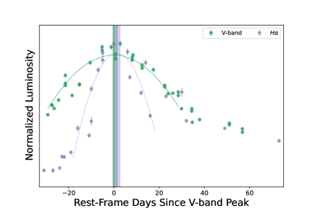
Figure 9: $\mbox{H}{\alpha}$ luminosity evolution (purple), compared to the $V$-band light curve of AT 2019azh (green). The colored dashed lines are the parabolic fits to the data around peak brightness, from which the peak times were determined. The vertical solid lines and shaded regions mark the peak times for the $V$-band and $\mbox{H}{\alpha}$ peaks, and their $1\sigma$ uncertainties, respectively. The $\mbox{H}{\alpha}$ peak time is consistent with that of the $V$-band peak.

4 Discussion

4.1 Spectroscopic Classification of AT 2019azh

In Figure 10 we compare the spectra around peak of AT 2019azh to those of the Bowen TDE AT 2018dyb (Leloudas et al., 2019), the H+He-TDE AT 2020wey (Charalampopoulos et al., 2023), which also showed a possible early light-curve bump, and AT 2019ahk, which does not show such structure despite having a very densely sampled early-time light curve (see below). AT 2019azh does not show N III $\lambda\lambda$4100, 4640 emission like those seen in AT 2018dyb, meaning it is not a Bowen TDE. Its broad H and He II $\lambda$4686 emission features are similar to those of AT 2020wey, making it an H+He-TDE. AT 2019ahk shows strong AGN-like narrow spectral emission lines, not seen in most TDEs, implying it might be a different type of flare.

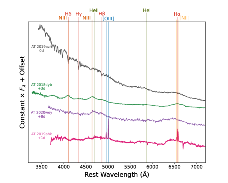
Figure 10: Spectral comparison around peak luminosity of AT 2019azh with the well-observed Bowen TDE AT 2018dyb (Leloudas et al., 2019), the H+He-TDE AT 2020wey (Charalampopoulos et al., 2023), which also showed possible early light-curve structure, and AT 2019ahk, which did not show such structure in its very densely-sampled light-curve rise. The similarity of the AT 2019azh spectrum to that of AT 2020wey classifies it as an H+He-TDE. The spectrum of AT 2019ahk displays distinctive narrow emission lines, implying it might be an AGN-related flare rather than a “classical” TDE. Days relative to light-curve peak are shown next to each spectrum.

4.2 Peak Luminosity Time Delays

In Section 3.1.1 we measured a time delay in the peak luminosity between the different bands, with the redder bands peaking later than the bluer ones (Figure 4). Such behavior has been seen in other TDEs, such as AT 2018zr (PS18kh; Holoien et al., 2019a), AT 2019ahk (ASASSN-19bt; Holoien et al., 2019b), and AT 2018dyb (ASASSN-18pg; Holoien et al., 2020), where it has been attributed to the blackbody temperature evolution around peak. Wang et al. (2023) also find that the optical emission lags behind the UV emission in the peculiar nuclear transient AT 2019avd. They interpret this lag as evidence for the optical emission being reprocessed UV emission. This phenomenon is also observed in AGNs (e.g., Shappee et al., 2014), where it is attributed to an accretion disk emission model (e.g., Cackett et al., 2007), according to which the inner, hotter accretion disk is illuminated by X-rays first, with the illumination progressing outward, causing variations in the light curve to manifest initially in the bluer bands associated with the inner disk, followed by the redder bands. An opposite time delay was measured for the TDE ASASSN-14li by Pasham et al. (2017). There, the UV lagging behind the optical is interpreted as evidence for the stream collision scenario.

4.3 Early Light-Curve Structure

Our high-cadence photometric observations also reveal, for the first time robustly, both a change in light-curve slope and a bump in the rising light curve of a TDE. The most densely sampled rising light curve of a TDE is that of AT 2019ahk (ASASSN-19bt; Holoien et al., 2019b), which was observed with a 30 min cadence using TESS. Its light-curve rise is smooth (Figure 11), in stark contrast to that of AT 2019azh. However, AT 2019ahk might not be a spectroscopically “classical” TDE. As mentioned, it stands out in Figure 10 owing to its strong and narrow [O III] $\lambda\lambda$4959, 5007 and [N II] $\lambda\lambda$6548, 6584 emission lines, not commonly seen in TDE spectra. Furthermore, the host galaxy of AT 2019ahk is in the Seyfert region of the Baldwin, Phillips, & Terlevich (BPT; Baldwin et al., 1981) diagram (see Figure 2 in Holoien et al., 2019b), indicating the presence of an AGN as an ionizing source. AT 2019ahk might thus be related to an AGN flare, rather than a typical optical/UV TDE.

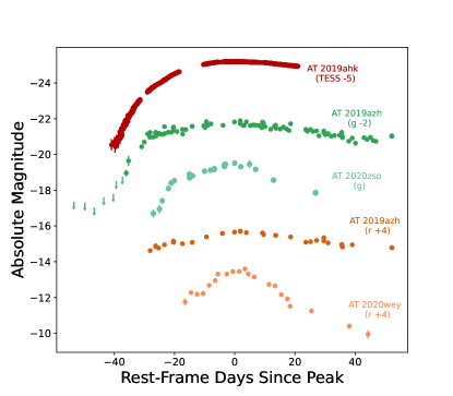
Figure 11: Comparison between the light curves of AT 2019azh (ASAS-SN and Las Cumbres data only, shown for clarity) to those of AT 2019ahk, the TDE with the most densely-sampled light curve to date (Holoien et al., 2019b), AT 2020wey (Charalampopoulos et al., 2023), and AT 2020zso. AT 2019ahk lacks any pronounced early-time light-curve structure like that seen in AT 2019azh, despite having high-cadence TESS observations. In contrast, the light curve of the TDE AT 2020wey shows a possible early “bump” in its $r$-band light curve, and AT 2020zso exhi its a change in its rising slope. Arrows indicate 3$\sigma$ nondetection upper limits.

AT 2020wey, on the other hand, is a “classical” spectroscopically classified TDE (Figure 10) which does show a possible “bump” in its early $g$- and $r$-band light curves (Figure 11; Charalampopoulos et al., 2023). Unfortunately, this part of the light curve of AT 2020wey was not observed at a sufficiently high cadence to robustly characterize this feature. Finally, AT 2020zso is a TDE which shows an abrupt change in its light-curve rise slope (Figure 11; photometry taken from Wevers et al., 2022).

No TDE emission model predicts specific light-curve features such as these; however, they might be evidence for transitions between dominant emission mechanisms. This could point toward a combination of the two proposed mechanisms (reprocessing of X-rays from the accretion disk and debris stream collisions) as responsible for the UV/optical TDE emission. The photometry presented here could be used to test future TDE emission models.

4.4 Estimates of the SMBH Mass

Wevers (2020) derived the SMBH mass of the host of AT 2019azh using the $M$–$\sigma$ relation from Gültekin et al. (2009a) with the velocity dispersion measured from the WHT spectrum presented here. They find an SMBH mass of $M_{\rm BH}=2.29\pm 2.27\times 10^{6}\,\textrm{\,M}_{\odot}$. This mass is consistent with that found by TDEMass but is a factor of $\sim 7$ smaller than that found by MOSFiT. We do not consider this definitive evidence favoring one model or the other since the host-galaxy-derived SMBH mass strongly depends on the choice of scaling relation and the spectral resolution used to infer the velocity dispersion, as is evident in the comparison to other works.

We present a summary of SMBH mass estimates obtained here and in other works using the two light-curve models and host-galaxy scaling relations, along with the corresponding Eddington ratios for the peak bolometric luminosity, in Table 7. Our results are consistent with those of Hammerstein et al. (2023) for the TDEMass estimates, and marginally consistent (at the $\lesssim 2\sigma$ level) with the MOSFiT estimates from that work. Our results are not consistent with those of Hinkle et al. (2021a) or Nicholl et al. (2022). The discrepancy with Hinkle et al. (2021a) could be due to their use of the pre-corrected UVOT calibrations introduced later by Hinkle et al. (2021b).

Table 7: SMBH mass estimates and corresponding Eddington ratios for the peak bolometric luminosity.

	TDEMass		MOSFiT		Host Galaxy
(lr)2-3 (lr)4-5 (lr)6-7	$M_{\rm BH}$ ($10^{6}\textrm{\,M}_{\odot}$)	$L_{\rm bol}$/$L_{\rm Edd}$	$M_{\rm BH}$ ($10^{6}\textrm{\,M}_{\odot}$)	$L_{\rm bol}$/$L_{\rm Edd}$	$M_{\rm BH}$ ($10^{6}\textrm{\,M}_{\odot}$)	$L_{\rm bol}$/$L_{\rm Edd}$
This Work	$2.50^{+0.29}_{-0.24}$	$0.78^{+0.22}_{-0.21}$	$16.22^{+0.75}_{-0.75}$	$0.12^{+0.03}_{-0.03}$	$2.29\pm 2.27$	$0.85\pm 0.87$
Hammerstein et al. (2023)	$2.19^{+0.14}_{-0.00}$	$0.85^{+0.18}_{-0.03}$	$26.91^{+6.81}_{-5.30}$	$0.07^{+0.02}_{-0.02}$	$-$	$-$
Hinkle et al. (2021a)	$0.73^{+0.24}_{-0.10}$	$6.75^{+2.23}_{-0.95}$	$7.8^{+3.9}_{-4.1}$	$0.63^{+0.32}_{-0.33}$	$\sim 12.59$	$\sim 0.34$
Liu et al. (2022)	$-$	$-$	$-$	$-$	$23.0^{+13.0}_{-12.0}$	$\sim 0.06$
Nicholl et al. (2022)	$-$	$-$	$5.01^{+0.70}_{-0.81}$	$-$	$-$	$-$

Note. — Eddington ratios are calculated for each source using their respective SMBH masses and peak bolometric luminosities.

4.5 Estimates of the Disrupted Star Mass

The mass derived for the disrupted star also differs substantially between the models, with TDEMass preferring a star roughly one order of magnitude more massive than MOSFiT ($4.8^{+4}_{-2.5}\,\textrm{\,M}_{\odot}$ vs. $0.10^{+0.02}_{-0.03}\,\textrm{\,M}_{\odot}$, respectively). In addition to the different model assumptions, this difference could be driven by the MOSFiT prior of a Kroupa initial mass function. Hinkle et al. (2021a) find a similar stellar mass in their MOSFiT fit as in ours, but a much higher one in their TDEMass fit than ours. As mentioned previously, this comparison may not be entirely accurate because of the Swift calibration updates (Hinkle et al., 2021b), not available to Hinkle et al. (2021a), which could influence their bolometric luminosity calculations. Hammerstein et al. (2023) also estimated the stellar mass using these two methods. Our TDEMass-based stellar mass is consistent with their findings, while our MOSFiT-based stellar mass is not. This might be due to differences in the priors used for the efficiency parameter, which is degenerate with the stellar mass. The efficiency parameter inferred from MOSFiT in our analysis is close to the maximum limit of the prior (see Figure 12 in Appendix A). This relatively high efficiency might be additional evidence for contributions to the emission from the stream collision process.

4.6 Time Lag Between $\mbox{H}{\alpha}$ Emission and the Continuum

Our time lag of $1.35\pm{1.45}$ days between the $V$-band light curve and $\mbox{H}{\alpha}$ luminosity is inconsistent with that of Hinkle et al. (2021a) who measure a $\sim 23$ day time lag. This stems mainly from a difference between our determination of the light-curve peak and theirs. Their light-curve peak was measured at MJD $58548^{+6.30}_{-2.60}$ (roughly 17 days before ours). This peak was determined by Hinkle et al. (2021a) as the median value obtained from fitting a second-order polynomial to 10,000 realizations of bolometric light curves, generated from bolometrically-corrected ASAS-SN $g$-band data, with the bolometric corrections inferred from blackbody fits. The peak light curve time determined by Hammerstein et al. (2023) of MJD $58566^{+1.16}_{-1.75}$ is closer to ours.

5 Summary and Conclusions

AT 2019azh is an H+He-TDE and is one of the best-observed UV/optical TDEs to date, having extensive spectroscopic coverage and multiwavelength photometric coverage starting several weeks before peak brightness (Figure 1). These observations reveal the following for the first time:

1. A robust change in slope and bump in the early light curve of a TDE.

2. The early evolution of the $\mbox{H}{\alpha}$ emission line in a TDE.

Unfortunately, no models exist today that can be compared to these observational characteristics; however, they could be used to constrain future models of TDE emission sources and line formation. Relatively high cadence (1–2 days) observations of TDEs are required to test if the light-curve structure observed in AT 2019azh is a common feature of rising TDE light curves.

We detect a possible MIR excess beyond what is expected from the optical/UV blackbody at those wavelengths. This excess, detected 6.7 days after $g$-band peak, might be due to a prompt dust echo. However, we are not able to determine its origin without additional observations.

The post-peak bolometric decline of AT 2019azh is not well described by a $t^{-5/3}$ power law, or by any power law, but is better fit by an exponential. We find no significant delay between the peak of the $V$-band light curve and the $\mbox{H}{\alpha}$ luminosity in AT 2019azh.

High-cadence pre-peak observations of more TDEs will be able to determine how common the features seen here are among the TDE population. In addition, more detailed modeling of TDE emission is needed to match the quality of current TDE observations and to help constrain the emission mechanism(s) in TDEs. This is an essential step before we can use TDEs to robustly measure SMBH properties.

We thank B. Mockler for helpful advice on using MOSFiT. S.F., I.A., and L.M. acknowledge support from the European Research Council (ERC) under the European Union’s Horizon 2020 research and innovation program (grant agreement number 852097). S.F. and I.A. acknowledge further support from the Israel Science Foundation (grant number 2108/18). The Las Cumbres Observatory group is supported by NSF grants AST-1911225 and AST-1911151. P. Clark and O.G. were supported by the Science & Technology Facilities Council (grants ST/S000550/1 and ST/W001225/1]). G.L. was supported by a research grant (19054) from VILLUM FONDEN. M.N. is supported by the ERC under the European Union’s Horizon 2020 research and innovation programme (grant agreement number 948381) and by UK Space Agency Grant number ST/Y000692/1. C.P.G. acknowledges financial support from the Secretary of Universities and Research (Government of Catalonia) and by the Horizon 2020 Research and Innovation Programme of the European Union under the Marie Skłodowska-Curie program. The SNICE research group acknowledges financial support from the Spanish Ministerio de Ciencia e Innovación (MCIN), the Agencia Estatal de Investigación (AEI) 10.13039/501100011033, and the European Social Fund (ESF) “Investing in your future” under the 2019 Ramón y Cajal program RYC2019-027683-I and the PID2020-115253GA-I00 HOSTFLOWS project, from Centro Superior de Investigaciones Científicas (CSIC) under the PIE project 20215AT016, and the program Unidad de Excelencia María de Maeztu CEX2020-001058-M, and from the Departament de Recerca i Universitats de la Generalitat de Catalunya through the 2021-SGR-01270 grant. S.M. and T.R. acknowledge support from the Research Council of Finland project 350458. A.V.F.’s group at UC Berkeley has been supported by the Christopher R. Redlich Fund, Briggs and Kathleen Wood (T.G.B. is a Wood Specialist in Astronomy), and numerous other donors. F.O. acknowledges support from MIUR, PRIN 2020 (grant 2020KB33TP) “Multimessenger astronomy in the Einstein Telescope Era (METE).” P. Charalampopoulos acknowledges support via an Academy of Finland grant (340613; PI R. Kotak). This work was funded in part by ANID, Millennium Science Initiative, ICN12_009.

This work is based in part on observations collected at the Las Cumbres Observatory, the Copernico 1.82 m Telescope (Asiago Mount Ekar, Italy) operated by the Italian National Astrophysical Institute – INAF, Osservatorio Astronomico di Padova, the European Organisation for Astronomical Research in the Southern Hemisphere, Chile, as part of ePESSTO under ESO program ID 199.D-0143(T) (PIs S. Smartt, C. Inserra), the Nordic Optical Telescope, owned in collaboration by the University of Turku and Aarhus University, and operated jointly by Aarhus University, the University of Turku, and the University of Oslo, representing Denmark, Finland, and Norway, the University of Iceland and Stockholm University at the Observatorio del Roque de los Muchachos, La Palma, Spain, of the Instituto de Astrofisica de Canarias, and on observations made under programme W/2019B/P7 with the William Herschel Telescope operated on the island of La Palma by the Isaac Newton Group of Telescopes in the Spanish Observatorio del Roque de los Muchachos of the Instituto de Astrofísica de Canarias. The NOT observations were obtained through the NUTS collaboration supported in part by the Instrument Centre for Danish Astrophysics (IDA). A major upgrade of the Kast spectrograph on the Shane 3 m telescope at Lick Observatory was made possible through generous gifts from William and Marina Kast as well as the Heising-Simons Foundation. Research at Lick Observatory is partially supported by a generous gift from Google. We thank for their assistance the staffs at the various observatories where data were obtained.

This research has made use of the NASA/IPAC Infrared Science Archive, which is funded by the National Aeronautics and Space Administration (NASA) and operated by the California Institute of Technology. This publication also makes use of data products from NEOWISE, which is a project of the Jet Propulsion Laboratory/California Institute of Technology, funded by the Planetary Science Division of NASA. This publication makes use of data products from the Wide-field Infrared Survey Explorer, which is a joint project of the University of California, Los Angeles, and the Jet Propulsion Laboratory/California Institute of Technology, funded by NASA. For the purpose of open access, the author have applied a Creative Commons Attribution (CC BY) licence to any Author Accepted Manuscript version arising.
 
Supporting research data are available on reasonable request from the corresponding author.

Appendix A MOSFiT Best-Fit Parameters

Figure 12 shows the two-dimensional MOSFiT posterior parameters distributions. The model fit can be seen to be well converged.

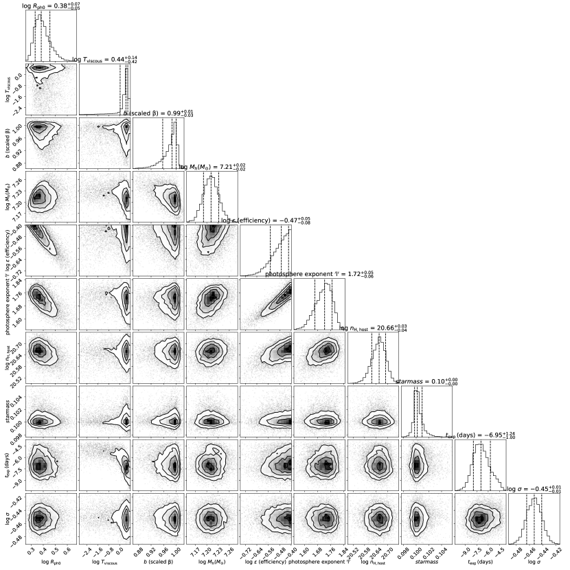
Figure 12: Corner plot showing the posterior parameter distributions for the MOSFiT model fit. 1$\sigma$ confidence intervals are marked.

Appendix B TDEMass Parameters

Figure 13 shows the inferred SMBH and star masses from TDEMass, based on the peak bolometric luminosity and the blackbody temperature at peak from SuperBol.

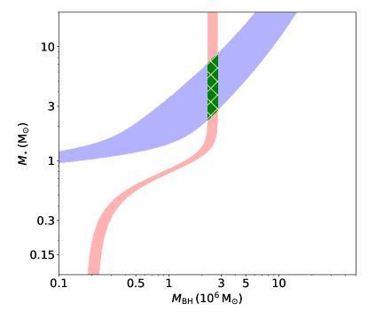
Figure 13: Inferred BH and star masses from TDEMass, with the blue shaded region indicating the range of solutions for the peak bolometric luminosity, and the red shaded region indicating the range of solutions for the blackbody temperature at this peak. The green region indicates the overlapping solutions.

Appendix C Spectral Data Processing

Figure 14 displays the step-by-step data-processing procedure applied on a spectrum obtained 14 days after the light-curve peak, as outlined in Section 3. The same procedure is applied to all spectra of AT 2019azh, apart from the duPont and the WHT spectra for the reasons detailed in Section 3.

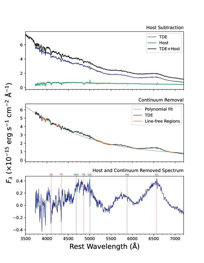
Figure 14: Top: Archival resampled SDSS host-galaxy spectrum (green), the photometrically-calibrated spectrum of AT 2019azh including host contamination, 14 days after light-curve peak (black), and the host-subtracted TDE spectrum (blue). Middle: Host-subtracted spectrum (black) with selected line-free regions (red) used for polynomial fitting (green). Bottom: Host and continuum-subtracted spectrum, showing broad $\mbox{H}{\alpha}$, He II $\lambda$4686, and He I $\lambda$5876 emission lines. The narrow [O III] $\lambda$5007 and Balmer lines are likely oversubtracted host-galaxy lines.

Figure 15 shows the spectroscopic evolution of AT 2019azh, after photometric calibration, host subtraction, and continuum removal, as described in Section 3.

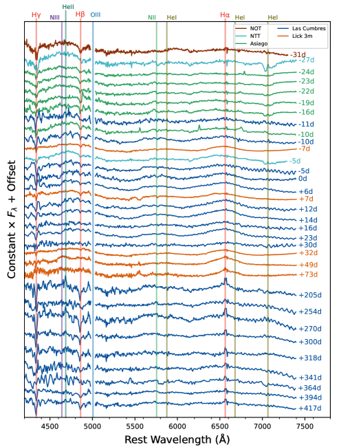
Figure 15: Spectroscopic evolution of AT 2019azh after host galaxy and continuum removal. [O III] $\lambda$5007 lines are masked for display purposes. The phase of each spectrum relative to the $g$-band light-curve peak is indicated beside it.

Figure 16 shows the Gaussian fits of the $\mbox{H}{\alpha}$ line performed on the host-galaxy and continuum-subtracted spectra.

Figure 16: Best-fit results from fitting the $\mbox{H}{\alpha}$ line with a Gaussian are shown with solid green lines and the 3$\sigma$ errors are represented in gray. In each case the dashed line indicates the initial guess for the fit. Phases are noted relative to the $g$-band light-curve peak.

References

- Abolfathi et al. (2018) Abolfathi, B., Aguado, D. S., Aguilar, G., et al. 2018, ApJS, 235, 42, doi: 10.3847/1538-4365/aa9e8a
- Alard (2000) Alard, C. 2000, A&AS, 144, 363, doi: 10.1051/aas:2000214
- Alard & Lupton (1998) Alard, C., & Lupton, R. H. 1998, ApJ, 503, 325, doi: 10.1086/305984
- Alexander et al. (2016) Alexander, K. D., Berger, E., Guillochon, J., Zauderer, B. A., & Williams, P. K. G. 2016, ApJ, 819, L25, doi: 10.3847/2041-8205/819/2/L25
- Almeida et al. (2023) Almeida, A., Anderson, S. F., Argudo-Fernández, M., et al. 2023, ApJS, 267, 44, doi: 10.3847/1538-4365/acda98
- Arcavi (2022) Arcavi, I. 2022, ApJ, 937, 75, doi: 10.3847/1538-4357/ac90c0
- Arcavi et al. (2014) Arcavi, I., Gal-Yam, A., Sullivan, M., et al. 2014, ApJ, 793, 38, doi: 10.1088/0004-637X/793/1/38
- Bade et al. (1996) Bade, N., Komossa, S., & Dahlem, M. 1996, A&A, 309, L35
- Baldwin et al. (1981) Baldwin, J. A., Phillips, M. M., & Terlevich, R. 1981, PASP, 93, 5, doi: 10.1086/130766
- Barbarino et al. (2019) Barbarino, C., Carracedo, A. S., Tartaglia, L., & Yaron, O. 2019, Transient Name Server Classification Report, 2019-287, 1
- Becker (2015) Becker, A. 2015, HOTPANTS: High Order Transform of PSF ANd Template Subtraction, Astrophysics Source Code Library, record ascl:1504.004. http://ascl.net/1504.004
- Bellm et al. (2019) Bellm, E. C., Kulkarni, S. R., Graham, M. J., et al. 2019, PASP, 131, 018002, doi: 10.1088/1538-3873/aaecbe
- Bennett et al. (2014) Bennett, C. L., Larson, D., Weiland, J. L., & Hinshaw, G. 2014, ApJ, 794, 135, doi: 10.1088/0004-637X/794/2/135
- Blagorodnova et al. (2017) Blagorodnova, N., Gezari, S., Hung, T., et al. 2017, ApJ, 844, 46, doi: 10.3847/1538-4357/aa7579
- Bogdanović et al. (2004) Bogdanović, T., Eracleous, M., Mahadevan, S., Sigurdsson, S., & Laguna, P. 2004, ApJ, 610, 707, doi: 10.1086/421758
- Bowen (1934) Bowen, I. S. 1934, PASP, 46, 146, doi: 10.1086/124435
- Bowen & Vaughan (1973) Bowen, I. S., & Vaughan, A. H. 1973, Appl. Opt., 12, 1430, doi: 10.1364/AO.12.001430
- Brown et al. (2017) Brown, J. S., Holoien, T. W. S., Auchettl, K., et al. 2017, MNRAS, 466, 4904, doi: 10.1093/mnras/stx033
- Brown et al. (2013) Brown, T. M., Baliber, N., Bianco, F. B., et al. 2013, PASP, 125, 1031, doi: 10.1086/673168
- Bu et al. (2023) Bu, D.-F., Chen, L., Mou, G., Qiao, E., & Yang, X.-H. 2023, MNRAS, 521, 4180, doi: 10.1093/mnras/stad804
- Buzzoni et al. (1984) Buzzoni, B., Delabre, B., Dekker, H., et al. 1984, The Messenger, 38, 9
- Cackett et al. (2007) Cackett, E. M., Horne, K., & Winkler, H. 2007, MNRAS, 380, 669, doi: 10.1111/j.1365-2966.2007.12098.x
- Cappelluti et al. (2009) Cappelluti, N., Ajello, M., Rebusco, P., et al. 2009, A&A, 495, L9, doi: 10.1051/0004-6361/200811479
- Cardelli et al. (1989) Cardelli, J. A., Clayton, G. C., & Mathis, J. S. 1989, ApJ, 345, 245, doi: 10.1086/167900
- Cendes et al. (2022) Cendes, Y., Berger, E., Alexander, K. D., et al. 2022, ApJ, 938, 28, doi: 10.3847/1538-4357/ac88d0