Novel class discovery meets foundation models for 3D semantic segmentation

Abstract

The task of Novel Class Discovery (NCD) in semantic segmentation entails training a model able to accurately segment unlabelled (novel) classes, relying on the available supervision from annotated (base) classes. Although extensively investigated in 2D image data, the extension of the NCD task to the domain of 3D point clouds represents a pioneering effort, characterized by assumptions and challenges that are not present in the 2D case. This paper represents an advancement in the analysis of point cloud data in four directions. Firstly, it introduces the novel task of NCD for point cloud semantic segmentation. Secondly, it demonstrates that directly transposing the only existing NCD method for 2D image semantic segmentation to 3D data yields suboptimal results. Thirdly, a new NCD approach based on online clustering, uncertainty estimation, and semantic distillation is presented. Lastly, a novel evaluation protocol is proposed to rigorously assess the performance of NCD in point cloud semantic segmentation. Through comprehensive evaluations on the SemanticKITTI, SemanticPOSS, and S3DIS datasets, the paper demonstrates substantial superiority of the proposed method over the considered baselines.

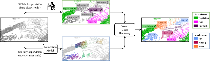
Figure 1: SNOPS addresses the novel class discovery task in 3D point cloud semantic segmentation by leveraging the knowledge of ground-truth labels (for base classes) and the auxiliary supervision from a foundation model (for novel classes) to learn the correct semantic segmentation of both base and novel points.

1 Introduction

Humans possess a remarkable ability to categorise new information (or novelties) into homogeneous groups, even when they are unfamiliar with what is observed. In contrast, machines can hardly achieve this without guidance. The primary challenges of machine vision lie in crafting discriminative latent representations of the real world and in quantifying uncertainty when faced with novelties [23, 78, 77]. [23] pioneered the formulation of the Novel Class Discovery (NCD) problem. They defined it as the endeavor to categorise samples from an unlabeled dataset, termed novel samples, into distinct classes by leveraging the insights from a set of labeled samples, known as the base samples. Note that the classes in the labeled and unlabeled datasets are disjoint.

NCD has been explored in the 2D image domain for classification [23, 16, 78] and subsequently for semantic segmentation [77]. Specifically, [77] introduced the first approach to deal with NCD in the 2D semantic segmentation task. The authors made two key assumptions. Firstly, only one novel class exists in each image. Secondly, the new class corresponds to a foreground object that is detectable through saliency detection (e.g. a man on a bicycle, with the bicycle being the novel class). Owing to these assumptions, the authors can pool the features of each image into a singular latent representation and group the representations of the entire dataset to discern clusters of novel classes. We argue that these assumptions represent significant constraints, which are difficult to satisfy with generic 3D data, especially point clouds obtained from LiDAR sensors in large-scale settings. A single point cloud may encompass multiple novel classes. Moreover, the concept of saliency for 3D data cannot be directly translated from its 2D counterpart. Although both relate to where humans direct their gaze, 3D saliency pertains more to the regional significance of 3D surfaces rather than a straightforward foreground/background distinction [56].

Our previous work, NOvel Point Segmentation (NOPS) [48] pioneers in NCD for 3D semantic segmentation, with the primary focus on addressing the above discussed limitations. NOPS has shown promising performance in tackling 3D NCD, yet, the recent emergence of 3D foundation models [40] offers us new opportunities in terms of the methodology design in NCD for their strong performance in zero-shot recognition. However we empirically show that the accuracy of using the foundation model alone in a zero-shot manner for the NCD task is significantly lower than combining it with method that is specifically designed for NCD on multiple benchmark datasets [6, 38, 3], as shown in Tables 4-6.

In this work, we present Semantically-aligned NOvel Point Segmentation (SNOPS), a method that extends NOPS [48] by making use of an additional unsupervised source of semantic knowledge, in the form of a foundation model (Fig. 1). In SNOPS, given a partially human-annotated dataset, we concurrently learn base and novel semantic classes by clustering unlabelled points based on their semantic similarities. We have adapted the methodology of [77], termed Entropy-based Uncertainty Modelling and Self-training (EUMS), to suit point cloud data, establishing it as our baseline. We advance beyond their framework and, drawing inspiration from [7] and [40], incorporate batch-level (online) clustering and distillation from foundation model into our method. The former is key to handle the large cardinality typical of 3D point cloud data, while the latter is key to leverage the intrinsic semantic knowledge contained in foundation models, such as CLIP [47]. We also modify prototypes during training to ensure computational tractability of the clustering process. The resulting cluster assignments serve as training pseudo-labels. We employ over-clustering to achieve precision that is akin to EUMS. Given the multifaceted semantic classes within point clouds, it is inevitable that not all classes are represented in every batch, leading to some omissions. To mitigate this issue, we have devised a queuing approach to retain vital features throughout the training process. These features act as a proxy for missing categories during the pseudo-labels generation, allowing for a more balanced clustering of the novel classes. We introduce a strategy that leverages pseudo-label uncertainty. This strategy aids in fostering reliable prototypes, which we subsequently harness to generate enhanced pseudo-labels. We then generate two augmented perspectives of a singular point cloud and enforce consistency in pseudo-labels between them. Our methodology is assessed on SemanticKITTI [6, 18, 5], SemanticPOSS [38], and S3DIS [3]. We establish an evaluation protocol for NCD and point cloud segmentation, serving as a potential benchmark for subsequent research. Empirical evidence suggests that our method significantly surpasses our baseline and predecessor version of our method [48] across all datasets. Additionally, we undertake a comprehensive ablation study to underscore the significance of our method’s diverse components.

To summarise, our contributions are:

• We tackle NCD for 3D semantic segmentation, addressing unfit assumptions that are originally imposed on NCD for 2D semantic segmentation;

• We provide empirical proof that zero-shot semantic segmentation with 3D foundation model is not a good enough solution for NCD.

• We present a novel method SNOPS that effectively synergises NCD method with semantic distillation through foundation model, advancing the state-of-the-art in NCD for 3D semantic segmentation;

• We introduce a new evaluation protocol to assess the performance of NCD for 3D semantic segmentation.

This paper extends our earlier work [48] in several aspects. We extend the original NOPS by leveraging a foundation model [40] to improve the accuracy of novel classes. We empirically show that the zero-shot accuracy of the foundation model alone is significantly lower than that achieved by using it in combination of our novel class discovery method. Then, we significantly extend our experimental evaluation and analysis by adding new experiments, new comparisons, and new ablation studies to evaluate this new setup. Lastly, we expand the related work by reviewing additional state-of-the-art approaches.

2 Related work

In this section, we thoroughly discuss recent works on three relevant topics, including point cloud semantic segmentation, 3D representation learning and novel class discovery.

Point cloud semantic segmentation can be performed at point level [44], on range view maps [49], or by voxelising the input points [80]. Point-level networks process the input without intermediate representations. Examples of these include PointNet [43], PointNet++ [44], RandLA-Net [25], and KPConv [59]. PointNet [43] and PointNet++ [44] are based on a series of multi-layer perceptron where PointNet++ introduces global and local feature aggregation at multiple scales. RandLA-Net [25] uses random sampling, attentive pooling, and local spatial encoding. KPConv [59] employs flexible and deformable convolutions in a continuous input space. Point-level networks are computationally inefficient when large-scale point clouds are processed. Range view architectures [36] and voxel-based approaches [12] are more computationally efficient than their point-level counterpart. The former requires projecting the input points on a 2D dense map, processing input maps with 2D convolutional filters [49], and re-projecting predictions to the initial 3D space. SqueezeSeg networks [63, 64], 3D-MiniNet [2], RangeNet++ [36], and PolarNet [75] are examples of this category. Although they are more efficient, these approaches tend to lose information during projection and re-projection. The latter includes 3D quantisation-based approaches that discretise the input points into a 3D voxel grid and employ 3D convolutions [80] or 3D sparse convolutions [21, 12] to predict per-voxel classes. VoxelNet [80], SparseConv [21, 20], MinkowskiNet [12], Cylinder3D [81], and (AF)²-S3Net [11] are architectures belonging to this category. The above-mentioned approaches usually tackle point cloud segmentation in a supervised setting, whereas we address novel class discovery with both labelled base classes and unlabelled novel classes.

3D representation learning refers to learn general and useful point cloud representations from unlabelled point cloud data [1, 66]. Existing methods can be grouped into generative, context similarity based, local descriptor based, and multi-modal approaches. Generative approaches involve the generation of a point cloud as unsupervised task [71, 70, 68]. FoldingNet [71], PSG-Net [70] and PointFlow [68] follow the autoencoder [24] paradigm and learn to self-reconstruct the input point cloud. Differently, LatentGAN [1], Tree-GAN [55] and 3D-GAN [65] follow a generative adversarial strategy and learn to generate point cloud instances from a sampled vector or a latent embedding. PU-GAN [33] and PU-GCN [45] learn the underlying geometries of point clouds by generating a denser point cloud with similar geometries. On the other hand, PCN [73], SA-Net [62], Point-BERT [72] and Point-MAE [39] learn to complete the input point cloud by predicting the arbitrary missing parts. Context similarity based approaches learn discriminative 3D representations through the underlying similarities between point samples. PointContrast [67], DepthContrast [76], ACD [17] and STRL [26] enforce the network to group feature representations through contrastive learning between positive and negative point cloud pairs. Another similarity based technique makes use of coordinate sorting as a unsupervised task. For example, Jigsaw3D [54] and Rotation3D [42] follow this idea and train the network to predict either the re-organised version or the rotation angle of the input point clouds. Local descriptor approaches focus on learning to encode per-point informative features by solving low-level tasks, e.g. point cloud registration. PPF-FoldNet [14] and CEM [30] learn compact descriptors by solving the task of point cloud matching and registration, respectively. Differently, GeDi [41] employs constrastive learning between canonical point cloud patches to learn compact and generalisable descriptors. Multi-modal approaches follow the recent success from the 2D literature [46, 15] and learn robust and comprehensive representations by modeling the relationships across modalities. Language grounding [51] maps per-point features to text CLIP [46] embeddings, providing a robust pre-training for semantic tasks. ConceptFusion [27] leverages the open-set capabilities of foundation models [22, 47, 32] from multiple modalities and fuses their features into a 3D map via traditional integration approaches. More recently, OpenScene [40] learns a feature space where text and multi-view image pixels are co-embedded in the CLIP feature space. In this work, we tackle NCD for 3D segmentation and extend our previous method NOPS [48] by leveraging the powerful representations of OpenScene [40] in our novel class discovery network.

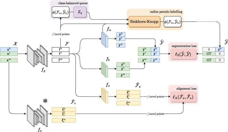
Figure 2: Overview of SNOPS. We extract point-level features $\mathcal{F}$ with the shared backbone $f_{g}$. $\mathcal{F}$ are used to obtain pseudo-labels in the online pseudo-labelling block. We forward $\mathcal{F}$ through a novel $f_{n}$ and a base $f_{b}$ segmentation head to obtain point-wise predictions. We also pass $\mathcal{F}$ through a projection layer $f_{s}$ that produces point-wise features for novel points. We align such point descriptors to the ones output by a frozen auxiliary network $f_{a}$, a large 3D vision model. The network is optimised by minimising the sum of a segmentation loss and an alignment loss.

Novel class discovery (NCD) is initially explored for 2D classification [23, 78, 16, 31, 50, 29, 79, 61, 69] and 2D segmentation [77]. NCD is formulated in a different way compared to standard semi-supervised learning [57, 74, 58]. In semi-supervised learning, labelled and unlabelled samples belong to the same classes, while in NCD, novel and base samples belong to disjoint classes. Han et al. [23] pioneered the NCD problem for 2D image classification. A classification model is pre-trained on a set of base classes and used as feature extractor for the novel classes. They then train a classifier for the novel classes using the pseudo-labels produced by the pre-trained model. Zhong et al. [78] introduced neighbourhood contrastive learning to generate discriminative representations for clustering. They retrieve and aggregate pseudo-positive pairs with contrastive learning, encouraging the model to learn more discriminative representations. Hard negatives are obtained by mixing labelled and unlabelled samples in the feature space. UNO [16] unifies the two previous works by using a unique classification loss function for both base and novel classes, where pseudo-labels are processed together with ground-truth labels. NCD without Forgetting [31] and FRoST [50] further extend NCD to the incremental learning setting. EUMS [77] is the only approach analysing NCD for 2D semantic segmentation. Unlike image classification, the model has to classify each pixel and handle multiple classes in each image. EUMS consists of a multi-stage pipeline using a saliency model to cluster the latent representations of novel classes to produce pseudo-labels. Moreover, entropy-based uncertainty and self-training are used to overcome noisy pseudo-labels while improving the model performance on the novel classes.

In this work, we focus on NCD for 3D point cloud semantic segmentation. Unlike previous works, our problem inherits the challenges from the fields of 2D semantic segmentation [10, 9] and 3D point cloud segmentation [12, 52, 36]. From 2D semantic segmentation, the main challenges are multiple novel classes in the same image and the strong class unbalance. From 3D point cloud segmentation, we have to tackle the sparsity of input data, the different density of point cloud regions and the inability to identify foreground and background, which are not present in 2D segmentation [77]. From related fields in 3D scene understanding, the previous effort REAL [8] tackles open-world 3D semantic segmentation by classifying all the unknown points into a single class. Novel classes are then labelled by a human annotator and used for learning incrementally novel classes. Instead, NOPS [48] is the first work tackling NCD for 3D semantic segmentation. Unlike [77] that uses K-Means, [48] formulate clustering as an optimal transport problem to avoid degenerate solutions, i.e. all data points may be assigned to the same label and learn a constant representation [4, 35]. On top of NOPS [48], this work incorporates the unsupervised semantic knowledge distilled from a 3D foundation model [40]. We show that the unsupervised knowledge distilled from a 3D foundation model significantly improves NCD performance.

3 Our approach

3.1 Overview

We use two UNet-like deep neural networks optimised for 3D data to extract point-level features from an input point cloud. The primary network starts untrained, serving as our target for training to concurrently segment both base and novel classes. The secondary network is auxiliary and pre-trained for task-agnostic open-vocabulary 3D scene understanding. For base class points, we use traditional supervised training, leveraging the available human annotations (ground truth). The training for novel classes pursues two distinct objectives. Firstly, we aim to align the features with the semantic knowledge of the auxiliary network (Sec. 3.6). Secondly, we adopt a self-supervised approach that generates pseudo-labels based on our online pseudo-labelling method through the the Sinkhorn-Knopp algorithm [13] (Sec. 3.3). To enable each processed batch to maintain an equal number of novel classes, even if some are absent in point clouds being processed, we use a class-balanced queue that stores features during training (Sec. 3.4). We harness the pseudo-label confidences (class probabilities) to sift out uncertain points, thus populating the queue solely with high-quality points (Sec. 3.5). Specifically, our optimisation objective is

$$\mathcal{L}=\ell_{\text{S}}+\gamma\ell_{\text{A}},$$ (1)

where $\ell_{\text{S}}$ is the segmentation loss involving ground-truth labels and pseudo-labels (Sec. 3.3), $\ell_{\text{A}}$ is the alignment loss that considers the semantic features extracted with the auxiliary network (Sec. 3.6) and $\gamma$ is a weighting factor. Fig. 2 shows the block diagram of SNOPS.

3.2 Problem formulation

Let $\mathrm{X}=\{\mathcal{X}\}$ be a dataset of 3D point clouds captured in different scenes. The point cloud $\mathcal{X}$ is a set composed of a base set $\mathcal{X}_{b}$ and a novel set $\mathcal{X}_{n}$, s.t. $\mathcal{X}=\mathcal{X}_{b}\cup\mathcal{X}_{n}$. The semantic categories that can be present in our point clouds are $\mathcal{C}=\mathcal{C}_{b}\cup\mathcal{C}_{n}$, where $\mathcal{C}_{b}$ is the set of base classes and $\mathcal{C}_{n}$ is the set of novel classes, s.t. $\mathcal{C}_{b}\cap\mathcal{C}_{n}=\emptyset$. Each $\mathcal{X}\in\mathrm{X}$ is composed of a finite but unknown number of 3D points $\mathcal{X}=\{(\mathbf{x},c)\}$, where $\mathbf{x}\in\mathbb{R}^{3}$ is the coordinate of the a point and $c$ is its semantic class. We know the class of the point $(\mathbf{x},c)$, s.t. $\mathbf{x}\in\mathcal{X}_{b}$ and $c\in\mathcal{C}_{b}$, but we do not know the class of the point $(\mathbf{x},c)$, s.t. $x\in\mathcal{X}_{n}$ and $c\in\mathcal{C}_{n}$. No points in $\mathcal{X}_{n}$ belong to one of the base classes $\mathcal{C}_{b}$. As in [23, 78, 77], we assume that the number of classes to discover is known, i.e. $|\mathcal{C}_{n}|=C_{n}$. We aim to design a computational approach that trains a deep neural network $f_{\mathbf{\Theta}}$ that can segment all the points of a given point cloud, thus learning to jointly segment base classes $\mathcal{C}_{b}$ and novel classes $\mathcal{C}_{n}$. $\mathbf{\Theta}$ are the weights of our deep neural network. $f_{\mathbf{\Theta}}$ is composed of a feature extractor network $f_{g}$, two segmentation heads $f_{n}$ and $f_{b}$ (for novel and base classes, respectively) and a feature projector $f_{s}$. $f_{\mathbf{\Theta}}=f_{g}\circ\{f_{b},f_{n},f_{s}\}$, where $\circ$ is the composition operator (Fig. 2).

3.3 Online pseudo-labelling

We formulate pseudo-labelling as the assignment of novel points to the class-prototypes learnt during training [7]. Let $\mathtt{P}\in\mathbb{R}^{D\times\rho}$ be the class prototypes, where $D$ is the size of the output features from $f_{g}$ and $\rho$ is the number of prototypes. Let $\mathtt{Z}\in\mathbb{R}^{D\times m}$ be the normalised output features extracted from $f_{g}$, i.e. $\mathtt{Z}=f_{g}(\mathcal{X})$, where $m$ is the number of points of the point cloud. $m$ is unknown a priori and it can differ across point clouds. We define $\mathtt{Q}\in\mathbb{R}^{\rho\times m}$ as the assignment between the $\rho$ prototypes and the $m$ points that equally partitions the points in the batch across the available prototypes. This equipartition ensures that the feature representations of the points belonging to different novel classes are well-separated, thus preventing the case in which the novel class feature representations collapse into a unique solution. [7] employs an arbitrary large number of prototypes $\rho$ to effectively organise the feature space produced by $f_{g}$. They discard $\mathtt{P}$ after training. In contrast, we learn exactly $\rho=C_{n}$ class prototypes and use $\mathtt{P}$ as the weights for our new class segmentation head $f_{n}$, which outputs the $C_{n}$ logits for the new classes. In order to optimise the assignment $\mathtt{Q}$, we maximise the similarity between the features of the new points and the learnt prototypes as

$$\max_{\mathtt{Q}\in\mathcal{Q}}\,\,\text{Tr}(\mathtt{Q}^{\top}\mathtt{P}^{\top}\mathtt{Z})+\epsilon H(\mathtt{Q})\rightarrow\mathtt{Q}^{*},$$ (2)

where $H$ is the entropy function, $\epsilon$ is the parameter that determines the smoothness of the assignment and $\mathtt{Q}^{*}$ is our sought solution. [4] enforce the equipartioning constraint by requiring $\mathtt{Q}$ to belong to a transportation polytope and perform this optimisation on the whole dataset at once (offline). This operation with point cloud data is computationally impractical. Therefore, we formulate the transportation polytope such that the optimisation is performed online, which consist of considering only the points within the batch being processed

$$\mathcal{Q}=\left\{\mathtt{Q}\in\mathbb{R}^{C_{n}\times m}_{+}|\mathtt{Q}\mathtt{1}_{m}=\frac{1}{C_{n}}\mathtt{1}_{C_{n}},\mathtt{Q}^{\top}\mathtt{1}_{C_{n}}=\frac{1}{m}\mathtt{1}_{m}\right\},$$ (3)

where $\mathtt{1}_{\star}$ represents a vector of ones of dimension $\star$. These constraints ensure that each class prototype is selected on average at least $m/C_{n}$ times in each batch. The solution $\mathtt{Q}^{*}$ can take the form of a normalised exponential matrix

$$\mathtt{Q}^{*}=\text{diag}(\alpha)\exp\left({\frac{\mathtt{P}^{\top}\mathtt{Z}}{\epsilon}}\right)\text{diag}(\beta),$$ (4)

where $\alpha$ and $\beta$ are renormalisation vectors that are computed iteratively with the Sinkhorn-Knopp algorithm [13, 34]. We then transpose the optimised soft assignment $\mathtt{Q}^{*}\in\mathbb{R}^{C_{n}\times m}_{+}$ to obtain the soft pseudo-labels for each of the $m$ novel points being processed within each batch.

We empirically found that training can be more effective if pseudo-labels are smoother in the first training epochs and peaked in the last training epochs. Therefore, we introduce a linear decay of $\epsilon$ during training.

Segmentation objective: The segmentation objective $\ell_{\text{S}}$ is formulated as the weighted Cross Entropy loss and it is based on the ground-truth labels $\mathcal{Y}_{b}$ for base points and on the pseudo-labels $\tilde{\mathcal{Y}}_{n}$ for novel points. We formulate a swapped prediction task based on these pseudo-labels [7]. We begin by generating two different augmentations of the original point cloud $\mathcal{X}$ that we define as $\mathcal{X}^{\prime}$ and $\mathcal{X}^{\prime\prime}$ (Fig. 3). For the augmentation $\mathcal{X}^{\prime}$ we define the segmentation predictions $\hat{\mathcal{Y}}^{\prime}=f_{b}(f_{g}(\mathcal{X^{\prime}}))\oplus f_{n}(f_{g}(\mathcal{X^{\prime}}))$, where $\oplus$ is the concatenation operator. Analogously, we define $\hat{\mathcal{Y}}^{\prime\prime}$ as the network output for $\mathcal{X}^{\prime\prime}$. The segmentation targets are defined as $\tilde{\mathcal{Y}}^{\prime}=\tilde{\mathcal{Y}}^{\prime}_{n}\cup\mathcal{Y}^{\prime}_{b}$, where $\tilde{\mathcal{Y}}^{\prime}_{n}$ are the pseudo-labels predicted with our approach and $\mathcal{Y}^{\prime}_{b}$ are the available targets for base classes (same for $\tilde{\mathcal{Y}}_{n}^{\prime\prime}$).
At this point, we enforce prediction consistency between the swapped pseudo-labels of the two augmentations as:

$$\ell_{\text{S}}(\mathcal{X})=\ell_{\text{wCE}}(\hat{\mathcal{Y}}^{\prime},\tilde{\mathcal{Y}}^{\prime\prime})+\ell_{\text{wCE}}(\hat{\mathcal{Y}}^{\prime\prime},\tilde{\mathcal{Y}}^{\prime}),$$ (5)

where $\ell_{\text{wCE}}$ is the weighted Cross Entropy loss. The weights of the loss for the base classes are computed based on their occurrence frequency in the training set. The weights of the loss for the novel classes are all set equally as their occurrence frequency in the dataset is unknown.

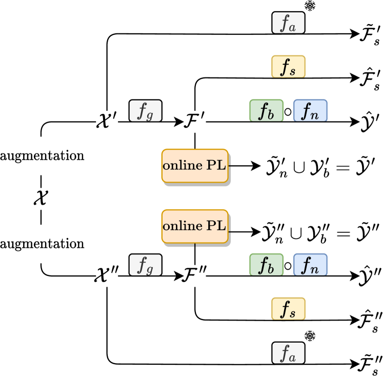
Figure 3: Overview of the different outputs after the double augmentation required for the generation of self-supervised pseudo-labels.

Multi-headed segmentation: A single segmentation head may converge to a suboptimal feature space, thus producing suboptimal prototype solutions. To further improve the segmentation quality, we use multiple novel class segmentation heads to optimise $f_{\Theta}$ based on different training solutions. Different solutions increase the likelihood of producing a diverse partitioning of the feature space as they regularise with each other (they share the same backbone) [28]. In practise, we concatenate the logits of the base class segmentation head with the outputs of each novel class segmentation head and we separately evaluate their loss for each novel class segmentation head at training time.

We task our network to over-cluster novel points, using segmentation heads that output $o\cdot C_{n}$ logits, where $o$ is the over-clustering factor. Previous studies empirically showed that this is beneficial to learn more informative features [7, 16, 35, 28]. We observed the same and concur that over-clustering can be useful for increasing expressivity of the feature representations. The over-clustering heads are then discarded at inference time.

3.4 Class-balanced queuing

Soft pseudo-labelling described in Sec. 3.3 produces an equipartite matching between the novel points and the class centroids. However, it is likely that batches are sampled with point clouds containing novel classes with different cardinalities when dealing with 3D data. It is also likely that some scenes may contain only a subset of the novel classes. Therefore, enforcing the equipartitioning constraint for each batch of the dataset could affect the learning of less frequent (long-tail) classes. As a solution, we introduce a queue $\mathtt{Z}_{q}$ containing a randomly extracted portion of the features of the novel points from the previous iterations. We use this additional data to mitigate the potential class imbalance that may occur during training. We compute $\mathtt{Z}\leftarrow\mathtt{Z}\oplus\mathtt{Z}_{q}$, where $\oplus$ is the concatenation operator, and execute the Sinkhorn-Knopp algorithm on this augmented version of $\mathtt{Z}$. The obtained $\mathtt{Q}^{*}\in\mathbb{R}^{\mathcal{C}_{n}\times(m+|\mathtt{Z}_{q}|)}$ represents the assignment between the class prototypes and all the points in the augmented version of $\mathtt{Z}$. Being interested only in the pseudo-labels for the points in the actual batch, we retain only the first $m$ columns of $\mathtt{Q}^{*}$, discarding the additional information related to the points contained in $\mathtt{Z}_{q}$.

3.5 Uncertainty-aware training and queuing

In order to build a more effective queue $\mathtt{Z}_{q}$, we select novel points for training $f_{\Theta}$ with fewer but more reliable pseudo-labels. We perform this selection by applying a threshold to the class probabilities of the novel class pseudo-labels. We found that seeking a fixed threshold for all the novel classes, that is also compatible with the variations of the class probabilities during training, is impractical. Therefore, we employ an adaptive threshold based on the class probabilities within each batch.

Our selection strategy operates as follows. Let $\tau_{c}$ be the adaptive threshold for the points of the novel class $c\in\mathcal{C}_{n}$. Firstly, we extract the novel points that have the largest class probability for the class $c$. Secondly, we compute $\tau_{c}$ as the $p$-th percentile of the class probabilities of these novel points. Lastly, we retain the novel points of class $c$ whose class probability is above the threshold $\tau_{c}$. We define this selection strategy as the function

$$\phi:(\mathcal{F}_{n},\hat{\mathcal{Y}_{n}})\times p\mapsto(\bar{\mathcal{F}}_{n}),$$ (6)

where $\mathcal{F}_{n}$ is the set of feature vectors extracted from $f_{g}$ and $\hat{\mathcal{Y}}_{n}$ is the set of class probabilities predicted by the network for these points. $\bar{\mathcal{F}}_{n}$ are both processed by the Sinkhorn-Knopp algorithm to generate our pseudo-labels and added to $\mathtt{Z}_{q}$ to make it more effective.

3.6 Incorporating semantic knowledge

The optimisation of $f_{\Theta}$ through the ground-truth labels and the pseudo-labels generated as described in Sec. 3.3 arranges the feature space output by $f_{g}$ so to effectively separate novel and base classes representations. However, the supervision provided by ground-truth targets is significantly stronger than the self-supervision of the pseudo-labels. This unbalance could result into a sub-optimal organisation of the feature space, in which base classes representations are compact and well-separated while novel classes features are instead poorly clustered, showing more noise and less compactness. To address this issue, we incorporate additional supervision for novel categories. We employ an auxiliary neural network $f_{a}$ able to output point-level semantic-aligned features, such as a 3D foundation model [40]. Such architectures have shown great performance in multiple 3D scene understanding tasks, being able to reach the results of models specifically tailored for single tasks. This high generalization capability suggests that the feature spaces of 3D foundation model are partitioned and organized according to semantics. So, by guiding our network $f_{\Theta}$ to mimic the point-level features output by $f_{a}$, we can enhance the semantical organisation of its feature space.
The most natural choice when aligning the features of our network to the ones of $f_{a}$ would be to consider the feature space output by our backbone $f_{g}$. However, there is the risk that the distillation procedure from $f_{a}$ interferes with the Sinkhorn-Knopp algorithm in organising the feature space output by $f_{g}$. So, we attach an additional projection head $f_{s}$ on top of the feature extractor $f_{g}$. The knowledge distillation from the foundation model is performed on the features $\mathcal{F}_{s}$ output by $f_{s}$, while the features $\mathcal{F}$ are kept reserved for the Sinkhorn-Knopp algorithm. A well-separated representation of novel classes in the feature space of $f_{s}$, achieved through knowledge distillation from the foundation model, can still lead to improved separation of novel classes in the feature space of $f_{g}$, since the first feature space is on top of the other and they share the same underlying architecture. The distillation procedure is performed by minimising the alignment objective:

$$\ell_{\text{A}}(\mathcal{X})=\ell_{\text{cos}}(\hat{\mathcal{F}}^{\prime}_{s},\tilde{\mathcal{F}}^{\prime}_{s})+\ell_{\text{cos}}(\hat{\mathcal{F}}^{\prime\prime}_{s},\tilde{\mathcal{F}}^{\prime\prime}_{s})$$ (7)

where $\ell_{\text{cos}}$ is the cosine loss, $\hat{\mathcal{F}}^{\prime}_{s}=f_{s}(f_{g}(\mathcal{{X}^{\prime}}))$ and $\tilde{\mathcal{F}}^{\prime}_{s}=f_{a}(\mathcal{X}^{\prime})$. The same applies for $\hat{\mathcal{F}}^{\prime\prime}_{s}$ and $\tilde{\mathcal{F}}^{\prime\prime}_{s}$ (Fig. 3). Differently from $\ell_{\text{S}}$, in this case we do not use a swapped prediction task.
The projection head $f_{s}$ and features $\mathcal{F}_{s}$ are only considered during training and we ignore this specific branch of $f_{\Theta}$ at test time.

4 Baseline methods for 3D Novel Class Discovery

SNOPS and our earlier method NOPS [48] are the first architectures proposed to tackle the task of Novel Class Discovery in point cloud semantic segmentation. So, in this work we also present two baseline methods related to 3D novel class discovery we can compare SNOPS to: the adaptation of EUMS from the image domain to the 3D point cloud domain (referred to EUMS^†) and the zero-shot testing of the OpenScene [40] model. These approaches hold significant importance in the relatively unexplored domain of 3D NCD, as they offer valuable insights into the challenges of such task. In particular, EUMS^† serves as a baseline to highlight the challenges in naively adapting 2D methods to the 3D domain. The zero-shot testing with OpenScene provides instead a reference point, demonstrating the deep scene understanding capabilities of 3D Vision-Language Models and highlighting also the difficulties encountered in their application.

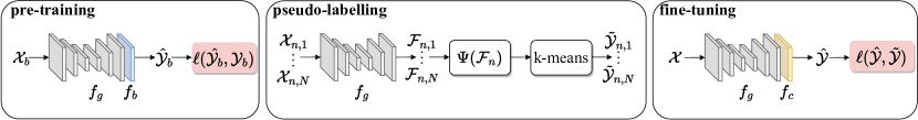
Figure 4: Overview of EUMS^†, our adaptation of the method proposed by [77]. We first pre-train $f_{g}$ and $f_{b}$ considering only the base points in each point cloud. Using $f_{g}$, we extract the features of the novel points in each scene, that are filtered with the selection function $\Psi(\cdot)$. Then, we produce the pseudo-labels for the selected novel points by using the k-means algorithm. Lastly, we plug a new segmentation head $f_{c}$ into $f_{g}$ and fine-tune the complete model on both novel and base points, considering pseudo-labels and ground-truth labels respectively.

4.1 Adapting NCD for 2D images to 3D point clouds

One of the contributions of this work is to adapt the method proposed by [77] for NCD in 2D semantic segmentation (EUMS) to 3D data. Our empirical evaluation (see Sec. 5) shows that the transposition of EUMS to the 3D domain has some limitations. In particular, as described in Sec. 1, EUMS uses two assumptions: I) the novel classes belong to the foreground and II) each image can contain at most one novel class. This allows EUMS to leverage a saliency detection model to produce a foreground mask and a segmentation model pre-trained on the base classes to determine which portion of the image is background. The portion of the image that belongs to both the foreground mask and the background mask is where features are then pooled. EUMS computes a feature representation for each image by average pooling the features of the pixels belonging the unknown portion. The feature representations of all the images in the dataset are clustered with K-Means by using the number of classes to discover as the target number of clusters. EUMS shows that overclustering and entropy-based modelling can be exploited to improve the results. The affiliation of a point to its cluster is used to produce hard pseudo-labels that are in turn used along with the ground-truth labels to fine-tune the pre-trained model.

With 3D point clouds, there is no concept of foreground and background (in contrast with I). Our adaptation is designed to discover the classes of all the unlabelled points (in contrast with II). Therefore, given the unlabelled points of each point cloud, we randomly extract a subset of these by setting a ratio (e.g. 30%) with upper bound (e.g. 1K) on the number of points to select. We compute and collect their features for all the point clouds in the dataset and apply K-Means on the whole set of features. Note that this clustering step is computationally expensive, and we had to use High Performance Computing to execute it. The subsampling of the points was necessary to fit the data in the RAM (see Sec. 5 for a detailed analysis). Once the cluster prototypes are computed, we produce the hard pseudo-labels. To enrich the set of pseudo-labels, we propagate the pseudo-label of each point to its nearest neighbour in the coordinate space. This allows us to expand the subset of pseudo-labelled randomly selected points. We also implement the other steps of overclustering and entropy-based modelling to boost the results. Lastly, we fine-tune our model with these pseudo-labels. We name our transposition of EUMS as EUMS^† and report its block diagram in Fig. 4.

4.2 Zero-shot testing with OpenScene

3D Vision-Language Models (3D-VLMs) have shown promising generalization capabilities in scene understanding  [40], especially in the context of 3D semantic segmentation. Their capabilities can be used off-the-shelf to recognize new objects within scenes by providing the correct text prompt. In this section, we assess the zero-shot semantic segmentation capabilities of the OpenScene models [40]. Our objective is to evaluate these 3D-VLMs on datasets that differ from the ones they were distilled from. We consider this testing to be our lower bound and with SNOPS we aim to improve over it.
We report in Fig. 5 the implementation of our zero-shot experiment. The input point cloud $\mathcal{X}$ is forwarded into the frozen $f_{\text{vision}}$, resulting in point-wise CLIP-aligned features $\mathcal{F}_{\text{v}}$. Subsequently, the frozen text encoder $f_{\text{text}}$ is provided with classical prompts following the template An image of a <CLASS> for all the classes present in the dataset. This process yields the output $\mathcal{F}_{\text{t}}$. Finally, we use the pairwise cosine similarity between each point and class name embedding to assign the predicted classes $\hat{\mathcal{Y}}$.
In its naive version, this experiment would imply the use of dataset class names as input prompts with a simple text template,e.g., An image of a <CLASS>. However, we argue that the simple use of the given dataset class names may limit zero-shot capabilities of OpenScene. Dataset names are selected from a (large) set of synonyms with the same meaning, e.g., person can also be indicated with the words pedestrian or walker. Oppositely, the CLIP text encoder has been trained with descriptors that contain different terms for the same concept and consequently it has learnt slightly different embeddings for each of the synonyms of the same concept. So, deriving a single text embedding for each class (e.g. for the dataset class name person) does not ensure the coverage of all the variations inside such class (e.g. for walker and pedestrian). To this extent, we propose to map each class name to four additional synonyms, which capture different meanings under the same class name. Similarly to what proposed for the text templates, we use the five different embeddings for each class as an ensemble. This enable a better coverage ot the CLIP feature space and increases the zero-shot capabilities of OpenScene. The synonyms for each class are extracted by querying the WordNet dataset [37]. When the returned words are not enough, we also make use of Thesaurus.com for additional synonyms.To further exploit the sensitivity of $f_{text}$ to text input [47], we use an ensemble of text templates to produce robust and stable predictions. In particular, we use the 80 templates originally proposed in [47].
Tab. 4, 5 & 6 show the OpenScene zero-shot performance on SemanticPOSS, SemanticKITTI, and S3DIS respectively. On SemanticPOSS, our method using ensembles of 3 synonyms reaches $21.18\%$ mIoU, surpassing the standard testing with single class words by around $2.4\%$. The testing with 5 synonyms shows even better results, showing an overall $23.05\%$ mIoU, with an improvement over the baseline of around $4.3\%$. On SemanticKITTI, we reach $19.28\%$ mIoU with 5 synonyms, improving over the testing with 3 synonyms by around $0.7\%$ and gaining $1.0\%$ mIoU over the standard testing with single class words. On S3DIS, we report the results without using ensembles of synonyms, since the furniture class names (e.g. chair) of this dataset are too specific to find suitable synonyms for each class label. The zero-shot testing of OpenScene on the S3DIS dataset results in an overall 36.76 mIoU.

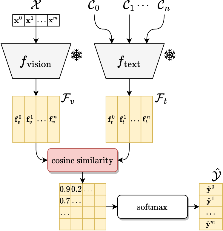
Figure 5: Zero-shot 3D semantic segmentation. We extract point-level features from the 3D vision encoder $f_{vision}$ and text embedding from the text encoder $f_{text}$. We assume class vocabularies to be known. Class predictions are assigned by similarity matching between point-level features and text embedding.

5 Experimental results

5.1 Experiments

Datasets. We evaluate our approach on SemanticKITTI [6, 18, 5], SemanticPOSS [38], and Stanford 3D Indoor Scene Dataset (S3DIS) [3]. SemanticKITTI [6] consists of 43,552 point cloud acquisitions with point-level annotations of 19 semantic classes. Based on the conventional benchmark guidelines [6], we use sequence $08$ for validation and the other sequences for training. SemanticPOSS [38] consists of 2,988 real-world point cloud acquisitions with point-level annotations of 13 semantic classes. Based on the conventional benchmark guidelines [38], we use sequence $03$ for validation and the other sequences for training. S3DIS [3] consists of 271 indoor RGB-D scans with point-level annotations of 13 semantic classes. We follow the official split [3] and use Area_5 for validation and the other areas for training.

Experimental protocol for 3D NCD. Similarly to what proposed by [77] in the 2D domain, we create different splits of each dataset to validate the NCD performance with point cloud data. We create four splits for SemanticKITTI, SemanticPOSS and S3DIS. We refer to these splits as SemanticKITTI-$n^{i}$, SemanticPOSS-$n^{i}$ and S3DIS-$n^{i}$, where $i$ indexes the split. In each set, the novel classes and the base classes correspond to unlabelled and labelled points, respectively. Tabs. 1, 2 & 3 detail the splits of our datasets. These splits are selected based on their class distribution in the dataset and on the semantic relationship between novel and base classes, e.g. in KITTI-$4^{3}$ the base class motorcycle can be helpful to discover the novel class motorcyclist.

Table 1: SemanticKITTI splits, is defined as KITTI-$n^{i}$, where $n$ is the number of novel classes and $i$ is the split index.

Split	Novel Classes
KITTI-$5^{0}$	building, road, sidewalk, terrain, veget.
KITTI-$5^{1}$	car, fence, other-ground, parking, trunk
KITTI-$5^{2}$	motorc., other-v., pole, traffic-s., truck
KITTI-$4^{3}$	bicycle, bicyclist, motorcyclist, person

Table 2: SemanticPOSS splits, defined as POSS-$n^{i}$, where $n$ is the number of novel classes and $i$ is the split index.

Split	Novel Classes
POSS-$4^{0}$	building, car, ground, plants
POSS-$3^{1}$	bike, fence, person
POSS-$3^{2}$	pole, traffic-sign, trunk
POSS-$3^{3}$	cone-stone, rider, trashcan

Table 3: S3DIS splits, defined as S3DIS-$n^{i}$, where $n$ is the number of novel classes and $i$ is the split index.

Split	Novel Classes
S3DIS-$4^{0}$	ceiling, clutter, floor, wall
S3DIS-$3^{1}$	chair, door, table
S3DIS-$3^{2}$	beam, bookcase, column
S3DIS-$3^{3}$	board, sofa, window

We quantify the performance by using the mean Intersection over Union (mIoU), which is defined as the average IoU across the considered classes [6]. We provide separate mIoU values for the base and novel classes. We also report the overall mIoU computed across all the classes in the dataset for completeness.

Implementation Details. We implement our network based on a MinkowskiUNet-34C network [12]. Point-level features are extracted from the penultimate layer. The segmentation heads $f_{b}$ and $f_{n}$ are implemented as linear layers, producing output logits for each point in the batched point clouds. The projection head $f_{s}$ is a sequence of linear layer, batch norm, ReLU, and another linear layer. The auxiliary network $f_{a}$ is the MinkowskiUNet-18 network presented in OpenScene [40]. We use the version distilled from nuScenes-OpenSeg for SemanticKITTI-$n^{i}$ and SemanticPOSS-$n^{i}$, and the version distilled from ScanNet-OpenSeg for S3DIS-$n^{i}$. We train our network for 10 epochs for SemanticKITTI-$n^{i}$ and SemanticPOSS-$n^{i}$, and for 50 epochs for S3DIS-$n^{i}$. We use the SGD optimizer, with momentum 0.9 and weight decay 0.0001. Our learning rate scheduler consists of linear warm-up and cosine annealing, with $lr_{max}=10^{-2}$ and $lr_{min}=10^{-5}$. We train with batch size equal to 4. We employ five segmentation heads, that are used in synergy with an equal number of over-clustering heads, with $o=3$. In $\phi$, we set $p=0.5$ for SemanticKITTI-$n^{i}$, and $p=0.3$ for SemanticPOSS-$n^{i}$ and S3DIS. We set $\gamma=3.0$ for SemanticKITTI-$n^{i}$, and $\gamma=7.0$ for SemanticPOSS-$n^{i}$ and S3DIS. We adapted the implementation of the Sinkhorn-Knopp algorithm [13] from the code provided by [7], with the introduction of the queue and an in-place normalisation steps. Similarly to [7], we set $n_{sk\_iters}=3$, while we adopt a linear decay for $\epsilon$, with $\epsilon_{start}=0.3,\epsilon_{end}=0.05$.

Table 4: Novel class discovery results on SemanticPOSS. SNOPS outperforms EUMS^† and NOPS on all the four splits. Full supervision: model trained with labels for base and novel classes. Zero-shot: reference described in Sec. 4.2 (“n Syn” indicates the number n of synonyms used to build the ensembles). EUMS^†: baseline described in Sec. 4.1. Highlighted values are the novel classes in each split.

Split	Model	bike	build.	car	cone.	fence	grou.	pers.	plant	pole	rider	traf.	trash.	trunk	mIoU
															Novel	Base	All
	Full supervision	43.20	71.30	33.00	32.50	44.60	78.50	61.80	73.90	30.90	54.70	26.70	11.00	19.30	-	-	44.72
	Zero-shot - 1 Syn.	0.08	50.34	38.71	1.31	6.37	61.12	31.78	48.47	2.45	0.05	0.00	2.74	0.57	-	-	18.77
	Zero-shot - 3 Syn.	0.06	52.29	39.32	0.34	5.97	61.96	41.79	61.00	3.21	0.00	0.00	4.46	4.98	-	-	21.18
	Zero-shot - 5 Syn.	0.06	55.60	38.62	0.12	6.63	67.04	42.00	67.81	5.72	2.83	1.61	5.37	6.28	-	-	23.05
POSS-$4^{0}$	EUMS†[77]	25.67	3.98	0.56	16.44	29.40	36.76	43.84	28.46	13.13	26.75	18.18	3.34	16.91	17.44	21.52	20.26
	NOPS [48]	35.47	30.35	1.24	13.52	24.13	69.14	44.70	42.07	19.19	47.65	24.44	8.17	21.82	35.70	26.57	29.38
	SNOPS (Ours)	34.21	58.80	10.04	13.20	18.69	77.25	45.84	58.62	17.27	48.35	22.61	8.72	22.85	51.18	25.75	33.57
POSS-$3^{1}$	EUMS†[77]	15.17	67.98	28.02	23.98	11.88	75.07	35.98	74.46	26.91	48.56	26.00	5.60	23.05	21.01	39.96	35.59
	NOPS [48]	29.35	71.35	28.70	12.21	3.94	78.24	56.78	74.21	18.29	38.88	23.31	13.74	23.51	30.02	38.24	36.35
	SNOPS (Ours)	16.29	71.37	30.01	19.75	24.90	77.14	54.96	73.36	15.76	38.43	22.28	15.74	23.59	32.05	38.72	37.18
POSS-$3^{2}$	EUMS†[77]	40.14	69.45	27.67	13.50	34.86	76.03	54.66	75.59	5.27	39.22	7.79	8.52	11.85	8.31	43.96	35.74
	NOPS [48]	37.16	71.81	29.74	14.64	28.38	77.53	52.09	73.00	11.51	47.11	0.54	10.20	14.79	8.95	44.17	36.04
	SNOPS (Ours)	38.37	72.45	27.96	14.47	26.19	78.08	54.73	74.31	9.99	48.25	22.98	10.16	17.71	16.89	44.50	38.13
POSS-$3^{3}$	EUMS†[77]	41.17	70.68	28.08	4.34	38.27	76.66	38.29	75.35	25.76	34.34	28.31	0.36	24.40	13.01	44.70	37.38
	NOPS [48]	38.55	70.36	30.91	0.00	29.38	76.50	55.98	71.84	17.03	31.87	26.15	0.95	22.57	10.94	43.93	36.32
	SNOPS (Ours)	39.40	70.33	30.03	9.10	26.84	77.64	54.32	72.54	16.02	49.89	28.13	1.31	23.51	20.10	43.88	38.39
											Avg	EUMS†[77]			14.94	37.54	32.24
												NOPS [48]			21.40	38.23	34.52
												SNOPS (Ours)			30.05	38.21	36.82

Table 5: Novel class discovery results on SemanticKITTI. SNOPS outperforms EUMS^† and NOPS on all four splits. Full supervision: model trained with labels for base and novel classes. Zero-shot: reference described in Sec. 4.2 (“n Syn” indicates the number n of synonyms used to build the ensembles). EUMS^†: baseline described in Sec. 4.1. Highlighted values are the novel classes in each split.

Split	Model	bi.cle	b.clst	build.	car	fence	mt.cle	m.clst	oth-g.	oth-v.	park.	pers.	pole	road	sidew.	terra.	traff.	truck	trunk	veget.	mIoU
																					Novel	Base	All
	Full supervision	6.30	39.50	85.40	90.00	23.20	20.30	5.70	3.90	18.00	28.90	31.00	40.60	90.90	74.60	62.10	20.50	62.90	46.20	83.90	-	-	43.89
	Zero-shot - 1 Syn.	0.00	5.20	40.59	55.57	8.12	11.22	0.50	0.05	4.26	0.10	17.16	4.05	62.89	34.74	0.00	0.04	41.39	0.31	61.25	-	-	18.29
	Zero-shot - 3 Syn.	0.04	0.00	42.56	44.53	8.01	8.55	5.25	0.09	0.27	0.25	23.80	6.19	45.57	36.71	11.48	0.01	41.30	5.48	72.45	-	-	18.55
	Zero-shot - 5 Syn.	0.18	1.53	48.51	32.89	7.99	9.29	4.34	0.00	0.06	0.22	21.19	8.08	38.20	35.62	34.18	1.36	41.20	6.82	74.60	-	-	19.28
KITTI-$5^{0}$	EUMS†[77]	5.28	39.96	15.77	79.20	9.03	16.89	2.52	0.07	11.39	14.40	12.67	29.17	42.58	26.10	0.05	10.30	47.37	37.92	38.35	24.57	21.08	23.11
	NOPS [48]	5.59	47.76	52.68	82.60	13.76	25.55	1.36	1.66	14.52	19.80	25.86	32.12	56.74	8.08	23.84	14.28	49.41	36.18	44.17	37.10	24.70	29.62
	SNOPS (Ours)	6.64	43.88	71.95	83.34	13.63	24.74	2.47	2.40	15.12	18.67	24.61	31.60	49.47	43.15	27.36	15.68	42.12	38.52	37.46	45.88	25.96	31.20
KITTI-$5^{1}$	EUMS†[77]	7.53	42.41	79.97	76.77	8.62	19.58	1.39	0.57	12.03	14.14	13.95	40.74	86.32	66.45	56.29	11.97	44.79	20.94	72.40	24.21	37.06	35.62
	NOPS [48]	7.36	51.23	84.53	50.87	7.27	28.93	1.76	0.00	22.20	19.39	30.42	37.61	90.07	72.18	60.75	16.78	57.34	49.25	85.12	25.36	43.09	40.69
	SNOPS (Ours)	7.58	43.48	85.12	68.70	18.98	24.42	3.48	0.00	23.86	19.09	27.00	36.50	89.30	71.92	61.99	17.16	55.85	29.42	84.37	27.24	45.15	40.43
KITTI-$5^{2}$	EUMS†[77]	8.26	50.78	82.98	88.05	17.88	2.75	2.32	0.17	3.16	25.40	24.98	20.20	88.30	71.04	57.85	8.63	27.16	38.36	76.95	12.38	42.22	36.59
	NOPS [48]	6.72	49.24	86.36	90.79	23.68	2.69	0.58	1.87	15.46	29.48	27.92	36.39	90.26	73.39	61.21	17.83	10.32	46.16	84.29	16.54	44.80	39.72
	SNOPS (Ours)	6.79	48.30	86.08	89.88	22.20	9.27	0.56	3.55	10.51	28.35	27.10	23.81	90.64	73.79	61.93	22.31	22.11	46.06	83.76	17.60	47.85	39.84
KITTI-$4^{3}$	EUMS†[77]	3.95	2.47	80.10	87.21	16.81	14.02	14.98	0.31	14.13	20.77	6.80	37.59	86.79	66.50	55.26	16.20	40.62	38.37	76.15	7.05	43.39	35.74
	NOPS [48]	2.32	27.83	86.04	89.89	23.06	24.47	2.92	3.06	18.19	30.09	16.32	39.90	90.65	73.51	61.04	17.40	49.76	44.01	83.18	12.35	48.95	41.24
	SNOPS (Ours)	4.65	31.51	84.55	88.65	22.81	23.28	8.23	2.62	17.89	28.69	15.05	38.26	89.71	72.48	60.76	16.14	43.34	45.70	82.87	14.86	47.85	40.91
																Avg	EUMS†[77]				17.05	35.94	32.76
																	NOPS [48]				22.84	42.39	37.73
																	SNOPS (Ours)				26.39	41.69	38.10

Table 6: Novel class discovery results on S3DIS. SNOPS outperforms EUMS^† on all the four splits and NOPS on three out of the four splits. Full supervision: model trained with annotations for base and novel classes. Zero-shot: reference described in Sec. 4.2 (“n Syn” indicates the number n of synonyms used to build the ensembles). EUMS^†: baseline described in Sec. 4.1. Highlighted values are the novel classes in each split.

Split	Model	beam	board	book.	ceil.	chair	clutt.	col.	door	floor	sofa	table	wall	wind.	mIoU
															Novel	Base	All
	Full supervision	0.05	13.46	58.45	75.88	74.72	35.08	22.55	39.62	91.29	21.31	67.55	68.27	9.33	-	-	44.43
	Zero-shot - 1 Syn.	0.00	0.00	42.36	72.78	56.25	10.81	0.00	47.17	85.53	45.48	42.31	59.24	15.95	-	-	36.76
S3DIS-$4^{0}$	EUMS†[77]	0.02	12.15	42.27	41.65	59.30	10.08	19.85	24.29	0.23	26.99	43.50	3.56	6.03	13.88	26.04	22.30
	NOPS [48]	0.04	8.05	52.79	48.00	67.39	20.03	25.98	36.83	0.00	38.12	63.05	36.28	6.48	26.08	33.19	31.00
	SNOPS (Ours)	0.55	0.12	49.86	81.01	72.82	9.99	28.48	35.48	94.39	43.50	64.37	38.37	2.91	55.94	33.12	40.14
S3DIS-$3^{1}$	EUMS†[77]	0.17	14.06	34.90	72.63	2.67	20.11	19.70	6.74	87.56	26.05	19.66	63.58	3.66	9.69	34.24	28.58
	NOPS [48]	0.00	8.14	54.44	78.49	22.49	37.03	27.81	19.07	94.28	55.17	49.69	64.34	11.00	30.41	43.07	40.15
	SNOPS (Ours)	0.00	8.81	53.78	81.77	58.14	36.61	27.62	42.43	94.29	57.45	59.90	63.52	10.98	53.49	43.49	45.79
S3DIS-$3^{2}$	EUMS†[77]	0.03	3.90	27.36	76.43	68.21	23.99	2.18	25.07	91.55	34.68	64.51	63.55	0.99	9.86	45.29	37.11
	NOPS [48]	0.52	12.06	33.89	73.28	75.53	33.35	6.56	30.24	92.99	50.51	68.36	64.99	6.94	13.66	50.83	42.25
	SNOPS (Ours)	0.93	6.29	33.34	79.59	76.69	36.74	12.26	32.57	95.91	46.14	67.65	62.92	5.37	15.51	50.99	42.80
S3DIS-$3^{3}$	EUMS†[77]	0.02	5.32	56.68	77.26	72.70	36.71	28.52	45.24	93.64	4.41	69.21	59.09	2.52	4.08	59.91	42.41
	NOPS [48]	0.12	0.29	54.54	79.44	78.01	38.07	27.68	39.04	95.50	30.25	67.77	68.18	8.44	12.99	54.83	45.18
	SNOPS (Ours)	0.00	7.26	56.55	82.90	76.56	36.82	25.87	44.71	96.38	20.23	65.61	66.91	6.24	11.24	55.23	45.08
										Avg	EUMS†[77]				9.38	39.87	32.60
											NOPS [48]				20.79	45.48	39.65
											SNOPS (Ours)				34.05	45.71	43.45

5.2 Quantitative analysis

We evaluate SNOPS on both outdoor LiDAR datasets (SemanticPOSS [38] and SemanticKITTI [6]) and indoor RGB-D datasets (S3DIS [3]). For each setting, we report the upper bound Full supervision obtained by supervised training over both base and novel classes. We name with Zero-shot - n Syn. the zero-shot results achieved by OpenScene as described in Sec. 4.2 using n synonyms when building the ensembles. This baseline is our competitor for the performance achieved on novel classes. EUMS^† (Sec.4.1) and NOPS [48] are the NCD approaches that we directly compare against SNOPS.

Outdoor datasets. Tab. 4 and Tab. 5 report the segmentation results on SemanticPOSS and SemanticKITTI, respectively.
On SemanticPOSS, SNOPS achieves $30.05$ IoU on novel classes, improving of $+15.11$ IoU over EUMS^† and $+8.65$ IoU over NOPS (Tab. 4). SNOPS outperforms the other methods on all the four dataset splits and on all the classes, except for bike, person, and pole, where NOPS achieves better results. We attribute the significant decline in performance observed in SNOPS for the bike class to the alignment procedure with the auxiliary zero-shot model, since the auxiliary zero-shot network exhibits notably poor results on this particular class (0.06 IoU). We consider the decrease in performance for the other two classes (i.e. person and pole) as simple fluctuations that may happen when SNOPS organizes its feature space differently from the one of NOPS. SNOPS improves over the reference Zero-shot baseline of $+7.00$ IoU, outperforming it on all classes, apart for car, plant and trashcan. Interestingly, the Zero-shot setting outperforms even the Full supervision upper bound on the car class.
On SemanticKITTI, SNOPS achieves $26.39$ IoU on novel classes, improving of $+9.34$ IoU over EUMS^† and $+3.55$ IoU over NOPS (Tab. 5). SNOPS outperforms all the compared approaches on all the SemanticKITTI splits, showing a large improvement on novel classes, e.g., building and sidewalk. Again, SNOPS improves over the reference Zero-shot baseline of $+7.11$ IoU, outperforming it on 14 out of 19 classes, surpassing it with a large margin in the classes bicyclist, car, and traffic-sign. Interestingly, SNOPS outperforms the Full supervision upper bound on the traffic-sign class, with an improvement of $+1.81$ IoU.

Indoor dataset. Tab. 6 reports the results on the indoor S3DIS dataset. In this settings, SNOPS achieves $34.05$ IoU on novel classes, improving of $+24.67$ IoU over EUMS^† and $+13.26$ IoU over NOPS. SNOPS outperforms by a large margin EUMS^† on all four splits. Compared to NOPS, it improves on three out of four splits, with the remarkably large margins of $+29.86$ IoU and $+23.08$ IoU on S3DIS-$4^{0}$ and S3DIS-$3^{1}$, respectively. Considering the average performance over base and novel classes, SNOPS notably surpasses the results obtained by Full supervision on two out of four splits (S3DIS-$3^{1}$ and S3DIS-$3^{3}$), with $43.45$ IoU in average over the four splits (only $-0.98$ as compared to Full supervision).

\begin{overpic}[width=86.72267pt]{images/t-SNE/POSS-4_0_NOPS.png} \put(0.0,85.0){\color[rgb]{0,0,0}\footnotesize{NOPS~{}\cite[citep]{[\@@bibref{Number}{riz2023novel}{}{}]}}} \put(-10.0,30.0){\small\rotatebox{90.0}{\color[rgb]{0,0,0}\footnotesize{POSS-$4^{0}$}}} \end{overpic}	\begin{overpic}[width=86.72267pt]{images/t-SNE/POSS-4_0_NOPSv2.png} \put(25.0,85.0){\color[rgb]{0,0,0}\footnotesize{SNOPS~{}(Ours)}} \end{overpic}		\begin{overpic}[width=86.72267pt]{images/t-SNE/POSS-3_1_NOPS.png} \put(0.0,85.0){\color[rgb]{0,0,0}\footnotesize{NOPS~{}\cite[citep]{[\@@bibref{Number}{riz2023novel}{}{}]}}} \put(-10.0,30.0){\small\rotatebox{90.0}{\color[rgb]{0,0,0}\footnotesize{POSS-$3^{1}$}}} \end{overpic}	\begin{overpic}[width=86.72267pt]{images/t-SNE/POSS-3_1_NOPSv2.png} \put(25.0,85.0){\color[rgb]{0,0,0}\footnotesize{SNOPS~{}(Ours)}} \end{overpic}
\begin{overpic}[width=429.28616pt]{images/qualitative/poss/legend_poss.pdf} \end{overpic}
\begin{overpic}[width=86.72267pt]{images/t-SNE/KITTI-5_0_NOPS.png} \put(-10.0,30.0){\small\rotatebox{90.0}{\color[rgb]{0,0,0}\footnotesize{KITTI-$5^{0}$}}} \end{overpic}	\begin{overpic}[width=86.72267pt]{images/t-SNE/KITTI-5_0_NOPSv2.png} \end{overpic}		\begin{overpic}[width=86.72267pt]{images/t-SNE/KITTI-5_1_NOPS.png} \put(-10.0,30.0){\small\rotatebox{90.0}{\color[rgb]{0,0,0}\footnotesize{KITTI-$5^{1}$}}} \end{overpic}	\begin{overpic}[width=86.72267pt]{images/t-SNE/KITTI-5_1_NOPSv2.png} \end{overpic}
\begin{overpic}[width=429.28616pt]{images/qualitative/kitti/legend_kitti.pdf} \end{overpic}
\begin{overpic}[width=86.72267pt]{images/t-SNE/S3DIS-4_0_NOPS.png} \put(-10.0,30.0){\small\rotatebox{90.0}{\color[rgb]{0,0,0}\footnotesize{S3DIS-$4^{0}$}}} \end{overpic}	\begin{overpic}[width=86.72267pt]{images/t-SNE/S3DIS-4_0_NOPSv2.png} \end{overpic}		\begin{overpic}[width=86.72267pt]{images/t-SNE/S3DIS-3_1_NOPS.png} \put(-10.0,30.0){\small\rotatebox{90.0}{\color[rgb]{0,0,0}\footnotesize{S3DIS-$3^{1}$}}} \end{overpic}	\begin{overpic}[width=86.72267pt]{images/t-SNE/S3DIS-3_1_NOPSv2.png} \end{overpic}
\begin{overpic}[width=429.28616pt]{images/qualitative/s3dis/legend_s3dis.pdf} \end{overpic}

Figure 6: t-SNE dimensionality reduction of the embedding space output by the feature extractors $f_{\xi}$ of NOPS and SNOPS for the novel points in different splits of our datasets. Compared to NOPS, SNOPS is able to better organize its embedding space, better grouping features of the novel classes in more compact and separated clusters.

Discussion. SNOPS consistently outperforms the compared baselines across most of the splits within the three datasets. While the superiority of SNOPS over other NCD methods is empirically clear, understanding the underlying factors contributing to this improvement is essential. Compared to EUMS^†, SNOPS achieves superior performance, thanks to online pseudo-labelling (shared with NOPS). This enables precise refinement and adaptation of the model’s predictions and leads to better results. Compared to NOPS, SNOPS incorporates an alignment procedure that injects unsupervised semantic knowledge into our architecture. To assess the impact of the semantically-aligned branch, we compare the tSNE [60] dimensionality reduction of the embedding spaces of NOPS and SNOPS, as shown in Fig. 6. We randomly selected eight point clouds from the validation set of each dataset and processed them through the feature extractors of both NOPS and SNOPS, resulting in point-wise features. From these, we retained $5000$ random novel points along with their respective features, applied t-SNE reduction, and visualized the points with colors corresponding to their ground-truth labels. As illustrated in Fig. 6, SNOPS exhibits a more refined organization of the feature space, characterized by compact and well-separated class clusters. This contributes to the observed performance enhancement between SNOPS and NOPS. SNOPS also significantly improves over the Zero-shot baseline on two out of three datasets, highlighting that relying solely on the zero-shot capabilities of the auxiliary network is not enough for performance. In contrast, SNOPS adeptly integrates the advantages of online pseudo-labelling and semantic alignment, showcasing its ability in making these components work in synergy for superior performance in point cloud semantic segmentation.
In our opinion, the performance of the auxiliary zero-shot network fluctuates significantly based on what we deem as class representation disparities between the distillation and testing datasets; it performs relatively well for well-represented classes but it encounters substantial challenges in accurately identifying rare classes during testing.

Computational time. SNOPS shows a drastic reduction in the computational time when compared to EUMS^†. Firstly, EUMS^† requires a pre-training step and a fine-tuning step, i.e. 30 training epochs in total. Then, EUMS^† requires a large amount of memory (up to 200 GB memory for KITTI-$5^{0}$) to store the data required for clustering, taking several hours (50 hrs) to complete the training procedure. Differently, SNOPS achieves superior performance with 10 training epochs, by using less memory (10 GB max) and a lower computational time (up to 25 hrs for KITTI-$5^{0}$). We run these tests using one GPU Tesla A40-48GB.

\begin{overpic}[width=104.07117pt]{images/qualitative/poss/359_EUMS.png} \put(0.0,70.0){\color[rgb]{0,0,0}\footnotesize{EUMS${}^{\dagger}$~{}\cite[citep]{[\@@bibref{Number}{zhao2022novel}{}{}]}}} \put(112.0,70.0){\color[rgb]{0,0,0}\footnotesize{NOPS~{}\cite[citep]{[\@@bibref{Number}{riz2023novel}{}{}]}}} \put(235.0,70.0){\color[rgb]{0,0,0}\footnotesize{SNOPS (Ours)}} \put(360.0,70.0){\color[rgb]{0,0,0}\footnotesize{GT}} \put(-10.0,20.0){\small\rotatebox{90.0}{\color[rgb]{0,0,0}\footnotesize{POSS-$3^{2}$}}} \end{overpic}	\begin{overpic}[width=104.07117pt]{images/qualitative/poss/359_NOPS.png} \end{overpic}	\begin{overpic}[width=104.07117pt]{images/qualitative/poss/359_NOPSv2.png} \end{overpic}	\begin{overpic}[width=104.07117pt]{images/qualitative/poss/359_GT.png} \end{overpic}
\begin{overpic}[width=429.28616pt]{images/qualitative/poss/legend_poss.pdf} \end{overpic}
\begin{overpic}[width=104.07117pt]{images/qualitative/kitti/967_EUMS.png} \put(-10.0,20.0){\small\rotatebox{90.0}{\color[rgb]{0,0,0}\footnotesize{KITTI-$5^{1}$}}} \end{overpic}	\begin{overpic}[width=104.07117pt]{images/qualitative/kitti/967_NOPS.png} \end{overpic}	\begin{overpic}[width=104.07117pt]{images/qualitative/kitti/967_NOPSv2.png} \end{overpic}	\begin{overpic}[width=104.07117pt]{images/qualitative/kitti/967_GT.png} \end{overpic}
\begin{overpic}[width=429.28616pt]{images/qualitative/kitti/legend_kitti.pdf} \end{overpic}
\begin{overpic}[width=104.07117pt]{images/qualitative/s3dis/0_EUMS.png} \put(-10.0,20.0){\small\rotatebox{90.0}{\color[rgb]{0,0,0}\footnotesize{S3DIS-$4^{0}$}}} \end{overpic}	\begin{overpic}[width=104.07117pt]{images/qualitative/s3dis/0_NOPS.png} \end{overpic}	\begin{overpic}[width=104.07117pt]{images/qualitative/s3dis/0_NOPSv2.png} \end{overpic}	\begin{overpic}[width=104.07117pt]{images/qualitative/s3dis/0_GT.png} \end{overpic}
\begin{overpic}[width=429.28616pt]{images/qualitative/s3dis/legend_s3dis.pdf} \end{overpic}

Figure 7: Qualitative comparisons on SemanticPOSS (top), SemanticKITTI (centre) and S3DIS (bottom). We report results on novel classes. EUMS^† fails in recognising novel objects with mixed and noisy predictions, e.g. the car class in KITTI-$5^{1}$ or the wall class in S3DIS-$4^{0}$. NOPS shows better segmentation performance on the novel classes, but it still misses a complete knowledge over the meaning of classes, e.g. it mixes trunk and pole classes in POSS-$3^{2}$ or ceiling and floor in S3DIS-$4^{0}$. SNOPS demonstrates superior performances on all three datasets, proving a better understanding of the scene.

5.3 Qualitative analysis

Fig. 7 depicts segmentation results obtained with SNOPS, NOPS and EUMS^† across SemanticPOSS, SemaniticKITTI, and S3DIS datasets. EUMS^† faces substantial challenges when it comes to identifying novel objects within scenes, resulting in noisy and mixed labels for these categories. In KITTI-$5^{1}$, EUMS^† inaccurately labels portions of car objects as trunk, and in S3DIS-$4^{1}$, parts of the wall are mislabeled as table and clutter. NOPS demonstrates improved semantic segmentation capabilities, giving in output more coherent labels and less noisy predictions. However, there are cases in which NOPS exhibits a limited understanding of the scenes. For instance, in POSS-$3^{2}$, trunk is mixed with traffic-sign and pole. Moreover, in S3DIS-$4^{0}$, NOPS fails in differentiating between the ceiling and the floor class, likely due to their similar geometric structure. In contrast, SNOPS shows enhanced segmentation and scene understanding capabilities. For example, it proficiently identifies traffic-sign and pole classes in POSS-$3^{2}$ and accurately segments fence and car in KITTI-$5^{1}$. Notably, SNOPS properly distinguishes the ceiling from the floor class in S3DIS-$4^{0}$, thanks to the semantical knowledge acquired through the semantic alignment procedure detailed in Sec. 3.6.

6 Ablation studies

We thoroughly evaluate SNOPS on SemanticPOSS, conducting an analysis of its core components and exploring how variations in its training parameters affect its performance. Namely, we analyse SNOPS behaviour when changing the value of the percentile $p$ and the semantic alignment loss weighting factor $\gamma$, to provide a comprehensive understanding of the efficacy of different part of our architecture.

Method components. Fig. 8 shows the performance on novel and base classes of eight versions of SNOPS. The first three versions use the pre-trained model on the base classes, while the last five versions use the model trained from scratch. Each version is defined as follows:

• $\mathsf{P}$: we use a pre-trained model, and we remove $Z_{q}$, $\tau_{c}$ and the over-clustering heads.

• $\mathsf{OC}$: $\mathsf{P}$ + over-clustering heads.

• $\mathsf{Q}$: $\mathsf{OC}$ + $Z_{q}$, i.e. our queue without uncertainty-aware filtering.

• $\mathsf{NP}$: $\mathsf{Q}$ without pre-training.

• $\mathsf{NP}$+: $\mathsf{NP}$ + our selection function $\phi$ on the queue.

• $\mathsf{NP}$++: $\mathsf{NP}$ + $\tau_{c}$ on the features used to derive the pseudo-labels.

• $\mathsf{NP}$+++: $\mathsf{NP}$ with $\tau_{c}$ and $\phi$, without the semantic alignment branch.

• $\mathsf{Full}$: SNOPS with all the components activated.

Pre-trained approaches generally underperform their trained-from-scratch counterparts on the novel classes. This is visible in the low performance of $\mathsf{P}$, $\mathsf{OC}$ and $\mathsf{Q}$. We have a significant improvement when pre-training is not used ($\mathsf{NP}$), i.e. we achieve $20.26$ mIoU. We can see that the queue both with and without pre-training is helpful. When we add the feature selection for the queue and for the training, i.e. $\mathsf{NP}$+ and $\mathsf{NP}$++, we have improvements, i.e. $20.63$ mIoU and $20.90$ mIoU, respectively. With $\mathsf{NP}$+++ we observe a further increase in performance, reaching $21.40$ mIoU. The best performance is achieved with $\mathsf{Full}$, with an mIoU of $30.05$. Although we can observe variations on the performance of the base classes, their information is retained by the network when we discover the novel categories.

\begin{overpic}[width=208.13574pt]{images/ablations/components/components_novel.pdf} \end{overpic}

\begin{overpic}[width=225.48424pt]{images/ablations/components/components_base.pdf} \end{overpic}

Figure 8: Ablation study with different components and initialisation strategies on SemanticPOSS. In $\mathsf{P}$, $\mathsf{OC}$ and $\mathsf{Q}$, we initialise the model after base pre-training, and use different configurations of the over-clustering heads and of our queue balancing. In $\mathsf{NP}$ $\mathsf{NP}$+, $\mathsf{NP}$++ and $\mathsf{NP}$+++, we begin with $\mathsf{Q}$, we avoid pre-training, and we use $\phi$ and $\tau_{c}$ incrementally. In $\mathsf{Full}$, we add the semantic alignment head. See Sec. 6 for definition of methods.

Percentile analysis. We study the behaviour of the percentile $p$ in our selection function $\phi$, when we apply it to the features both for pseudo-labelling and for the class-balanced queue $\mathtt{Z}_{q}$. Tab. 7 reports the results on each split of SemanticPOSS. For each split, we can observe that the performance depends on the number of points and difficulty of the novel classes. In POSS$-4^{0}$ and POSS-$3^{1}$, lower values of $p$ result in less severe selection. We believe this is related to the class distribution within these splits. This is in line with what observed in Tab. 4. In POSS$-3^{2}$ and POSS-$3^{3}$, we notice a different behaviour, a higher value of $p$ provides better results. We relate this to the difficulty of the novel classes in these splits whose noisy pseudo-labels can benefit from a more rigorous selection of the features.

Table 7: Ablation study showing how different values of $p$ affect the performance on SemanticPOSS. The lower $p$ is, the less severe the selection of the features, resulting in better performance for POSS-$4^{0}$. Differently, POSS-$3^{3}$ benefits from an higher value of $p$, which leads to a more vigorous filtering of the features. POSS-$3^{1}$ and POSS-$3^{2}$ show the best performance with $p=0.5$.

Split	Percentile $p$
	0.1	0.3	0.5	0.7	0.9
POSS-$4^{0}$	30.81	35.70	28.77	30.93	26.69
POSS-$3^{1}$	28.33	30.02	30.43	23.32	18.91
POSS-$3^{2}$	8.07	8.95	10.32	10.25	7.76
POSS-$3^{3}$	10.55	10.94	11.69	14.38	13.42
Avg.	19.44	21.40	20.30	19.72	16.70

Loss weighting analysis. We examine the behavior of SNOPS when adjusting the value of $\gamma$, the weighting factor assigned to the alignment loss $\ell_{\text{A}}$. The results shown in Fig. 9 depict the average performance across the four SemanticPOSS splits for novel classes as we vary $\gamma$. We observe that increasing the value of $\gamma$ corresponds to higher mIoU values for novel classes. The optimal performance is achieved when $\gamma$ is set to $7.0$. However, further increasing the value of $\gamma$ leads to a decrease in mIoU values. We attribute this trend to an imbalance between the alignment loss $\ell_{\text{A}}$ and the segmentation loss $\ell_{\text{S}}$. By assigning excessive weight to $\ell_{\text{A}}$, there is an indirect reduction in the significance of $\ell_{\text{S}}$, which in turn decreases the network’s ability to converge to a good solution.

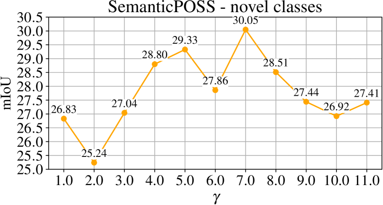
Figure 9: Ablation study analysing the difference in performance when changing the value of $\gamma$, the weighting factor of $\ell_{\text{A}}$. Reported performance are in terms of average mIoU of novel classes in the four splits of SemanticPOSS.

7 Conclusions

We explored the new problem of novel class discovery for 3D point cloud segmentation. Firstly, we adapted the only NCD method for 2D image semantic segmentation to 3D point cloud data, and experimentally found that it has several limitations. We discussed that extending 2D NCD approaches to 3D data (point clouds) is not trivial because the assumptions made for 2D data are not easily transferable to 3D. Secondly, we presented SNOPS, an extension of our original NOPS method, that tackles NCD for point cloud segmentation by using online clustering, uncertainty quantification and semantic distillation through a foundation model. We showed that the zero-shot accuracy of such foundation model alone is not satisfactory and we proved that by using it in combination with our SNOPS we can achieve higher performance. Lastly, we introduced a novel evaluation protocol to asses the performance of NCD in point cloud segmentation. Experiments on three different segmentation dataset showed that SNOPS outperforms the compared baselines by a large margin.

Limitations The first limitation of SNOPS is the prior knowledge on the number of novel classes $C_{n}$ to discover. This could be a limitation when $C_{n}$ is not a known prior and novel classes appear in an incremental manner. We believe that a solution may be to learn novel classes incrementally, as for example proposed by [50] in the 2D Novel Class Discovery literature. Finally, SNOPS lacks a mechanism to prevent drift when the auxiliary network outputs inaccurate features for novel classes. SNOPS may benefit the introduction of a filtering mechanism to avoid point features when the auxiliary network exhibits high uncertainty, as for example proposed by [53].

References

- \bibcommenthead
- Achlioptas \BOthers. [\APACyear2018] \APACinsertmetastarachlioptas2018learning{APACrefauthors}Achlioptas, P., Diamanti, O., Mitliagkas, I.\BCBL Guibas, L. \APACrefYearMonthDay2018. \BBOQ\APACrefatitleLearning representations and generative models for 3d point clouds Learning representations and generative models for 3d point clouds.\BBCQ \APACrefbtitleICCV. Iccv. \PrintBackRefs\CurrentBib
- Alonso \BOthers. [\APACyear2020] \APACinsertmetastaralonso2020MiniNet3D{APACrefauthors}Alonso, I., Riazuelo, L., Montesano, L.\BCBL Murillo, A. \APACrefYearMonthDay2020. \BBOQ\APACrefatitle3D-MiniNet: Learning a 2D Representation from Point Clouds for Fast and Efficient 3D LiDAR Semantic Segmentation 3D-MiniNet: Learning a 2D representation from point clouds for fast and efficient 3D LiDAR semantic segmentation.\BBCQ \APACrefbtitleIROS. Iros. \PrintBackRefs\CurrentBib
- Armeni \BOthers. [\APACyear2016] \APACinsertmetastararmeni20163d{APACrefauthors}Armeni, I., Sener, O., Zamir, A.R., Jiang, H., Brilakis, I., Fischer, M.\BCBL Savarese, S. \APACrefYearMonthDay2016. \BBOQ\APACrefatitle3d semantic parsing of large-scale indoor spaces 3d semantic parsing of large-scale indoor spaces.\BBCQ \APACrefbtitleCVPR. Cvpr. \PrintBackRefs\CurrentBib
- Asano \BOthers. [\APACyear2020] \APACinsertmetastarAsano2020{APACrefauthors}Asano, Y., Rupprecht, C.\BCBL Vedaldi, A. \APACrefYearMonthDay2020. \BBOQ\APACrefatitleSelf-labelling via simultaneous clustering and representation learning Self-labelling via simultaneous clustering and representation learning.\BBCQ \APACrefbtitleICLR. Iclr. \PrintBackRefs\CurrentBib
- Behley \BOthers. [\APACyear2021] \APACinsertmetastarbehley2021ijrr{APACrefauthors}Behley, J., Garbade, M., Milioto, A., Quenzel, J., Behnke, S., Gall, J.\BCBL Stachniss, C. \APACrefYearMonthDay2021. \BBOQ\APACrefatitleTowards 3D LiDAR-based semantic scene understanding of 3D point cloud sequences: The SemanticKITTI Dataset Towards 3D LiDAR-based semantic scene understanding of 3D point cloud sequences: The SemanticKITTI Dataset.\BBCQ \APACrefbtitleIJRR. Ijrr. \PrintBackRefs\CurrentBib
- Behley \BOthers. [\APACyear2019] \APACinsertmetastarbehley2019semantickitti{APACrefauthors}Behley, J., Garbade, M., Milioto, A., Quenzel, J., Behnke, S., Stachniss, C.\BCBL Gall, J. \APACrefYearMonthDay2019. \BBOQ\APACrefatitleSemanticKITTI: A dataset for semantic scene understanding of LiDAR sequences SemanticKITTI: A dataset for semantic scene understanding of LiDAR sequences.\BBCQ \APACrefbtitleCVPR. Cvpr. \PrintBackRefs\CurrentBib
- Caron \BOthers. [\APACyear2020] \APACinsertmetastarcaron2020unsupervised{APACrefauthors}Caron, M., Misra, I., Mairal, J., Goyal, P., Bojanowski, P.\BCBL Joulin, A. \APACrefYearMonthDay2020. \BBOQ\APACrefatitleUnsupervised learning of visual features by contrasting cluster assignments Unsupervised learning of visual features by contrasting cluster assignments.\BBCQ \APACrefbtitleNeurIPS. Neurips. \PrintBackRefs\CurrentBib
- Cen \BOthers. [\APACyear2022] \APACinsertmetastarcen2022open{APACrefauthors}Cen, J., Yun, P., Zhang, S., Cai, J., Luan, D., Tang, M.\BDBLWang, M. \APACrefYearMonthDay2022. \BBOQ\APACrefatitleOpen-world semantic segmentation for lidar point clouds Open-world semantic segmentation for lidar point clouds.\BBCQ \APACrefbtitleECCV. Eccv. \PrintBackRefs\CurrentBib
- Chen \BOthers. [\APACyear2017] \APACinsertmetastarchen2017deeplab{APACrefauthors}Chen, L., Papandreou, G., Kokkinos, I., Murphy, K.\BCBL Yuille, A. \APACrefYearMonthDay2017. \BBOQ\APACrefatitleDeeplab: Semantic image segmentation with deep convolutional nets, atrous convolution, and fully connected crfs Deeplab: Semantic image segmentation with deep convolutional nets, atrous convolution, and fully connected crfs.\BBCQ \APACrefbtitleT-PAMI. T-pami. \PrintBackRefs\CurrentBib
- Chen \BOthers. [\APACyear2018] \APACinsertmetastardeeplabv3plus2018{APACrefauthors}Chen, L., Zhu, Y., Papandreou, G., Schroff, F.\BCBL Hartwig, A. \APACrefYearMonthDay2018. \BBOQ\APACrefatitleEncoder-Decoder with Atrous Separable Convolution for Semantic Image Segmentation Encoder-decoder with atrous separable convolution for semantic image segmentation.\BBCQ \APACrefbtitleECCV. Eccv. \PrintBackRefs\CurrentBib
- Cheng \BOthers. [\APACyear2021] \APACinsertmetastarran2021af2s3net{APACrefauthors}Cheng, R., Razani, R., Taghavi, E., Li, E.\BCBL Liu, B. \APACrefYearMonthDay2021. \BBOQ\APACrefatitle(AF)2-S3Net: Attentive Feature Fusion with Adaptive Feature Selection for Sparse Semantic Segmentation Network (AF)2-S3Net: Attentive Feature Fusion with Adaptive Feature Selection for Sparse Semantic Segmentation Network.\BBCQ \APACrefbtitleCVPR. Cvpr. \PrintBackRefs\CurrentBib
- Choy \BOthers. [\APACyear2019] \APACinsertmetastarchoy20194d{APACrefauthors}Choy, C., Gwak, J.\BCBL Savarese, S. \APACrefYearMonthDay2019. \BBOQ\APACrefatitle4D spatio-temporal convnets: Minkowski convolutional neural networks 4D spatio-temporal convnets: Minkowski convolutional neural networks.\BBCQ \APACrefbtitleCVPR. Cvpr. \PrintBackRefs\CurrentBib
- Cuturi [\APACyear2013] \APACinsertmetastarcuturi2013sinkhorn{APACrefauthors}Cuturi, M. \APACrefYearMonthDay2013. \BBOQ\APACrefatitleSinkhorn distances: Lightspeed computation of optimal transport Sinkhorn distances: Lightspeed computation of optimal transport.\BBCQ \APACrefbtitleNeurIPS. Neurips. \PrintBackRefs\CurrentBib
- Deng \BOthers. [\APACyear2018] \APACinsertmetastardeng2018ppf{APACrefauthors}Deng, H., Birdal, T.\BCBL Ilic, S. \APACrefYearMonthDay2018. \BBOQ\APACrefatitlePpf-foldnet: Unsupervised learning of rotation invariant 3d local descriptors Ppf-foldnet: Unsupervised learning of rotation invariant 3d local descriptors.\BBCQ \APACrefbtitleECCV. Eccv. \PrintBackRefs\CurrentBib
- Dong \BOthers. [\APACyear2023] \APACinsertmetastardong2023maskclip{APACrefauthors}Dong, X., Bao, J., Zheng, Y.\BCBL \BOthersPeriod. \APACrefYearMonthDay2023. \BBOQ\APACrefatitleMaskclip: Masked self-distillation advances contrastive language-image pretraining Maskclip: Masked self-distillation advances contrastive language-image pretraining.\BBCQ \APACrefbtitleCVPR. Cvpr. \PrintBackRefs\CurrentBib
- Fini \BOthers. [\APACyear2021] \APACinsertmetastarfini2021unified{APACrefauthors}Fini, E., Sangineto, E., Lathuiliere, S., Zhong, Z., Nabi, M.\BCBL Ricci, E. \APACrefYearMonthDay2021. \BBOQ\APACrefatitleA unified objective for novel class discovery A unified objective for novel class discovery.\BBCQ \APACrefbtitleCVPR. Cvpr. \PrintBackRefs\CurrentBib
- Gadelha \BOthers. [\APACyear2020] \APACinsertmetastargadelha2020label{APACrefauthors}Gadelha, M., RoyChowdhury, A., Sharma, G., Kalogerakis, E., Cao, L., Learned-Miller, E.\BDBLMaji, S. \APACrefYearMonthDay2020. \BBOQ\APACrefatitleLabel-efficient learning on point clouds using approximate convex decompositions Label-efficient learning on point clouds using approximate convex decompositions.\BBCQ \APACrefbtitleECCV. Eccv. \PrintBackRefs\CurrentBib
- Geiger \BOthers. [\APACyear2012] \APACinsertmetastargeiger2012cvpr{APACrefauthors}Geiger, A., Lenz, P.\BCBL Urtasun, R. \APACrefYearMonthDay2012. \BBOQ\APACrefatitleAre we ready for Autonomous Driving? The KITTI Vision Benchmark Suite Are we ready for Autonomous Driving? The KITTI Vision Benchmark Suite.\BBCQ \APACrefbtitleCVPR. Cvpr. \PrintBackRefs\CurrentBib
- Giuliari \BOthers. [\APACyear2022] \APACinsertmetastarGiugliari2022{APACrefauthors}Giuliari, F., Skender, G., Cristani, M., Wang, Y.\BCBL Bue, A.D. \APACrefYearMonthDay2022. \BBOQ\APACrefatitleSpatial Commonsense Graph for Object Localisation in Partial Scenes Spatial commonsense graph for object localisation in partial scenes.\BBCQ \APACrefbtitleCVPR. Cvpr. \PrintBackRefs\CurrentBib
- Graham \BOthers. [\APACyear2018] \APACinsertmetastar3DSemanticSegmentationWithSubmanifoldSparseConvNet{APACrefauthors}Graham, B., Engelcke, M.\BCBL van der Maaten, L. \APACrefYearMonthDay2018. \BBOQ\APACrefatitle3D Semantic Segmentation with Submanifold Sparse Convolutional Networks 3D semantic segmentation with submanifold sparse convolutional networks.\BBCQ \APACrefbtitleCVPR. Cvpr. \PrintBackRefs\CurrentBib
- Graham \BBA van der Maaten [\APACyear2017] \APACinsertmetastarSubmanifoldSparseConvNet{APACrefauthors}Graham, B.\BCBT \BBA van der Maaten, L. \APACrefYearMonthDay2017. \BBOQ\APACrefatitleSubmanifold Sparse Convolutional Networks Submanifold sparse convolutional networks.\BBCQ \APACjournalVolNumPagesarXiv, \PrintBackRefs\CurrentBib
- Guzhov \BOthers. [\APACyear2022] \APACinsertmetastarguzhov2022audioclip{APACrefauthors}Guzhov, A., Raue, F., Hees, J.\BCBL Dengel, A. \APACrefYearMonthDay2022. \BBOQ\APACrefatitleAudioclip: Extending clip to image, text and audio Audioclip: Extending clip to image, text and audio.\BBCQ \APACrefbtitleICASSP. Icassp. \PrintBackRefs\CurrentBib
- Han \BOthers. [\APACyear2019] \APACinsertmetastarhan2019learning{APACrefauthors}Han, K., Vedaldi, A.\BCBL Zisserman, A. \APACrefYearMonthDay2019. \BBOQ\APACrefatitleLearning to discover novel visual categories via deep transfer clustering Learning to discover novel visual categories via deep transfer clustering.\BBCQ \APACrefbtitleCVPR. Cvpr. \PrintBackRefs\CurrentBib
- Hinton \BBA Salakhutdinov [\APACyear2006] \APACinsertmetastarhinton2006reducing{APACrefauthors}Hinton, G.\BCBT \BBA Salakhutdinov, R. \APACrefYearMonthDay2006. \BBOQ\APACrefatitleReducing the dimensionality of data with neural networks Reducing the dimensionality of data with neural networks.\BBCQ \APACjournalVolNumPagesScience, \PrintBackRefs\CurrentBib
- Hu \BOthers. [\APACyear2020] \APACinsertmetastarhu2020randla{APACrefauthors}Hu, Q., Yang, B., Xie, L., Rosa, S., Guo, Y., Wang, Z.\BDBLMarkham, A. \APACrefYearMonthDay2020. \BBOQ\APACrefatitleRandla-net: Efficient semantic segmentation of large-scale point clouds Randla-net: Efficient semantic segmentation of large-scale point clouds.\BBCQ \APACrefbtitleCVPR. Cvpr. \PrintBackRefs\CurrentBib
- Huang \BOthers. [\APACyear2021] \APACinsertmetastarhuang2021spatio{APACrefauthors}Huang, S., Xie, Y., Zhu, S.\BCBL Zhu, Y. \APACrefYearMonthDay2021. \BBOQ\APACrefatitleSpatio-temporal self-supervised representation learning for 3d point clouds Spatio-temporal self-supervised representation learning for 3d point clouds.\BBCQ \APACrefbtitleICCV. Iccv. \PrintBackRefs\CurrentBib
- Jatavallabhula \BBA et al. [\APACyear2023] \APACinsertmetastarjatavallabhula2023conceptfusion{APACrefauthors}Jatavallabhula, K.M.\BCBT \BBA et al., A.K. \APACrefYearMonthDay2023. \BBOQ\APACrefatitleConceptfusion: Open-set multimodal 3d mapping Conceptfusion: Open-set multimodal 3d mapping.\BBCQ \APACjournalVolNumPagesarXiv, \PrintBackRefs\CurrentBib
- Ji \BOthers. [\APACyear2019] \APACinsertmetastarji2019invariant{APACrefauthors}Ji, X., Henriques, J.\BCBL Vedaldi, A. \APACrefYearMonthDay2019. \BBOQ\APACrefatitleInvariant information clustering for unsupervised image classification and segmentation Invariant information clustering for unsupervised image classification and segmentation.\BBCQ \APACrefbtitleICCV. Iccv. \PrintBackRefs\CurrentBib
- Jia \BOthers. [\APACyear2021] \APACinsertmetastarjia2021joint{APACrefauthors}Jia, X., Han, K., Zhu, Y.\BCBL Green, B. \APACrefYearMonthDay2021. \BBOQ\APACrefatitleJoint representation learning and novel category discovery on single-and multi-modal data Joint representation learning and novel category discovery on single-and multi-modal data.\BBCQ \APACrefbtitleICCV. Iccv. \PrintBackRefs\CurrentBib
- Jiang \BOthers. [\APACyear2021] \APACinsertmetastarjiang2021sampling{APACrefauthors}Jiang, H., Shen, Y., Xie, J., Li, J., Qian, J.\BCBL Yang, J. \APACrefYearMonthDay2021. \BBOQ\APACrefatitleSampling network guided cross-entropy method for unsupervised point cloud registration Sampling network guided cross-entropy method for unsupervised point cloud registration.\BBCQ \APACrefbtitleICCV. Iccv. \PrintBackRefs\CurrentBib
- Joseph \BOthers. [\APACyear2022] \APACinsertmetastarjoseph2022novel{APACrefauthors}Joseph, K., Paul, S., Aggarwal, G., Biswas, S., Rai, P., Han, K.\BCBL Balasubramanian, V. \APACrefYearMonthDay2022. \BBOQ\APACrefatitleNovel Class Discovery without Forgetting Novel class discovery without forgetting.\BBCQ \APACjournalVolNumPagesECCV, \PrintBackRefs\CurrentBib
- Kirillov \BOthers. [\APACyear2023] \APACinsertmetastarkirillov2023segment{APACrefauthors}Kirillov, A., Mintun, E., Ravi, N., Mao, H., Rolland, C., Gustafson, L.\BDBLothers \APACrefYearMonthDay2023. \BBOQ\APACrefatitleSegment anything Segment anything.\BBCQ \APACjournalVolNumPagesarXiv preprint arXiv:2304.02643, \PrintBackRefs\CurrentBib
- Li \BOthers. [\APACyear2019] \APACinsertmetastarli2019pu{APACrefauthors}Li, R., Li, X., Fu, C., Cohen-Or, D.\BCBL Heng, P. \APACrefYearMonthDay2019. \BBOQ\APACrefatitlePu-gan: a point cloud upsampling adversarial network Pu-gan: a point cloud upsampling adversarial network.\BBCQ \APACrefbtitleICCV. Iccv. \PrintBackRefs\CurrentBib
- Mei \BOthers. [\APACyear2023] \APACinsertmetastarmei2023overlap{APACrefauthors}Mei, G., Poiesi, F., Saltori, C., Zhang, J., Ricci, E.\BCBL Sebe, N. \APACrefYearMonthDay2023. \BBOQ\APACrefatitleOverlap-guided Gaussian Mixture Models for Point Cloud Registration Overlap-guided gaussian mixture models for point cloud registration.\BBCQ \APACrefbtitleWACV. Wacv. \PrintBackRefs\CurrentBib
- Mei \BOthers. [\APACyear2022] \APACinsertmetastarmei2022data{APACrefauthors}Mei, G., Saltori, C., Poiesi, F., Zhang, J., Ricci, E., Sebe, N.\BCBL Wu, Q. \APACrefYearMonthDay2022. \BBOQ\APACrefatitleData Augmentation-free Unsupervised Learning for 3D Point Cloud Understanding Data augmentation-free unsupervised learning for 3d point cloud understanding.\BBCQ \APACrefbtitleBMVC. Bmvc. \PrintBackRefs\CurrentBib
- Milioto \BOthers. [\APACyear2019] \APACinsertmetastarmilioto2019rangenet++{APACrefauthors}Milioto, A., Vizzo, I., Behley, J.\BCBL Stachniss, C. \APACrefYearMonthDay2019. \BBOQ\APACrefatitleRangenet++: Fast and accurate lidar semantic segmentation Rangenet++: Fast and accurate lidar semantic segmentation.\BBCQ \APACrefbtitleIROS. Iros. \PrintBackRefs\CurrentBib
- Miller [\APACyear1995] \APACinsertmetastarmiller1995wordnet{APACrefauthors}Miller, G.A. \APACrefYearMonthDay1995. \BBOQ\APACrefatitleWordNet: a lexical database for English Wordnet: a lexical database for english.\BBCQ \APACjournalVolNumPagesCommunications of the ACM, \PrintBackRefs\CurrentBib
- Pan \BOthers. [\APACyear2020] \APACinsertmetastarpan2020semanticposs{APACrefauthors}Pan, Y., Gao, B., Mei, J., Geng, S., Li, C.\BCBL Zhao, H. \APACrefYearMonthDay2020. \BBOQ\APACrefatitleSemanticPOSS: A point cloud dataset with large quantity of dynamic instances SemanticPOSS: A point cloud dataset with large quantity of dynamic instances.\BBCQ \APACrefbtitleIV. Iv. \PrintBackRefs\CurrentBib
- Pang \BOthers. [\APACyear2022] \APACinsertmetastarpang2022masked{APACrefauthors}Pang, Y., Wang, X., Tay, F.E., Liu, W., Tian, Y.\BCBL Yuan, L. \APACrefYearMonthDay2022. \BBOQ\APACrefatitleMasked autoencoders for point cloud self-supervised learning Masked autoencoders for point cloud self-supervised learning.\BBCQ \APACrefbtitleECCV. Eccv. \PrintBackRefs\CurrentBib
- Peng \BBA et al. [\APACyear2023] \APACinsertmetastarpeng2023openscene{APACrefauthors}Peng, S.\BCBT \BBA et al., K.G. \APACrefYearMonthDay2023. \BBOQ\APACrefatitleOpenscene: 3d scene understanding with open vocabularies Openscene: 3d scene understanding with open vocabularies.\BBCQ \APACrefbtitleCVPR. Cvpr. \PrintBackRefs\CurrentBib
- Poiesi \BBA Boscaini [\APACyear2023] \APACinsertmetastarpoiesi2022learning{APACrefauthors}Poiesi, F.\BCBT \BBA Boscaini, D. \APACrefYearMonthDay2023. \BBOQ\APACrefatitleLearning general and distinctive 3D local deep descriptors for point cloud registration Learning general and distinctive 3d local deep descriptors for point cloud registration.\BBCQ \APACjournalVolNumPagesT-PAMI, \PrintBackRefs\CurrentBib
- Poursaeed \BOthers. [\APACyear2020] \APACinsertmetastarpoursaeed2020self{APACrefauthors}Poursaeed, O., Jiang, T., Qiao, H., Xu, N.\BCBL Kim, V.G. \APACrefYearMonthDay2020. \BBOQ\APACrefatitleSelf-supervised learning of point clouds via orientation estimation Self-supervised learning of point clouds via orientation estimation.\BBCQ \APACrefbtitle3DV. 3dv. \PrintBackRefs\CurrentBib
- Qi, Su\BCBL \BOthers. [\APACyear2017] \APACinsertmetastarqi2017pointnet{APACrefauthors}Qi, C., Su, H., Mo, K.\BCBL Guibas, L. \APACrefYearMonthDay2017. \BBOQ\APACrefatitlePointnet: Deep learning on point sets for 3D classification and segmentation Pointnet: Deep learning on point sets for 3D classification and segmentation.\BBCQ \APACrefbtitleCVPR. Cvpr. \PrintBackRefs\CurrentBib
- Qi, Yi\BCBL \BOthers. [\APACyear2017] \APACinsertmetastarqi2017pointnet++{APACrefauthors}Qi, C., Yi, L., Su, H.\BCBL Guibas, L. \APACrefYearMonthDay2017. \BBOQ\APACrefatitlePointnet++: Deep hierarchical feature learning on point sets in a metric space Pointnet++: Deep hierarchical feature learning on point sets in a metric space.\BBCQ \APACrefbtitleNeurIPS. Neurips. \PrintBackRefs\CurrentBib
- Qian \BOthers. [\APACyear2021] \APACinsertmetastarqian2021pu{APACrefauthors}Qian, G., Abualshour, A., Li, G., Thabet, A.\BCBL Ghanem, B. \APACrefYearMonthDay2021. \BBOQ\APACrefatitlePu-gcn: Point cloud upsampling using graph convolutional networks Pu-gcn: Point cloud upsampling using graph convolutional networks.\BBCQ \APACrefbtitleCVPR. Cvpr. \PrintBackRefs\CurrentBib
- Radford, Kim\BCBL \BBA et al. [\APACyear2021] \APACinsertmetastarradford2021learning{APACrefauthors}Radford, A., Kim, J.\BCBL et al., C.H. \APACrefYearMonthDay2021. \BBOQ\APACrefatitleLearning transferable visual models from natural language supervision Learning transferable visual models from natural language supervision.\BBCQ \APACrefbtitleICML. Icml. \PrintBackRefs\CurrentBib
- Radford, Kim, Hallacy\BCBL \BOthers. [\APACyear2021] \APACinsertmetastarradford2021clip{APACrefauthors}Radford, A., Kim, J.W., Hallacy, C., Ramesh, A., Goh, G., Agarwal, S.\BDBLSutskever, I. \APACrefYearMonthDay2021. \BBOQ\APACrefatitleLearning transferable visual models from natural language supervision Learning transferable visual models from natural language supervision.\BBCQ \APACrefbtitleICML. Icml. \PrintBackRefs\CurrentBib
- Riz \BOthers. [\APACyear2023] \APACinsertmetastarriz2023novel{APACrefauthors}Riz, L., Saltori, C., Ricci, E.\BCBL Poiesi, F. \APACrefYearMonthDay2023. \BBOQ\APACrefatitleNovel Class Discovery for 3D Point Cloud Semantic Segmentation Novel class discovery for 3d point cloud semantic segmentation.\BBCQ \APACrefbtitleCVPR. Cvpr. \PrintBackRefs\CurrentBib
- Ronneberger \BOthers. [\APACyear2015] \APACinsertmetastarronneberger2015u{APACrefauthors}Ronneberger, O., Fischer, P.\BCBL Brox, T. \APACrefYearMonthDay2015. \BBOQ\APACrefatitleU-net: Convolutional networks for biomedical image segmentation U-net: Convolutional networks for biomedical image segmentation.\BBCQ \APACrefbtitleMICCAI. Miccai. \PrintBackRefs\CurrentBib
- Roy \BOthers. [\APACyear2022] \APACinsertmetastarroy2022class{APACrefauthors}Roy, S., Liu, M., Zhong, Z., Sebe, N.\BCBL Ricci, E. \APACrefYearMonthDay2022. \BBOQ\APACrefatitleClass-incremental Novel Class Discovery Class-incremental novel class discovery.\BBCQ \APACrefbtitleECCV. Eccv. \PrintBackRefs\CurrentBib
- Rozenberszki \BOthers. [\APACyear2022] \APACinsertmetastarrozenberszki2022language{APACrefauthors}Rozenberszki, D., Litany, O.\BCBL Dai, A. \APACrefYearMonthDay2022. \BBOQ\APACrefatitleLanguage-grounded indoor 3D semantic segmentation in the wild Language-grounded indoor 3d semantic segmentation in the wild.\BBCQ \APACrefbtitleECCV. Eccv. \PrintBackRefs\CurrentBib
- Saltori, Galasso\BCBL \BOthers. [\APACyear2022] \APACinsertmetastarsaltori2022cosmix{APACrefauthors}Saltori, C., Galasso, F., Fiameni, G., Sebe, N., Ricci, E.\BCBL Poiesi, F. \APACrefYearMonthDay2022. \BBOQ\APACrefatitleCosmix: Compositional semantic mix for domain adaptation in 3d lidar segmentation Cosmix: Compositional semantic mix for domain adaptation in 3d lidar segmentation.\BBCQ \APACrefbtitleECCV. Eccv. \PrintBackRefs\CurrentBib
- Saltori, Krivosheev\BCBL \BOthers. [\APACyear2022] \APACinsertmetastarsaltori2022gipso{APACrefauthors}Saltori, C., Krivosheev, E., Lathuiliére, S., Sebe, N., Galasso, F., Fiameni, G.\BDBLPoiesi, F. \APACrefYearMonthDay2022. \BBOQ\APACrefatitleGipso: Geometrically informed propagation for online adaptation in 3d lidar segmentation Gipso: Geometrically informed propagation for online adaptation in 3d lidar segmentation.\BBCQ \APACrefbtitleECCV. Eccv. \PrintBackRefs\CurrentBib
- Sauder \BBA Sievers [\APACyear2019] \APACinsertmetastarsauder2019self{APACrefauthors}Sauder, J.\BCBT \BBA Sievers, B. \APACrefYearMonthDay2019. \BBOQ\APACrefatitleSelf-supervised deep learning on point clouds by reconstructing space Self-supervised deep learning on point clouds by reconstructing space.\BBCQ \APACjournalVolNumPagesNeurIPS, \PrintBackRefs\CurrentBib
- Shu \BOthers. [\APACyear2019] \APACinsertmetastarshu20193d{APACrefauthors}Shu, D.W., Park, S.W.\BCBL Kwon, J. \APACrefYearMonthDay2019. \BBOQ\APACrefatitle3d point cloud generative adversarial network based on tree structured graph convolutions 3d point cloud generative adversarial network based on tree structured graph convolutions.\BBCQ \APACrefbtitleICCV. Iccv. \PrintBackRefs\CurrentBib
- Song \BOthers. [\APACyear2021] \APACinsertmetastarRan2021{APACrefauthors}Song, R., Zhang, W., Zhao, Y., Liu, Y.\BCBL Rosin, P. \APACrefYearMonthDay2021. \BBOQ\APACrefatitleMesh Saliency: An Independent Perceptual Measure or A Derivative of Image Saliency? Mesh saliency: An independent perceptual measure or a derivative of image saliency?\BBCQ \APACrefbtitleCVPR. Cvpr. \PrintBackRefs\CurrentBib
- Souly \BOthers. [\APACyear2017] \APACinsertmetastarsouly2017semi{APACrefauthors}Souly, N., Spampinato, C.\BCBL Shah, M. \APACrefYearMonthDay2017. \BBOQ\APACrefatitleSemi supervised semantic segmentation using generative adversarial network Semi supervised semantic segmentation using generative adversarial network.\BBCQ \APACrefbtitleICCV. Iccv. \PrintBackRefs\CurrentBib
- Tang \BOthers. [\APACyear2016] \APACinsertmetastartang2016large{APACrefauthors}Tang, X., Wang, J., Gao, B., Dellandréa, E., Gaizauskas, R.\BCBL Chen, L. \APACrefYearMonthDay2016. \BBOQ\APACrefatitleLarge scale semi-supervised object detection using visual and semantic knowledge transfer Large scale semi-supervised object detection using visual and semantic knowledge transfer.\BBCQ \APACrefbtitleCVPR. Cvpr. \PrintBackRefs\CurrentBib
- Thomas \BOthers. [\APACyear2019] \APACinsertmetastarthomas2019kpconv{APACrefauthors}Thomas, H., Qi, C., Deschaud, J\BHBIE., Marcotegui, B., Goulette, F.\BCBL Guibas, J.L. \APACrefYearMonthDay2019. \BBOQ\APACrefatitleKpconv: Flexible and deformable convolution for point clouds Kpconv: Flexible and deformable convolution for point clouds.\BBCQ \APACrefbtitleICCV. Iccv. \PrintBackRefs\CurrentBib
- Van der Maaten \BBA Hinton [\APACyear2008] \APACinsertmetastarvan2008visualizing{APACrefauthors}Van der Maaten, L.\BCBT \BBA Hinton, G. \APACrefYearMonthDay2008. \BBOQ\APACrefatitleVisualizing data using t-SNE. Visualizing data using t-sne.\BBCQ \APACjournalVolNumPagesJournal of machine learning research, \PrintBackRefs\CurrentBib
- Vaze \BOthers. [\APACyear2022] \APACinsertmetastarvaze2022generalized{APACrefauthors}Vaze, S., Han, K., Vedaldi, A.\BCBL Zisserman, A. \APACrefYearMonthDay2022. \BBOQ\APACrefatitleGeneralized category discovery Generalized category discovery.\BBCQ \APACrefbtitleCVPR. Cvpr. \PrintBackRefs\CurrentBib
- Wen \BOthers. [\APACyear2020] \APACinsertmetastarwen2020point{APACrefauthors}Wen, X., Li, T., Han, Z.\BCBL Liu, Y. \APACrefYearMonthDay2020. \BBOQ\APACrefatitlePoint cloud completion by skip-attention network with hierarchical folding Point cloud completion by skip-attention network with hierarchical folding.\BBCQ \APACrefbtitleCVPR. Cvpr. \PrintBackRefs\CurrentBib
- B. Wu \BOthers. [\APACyear2018] \APACinsertmetastarwu2018squeezeseg{APACrefauthors}Wu, B., Wan, A., Yue, X.\BCBL Keutzer, K. \APACrefYearMonthDay2018. \BBOQ\APACrefatitleSqueezeseg: Convolutional neural nets with recurrent CRF for real-time road-object segmentation from 3D LiDAR point cloud Squeezeseg: Convolutional neural nets with recurrent CRF for real-time road-object segmentation from 3D LiDAR point cloud.\BBCQ \APACrefbtitleICRA. Icra. \PrintBackRefs\CurrentBib
- B. Wu \BOthers. [\APACyear2019] \APACinsertmetastarwu2019squeezesegv2{APACrefauthors}Wu, B., Zhou, X., Zhao, S., Yue, X.\BCBL Keutzer, K. \APACrefYearMonthDay2019. \BBOQ\APACrefatitleSqueezesegv2: Improved model structure and unsupervised domain adaptation for road-object segmentation from a LiDAR point cloud Squeezesegv2: Improved model structure and unsupervised domain adaptation for road-object segmentation from a LiDAR point cloud.\BBCQ \APACrefbtitleICRA. Icra. \PrintBackRefs\CurrentBib
- J. Wu \BOthers. [\APACyear2016] \APACinsertmetastarwu2016learning{APACrefauthors}Wu, J., Zhang, C., Xue, T., Freeman, B.\BCBL Tenenbaum, J. \APACrefYearMonthDay2016. \BBOQ\APACrefatitleLearning a probabilistic latent space of object shapes via 3d generative-adversarial modeling Learning a probabilistic latent space of object shapes via 3d generative-adversarial modeling.\BBCQ \PrintBackRefs\CurrentBib
- Xiao \BOthers. [\APACyear2023] \APACinsertmetastarxiao2023tpami{APACrefauthors}Xiao, A., Huang, J., Guan, D., Zhang, X., Lu, S.\BCBL Shao, L. \APACrefYearMonthDay2023. \BBOQ\APACrefatitleUnsupervised point cloud representation learning with deep neural networks: A survey Unsupervised point cloud representation learning with deep neural networks: A survey.\BBCQ \APACjournalVolNumPagesT-PAMI, \PrintBackRefs\CurrentBib
- Xie \BOthers. [\APACyear2020] \APACinsertmetastarxie2020pointcontrast{APACrefauthors}Xie, S., Gu, J., Guo, D., Qi, C.R., Guibas, L.\BCBL Litany, O. \APACrefYearMonthDay2020. \BBOQ\APACrefatitlePointcontrast: Unsupervised pre-training for 3d point cloud understanding Pointcontrast: Unsupervised pre-training for 3d point cloud understanding.\BBCQ \APACrefbtitleECCV. Eccv. \PrintBackRefs\CurrentBib
- G. Yang \BOthers. [\APACyear2019] \APACinsertmetastaryang2019pointflow{APACrefauthors}Yang, G., Huang, X., Hao, Z., Liu, M., Belongie, S.\BCBL Hariharan, B. \APACrefYearMonthDay2019. \BBOQ\APACrefatitlePointflow: 3d point cloud generation with continuous normalizing flows Pointflow: 3d point cloud generation with continuous normalizing flows.\BBCQ \APACrefbtitleICCV. Iccv. \PrintBackRefs\CurrentBib
- M. Yang \BOthers. [\APACyear2022] \APACinsertmetastaryang2022divide{APACrefauthors}Yang, M., Zhu, Y., Yu, J., Wu, A.\BCBL Deng, C. \APACrefYearMonthDay2022. \BBOQ\APACrefatitleDivide and Conquer: Compositional Experts for Generalized Novel Class Discovery Divide and conquer: Compositional experts for generalized novel class discovery.\BBCQ \APACrefbtitleCVPR. Cvpr. \PrintBackRefs\CurrentBib
- Y. Yang \BOthers. [\APACyear2021] \APACinsertmetastaryang2021progressive{APACrefauthors}Yang, Y., Ahn, P., Kim, D., Lee, H.\BCBL Kim, J. \APACrefYearMonthDay2021. \BBOQ\APACrefatitleProgressive seed generation auto-encoder for unsupervised point cloud learning Progressive seed generation auto-encoder for unsupervised point cloud learning.\BBCQ \APACrefbtitleICCV. Iccv. \PrintBackRefs\CurrentBib
- Y. Yang \BOthers. [\APACyear2018] \APACinsertmetastaryang2018foldingnet{APACrefauthors}Yang, Y., Feng, C., Shen, Y.\BCBL Tian, D. \APACrefYearMonthDay2018. \BBOQ\APACrefatitleFoldingnet: Point cloud auto-encoder via deep grid deformation Foldingnet: Point cloud auto-encoder via deep grid deformation.\BBCQ \APACrefbtitleCVPR. Cvpr. \PrintBackRefs\CurrentBib
- Yu \BOthers. [\APACyear2022] \APACinsertmetastaryu2022point{APACrefauthors}Yu, X., Tang, L., Rao, Y., Huang, T., Zhou, J.\BCBL Lu, J. \APACrefYearMonthDay2022. \BBOQ\APACrefatitlePoint-bert: Pre-training 3d point cloud transformers with masked point modeling Point-bert: Pre-training 3d point cloud transformers with masked point modeling.\BBCQ \APACrefbtitleCVPR. Cvpr. \PrintBackRefs\CurrentBib
- Yuan \BOthers. [\APACyear2018] \APACinsertmetastaryuan2018pcn{APACrefauthors}Yuan, W., Khot, T., Held, D., Mertz, C.\BCBL Hebert, M. \APACrefYearMonthDay2018. \BBOQ\APACrefatitlePcn: Point completion network Pcn: Point completion network.\BBCQ \APACrefbtitle3DV. 3dv. \PrintBackRefs\CurrentBib
- L. Zhang \BBA Qi [\APACyear2020] \APACinsertmetastarzhang2020wcp{APACrefauthors}Zhang, L.\BCBT \BBA Qi, G. \APACrefYearMonthDay2020. \BBOQ\APACrefatitleWcp: Worst-case perturbations for semi-supervised deep learning Wcp: Worst-case perturbations for semi-supervised deep learning.\BBCQ \APACrefbtitleCVPR. Cvpr. \PrintBackRefs\CurrentBib
- Y. Zhang \BOthers. [\APACyear2020] \APACinsertmetastarzhang2020polarnet{APACrefauthors}Zhang, Y., Zhou, Z., David, P., Yue, X., Xi, Z., Gong, B.\BCBL Foroosh, H. \APACrefYearMonthDay2020. \BBOQ\APACrefatitlePolarnet: An improved grid representation for online LiDAR point clouds semantic segmentation Polarnet: An improved grid representation for online LiDAR point clouds semantic segmentation.\BBCQ \APACrefbtitleCVPR. Cvpr. \PrintBackRefs\CurrentBib
- Z. Zhang \BOthers. [\APACyear2021] \APACinsertmetastarzhang2021self{APACrefauthors}Zhang, Z., Girdhar, R., Joulin, A.\BCBL I. Misra, I. \APACrefYearMonthDay2021. \BBOQ\APACrefatitleSelf-supervised pretraining of 3d features on any point-cloud Self-supervised pretraining of 3d features on any point-cloud.\BBCQ \APACrefbtitleICCV. Iccv. \PrintBackRefs\CurrentBib
- Zhao \BOthers. [\APACyear2022] \APACinsertmetastarzhao2022novel{APACrefauthors}Zhao, Y., Zhong, Z., Sebe, N.\BCBL Lee, G. \APACrefYearMonthDay2022. \BBOQ\APACrefatitleNovel Class Discovery in Semantic Segmentation Novel class discovery in semantic segmentation.\BBCQ \APACrefbtitleCVPR. Cvpr. \PrintBackRefs\CurrentBib
- Zhong, Fini\BCBL \BOthers. [\APACyear2021] \APACinsertmetastarzhong2021neighborhood{APACrefauthors}Zhong, Z., Fini, E., Roy, S., Luo, Z., Ricci, E.\BCBL Sebe, N. \APACrefYearMonthDay2021. \BBOQ\APACrefatitleNeighborhood contrastive learning for novel class discovery Neighborhood contrastive learning for novel class discovery.\BBCQ \APACrefbtitleCVPR. Cvpr. \PrintBackRefs\CurrentBib
- Zhong, Zhu\BCBL \BOthers. [\APACyear2021] \APACinsertmetastarzhong2021openmix{APACrefauthors}Zhong, Z., Zhu, L., Luo, Z., Li, S., Yang, Y.\BCBL Sebe, N. \APACrefYearMonthDay2021. \BBOQ\APACrefatitleOpenmix: Reviving known knowledge for discovering novel visual categories in an open world Openmix: Reviving known knowledge for discovering novel visual categories in an open world.\BBCQ \APACrefbtitleCVPR. Cvpr. \PrintBackRefs\CurrentBib
- Zhou \BBA Tuzel [\APACyear2018] \APACinsertmetastarzhou2018voxelnet{APACrefauthors}Zhou, Y.\BCBT \BBA Tuzel, O. \APACrefYearMonthDay2018. \BBOQ\APACrefatitleVoxelnet: End-to-end learning for point cloud based 3D object detection Voxelnet: End-to-end learning for point cloud based 3D object detection.\BBCQ \APACrefbtitleCVPR. Cvpr. \PrintBackRefs\CurrentBib
- Zhu \BOthers. [\APACyear2021] \APACinsertmetastarzhu2021cylindrical{APACrefauthors}Zhu, X., Zhou, H., Wang, T., Hong, F., Ma, Y., Li, W.\BDBLLin, D. \APACrefYearMonthDay2021. \BBOQ\APACrefatitleCylindrical and asymmetrical 3D convolution networks for lidar segmentation Cylindrical and asymmetrical 3D convolution networks for lidar segmentation.\BBCQ \APACrefbtitleCVPR. Cvpr. \PrintBackRefs\CurrentBib