Lite-Mind: Towards Efficient and Versatile Brain Representation Network

Abstract

Research in decoding visual information from the brain, particularly through the non-invasive fMRI method, is rapidly progressing. The challenge arises from the limited data availability and the low signal-to-noise ratio of fMRI signals, leading to a low-precision task of fMRI-to-image retrieval. State-of-the-art MindEye remarkably improves fMRI-to-image retrieval performance by leveraging a deep MLP with a high parameter count orders of magnitude, i.e., a 996M MLP Backbone per subject, to align fMRI embeddings to the final hidden layer of CLIP’s vision transformer. However, significant individual variations exist among subjects, even within identical experimental setups, mandating the training of subject-specific models. The substantial parameters pose significant challenges in deploying fMRI decoding on practical devices, especially with the necessitating of specific models for each subject. To this end, we propose Lite-Mind, a lightweight, efficient, and versatile brain representation network based on discrete Fourier transform, that efficiently aligns fMRI voxels to fine-grained information of CLIP. Our experiments demonstrate that Lite-Mind achieves an impressive 94.3% fMRI-to-image retrieval accuracy on the NSD dataset for Subject 1, with 98.7% fewer parameters than MindEye. Lite-Mind is also proven to be able to be migrated to smaller brain datasets and establishes a new state-of-the-art for zero-shot classification on the GOD dataset. Code is available at https://github.com/gongzix/Lite-Mind.

1 Introduction

Brain decoding holds immense significance in elucidating intricate mental processes and serves as a pivotal technology for brain-computer interfaces [24, 14, 26]. Among diverse brain decoding tasks, the decoding of visual information stands out as a paramount yet challenging endeavor, allowing us to unravel the complex mechanisms involved in visual processing, object recognition, scene understanding, and even higher-order cognitive functions. In the pursuit of decoding natural visual information, functional magnetic resonance imaging (fMRI) is widely employed as a non-invasive modality to decipher the perceptual and semantic information intricately encoded within the cerebral cortex [20]. It draws considerable attention to fMRI-to-image retrieval/reconstruction tasks. This paper focuses primarily on tasks related to fMRI-to-image retrieval.

Figure 1: The significance of lightweight brain decoding model. Clouds of different colors represent different subject-wise models, and the size of the cloud represents the size of the model. The storage cost of MindEye is extremely high, and each person’s model parameter quantity is at the GB level, while Lite-Mind only requires the MB level parameter quantity.

The success of fMRI-to-image retrieval heavily relies on aligning fMRI signals with the representation space of images. However, fMRI data often suffers from spatial redundancy, noise, and sample sparsity, leading to poor representation of fMRI signals and potential overfitting to noise distribution for deep models. To address these challenges, previous studies have found ridge regression and shallow linear models to be effective solutions for fMRI-based models [27, 15, 9, 1, 13, 44]. Recently, it has been demonstrated the effectiveness of leveraging pretrained CLIP models [28] as a powerful bridge between fMRI voxels and images, since CLIP’s image embeddings capture fine-grained and semantic information of pictures [21, 23, 19, 33]. Initially, the CLS token of the CLIP image encoder was used to align voxels in Mind-Reader [19]. Considering the CLS token alone provides limited information for fMRI data, BrainClip [21] and UniBrain [23] introduce the text annotations of images to assist in aligning fMRI voxels with image representations. Brain-diffuser [25] aligns voxel representations with the last hidden layer of CLIP using large-scale linear models ($257\times 14$M) for the first time.

Among the CLIP-related models, MindEye [33] stands out by employing a large-scale (996M) MLP Backbone and Projector to map fMRI voxels and align their representations with the final hidden layer of CLIP using contrastive learning. MindEye achieves remarkable breakthroughs, surpassing $90\%$ accuracy for both image and brain retrieval, outperforming previous state-of-the-art accuracies that were below $50\%$. However, the practical application of large-scale models in brain science research faces limitations. Each subject’s fMRI data can exhibit significant variations, even within identical experimental setups, making it currently infeasible to establish a universal encoding model that performs well for all individuals. Consequently, training individual encoding models for each subject becomes necessary, as depicted in Figure 1. Apparently, it is impractical to expect hospitals to have access to computing resources with sufficient performance to train a unique large-scale model (e.g., MindEye) for each individual. Therefore, the ideal scenario involves equipping individuals with lightweight brain-computer interface edge devices, enabling image representations to be efficiently retrieved by a lightweight model. To this end, there is an urgent need to develop a brain network that is lightweight and efficient, as illustrated in the right segment of Figure 1, for practical implementation and deployment of brain-computer interfaces in real-world scenarios.

MindEye strongly benefits from an MLP backbone with a high parameter count, which allows for straightforward and powerful compression and preservation. However, when dealing with fMRI data, which typically has a low signal-to-noise ratio, an MLP focusing on voxel value-wise mappings may inadvertently suppress informative voxel signal values while being inefficient at reducing noisy values. This can lead to model parameter redundancy and decelerated convergence speed. Recently, the Fourier transform has gained attention in deep learning, demonstrating lightweight characteristics and improved efficiency in learning frequency domain patterns, due to its global perspective and energy concentration properties [38]. Additionally, the Fourier transform naturally possesses the advantage of processing signals: it is more effective and efficient to filter out noise and maintain informative voxel signals in the frequency domain. It presents a promising alternative to large-scale MLPs for encoding fMRI signals.

To tackle the trade-off between model capacity and scalability in fMRI-to-image retrieval, we propose Lite-Mind, a lightweight, efficient, and versatile brain representation network. We redesign MindEye with our elaborate Discrete Fourier Transform (DFT) Backbone, avoiding the heavy MLP Backbone used in MindEye. Extensive experiments show that Lite-Mind achieves 94.3% retrieval accuracy for Subject 1 on the NSD dataset, with 98.7% fewer parameters than MindEye. Lite-Mind also proves its adaptability to smaller brain datasets and establishes a new state-of-the-art zero-shot classification on the GOD dataset. Our contributions are summarized as follows:

• We empirically show that it is unnecessary to overly focus on each voxel value of fMRI-to-image retrieval while focusing on the global features of fMRI patches is more lightweight and efficient.

• We propose a new Brain Representation Network DFT Bcakbone based on Discrete Fourier Transform, as an efficient and versatile fMRI representation network for fMRI-to-image retrieval. Its effectiveness, efficiency, and lightweight are demonstrated.

• We migrated DFT Backbone to a smaller GOD dataset and demonstrated its universality. It achieves state-of-the-art zero-shot classification performance.

2 Related Work

2.1 Brain Visual Decoding

The study of visual decoding using fMRI in the human brain has been a long-standing endeavor. In the most important fMRI-image reconstruction and partial fMRI-image retrieval tasks, the foundation of performance is how to align fMRI signals to the image representation space or intermediate space. Due to the low signal-to-noise ratio of fMRI, the initial research emphasized using models based on linear regression to extract fMRI signals and images into the intermediate space for functional decoding of the human brain or reconstruction of faces and natural scenes. Further research utilizes pre-trained VGG to enrich hierarchical image features [13, 34, 7]. With the development of cross-modal tasks, the image-text pre-training model CLIP has been introduced into fMRI-image research. Mind-reader [19] is the first to adopt a contrastive learning approach, using the nsdgenal ROI region of NSD data and a shallow resnet-like model to align fMRI with the CLS token output by the CLIP image encoder. Mind-Reader did not achieve good performance in fMRI-image retrieval when using InfoNCE loss. BrainClip [21] uses a VAE model for retrieval tasks while still using the CLS token. Brain diffuser [25] introduced a fine-grained representation of the image of the last hidden layer in CLIP. But they used 257 different linear regression models to align each layer of the 257 hidden layers, resulting in the model being too cumbersome. Mind-Vis [5] conducted self-supervised mask pre-training on fMRI signals for another dataset, BOLD5000, and demonstrated that voxel patches can be used to process fMRI voxel values. Using a linear regression model, Takagi et al. [36] introduce additional ventral brain regions and align fMRI to the Stable Diffusion variable space. MindEye [33] uses a deep MLP backbone for contrastive learning, aligning the last hidden layer $257\times 768$ of CLIP, and using diffusion prior in DALLE·2 [29] for the first time to narrow the disjointed vectors. At the same time, it creatively proposed a mixed contrast loss MixCo as a data augmentation method to make the large model converge. However, to the best of our knowledge, no previous research has focused on lightweight and efficient brain networks.

2.2 Fourier Transform in Deep Learning

Fourier transform plays a vital role in the area of digital signal processing. It has been introduced to deep learning for enhanced learning performance [11, 8, 43]. GFNet [30] utilizes fast Fourier transform to convert images to the frequency domain and exchange global information between learnable filters. As a continuous global convolution independent of input resolution, Guibas et al. [12] design the adaptive Fourier neural operator frame token mixing. Xu et al. [41] devise a learning-based frequency selection method to identify trivial frequency components and improve the accuracy of classifying images. On text classification, Lee-Thorp et al. [18] use the Fourier transform as a text token mixing mechanism. Furthermore, the Fourier transform is also applied to forecast time series  [3, 17, 16, 42]. To increase the accuracy of multivariate time-series forecasting, Cao et al. [3] propose a spectral temporal graph neural network (StemGNN), which mines the correlations and time dependencies between sequences in the spectral domain. Yang et al. [42] propose bilinear temporal spectral fusion (BTSF), which updates the feature representation in a fused manner by explicitly encoding time-frequency pairs and using two aggregation modules: spectrum-to-time and time-to-spectrum. Wang et al. [38] prove that frequency domain MLP is more efficient than real domain MLP. fMRI is essentially a signal that can be processed in the frequency domain, but to the best of our knowledge, there has been no research on applying FFT to efficient brain representation.

3 Preliminaries

3.1 Motivation and Analysis

FMRI signals are considered to have spatial redundancy, noise, and sample sparsity; even the nsdgeneral of NSD data has been preprocessed, which makes huge fully connected MLP of MindEye consume a lot of unnecessary parameter quantities. Furthermore, various data augmentation methods in MindEye are only used to prevent the overfitting of large models, which is also caused by MLP’s excessive focus on each voxel value. The fine-grained features come from the rich representation of the image by the last hidden layer of CLIP. Aligning multiple representations does not require excessive attention to each voxel’s values but rather to the different patterns of the entire brain region.

The diffusion model that approximates disjointed cross-modal vectors is effective for retrieval. This paper does not discuss the lightweight of the diffusion model but rather discusses the efficient brain representation network backbone. We focus on designing a lightweight voxel encoder that can quickly capture global information of fMRI and efficiently align fMRI voxels into fine-gained image representations.

4 Lite-Mind

Figure 2: Overview of our proposed Lite-Mind. Figure (a) is the architecture of the MLP Backbone of MindEye with 4 residual blocks(4096×4096). Figure (b) is our architecture of the DFT backbone and pipeline of retrieval. FMRI voxels are represented through DFT Backbone to obtain voxel embeddings. On the upper right is the overall retrieval pipeline, where LAION-5B retrieval and zero-shot classification are based on CLS token and diffusion projector. At the bottom right is the filter pyramid aggregation method, reducing the receptive field to align CLIP representation.

4.1 Overview

As illustrated in Figure 2, Lite-Mind comprises three components: 1) DFT Backbone maps flattened voxels to an intermediate space with a dimension of 257 × 768, corresponding to the last hidden layer of CLIP ViT/L-14. 2) Retrieval pipeline contains various downstream retrieval-based tasks with the voxel embeddings from the DFT backbone. 3) Contrastive Learning aims to bring the representation of two modalities closer together.

4.2 DFT Backbone

The backbone consists of patch partitioning followed by multilayer filter blocks, while the filter block adopts a pyramid aggregation strategy and finally outputs voxel embeddings. Given a fMRI-image sample pair [$x_{i}$,$y_{i}$] ($x_{i}$ represents the $i$-th fMRI sample, $y_{i}$ represents the image paired with it). Our optimization objectives are as follows:

$$\underset{\omega}{argmax}\sum_{i=0}^{n-1}sim(DFT(x_{i};\omega),CLIP(y_{i}))$$ (1)

Patchfy. Given a fMRI-image pair $x_{i}=[v_{1},v_{2},...,v_{m}]$ ($i$ represents the $i$-th fMRI sample, $m$ is the length of fMRI voxels). we firstly divide $x_{i}$ into $n$ non-overlapping region patches $p_{i}=[p_{1},p_{2},...,p_{n}](m=nl)$ and adopt CNN to generate the multi-channel representation of voxel patches:

$$p^{c}_{i}=PE(CNN(x_{i}))$$ (2)

Where $PE(\cdot)$ is the region patch embedding for voxels, and $c$ is the number of patch channels.

Filter Block. After we obtain the voxel patch embeddings $x_{i}=[p^{c}_{1},p^{c}_{2},...,p^{c}_{n}]$, then the spectrum of voxel patch embeddings is obtained by multi-channel 1D DFT as below:

$$X^{c}[k]=F_{pat}(x[i])=\sum_{i=0}^{n-1}x[i]e^{-j(2\pi/m)ki}$$ (3)

Where $X\in\mathbb{C}^{n\times d}$ is a complex tensor, $F_{pat}(\cdot)$ denotes the 1D DFT along the voxel patch dimension. Note that self-attention computes the spatial dependencies in a quadratic time complexity, while DFT can be efficiently implemented via a fast Fourier transform in logarithmic time complexity.

After obtaining the spectrum of voxel patches, we use a voxel filter library for filtering processing. Voxel spatial features are effectively consolidated within each frequency element, enabling the extraction of informative features from voxels through the point-wise product in the frequency domain. To expand voxel vectors to final hidden layers of CLIP with dimensions much larger, we introduce a filter library for each channel of voxel patches $X^{c}$, to obtain fine-grained alignment of images in the frequency domain. We use $K=[K_{c_{1}},K_{c_{2}},...,K_{c}]$ to represent the filter library, where c is the number of filters in the filter library:

$$\hat{X}=\sum_{i=1}^{c}\frac{1}{l}X^{i^{2}}\odot k_{i}cos(\frac{(2i-1)\pi}{2k})$$ (4)

where $\odot$ is the element-wise multiplication, $|X^{i}|^{2}$ is the power spectrum of $X^{i}$, $l$ is the length of $X^{i}$. The $|X^{i}|^{2}$ operation smooths the spectrum, highlighting the main components of the fMRI spectrum from a global perspective. It also facilitates voxel information concentration and noise filtering. $cos((2i-1)\pi/2k)$ compacts better energy and can aggregate the more important information in fMRI voxels. Its combination of application with the channel filter library $K$ allows for various fine-grained features alignment to images from different channel modes.

Filter Pyramid Merge. To better align the voxel patches with the fine-grained representation of the image in the frequency domain, we adopt a filter pyramid merging strategy to expand the receptive field of the voxel patch channels. Gradually attenuated filter library converges to obtain final hidden layer $257\times 768$ for alignment, as shown in the lower right corner of Figure 2.

4.3 Retrieval pipeline

The retrieval process on various downstream tasks is shown in the upper right of Figure 2.

Test set retrieval. The cosine similarities between voxel embeddings and image embeddings are directly calculated.

LAION-5B retrieval. Image embeddings are generated based on voxel CLS token by Diffusion Projector for online retrieval. Because our DFT backbone uses the same one-way contrast loss as CLIP, we consider that the DFT backbone outputs voxel embeddings similar to text embeddings, which we consider as voxel-level text. We found that when searching on the large-scale dataset LAION-5B, img2img performs better than text2img and can find more similar images. Therefore, we used a similar method to represent the disjointed voxels of the backbone output, using a DALLE · 2[29] similar diffusion model to obtain the image representation and retrieve it on LAION-5B.

Zero-shot classification. Image retrieval is performed on novel classes in the test set, and the similarities between the retrieved images and simple CLIP class text prompts are calculated for classification tasks.

4.4 Contrastive Learning

Due to the inherent differences between different modalities, we use CLIP’s contrastive loss to train the DFT backbone. To perform img2img retrieval on LAION-5B, we use MSE loss to constrain the generation of approximate image representations. Sampling a batch $\mathcal{B}$ from voxel-image pairs, the contrastive loss is defined below:

$$L_{contr}=-\frac{1}{|\mathcal{B}|}\sum_{s=1}^{|\mathcal{B}|}\log\frac{\exp(f_{s}^{\top}\cdot\mathcal{V}_{s}/{\tau})}{\sum_{i=1}^{|\mathcal{B}|}\exp({f_{s}^{\top}\cdot\mathcal{V}_{i}}/{\tau})},$$ (5)

where $f_{s}$ is the $s$-th voxel representation, $\mathcal{V}_{s}$ is its corresponding image representation, $\tau$ is a temperature factor.

Accordingly, the training objective is defined below:

$$L=\alpha L_{contr}+\beta L_{mse}$$ (6)

When training LAION-5B retrieval tasks, $\beta$ is a non-zero value; When training test set retrieval, $\beta=0$. Due to the lightweight performance of the model, we trained two separate models for fMRI-image retrieval and image-fMRI retrieval, corresponding to two types of one-way losses.

5 Experiments

5.1 Dataset

Natural Scenes Dataset (NSD) is an extensive 7T fMRI dataset gathered from 8 subjects viewing images from MSCOCO-2017 dataset [1], which contains images of complex natural scenes. Participants viewed three repetitions of 10,000 images with a 7-Tesla fMRI scanner over 30–40 sessions. More details can be found on the NSD official website. Our experiments focused on Subj01, Subj02, Subj05, and Subj07, who finished all viewing trials. Each subject’s training set comprises 8859 image stimuli and 24980 fMRI trials (with the possibility of 1-3 repetitions per image). The test set contains 982 image stimuli and 2770 fMRI trials. Responses for images with multiple fMRI trials are averaged across these trials. By applying the nsdgeneral ROI mask with a 1.8 mm resolution, we obtained ROIs for the four subjects, comprising 15724, 14278, 13039, and 12682 voxels respectively. These regions span visual areas ranging from the early visual cortex to higher visual areas. Our experimental setup is consistent with the NSD image reconstruction and retrieval articles [36, 25, 23, 33, 19].

Generic Object Decoding (GOD) Dataset was created by Horikawa and Kamitani [13], consisting of fMRI recordings of five healthy subjects who were presented with images from ImageNet [6]. The GOD Dataset includes 1250 distinct images selected from 200 ImageNet categories. Among these, 1200 training images are drawn from 150 categories, and 50 test images are from the remaining 50 categories. The training and test image stimuli were presented to the subjects once and 35 times respectively, resulting in 1200 and 1750 fMRI instances. We used preprocessed ROIs, encompassing voxels from the early visual cortex to higher visual areas. For each test image, the fMRI responses from different trials were averaged.

Figure 3: Partial search results of Lite-Mind on all 982 test images for Subject 1. Even without diffusion prior and heavy MLP backbone, Lite-Mind can still find the exact Top-1 image pair from the test set of 982 images with 89.3% accuracy and 95.5% accuracy of image-fMRI retrieval(random chance = 0.1%) and can distinguish among confusable candidates. The number below each image represents the similarity score.

Method	Model	Parameters	Retrieval
			Image$\uparrow$	Brain$\uparrow$
Lin et al. [19]	deep models	2.34M	11.0%	49.0%
Ozcelik… [25]	257 separate linear regression models	3B	21.1%	30.3%
MindEye [33]	MLP Backbone	940M	13.3%	63.1%
MindEye [33]	MLP Backbone+Projector	996M	88.8%	84.9%
MindEye [33]	MLP Backbone+Prior	3B	93.4%	90.1%
Lite-Mind(ours)	DFT Backbone	12.5M	94.3%	97.1%

(a) Quantitative comparison of Lite-Mind retrieval performance against other models for Subject 1. Image retrieval refers to the percent of the time the correct image was retrieved out of 300 candidates, given the associated brain sample (chance=0.3%); vice-versa for brain retrieval. Lite-Mind only uses a parameter quantity of 12.5M, achieving extremely high retrieval performance without using any model to close vectors of different modalities(see Appendix B for remaining subject models).

Method	Low-Level				High-Level
	PixCorr$\uparrow$	SSIM$\uparrow$	Alex(2)$\uparrow$	Alex(5)$\uparrow$	Incep$\uparrow$	CLIP$\uparrow$	Eff$\downarrow$	SwAV$\downarrow$
Lin et al. [19]	-	-	-	-	78.2%	-	-	-
Takagi… [36]	-	-	83.0%	83.0%	76.0%	77.0%	-	-
Gu et al. [10]	.150	.325	-	-	-	-	.862	.465
Ozcelik… [25]	.254	.356	94.2%	96.2%	87.2%	91.5%	.775	.423
BrainCLIP [21]	-	-	-	-	86.7%	94.8%	-	-
MindEye [33]	.309	.323	94.7%	97.8%	93.8%	94.1	.645	.367
MindEye-125M(LAION-5B)	.130	.308	84.0%	92.6%	86.9%	86.1%	.778	.477
Lite-Mind-8M(LAION-5B)	.125	.331	78.7%	89.4%	87.9%	88.7%	.724	.446

(b) LAION-5B retrieval performance. The upper part is based on various fMRI-image reconstruction methods using generative neural networks, while the lower part represents the retrieval performance of the large-scale dataset LAION-5B as an alternative to fMRI-image reconstruction. All results are averaged across four subjects, and Lite-Mind achieved higher performance with a lighter backbone, even exceeding the accuracy of many reconstruction methods.

5.2 Implementation details

To fairly compare different backbones, we did not use any data augmentation methods, such as voxel mixing loss MixCo and image slicing enhancement. Due to MindEye only disclosing the MLP Backbone performance of Subject 1, only the performance of Subject 1 is provided in Table 1(a). The experimental results of more subjects are shown in Appendix B. All of our experiments were conducted on a single Tesla V100 32GB GPU. More experimental details and hyperparameter settings can be found in Appendix A.

6 Results

6.1 fMRI/image retrieval

Image retrieval refers to retrieving the image embeddings with the highest cosine similarity based on voxel embeddings in the training set. If a paired image embedding is retrieved, the retrieval is considered correct. fMRI retrieval is the opposite process mentioned above. Note that there are many semantically and visually similar images in the NSD dataset test set, which are considered to be similar in CLIP space. Whether the model can correctly retrieve as MindEye tests the fine-grained alignment ability to the image. For test retrieval, we adhered to the identical methodology as Lin et al. [19] and MindEye [33] to compute the retrieval metrics presented in Table 1(a). For each test sample, we randomly selected 299 images from the remaining 981 images in the test set and calculated the cosine similarity between the voxel embeddings and 300 images. The retrieval accuracy refers to the proportion of successful retrieval of corresponding images in the 982 voxel embeddings of the test set. We adjusted the random number seed of 30 randomly selected images to average the accuracy of all samples. The experimental results are shown in Table 1(a). We also conducted retrieval experiments on the remaining three subjects to demonstrate the universality of DFT Backbone. The detailed results and discussions are in Appendix B.

As shown in Table 1(a), compared to MLP Backbone+Projector our DFT Backbone improves retrieval accuracy by 5.5% and 12.2% for two retrieval ways, indicating that the fine-grained representation of the image comes from the rich representation of the last hidden layer of CLIP rather than MLP’s excessive attention to each voxel value. Furthermore, our DFT Backbone retrieval performance even surpasses MindEye’s MLP Backbone+Prior without any image enhancement methods, proving that frequency domain calculations better capture global features.

Figure 4: Partial search results of Lite-Mind on LAION-5B retrieval for Subject 1. The left column marked by a red box in every two columns represents the original image seen by the subject, and the right column represents the image retrieved by LAION-5B.

Methods	Modality	Prompt	Subject1		Subject2		Subject3		Subject4		Subject5
			top-1	top5	top-1	top5	top-1	top5	top-1	top5	top-1	top5
CADA-VAE [31]	V&T	-	6.31	35.70	6.45	40.12	17.74	54.34	12.17	36.64	7.45	35.04
MVAE [40]	V&T	-	5.77	31.51	5.40	38.46	17.11	52.46	14.02	40.90	7.89	34.63
MMVAE [35]	V&T	-	6.63	38.74	6.60	41.03	22.11	56.28	14.54	42.45	8.53	38.14
MoPoE-VAE [22]	V&T	-	8.54	44.05	8.34	48.11	22.68	61.82	14.57	58.51	10.45	46.40
BraVL [7]	V&T	-	9.11	46.80	8.91	48.86	24.00	62.06	15.08	60.00	12.86	47.94
BrainClip-VAE [21]	V&T	Text	8.00	42.00	24.00	52.00	20.00	58.00	20.00	58.00	20.00	46.00
BrainClip-VAE [21]	V&T	CoOp	14.00	54.00	20.00	60.00	21.33	64.67	16.67	66.67	18.00	52.00
MindEye-211M [33]	V	Text	6.00	40.00	20.00	60.00	28.00	70.00	14.00	54.00	10.00	64.00
Lite-Mind-15.5M(ours)	V	Text	26.00	74.00	28.00	70.00	30.00	80.00	34.00	76.00	24.00	66.00

Table 2: Zero-shot visual stimulus classification on GOD dataset. The test set contains 50 categories that have no overlapping with the training set (top-1 chance=2.0%). The results for CADA-VAE, MVAE, MMVAE, MoPoE-VAE, and BraVL are taken from [7]. MindEye(211M) is a smaller version consisting of MLP backbone and projectors, with a residual block size of $1024\times 1024$ (See Appendix B for retrieval performance on the GOD dataset).

6.2 LAION-5B retrieval

Because Lite-Mind can also align image representation space, we can expand the retrieval task to larger datasets, such as LAION-5B [32]. For LIAON-5B retrieval, we train another similar Lite-Mind-8M, aligning voxels to the CLS token of CLIP. The final layer CLIP ViT-L/14 embeddings for all 5 billion images are available at https://knn.laion.ai/ and can be queried for K-nearest neighbor lookup via the CLIP Retrieval client [2]. For each test sample, we conduct a retrieval strategy in the same way as MindEye (first retrieve 16 candidate images using CLS token, and the best image is selected based on having the highest cosine similarity to the fMRI voxel embeddings aligned to the final hidden layer of CLIP). Unlike MindEye, in the LAION-5B retrieval process, we used the diffusion model of DALLE·2 prior to conducting img2img retrieval.

To compare the ability of LAION-5B retrieval to replace image reconstruction, we compared the performance indicators of reconstruction with previous image reconstruction methods. The experimental results are shown in Table 1(b). The specific evaluation indicators in the table are as follows: PixCorr represents pixel-wise correlation between ground truth and retrieval/reconstructions; SSIM is structural similarity index metric [39]; EfficientNetB1(”Eff”) [37] and SwAV-ResNet50(”SwAV”) [4] refer to average correlation distance; all other metrics refer to two-way identification (chance = 50%).

Experiments show that our diffusion projector performs better than the projector of MindEye in high-level metrics, as shown in Table 1(b), although our backbone only has a parameter size of 8M (MindEye-CLS backbone still has 125M). The results indicate that efficient DFT backbones can also assist downstream retrieval tasks. Partial search results of Lite-Mind on LAION-5B retrieval for Subject 1 are shown in Figure 4, and the specific retrieval performance and results of each subject are shown in Appendix B.

6.3 GOD zero-shot classification

Since the collective prime values and data volume of fMRI data are much smaller than those of the NSD dataset in most cases, we conducted zero-shot classification tasks on a smaller fMRI dataset to verify the Lite-Mind’s generalization ability. The voxel values collected by participants in the GOD dataset range from 4133 to 4643, much smaller than that of the NSD dataset, and the training set has only 1200 fMRI-image pairs(4.8% of NSD training set).

We conduct zero-shot classification by using fMRI-image retrieval to find the specific image and using simple prompt text templates ”An image of [class]” to obtain the category of retrieved images(CLIP has a classification accuracy of 76.2% on ImageNet without pre-training on it, so it can be seen as zero-shot classification). We train our Lite-Mind-15.5M to align voxels to images on the GOD dataset. We also replicated the MLP backbone and projector methods of MindEye, changing the residual block of $4096\times 4096$ to $1024\times 1024$ to accommodate the reduction in voxel vector length, and MindEye still has a parameter quantity of 210M. As shown in Table 2, the experimental results indicate that our proposed Lite-Mind still guarantees versatility and establishes a new state-of-the-art for zero-shot classification on the GOD dataset without complex text prompt templates or auxiliary text representation training. On the contrary, due to the sudden decrease in data size and voxel length, the performance of MindEye significantly decreases, indicating excessive reliance on training data volume and data augmentation for voxel value-wise mappings in heavy MLP Backbone. More retrieval and classification results are provided in Appendix B.

6.4 Ablations and visualization

Architectural Analysis. We assess the effectiveness of different modules within Lite-Mind to investigate the lightweight and efficient performance in this session. All ablation experiments are for Subject 1 on the NSD dataset.

We trained multiple DFT Backbone models with different depths to evaluate the impact of the number of layers of DFT on retrieval efficiency(Table 3). We even completely removed the DFT layer and aligned the patches directly to the last hidden layer of CLIP ViT-L/14 with a tiny MLP, still achieving a forward retrieval accuracy of 65.8%, indicating that patches have more concentrated information than voxels. As the number of DFT layers gradually deepens, the number of model parameters increases, the image retrieval accuracy gradually improves, and the improvement speed tends to be gradual. We interestingly found that the accuracy of brain retrieval tends to converge faster than the image and only 6 layers of DFT are needed to approach the highest value. We have also conducted more ablation experiments on data volume to demonstrate the robustness of Lite-Mind. Refer to Appendix B for more ablations.

Visualization. We visualize the diffusion model representation of LAION-5B using T-SNE in Figure 5. The graph shows that the diffusion model successfully transformed the voxel representation learned from contrastive learning into an image representation, and the two representations were well fused together for img2img retrieval on the LAION-5B dataset. We have also conducted more visualization experiments in Appendix C to demonstrate the efficiency of DFT Backbone.

DFT depth	Parameters	Image Retrieval	Brain Retrieval
Pyramid(18)	12.5M	94.3%	97.4%
18	9.9M	91.8%	97.3%
12	6.6M	91.0%	97.2%
6	3.4M	90.6%	97.2%
1	0.7M	83.5%	94.0%
0	0.2M	65.8%	74.7%

Table 3: Ablation experiments on Discrete Fourier Transform (DFT) layers revealed a positive correlation between the depth of the DFT layer and enhanced forward retrieval accuracy. Simultaneously, augmenting the filter pyramid of the receptive field demonstrated an additional improvement in retrieval accuracy, provided there is a judicious increase in the parameter count.

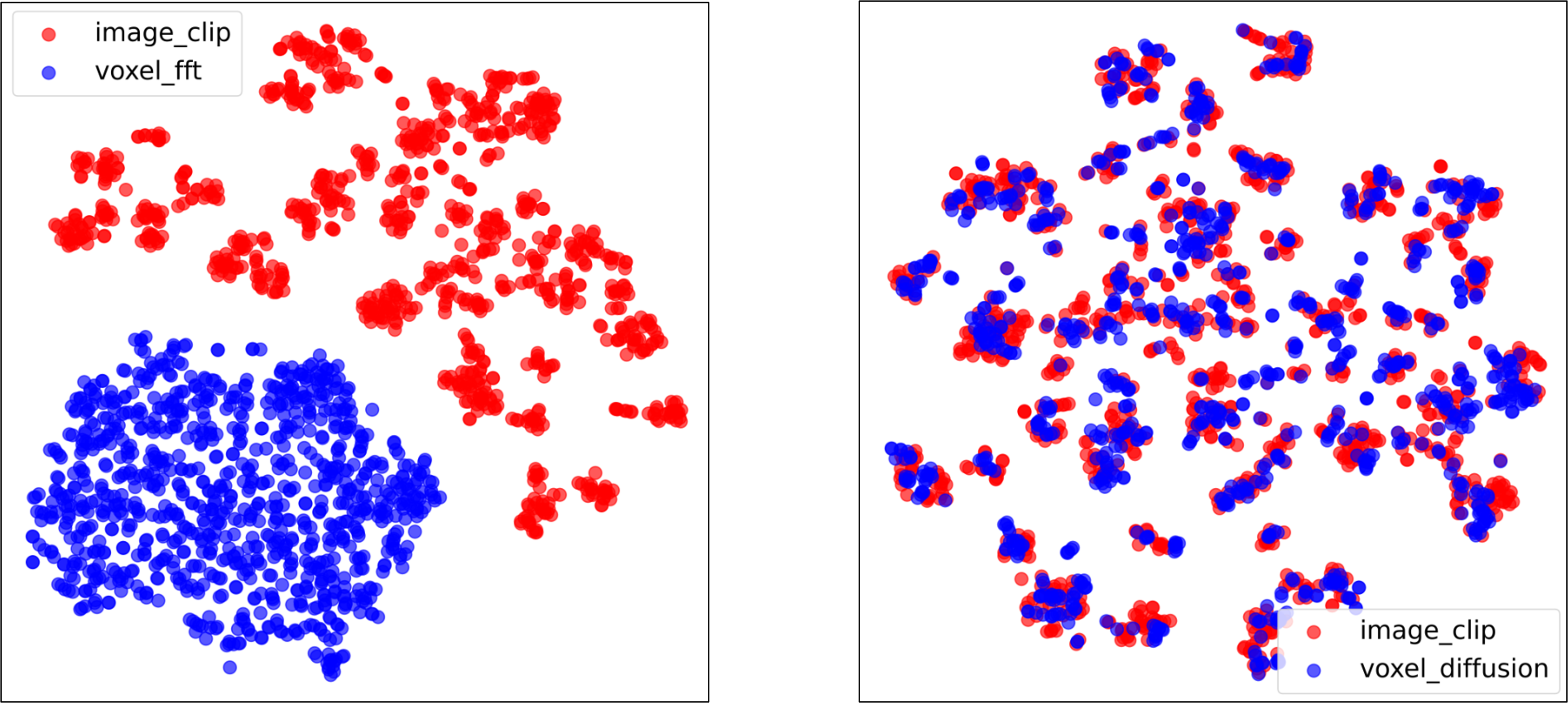
Figure 5: T-SNE of representations of 982 test fMRI voxels by diffusion projector on LAION-5B retrieval for Subject 5. The diffusion model plays a role in bringing vectors closer, enabling img2img retrieval on the LAION-5B dataset.

7 Conclusion

In this work, we propose Lite-Mind, an extremely lightweight brain representation extraction network based on Fourier transform for cross-modal fMRI-image retrieval. Our DFT Backbone is an efficient means of obtaining fine-grained representation alignment between fMRI signals and visual stimuli. With high retrieval accuracy, Lite-Mind can transform many downstream fMRI tasks into retrieval-based tasks, such as zero-shot classification. Meanwhile, Lite-Mind’s dependence on data volume and voxel values is less than that of larger models, demonstrating excellent universality across different fMRI datasets.

For future work, we should explore the relationship between different sizes of patches and brain area structures and explore the impact of cortices other than the visual cortex, such as ventral, on retrieval accuracy. In addition, versatile cross-subject models should be studied to efficiently project fMRI representations of different subjects into the same joint space or transfer from subject models with larger sample sizes to models with sparse sample sizes. At the same time, how to use an efficient model to collaboratively train multiple fMRI datasets (across subjects) is also a promising direction that can be explored in the future.

Supplementary Material

Appendix A Additional Method Details

A.1 Implementation details

Data preprocessing. We downloaded the NSD dataset from the official website and used Takagi’s code to extract nsdgenal fMRI voxels, while Takagi extracted the stream region of the NSD dataset. We noticed that MindEye scaled the fMRI voxel values in advance, while we did not. The difference in fMRI voxels input data is shown in the example in Figure 6. NSD image files come from nsd-stimuli.hdf5 file and have a unified size of $425\times 425$. We did not perform any data augmentation on the image and straightly extracted the hidden layer representation (size of $257\times 768$) of the image through CLIP ViT-L/14 for training.

Hyper-parameters. On the NSD dataset, during training DFT Backbone, the weight decay is set to 7, $\tau$ is $1/e^{8}$, $\alpha=1$, and $\beta=0$, and CLIP’s contrastive loss is unidirectional for image retrieval and fMRI retrieval. Owning to the lightweight nature of Lite-Mind, the batch size is set to 1500, and the learning rate is 1.16e-3. For Subject 1, 2, 5, 7, Pyramid is set to [512, 256, 128, 257] respectively, and the corresponding number of layers and the patch size are set to [2, 10, 2, 4] and [480, 440, 460, 450], respectively.

About LAION-5B retrieval, for DFT Backbone, the weight decay is set to 7, $\tau$ is $1/e^{8}$, while the weight decay is 6.02e-2 for diffusion projector. CLIP’s contrastive loss is unidirectional for image retrieval, $\alpha=0.5$, and $\beta=0.5$, the batch size is set to 80 and the learning rate is 1.16e-3 for DFT Backbone while 1.1e-4 for diffusion projector.

On the GOD dataset, the hyperparameters are the same as those on the NSD dataset, except for the batch size and patch size which are set to 1200 and 8 for all 5 subjects on the GOD dataset, respectively.

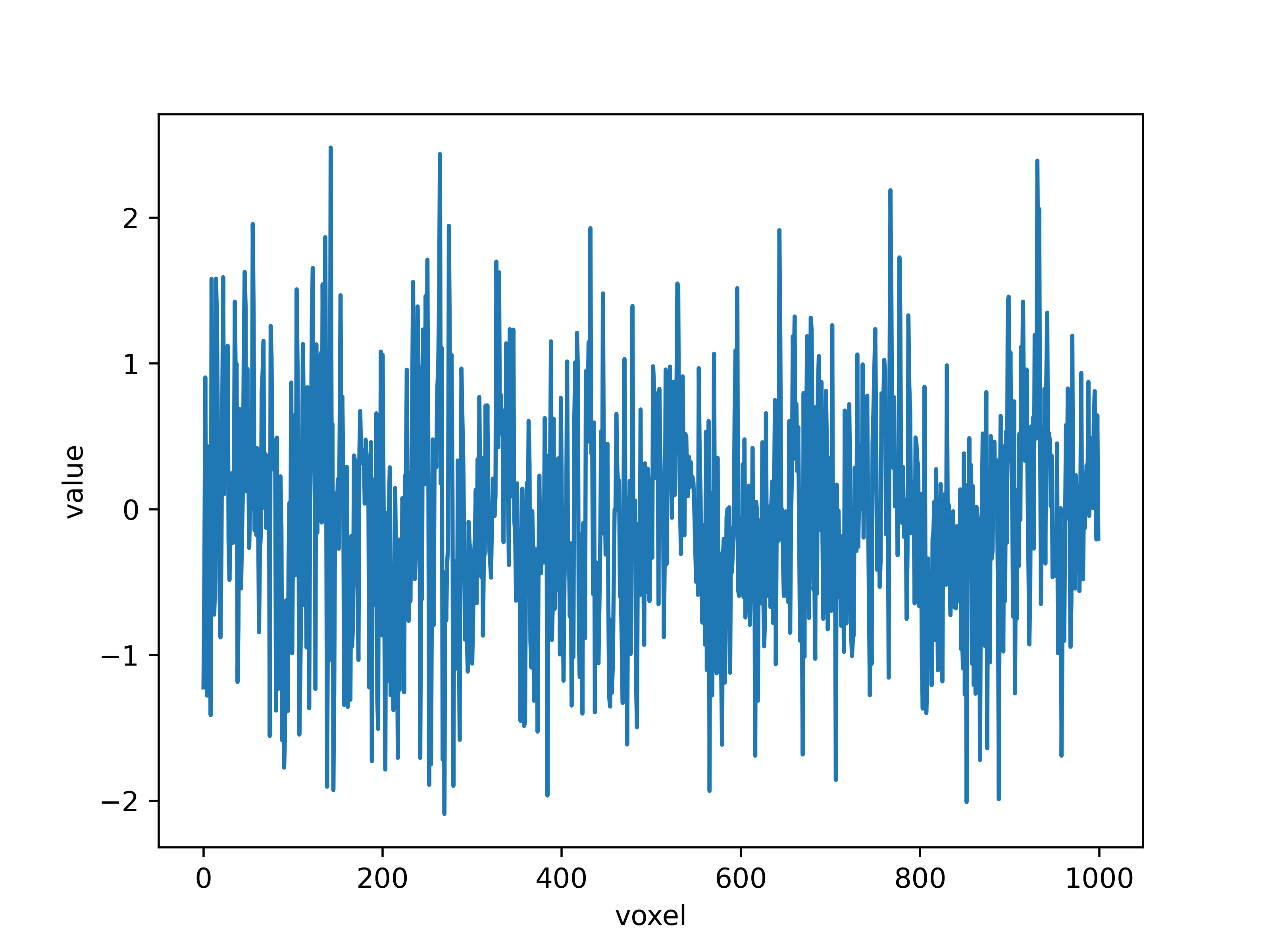
(a) MindEye

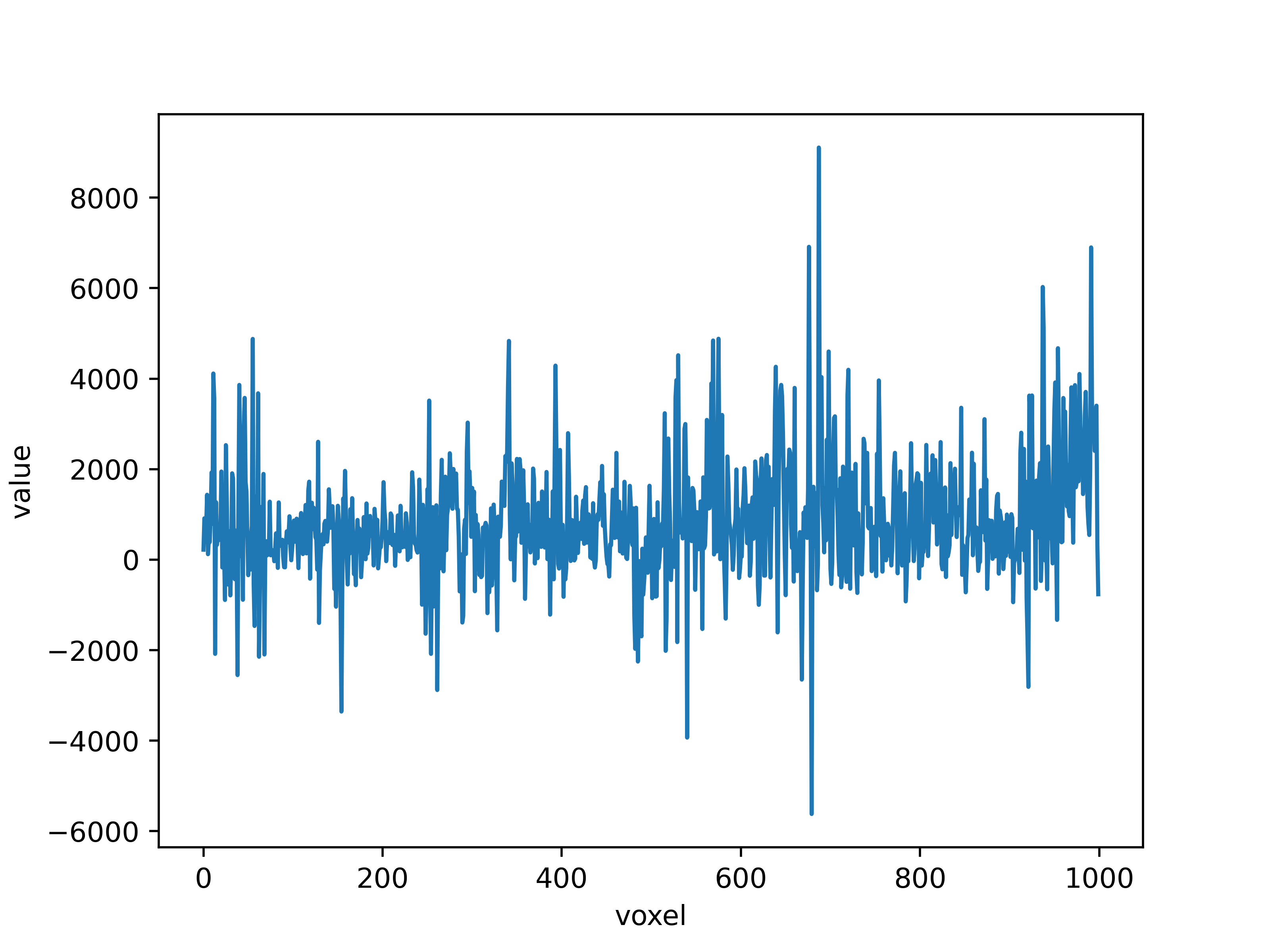
(b) Lite-Mind

Figure 6: The fMRI averaged activities of MindEye and Lite-Mind responding to the same image, respectively. The figures only visualize the activities of the first 1000 voxels for illustration.

Appendix B Additional Experiment Results

B.1 Additional Results of Retrieval

To demonstrate the applicability of our method, we also conducted experiments on three other subjects, i.e., Subject 2, Subject 5, and Subject 7, on the NSD dataset, and the experimental results are shown in Table 4. In order to control model size similarity, we did not make more targeted model adjustments for subjects with shorter voxel lengths, but instead used smaller patches. It can be seen that the retrieval accuracies of Subjects 1 and 2 are greater than 90, and the retrieval accuracies of Subjects 5 and 7 are also above 75, The results prove that DFT Backbone can efficiently work on different subjects. Note that MindEye only includes the results of the overall model in Subjects 2, 5, and 7 in its appendix, and it does not evaluate the effect of individual MLP Backbone. As a result, Table 4 does not present any evaluation results for MindEye.

Method	Voxel Length	Parameters	Retrieval
			Image$\uparrow$	Brain$\uparrow$
Lite-Mind(Subj 1)	15724	12.51M	94.3%	97.4%
Lite-Mind(Subj 2)	14278	12.49M	93.4%	98.2%
Lite-Mind(Subj 5)	13039	12.47M	80.5%	86.3%
Lite-Mind(Subj 7)	12682	12.47M	75.0%	82.3%

Table 4: Addtional retrieval performance for individual subjects on 982 test images of the NSD dataset.

Method	Low-Level				High-Level
	PixCorr$\uparrow$	SSIM$\uparrow$	Alex(2)$\uparrow$	Alex(5)$\uparrow$	Incep$\uparrow$	CLIP$\uparrow$	Eff$\downarrow$	SwAV$\downarrow$
Lite-Mind(Subject 1)	.134	.332	78.8%	88.9%	88.5%	88.8%	.730	.451
Lite-Mind(Subject 2)	.120	.328	78.0%	89.4%	86.3%	87.4%	.730	.446
Lite-Mind(Subject 5)	.123	.332	79.4%	90.0%	88.8%	89.9%	.712	.440
Lite-Mind(Subject 7)	.121	.331	78.7%	88.8%	87.8%	88.5%	.723	.448

Table 5: LAION-5B retrieval alternative reconstruction performance for the specific subject.

B.2 Additional Results of LAION-5B Retrieval

In order to better reflect the retrieval performance of Lite-Mind on LAION-5B, we presented the performance indicators of LAION-5B retrieval substitution reconstruction for other subjects, i.e., Subject 2, Subject 5, and Subject 7, in Table 5, corresponding to the average performance of subjects in Table 1(b). Similarly, the visualization results of the other subjects in Figure 7 correspond to the image samples of Subject 1 in Figure 4. Based on the comprehensive table and graph, it can be found that Lite-Mind has good generalization on all four subjects, verifying the LAION-5B retrieval ability of Lite-Mind on different subjects. Meanwhile, as shown in Figure 7, the retrieval performance of LAION-5B completely depends on the retrieval accuracy of the CLS model in the test set, such that images retrieved incorrectly in the test set may also have retrieval bias on LAION-5B, for example treating a teddy bear as an image of a cat or dog as shown in Figure 7. However, both MindEye and Lite-Mind exhibit relatively low retrieval accuracy with aligned CLS token models. In the future, it would be beneficial to explore models that improve the alignment of CLS tokens or employ more efficient methods to directly perform retrieval through hidden layers in LAION-5B.

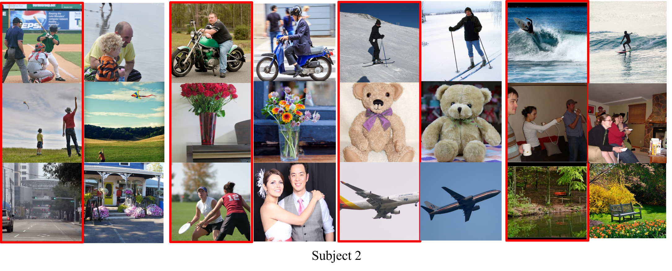
Figure 7: Addtional retrieval results corresponding to Figure 4. The left column marked by a red box in every two columns represents the original image seen by the subject, and the right column represents the image retrieved on LAION-5B.

B.3 Additional Results of Zero-shot Classification

In the main body of the paper, we only demonstrated the zero-shot classification effect of Lite-Mind on the GOD dataset. The corresponding retrieval results of each Subject are shown in the Table 6 below.

Method	Voxel Length	Parameters	Image Retrieval$\uparrow$
			top1	top5
Lite-Mind(Subj 1)	4466	15.50M	30.0%	60.0%
Lite-Mind(Subj 2)	4404	15.46M	38.0%	58.0%
Lite-Mind(Subj 3)	4643	15.64M	38.0%	72.0%
Lite-Mind(Subj 4)	4133	15.24M	42.0%	62.0%
Lite-Mind(Subj 5)	4370	15.43M	26.0%	54.0%

Table 6: Retrieval performance on the GOD dataset.

B.4 Additional Ablations

In this section, we delved into the dependence of Lite-Mind on data volume and feature length on the NSD dataset and explored the specific impact of different cerebral cortexes on retrieval accuracy, not just nsdgenal. All the experimental results on the NSD dataset are derived from Subject 1, with a retrieving pool size of 300.

B.4.1 Retrieval with varying dataset size

In order to better investigate the versatile representation of DFT Backbone, we conducted data volume experiments on the NSD dataset, as shown in Table 7. Among them, All data corresponds to all trials of every single Subject on the NSD dataset, and 24890 fMRI-image pairs are used for training; Half data refers to randomly removing half of the training data; 2-session refers to using only 1500 randomly selected fMRI-image pairs for training, which corresponds to the two scan sessions of the fMRI experiment. In the table, we report the results of MLP Backbone and diffusion models for MindEye. The experimental results indicate that even in the same NSD dataset, the dependence of Lite-Mind on the number of training samples is smaller than that of MindEye. This also proves that the lightweight model has a wider applicability, i.e., versatility.

Method	Parameters	Retrieval
		Image$\uparrow$	Brain$\uparrow$
All Data(MindEye)	3B	97.2%	94.7%
Half Data(MindEye)	3B	77.5%	60.8%
2-Sessions(MindEye)	3B	17.9%	12.0%
All Data(Lite-Mind)	12.5M	94.3%	97.4%
Half Data(Lite-Mind)	12.5M	83.4%	91.9%
2-Sessions(Lite-Mind)	12.5M	11.9%	14.1%

Table 7: Retrieval performance with varying dataset size for Subject 1 on the NSD dataset.

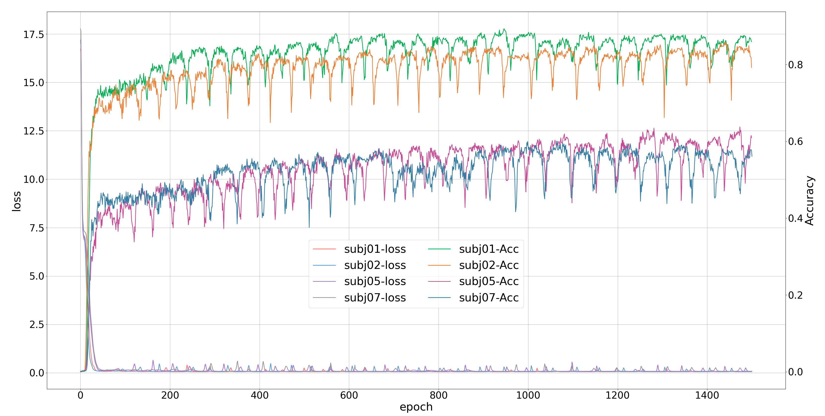
Figure 8: Lite-Mind’s training loss curve and testing accuracy curve for Suject 1, 2, 5, 7 on the NSD dataset. The testing accuracy is calculated based on a retrieval pool of size 982.

B.4.2 Retrieval with varying representation sizes

We conducted additional experiments to verify the impact of representation dimensions on retrieval accuracy, as shown in Table 8. Among them, two different CLIP models (i.e., CLIP ViT/B-32 and CLIP ViT/L-14) were used to extract image representation, with a total of four representation dimensions, by CLS token and the last hidden layer, respectively. From the results, it can be seen that the retrieval accuracy of Lite-Mind is higher when the representation dimension of the image is longer and the representation of the image is richer. The results verify that the fine-grained alignment we mentioned in the main text comes from the rich representation of the image, rather than the fMRI voxel value fully connected heavy MLP Backbone.

Method	Representation	Parameters	Retrieval
	Dimension		Image$\uparrow$	Brain$\uparrow$
ViT-B/32 CLS	512	6.7M	57.5%	61.8%
ViT-L/14 CLS	768	6.7M	60.3%	64.2%
ViT-B/32 Hidden	50×512	10.4M	91.1%	96.5%
ViT-L/14 Hidden	257×768	12.5M	94.3%	97.4%

Table 8: Retrieval performance with different CLIP representation for Subject 1 on the NSD dataset.

B.4.3 Cerebral cortex

In order to explore the impact of different cortical regions on retrieval accuracy, we used Takagi’s method to extract the stream region of the NSD dataset, covering the visual cortex of nsdgenal, and separately trained the retrieval model for each cortex (early, lateral, parietal, ventral). As shown in Table 9, it can be observed that the early visual cortex has the greatest impact on retrieval accuracy, although with only 5917 voxels Lite-Mind can still achieve retrieval accuracy of 85.0% and 93.4%, which is consistent with Takagi’s research. They believe that visual stimuli are almost dominated by the early visual cortex and indicate that nsdgenal still has a low signal-to-noise ratio, proving that fully connected backbones are unnecessary. Interestingly, for other cortical regions, both lateral and ventral have a good impact on retrieval accuracy, while parietal shows little impact. The findings indicate the necessity of further research on whether the accuracy improvement is related to the longer voxel length of these two regions.

Region	Voxel Length	Parameters	Retrieval
			Image$\uparrow$	Brain$\uparrow$
early	5917	12.4M	85.0%	93.4%
lateral	7799	12.4M	26.9%	29.0%
parietal	3548	12.3M	9.6%	11.2%
ventral	7604	12.3M	18.1%	22.4%

Table 9: Retrieval performance with different cerebral cortex for Subject 1 on the NSD dataset.

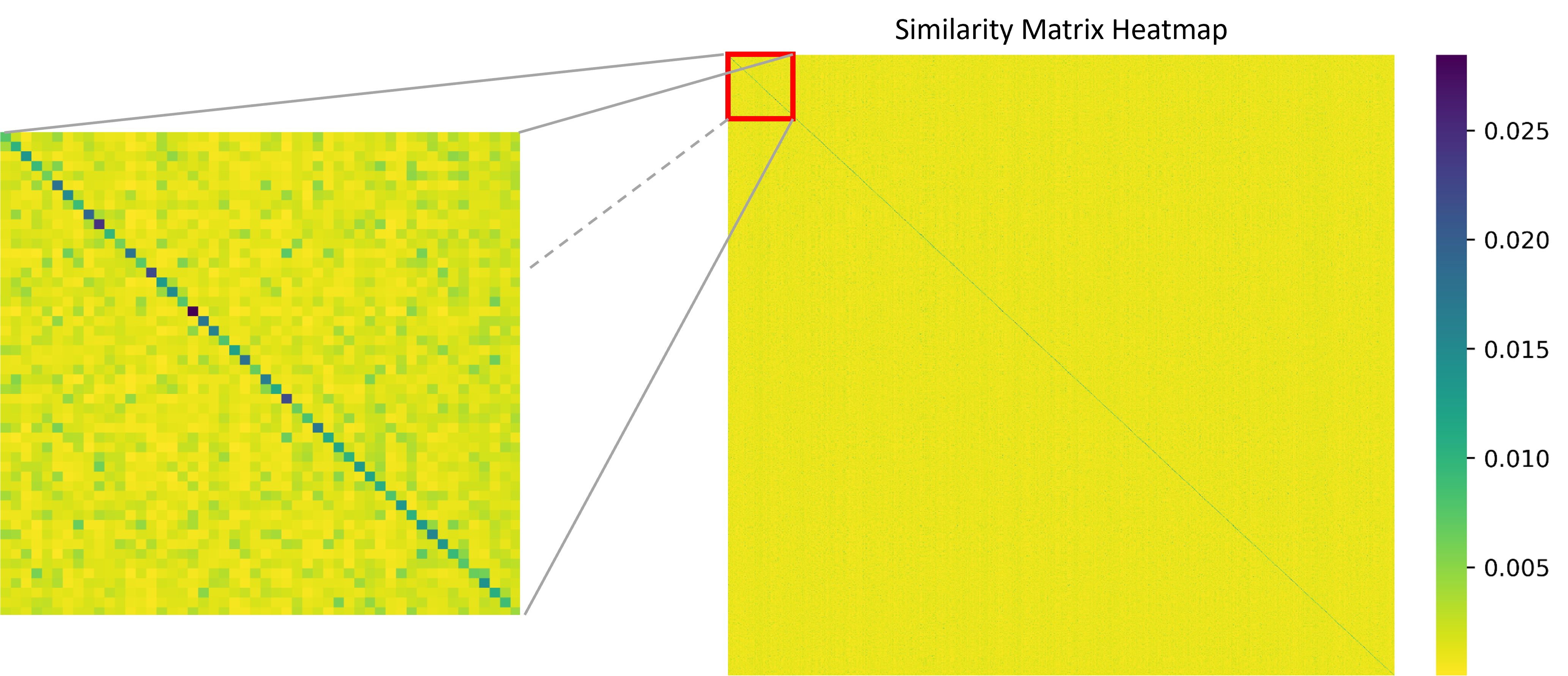
Figure 9: Lite-Mind’s retrieval heatmap on the NSD dataset for Subject 1. The larger figure on the right represents 982 × 982’s heatmap, and the smaller figure on the left represents the 50 × 50 subgraph.

Appendix C Additional Visualization

C.1 Training Curve

We visualized the training process of all four subjects on the NSD dataset in Figure 8. As the training epochs increased, the loss of the training set rapidly decreased, while the accuracy of the test set rapidly increased and then showed a slow upward trend. Accuracy refers to the hit rate of correct retrieval from 982 test set images.

C.2 Retrieval Heatmap

We visualized the retrieval heatmap for Subject 1 on all 982 test images of the NSD dataset in Figure 9. It can be observed that the similarity is highest on the diagonal, and the color of the retrieved heat map is darker. It shows that Lite-Mind has effectively retrieved corresponding images, even if there are many similar images in the test set, which verifies the fine-grained ability of Lite-Mind.

C.3 Visualization in Frequency Domain

We visualized the weights of different patches in different layers of filters, as shown in Figure 10 and 11. Visualization is divided into the real part (left) and imaginary part (right) of filter weights. It can be observed that different channels have varying degrees of attention to different patches, and the frequency domain better captures this characteristic. Interestingly, the weight of the imaginary part for the first and last patches is almost always 0, indicating that the noise is distributed in these two patches.

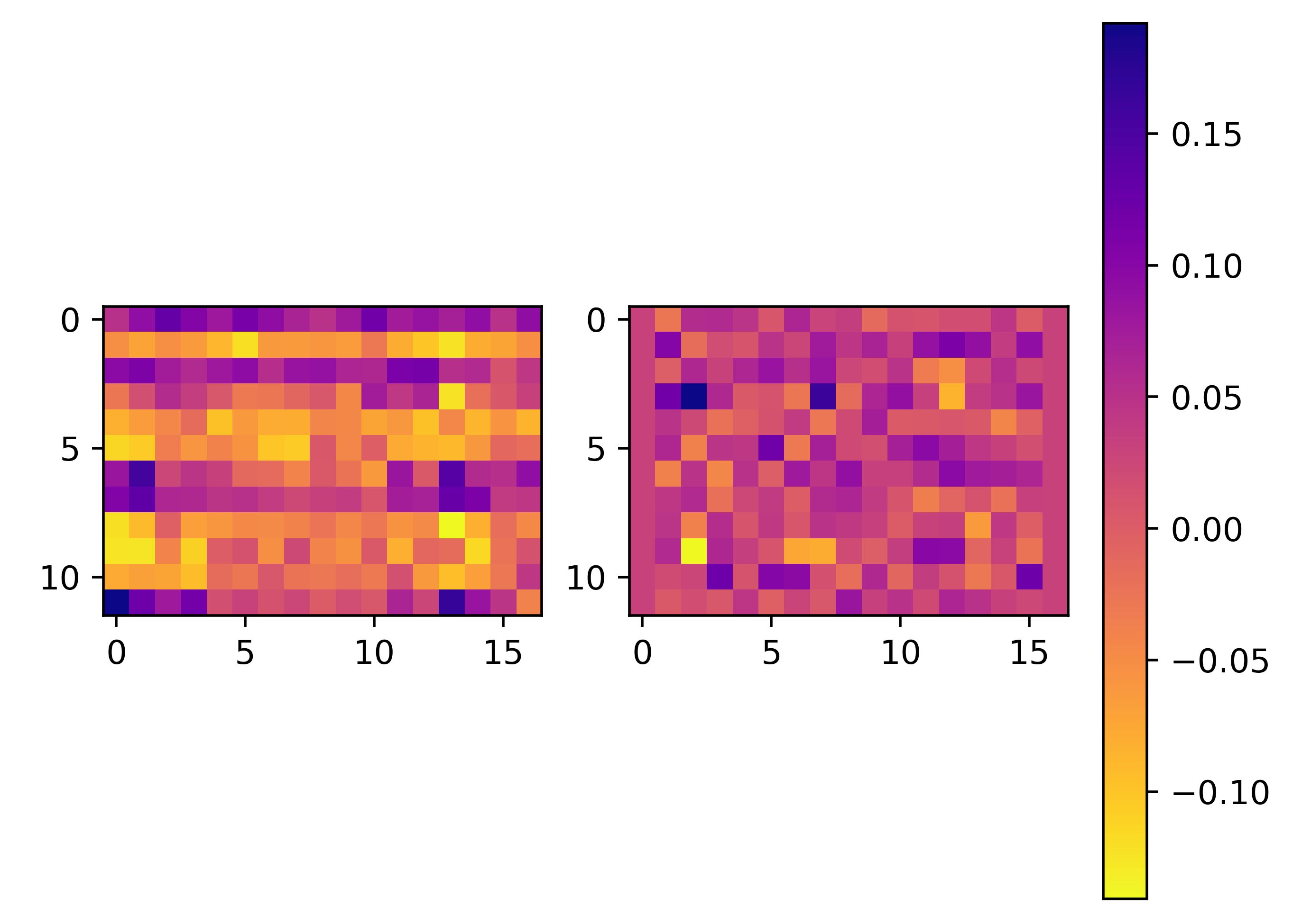
(a) The real part and imaginary of patch weights for CLS token channel.

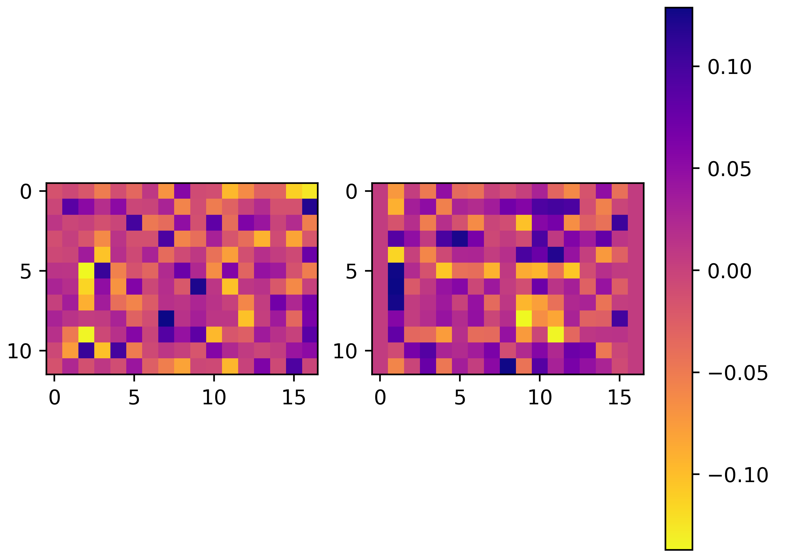
(b) The real part and imaginary of patch weights for 140th channel.

Figure 10: Weights visualization for DFT Backbone of $257\times 768$ representation length.

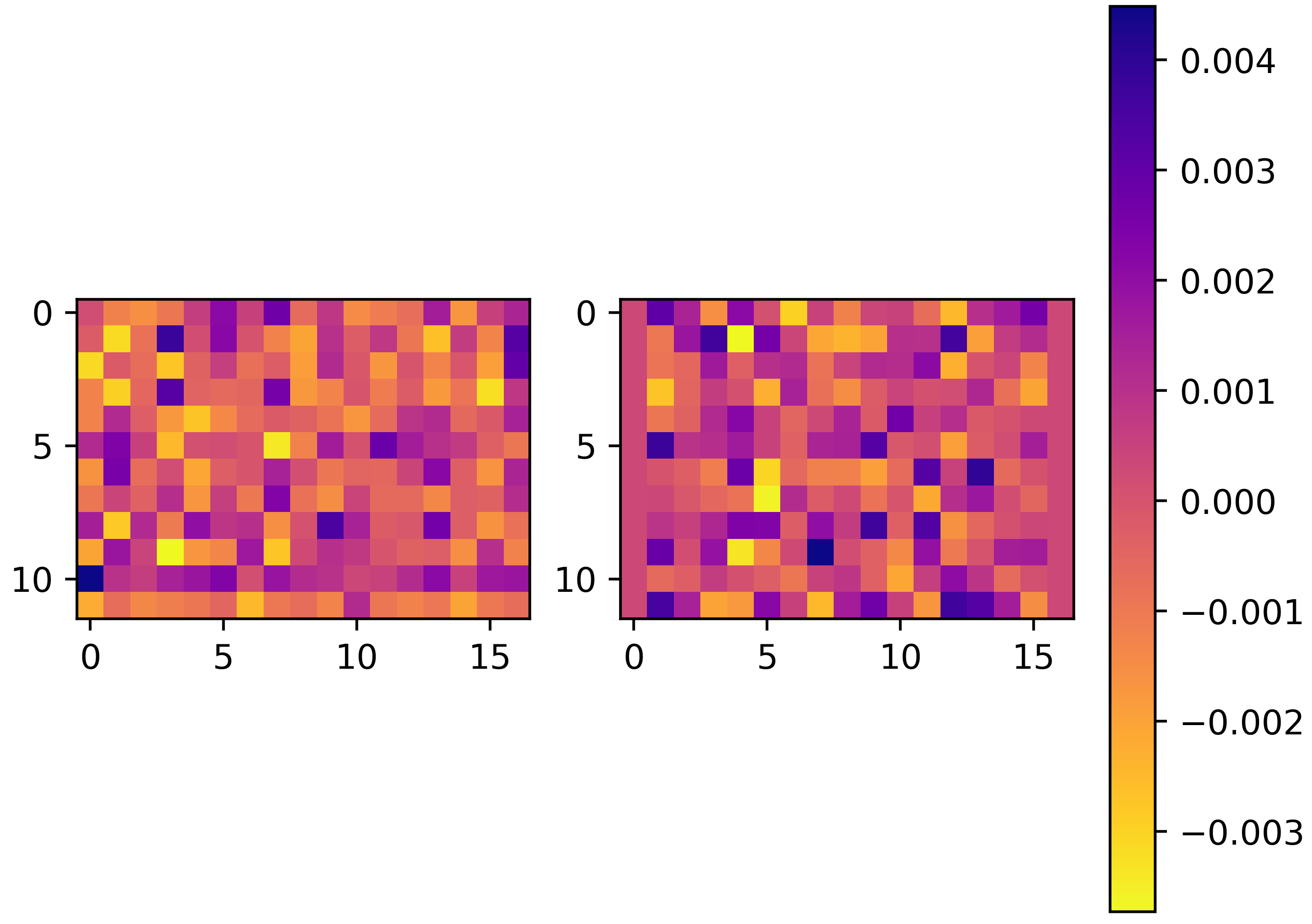
(a) The real part and imaginary of patch weights for the 1st channel.

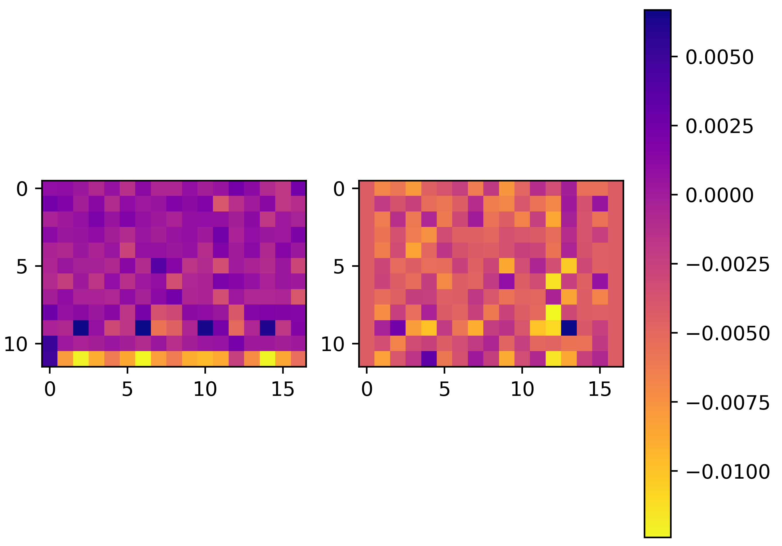
(b) The real part and imaginary of patch weights for the 60th channel.

Figure 11: Weights visualization for DFT Backbone of 768 representation length.

C.4 Information Alignment

We visualized the T-SNE plot between the voxel embeddings output by DFT Backbone and the image embeddings of frozen CLIP as the accuracy of the test set improved, as shown in Figure 12. We can observe that as the training progresses, the retrieval accuracy of the test set improves, and the shape of voxel embeddings tends to be closer to image embeddings, indicating the success of contrastive learning.

Appendix D Efficiency Discussion

D.1 Theoretical Analysis.

Theorem. Suppose that H is the representation of raw fMRI voxel patches and $\mathcal{H}$ is the corresponding frequency components of the spectrum, then the energy of a voxel patch series in the spatial domain is equal to the energy of its representation in the frequency domain. Formally, we can express this with the above notations:

$$\int_{-\infty}^{\infty}{|\textbf{H}(v)|}^{2}\,\mathrm{d}v=\int_{-\infty}^{\infty}{|\mathcal{H}(f)|}^{2}\,\mathrm{d}f$$ (7)

Where $\mathcal{H}(f)=\int_{-\infty}^{\infty}{|\textbf{H}(v)|}e^{-j2{\pi}fv}\,\mathrm{d}v$, $v$ is the spatial/channel dimension, $f$ is the frequency dimension.

Proof.

Given the representation of raw voxel patch series $H\in\mathbb{R}^{C\times N}$, let us consider performing integration in either the $C$ dimension (channel dimension) or the $N$ dimension (spatial dimension), denoted as the integral over $v$, then

$$\int_{-\infty}^{\infty}{|\textbf{H}(v)|}^{2}\,\mathrm{d}v=\int_{-\infty}^{\infty}{\textbf{H}(v)}{\textbf{H}^{*}(v)}\,\mathrm{d}v$$ (8)

where $\textbf{H}^{*}(v)$ is the conjugate of $\textbf{H}(v)$. According to IDFT, $\textbf{H}^{*}(v)=\int_{-\infty}^{\infty}{\mathcal{H}^{*}(f)}e^{-j2{\pi}fv}\,\mathrm{d}f$, we can obtain

$$\int_{-\infty}^{\infty}{|\textbf{H}(v)|}^{2}\,\mathrm{d}v =\int_{-\infty}^{\infty}{\textbf{H}(v)}[\int_{-\infty}^{\infty}{\mathcal{H}^{*}(f)}e^{-j2{\pi}fv}\,\mathrm{d}f]\,\mathrm{d}v$$ (9)

$$=\int_{-\infty}^{\infty}{\mathcal{H}}^{*}(f)[\int_{-\infty}^{\infty}{|\textbf{H}(v)|}e^{-j2{\pi}fv}\,\mathrm{d}v]\,\mathrm{d}f$$

$$=\int_{-\infty}^{\infty}{\mathcal{H}^{*}(f)}{\mathcal{H}(f)}\,\mathrm{d}f$$

$$=\int_{-\infty}^{\infty}{|\mathcal{H}(f)|}^{2}\,\mathrm{d}f$$

Proved. ∎

Therefore, the energy of a voxel patch series in the spatial domain is equal to the energy of its representation in the frequency domain.

Complexity Analysis. For a fMRI voxel with a length of $m$, we divide it into $n$ $l$-length patches ($m=nl$) with $C$ channel numbers. Assuming $L_{1}$ and $L_{2}$ are the layer depths of MLP and DFT respectively, the middle layer dimension of MLP is $D_{1}$, and the alignment representation dimension is $N\times D_{2}$, where $N$ is the number of the last hidden layer of CLIP. The time complexity of MLP Backbone is $O(mD_{1}+L_{1}D_{1}^{2}+ND_{1}D_{2})$. For DFT Backobone, the time complexity of patchfy is $O(mC)$, and the time complexity of DFT, IDFT, and filtering for each layer is $O(2nC\operatorname{log}n+nC)$. The time complexity of each layer’s tiny MLP is $O(8nC^{2})$. Thus the time complexity of the entire DFT Backbone is:

$$O(mC+L_{2}(2nC\operatorname{log}n+nC+8nC^{2})+nD_{2})$$ (10)

$$=O(mC+nC\operatorname{log}nL_{2}+nC^{2}L_{2}+nD_{2})$$

Quantitative analysis algorithm complexity for DFT Backbone is shown in Table 10.

Model	FLOPs(G)	Parameters	Image Retrieval	Brain Retrieval
MindEye	5.66	996M	88.8%	84.9%
Pyramid-18	0.80	12.5M	94.3%	97.4%
DFT-18	0.63	9.9M	91.8%	97.3%
DFT-12	0.43	6.6M	91.0%	97.2%
DFT-6	0.22	3.4M	90.6%	97.2%
DFT-1	0.05	0.7M	83.5%	94.0%
DFT-0	0.02	0.2M	65.8%	74.7%

Table 10: Quantitative complexity analysis for DFT Backbone with different layers and MLP Backbone+Projector for MindEye.

Figure 12: T-SNE visualization between the voxel embeddings output by DFT Backbone and the image embedding of frozen CLIP. Accuracy in the title refers to the hit rate of correct retrieval from 982 test set images and the blue dots represent voxel embeddings.

References

- Allen et al. [2022] Emily J Allen, Ghislain St-Yves, Yihan Wu, Jesse L Breedlove, Jacob S Prince, Logan T Dowdle, Matthias Nau, Brad Caron, Franco Pestilli, Ian Charest, et al. A massive 7t fmri dataset to bridge cognitive neuroscience and artificial intelligence. Nature neuroscience, 25(1):116–126, 2022.
- Beaumont [2022] Romain Beaumont. Clip retrieval: Easily compute clip embeddings and build a clip retrieval system with them, 2022.
- Cao et al. [2020] Defu Cao, Yujing Wang, Juanyong Duan, Ce Zhang, Xia Zhu, Congrui Huang, Yunhai Tong, Bixiong Xu, Jing Bai, Jie Tong, et al. Spectral temporal graph neural network for multivariate time-series forecasting. Advances in neural information processing systems, 33:17766–17778, 2020.
- Caron et al. [2020] Mathilde Caron, Ishan Misra, Julien Mairal, Priya Goyal, Piotr Bojanowski, and Armand Joulin. Unsupervised learning of visual features by contrasting cluster assignments. Advances in neural information processing systems, 33:9912–9924, 2020.
- Chen et al. [2023] Zijiao Chen, Jiaxin Qing, Tiange Xiang, Wan Lin Yue, and Juan Helen Zhou. Seeing beyond the brain: Conditional diffusion model with sparse masked modeling for vision decoding. In Proceedings of the IEEE/CVF Conference on Computer Vision and Pattern Recognition, pages 22710–22720, 2023.
- Deng et al. [2009] Jia Deng, Wei Dong, Richard Socher, Li-Jia Li, Kai Li, and Li Fei-Fei. Imagenet: A large-scale hierarchical image database. In 2009 IEEE conference on computer vision and pattern recognition, pages 248–255. Ieee, 2009.
- Du et al. [2023] Changde Du, Kaicheng Fu, Jinpeng Li, and Huiguang He. Decoding visual neural representations by multimodal learning of brain-visual-linguistic features. IEEE Transactions on Pattern Analysis and Machine Intelligence, 2023.
- Ehrlich and Davis [2019] Max Ehrlich and Larry S Davis. Deep residual learning in the jpeg transform domain. In Proceedings of the IEEE/CVF international conference on computer vision, pages 3484–3493, 2019.
- Emmanuele et al. [2021] Chersoni Emmanuele, Santus Enrico, Huang Chu-Ren, Alessandro Lenci, et al. Decoding word embeddings with brain-based semantic features. Computational Linguistics, 47(3):663–698, 2021.
- Gu et al. [2022] Zijin Gu, Keith Jamison, Amy Kuceyeski, and Mert Sabuncu. Decoding natural image stimuli from fmri data with a surface-based convolutional network. arXiv preprint arXiv:2212.02409, 2022.
- Gueguen et al. [2018] Lionel Gueguen, Alex Sergeev, Ben Kadlec, Rosanne Liu, and Jason Yosinski. Faster neural networks straight from jpeg. Advances in Neural Information Processing Systems, 31, 2018.
- Guibas et al. [2021] John Guibas, Morteza Mardani, Zongyi Li, Andrew Tao, Anima Anandkumar, and Bryan Catanzaro. Adaptive fourier neural operators: Efficient token mixers for transformers. arXiv preprint arXiv:2111.13587, 2021.
- Horikawa and Kamitani [2017] Tomoyasu Horikawa and Yukiyasu Kamitani. Generic decoding of seen and imagined objects using hierarchical visual features. Nature communications, 8(1):15037, 2017.
- Kamitani and Tong [2005] Yukiyasu Kamitani and Frank Tong. Decoding the visual and subjective contents of the human brain. Nature neuroscience, 8(5):679–685, 2005.
- Kewenig et al. [2023] Viktor Kewenig, Christopher Edwards, Quitterie Lacome DEstalenx, Akilles Rechardt, Jeremy I Skipper, and Gabriella Vigliocco. Evidence of human-like visual-linguistic integration in multimodal large language models during predictive language processing. arXiv preprint arXiv:2308.06035, 2023.
- Koç and Koç [2022] Emirhan Koç and Aykut Koç. Fractional fourier transform in time series prediction. IEEE Signal Processing Letters, 29:2542–2546, 2022.
- Lange et al. [2021] Henning Lange, Steven L Brunton, and J Nathan Kutz. From fourier to koopman: Spectral methods for long-term time series prediction. The Journal of Machine Learning Research, 22(1):1881–1918, 2021.
- Lee-Thorp et al. [2021] James Lee-Thorp, Joshua Ainslie, Ilya Eckstein, and Santiago Ontanon. Fnet: Mixing tokens with fourier transforms. arXiv preprint arXiv:2105.03824, 2021.
- Lin et al. [2022] Sikun Lin, Thomas Sprague, and Ambuj K Singh. Mind reader: Reconstructing complex images from brain activities. Advances in Neural Information Processing Systems, 35:29624–29636, 2022.
- Linden [2021] David Linden. Section 3 - introduction. In fMRI Neurofeedback, pages 161–169. Academic Press, 2021.
- Liu et al. [2023] Yulong Liu, Yongqiang Ma, Wei Zhou, Guibo Zhu, and Nanning Zheng. Brainclip: Bridging brain and visual-linguistic representation via clip for generic natural visual stimulus decoding from fmri. arXiv preprint arXiv:2302.12971, 2023.
- Loshchilov and Hutter [2017] Ilya Loshchilov and Frank Hutter. Decoupled weight decay regularization. arXiv preprint arXiv:1711.05101, 2017.
- Mai and Zhang [2023] Weijian Mai and Zhijun Zhang. Unibrain: Unify image reconstruction and captioning all in one diffusion model from human brain activity. arXiv preprint arXiv:2308.07428, 2023.
- Naselaris et al. [2011] Thomas Naselaris, Kendrick N Kay, Shinji Nishimoto, and Jack L Gallant. Encoding and decoding in fmri. Neuroimage, 56(2):400–410, 2011.
- Ozcelik and VanRullen [2023] Furkan Ozcelik and Rufin VanRullen. Brain-diffuser: Natural scene reconstruction from fmri signals using generative latent diffusion. arXiv preprint arXiv:2303.05334, 2023.
- Palazzo et al. [2020] Simone Palazzo, Concetto Spampinato, Isaak Kavasidis, Daniela Giordano, Joseph Schmidt, and Mubarak Shah. Decoding brain representations by multimodal learning of neural activity and visual features. IEEE Transactions on Pattern Analysis and Machine Intelligence, 43(11):3833–3849, 2020.
- Pereira et al. [2018] Francisco Pereira, Bin Lou, Brianna Pritchett, Samuel Ritter, Samuel J Gershman, Nancy Kanwisher, Matthew Botvinick, and Evelina Fedorenko. Toward a universal decoder of linguistic meaning from brain activation. Nature communications, 9(1):963, 2018.
- Radford et al. [2021] Alec Radford, Jong Wook Kim, Chris Hallacy, Aditya Ramesh, Gabriel Goh, Sandhini Agarwal, Girish Sastry, Amanda Askell, Pamela Mishkin, Jack Clark, et al. Learning transferable visual models from natural language supervision. In International conference on machine learning, pages 8748–8763. PMLR, 2021.
- Ramesh et al. [2022] Aditya Ramesh, Prafulla Dhariwal, Alex Nichol, Casey Chu, and Mark Chen. Hierarchical text-conditional image generation with clip latents. arXiv preprint arXiv:2204.06125, 2022.
- Rao et al. [2021] Yongming Rao, Wenliang Zhao, Zheng Zhu, Jiwen Lu, and Jie Zhou. Global filter networks for image classification. Advances in neural information processing systems, 34:980–993, 2021.
- Schonfeld et al. [2019] Edgar Schonfeld, Sayna Ebrahimi, Samarth Sinha, Trevor Darrell, and Zeynep Akata. Generalized zero-and few-shot learning via aligned variational autoencoders. In Proceedings of the IEEE/CVF conference on computer vision and pattern recognition, pages 8247–8255, 2019.
- Schuhmann et al. [2022] Christoph Schuhmann, Romain Beaumont, Richard Vencu, Cade Gordon, Ross Wightman, Mehdi Cherti, Theo Coombes, Aarush Katta, Clayton Mullis, Mitchell Wortsman, et al. Laion-5b: An open large-scale dataset for training next generation image-text models. Advances in Neural Information Processing Systems, 35:25278–25294, 2022.
- Scotti et al. [2023] Paul S Scotti, Atmadeep Banerjee, Jimmie Goode, Stepan Shabalin, Alex Nguyen, Ethan Cohen, Aidan J Dempster, Nathalie Verlinde, Elad Yundler, David Weisberg, et al. Reconstructing the mind’s eye: fmri-to-image with contrastive learning and diffusion priors. arXiv preprint arXiv:2305.18274, 2023.
- Shen et al. [2019] Guohua Shen, Tomoyasu Horikawa, Kei Majima, and Yukiyasu Kamitani. Deep image reconstruction from human brain activity. PLoS computational biology, 15(1):e1006633, 2019.
- Shi et al. [2019] Yuge Shi, Brooks Paige, Philip Torr, et al. Variational mixture-of-experts autoencoders for multi-modal deep generative models. Advances in neural information processing systems, 32, 2019.
- Takagi and Nishimoto [2023] Yu Takagi and Shinji Nishimoto. High-resolution image reconstruction with latent diffusion models from human brain activity. In Proceedings of the IEEE/CVF Conference on Computer Vision and Pattern Recognition, pages 14453–14463, 2023.
- [37] Mingxing Tan and V Le Quoc. Efficientnet: Rethinking model scaling for convolutional neural networks, september 2020. arXiv preprint arXiv:1905.11946.
- Wang et al. [2023] S Wang, K Yi, Q Zhang, W Fan, C Wang, H He, D Lian, L Cao, and Z Niu. Frequency-domain mlps are more effective learners in time series forecasting. In 37th Conference on Neural Information Processing Systems (NeurIPS 2023), 2023.
- Wang et al. [2004] Zhou Wang, Alan C Bovik, Hamid R Sheikh, and Eero P Simoncelli. Image quality assessment: from error visibility to structural similarity. IEEE transactions on image processing, 13(4):600–612, 2004.
- Wu and Goodman [2018] Mike Wu and Noah Goodman. Multimodal generative models for scalable weakly-supervised learning. Advances in neural information processing systems, 31, 2018.
- Xu et al. [2020] Kai Xu, Minghai Qin, Fei Sun, Yuhao Wang, Yen-Kuang Chen, and Fengbo Ren. Learning in the frequency domain. In Proceedings of the IEEE/CVF conference on computer vision and pattern recognition, pages 1740–1749, 2020.
- Yang and Hong [2022] Ling Yang and Shenda Hong. Unsupervised time-series representation learning with iterative bilinear temporal-spectral fusion. In International Conference on Machine Learning, pages 25038–25054. PMLR, 2022.
- Yang and Soatto [2020] Yanchao Yang and Stefano Soatto. Fda: Fourier domain adaptation for semantic segmentation. In Proceedings of the IEEE/CVF conference on computer vision and pattern recognition, pages 4085–4095, 2020.
- Zou et al. [2022] Shuxian Zou, Shaonan Wang, Jiajun Zhang, and Chengqing Zong. Cross-modal cloze task: A new task to brain-to-word decoding. In Findings of the Association for Computational Linguistics: ACL 2022, pages 648–657, 2022.