-percolation with a random
Abstract.
In -percolation, we start with an Erdős–Rényi graph and then iteratively add edges that complete copies of . The process percolates if all edges missing from are eventually added. We find the critical threshold when is uniformly random, solving a problem of Balogh, Bollobás and Morris.
Key words and phrases:
bootstrap percolation, cellular automaton, critical threshold, phase transition, random graph, weak saturation2010 Mathematics Subject Classification:
05C35, 05C80, 05C99, 60K35, 68Q801. Introduction
Following Balogh, Bollobás and Morris [1], we fix a graph , and begin with an Erdős–Rényi graph . Then, for , we obtain from by adding every edge that creates a new copy of . We let denote the graph containing all eventually added edges. When , we say that the process -percolates, or equivalently, in the terminology of Bollobás [4], that is weakly -saturated.
-percolation generalizes bootstrap percolation [7, 5], which is one of the most well-studied of all cellular automata [8, 9]. Such processes model evolving networks, in which sites update their status according to the behavior of their neighbors. Although the dynamics are local, they can lead to global behavior, emulating various real-world phenomena of interest, such as tipping points, super-spreading, self-organization and collective decision-making.
The critical -percolation threshold is defined to be the point
at which becomes likely to -percolate. Problem 1 in [1] asks for
for every graph . Finding corresponds to locating up to poly-logarithmic factors. The authors state that “Problem 1 is likely to be hard.” Indeed, e.g., even the cases remain open, for all , see Bidgoli et al. [3].
In this note, we answer Problem 1 for random graphs . We find that typically , where
is the adjusted edge per vertex ratio in [1], for graphs with vertices and edges. We recall that Theorem 1 in [1] shows that for cliques. This corresponds to the case in the following result, which, in some sense, shows that is “stable.”
Theorem 1.
Fix . Then, with high probability, as , we have that .
The case answers Problem 6 in [1], that asks for “bounds on which hold with high probability as .” We find that , except with exponentially small probability. In particular, this holds, almost surely, for all large , by the Borel–Cantelli lemma. Note that is uniformly random (from the set of simple graphs on vertices). In this sense, we find for “most” graphs .
In fact, our proof works for , for some sufficiently large constant . See Section 3.1 below for more on this.
In closing, we note that it is natural to ask about growing with . For instance, when , in which case appears to be the region of interest.
1.1. Acknowledgments
ZB is supported by the ERC Consolidator Grant 772466 “NOISE”. GK is supported by the Royal Commission for the Exhibition of 1851.
2. Background
As defined in [1], a graph is balanced if
| (1) |
for all subgraphs with . Otherwise, we call unbalanced. In [1], it is shown that for all balanced . A sharper upper bound (on ) is proved in [2] for strictly balanced graphs , which satisfy the above condition, with replaced by . Specifically, it is shown that for all such , replacing with a constant.
On the other hand, in [2] it is shown that for all , with and minimum degree , where
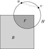
minimizing over all subgraphs with . The quantity is related to the “cost” of adding an edge, via the -percolation dynamics, as depicted in Figure 1.
As observed in [2], we have that in general, and if and only if is balanced. Moreover, when is balanced, single edges (when ) attain the minimum . When is strictly balanced, these are the only minimizers.
3. Proof
To prove Theorem 1, we show that is (strictly) balanced, with high probability. By the results from [1, 2] discussed above, the result follows.
Let us give some intuition for why random graphs , with sufficiently large edge probability , are likely to be balanced. If (1) fails for some , then the edge density of is larger than that of . For instance, if includes all but vertices, then the number of edges between these vertices and is less than (roughly) times half the average degree in . By the law of large numbers (when is large) this large deviation event is most likely to occur when , and even then, it is quite unlikely.
We will use the following, standard Chernoff tail estimates. Recall that if is binomial with mean then, for ,
| (2) |
On the other hand, for ,
| (3) |
Proposition 2.
Suppose that , for some sufficiently large constant . Then, almost surely, is strictly balanced, for all large . In particular, , for all large .
Proof.
If is not strictly balanced, then there is a subset of size , such that
| (4) |
where is the number of edges in with both endpoints in . Let be the number of all other edges in , with at most one endpoint in . For any given , the random variables and are independent. Since
(4) implies that
| (5) |
Using the Chernoff bounds (2) and (3), we will estimate the probability that (5) occurs for some of size . Note that
| (6) |
Therefore, if then, in order for (5) to hold, we would require , where
| (7) |
Let denote the probability that and take such values. (We assume throughout, since clearly the right hand side of (4) will be positive, with high probability.)
Case 1. First, we consider the case that . By (2) and (6), for any given , it follows that and take such values with probability at most , for some , where
Note that is convex and minimized at , at which point . Therefore, when ,
| (8) |
for some .
Case 2. Next, we consider . We claim that
| (9) |
for some . We will consider the cases that is smaller/larger than separately. In the former case, we consider only the large deviation by , and in the latter case, only the deviation by .
Case 2a. If , then consider the event . By (3) and (6), this occurs with probability at most , for some . Therefore (9) holds in this case.
Case 2b. If , then consider the event , with as in (7). Since , we have . By (2) and (6), this occurs with probability at most , for some . Then, since , we find, once again, that (9) holds.
Finally, we take a union bound, summing over all relevant values for the size of . For each such , there are possible values of . Therefore, combining (8) and (9) above, we find that (5) holds for some such with probability at most , for some . This is for , for large , in which case is strictly balanced with high probability. Furthermore, for large , this probability is summable. Therefore, by the Borel–Cantelli lemma, almost surely, we have that , for all large . ∎
3.1. Smaller
For ease of exposition (and since, in our view, is the most interesting case) we have not pursued the smallest possible constant in the proof above. However, we expect that more technical arguments can show that, with high probability, is balanced, and so , provided that with .
Let us give some brief intuition in this direction. Recall that, in the proof above, the case is critical. This corresponds (roughly speaking) to the existence of a vertex with degree less than half the average degree in the subgraph induced by the other vertices. Applying the sharper, relative entropy tail bound for the binomial (see, e.g., Diaconis and Zabell [6, Theorem 1]) when , we have that
Large deviations of are significantly less likely, as the expected number of edges in is of a larger order than that of the expected degree of . Therefore, when , it can be seen that such a vertex exists with probability at most . Therefore, if (1) fails, it is due to some smaller , with vertices, however, the existence of such an is increasingly less likely as decreases. On the other hand, when it can be shown, by the second moment method, that with high probability such a vertex exists, in which case is unbalanced.
References
- 1. J. Balogh, B. Bollobás, and R. Morris, Graph bootstrap percolation, Random Structures Algorithms 41 (2012), no. 4, 413–440.
- 2. Z. Bartha and B. Kolesnik, Weakly saturated random graphs, preprint available at arXiv:2007.14716.
- 3. M. R. Bidgoli, A. Mohammadian, and B. Tayfeh-Rezaie, On -bootstrap percolation, Graphs Combin. 37 (2021), no. 3, 731–741.
- 4. B. Bollobás, Weakly -saturated graphs, Beiträge zur Graphentheorie (Kolloquium, Manebach, 1967), Teubner, Leipzig, 1968, pp. 25–31.
- 5. J. Chalupa, P. L. Leath, and G. R. Reich, Bootstrap percolation on a Bethe lattice, J. Phys. C 21 (1979), L31–L35.
- 6. P. Diaconis and S. Zabell, Closed form summation for classical distributions: variations on a theme of de Moivre, Statist. Sci. 6 (1991), no. 3, 284–302.
- 7. M. Pollak and I. Riess, Application of percolation theory to 2d-3d Heisenberg ferromagnets, Physica Status Solidi (b) 69 (1975), no. 1, K15–K18.
- 8. S. Ulam, Random processes and transformations, Proceedings of the International Congress of Mathematicians, Vol. 2, Cambridge, Mass., 1950, pp. 264–275.
- 9. J. von Neumann, Theory of self-reproducing automata, University of Illinois Press, Champaign, IL, USA, 1966.