Criss Cross Nebula: Case study of shock regions with resolved microstructures at scales of $\sim$1000 AU

Abstract

Using integral field spectroscopy from MaNGA, we study the resolved microstructures in a shocked region in Criss Cross Nebula (CCN), with an unprecedentedly high resolution of $\lesssim$1000 AU. We measure surface brightness maps for 34 emission lines, which can be broadly divided into three categories: (1) the [Oiii] $\lambda$5007-like group including seven high-ionization lines and two [Oii] auroral lines which uniformly present a remarkable lane structure, (2) the H$\alpha$ $\lambda$6563-like group including 23 low-ionization or recombination lines which present a clump-like structure, and (3) [Oii] $\lambda$3726 and [Oii] $\lambda$3729 showing high densities at both the [Oiii] $\lambda$5007 lane and the H$\alpha$ clump. We use these measurements to constrain resolved shock models implemented in MAPPINGS V. We find our data can be reasonably well-fitted by a model which includes a plane-parallel shock with a velocity of $133\pm 5$ km/s, plus an isotropic two-dimensional Gaussian component which is likely another clump of gas ionized by photons from the shocked region, and a constant background. We compare the electron density and temperature profiles as predicted by our model with those calculated using observed emission line ratios. We find different line ratios to provide inconsistent temperature maps, and the discrepancies can be attributed to observational effects caused by limited spatial resolution and projection of the shock geometry, as well as contamination of the additional Gaussian component. Implications on shock properties and perspectives on future IFS-based studies of CCN are discussed.

1 Introduction

Shocks may be produced by multiple processes that are key in galaxy formation and evolution, such as stellar winds, supernova feedback, AGN feedback, and gas accretion/outflow at different scales. There have been many studies of shocks and shock-induced structures in both the Milky Way and external galaxies, e.g. shock-induced filaments in the Orion-Eridanus superbubble (Pon et al., 2014), the shock-excited Herbig-Haro objects (Dopita & Sutherland, 2017), and shock ionization in passive galaxies (Yan, 2018), star forming galaxies (Shopbell & Bland-Hawthorn, 1998; Veilleux et al., 2005; Sharp & Bland-Hawthorn, 2010; Westmoquette et al., 2011; Ho et al., 2014), galaxy mergers (Farage et al., 2010; Soto et al., 2012; Soto & Martin, 2012; Medling et al., 2021), AGN host galaxies (Dopita et al., 1997, 2015; Terao et al., 2016; Molina et al., 2018, 2021; Holden et al., 2023) and post starburst galaxies (Alatalo et al., 2016). These studies have deepened our understanding of shocks in different aspects. However, previous observations of shocked regions are mostly limited to either narrow-band imaging of emission lines with very low spectral resolution and no kinematics information, or spectroscopy with limited spatial coverage and resolution. It is crucial to have resolved spectroscopy with high spatial and spectral resolutions in order to fully understand not only the shocks themselves but also their roles in the dynamic heating of interstellar medium (ISM) and destruction of interstellar clouds.

There have also been many studies of nearby shocked regions, such as Crab Nebula at $\sim 2\ \mathrm{kpc}$ (Chevalier & Gull, 1975; Clark & Stephenson, 1977; Davidson & Fesen, 1985; Nomoto, 1987; Fesen et al., 1997; Hester, 2008; Martin et al., 2021) and IC443 at $\sim 2\ \mathrm{kpc}$ (Rho & Petre, 1998; Jones et al., 1998; Chevalier, 1999; Carpenter et al., 1995; Olbert et al., 2001; Troja et al., 2008; Alarie & Drissen, 2019; Deng et al., 2022), which usually present regular shell-like structures and have high shock velocities and electron densities. In this work we study the Criss Cross Nebula (CCN), which has different structures and physical conditions, compared with other well studied nearby shock regions. Located at ($\alpha=62.55$ deg, $\delta$ = -4.98 deg) or ($l$ = 196.97 deg, $b$ = -37.83 deg) and with an angular size of $6^{\prime}\times 3^{\prime}$, CCN is dubbed by its unique morphology and diverse microstructures and is believed to be produced by one or multiple shocks (see Figure 1). This nebula was firstly studied by Zanin & Weinberger (1997, hereafter Z97) and Zanin & Weinberger (1999, hereafter Z99), who suggested that the CCN is ionized by a shock with a velocity of about 40 km/s and electron density in the range $1-100\ \mathrm{cm}^{-3}$ based on narrow-band images and long-slit spectra. A following study by Temporin et al. (2007, hereafter T07) found a photoionized arc-like structure of H$\alpha$ emission near the CCN, which was called “canopy” by the authors considering its shape and the relative position to the CCN. Though still uncertain, the distance to CCN should be within $\sim 400$ pc and could be even more nearby, at $\sim 150$ pc as argued in T07. CCN is projected at the same area of the Orion-Eridanus superbubble and is very close to Arc A, a major structure within the bubble. The small distance, cross-like morphology, low shock velocity, and complex large-scale environment make the CCN a unique object for studies of shocks.

In this work we analyze the integral field spectroscopy (IFS) data for a small region of the CCN ($\sim 20^{\prime\prime}\times 20^{\prime\prime}$), which was observed as a filler target by the Mapping Nearby Galaxies at Apache Point Observatory (MaNGA; Bundy et al., 2015) survey. At a distance of 150-400 pc, the spatial resolution $\sim 2.5^{\prime\prime}$ of MaNGA corresponds to a physical scale of $\sim 375\ \mathrm{AU}$ to $1000\ \mathrm{AU}$. Although covering only a small part of the nebula, the IFS data from MaNGA allows for the first time a case study of resolved microstructures in shock regions with unprecedentedly-high resolution. We will measure all the emission lines in the MaNGA FoV and use the measurements to constrain both physical parameters and geometry parameters of the underlying shock.

The paper is structured as follows. In section 2 we describe our data and measure the emission lines. In section 3 we use the emission line measurements to constrain shock models. We discuss in section 4 and summarize our work in section 5.

2 Data and Measurements

2.1 MaNGA Data

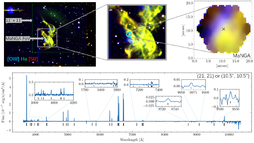
Figure 1: Upper: Criss-Cross Nebula (CCN) as seen at different scales. The left two images are constructed using narrowband images of [Sii] $\lambda\lambda$6717, 6731 and H$\alpha$ $\lambda$6563 from Temporin et al. (2007) and [Oiii] $\lambda\lambda$4959, 5007 obtained in this work. The rightmost image is based on MaNGA data of the same lines. Lower: the MaNGA spectrum of the central spaxel in the MaNGA field of view (marked as a black cross in the upper-right image). The short black lines below the spectrum indicate the position of 34 emission lines that are measured and studied in this work. Some of the lines are more closely shown in the insets.

A small part of the CCN has been observed as a filler target by the MaNGA survey, which is one of the three major experiments of the fourth generation Sloan Digital Sky Survey (SDSS-IV; Blanton et al., 2017). During its six-year operation from July 2014 through August 2020, MaNGA obtained integral-field spectroscopy (IFS) for $\gtrsim 10^{4}$ nearby galaxies selected from the NASA Sloan Atlas (NSA; Blanton et al., 2011). The IFS data were obtained using 17 science integral-field units (IFUs) with a field of view (FoV) ranging from $12^{\prime\prime}$ to $32^{\prime\prime}$ (Drory et al., 2015). The MaNGA spectra cover a wavelength coverage from 3600$\text{\AA}$ to 10300$\text{\AA}$ with a spectral resolution of $R\sim 2000$, taken with the two dual-channel BOSS spectrographs (Smee et al., 2013) on the Sloan 2.5-meter telescope at the Apache Point Observatory (Gunn et al., 2006). Details of MaNGA sample selection, flux calibration, survey execution and observing strategy can be found in Wake et al. (2017), Law et al. (2015), and Yan et al. (2016a, b). MaNGA raw data were reduced using the MaNGA data reduction pipeline (DRP; Law et al., 2016) which produces a 3D datacube for each target with an effective spatial resolution that can be described by a Gaussian with a full width at half maximum (FWHM) of $\sim 2.5^{\prime\prime}$. All the MaNGA data, including raw data and DRP products, are released as part of the final data release of SDSS-IV (DR17; Abdurro’uf et al., 2022).

We use the datacube produced by the MaNGA DRP for this study. The upper-right panel in Figure 1 shows the MaNGA FoV, a hexagon covering approximately $20^{\prime\prime}\times 20^{\prime\prime}$, thus only a small part of the CCN as indicated by the cyan hexagon in the upper-left and upper-middle panels. As an example, the lower panel of the same figure shows the spectrum of the central pixel (indicated by the black cross in the upper-right panel), with the short black lines marking some of the emission lines.

The MaNGA DRP creates a sky model for each plate based on data from the sky fibers, in a way that is designed and optimized for nearby galaxies. For the CCN, however, the “background” measured by the sky fibers is contaminated by the emission from diffuse ionized gas surrounding the CCN. We apply our spectral fitting method described in Section 2.3 to the sky model constructed by DRP, finding some emission lines to be over-subtracted. We do not attempt to rebuild the sky model. Rather, we measure the flux of these over-subtracted lines in the sky model, and we take into account their effect in the following analysis. A total of 4 emission lines are confirmed in the sky model including [Oii] $\lambda\lambda$3726, 3729 and [Sii] $\lambda\lambda$6717, 6731, whose redshifts are close to what we measured from the DRP datacube. We notice that the over-subtracted flux is typically one order of magnitude smaller than the flux measured from the DRP spectrum, and so the flux correction is generally a tiny effect on our results.

2.2 Ancillary data

We have obtained the [Oiii] $\lambda\lambda$4959, 5007 narrowband image for the whole CCN, using the China Near Earth Object Survey Telescope at Xuyi Observational Station operated by Purple Mountain Observatory (PMO). The observation was taken on December 30, 2021, with a total exposure time of 1.5 hours. In addition, kindly provided by Bringfried Stecklum, the narrowband images of [Sii] $\lambda\lambda$6717, 6731 and H$\alpha$ $\lambda$6563 used in T07 are also available for our study. The upper-left panel in Figure 1 shows the RGB image of the whole CCN, constructed by combining the narrowband images of [Oiii], H$\alpha$ and [Sii].

We observed the ¹²CO(1-0) line for the CCN using the PMO 13.7-m millimeter telescope (Zuo et al., 2004) located in Delingha, China, over the period from April 26, 2022 through May 6, 2022. A total of 136 scans were taken, and each scan was reduced to produce a datacube with a pixel size of 30^′′ by applying the standard reduction pipeline of this telescope. After fitting and subtracting the baseline in the spectrum and masking any heavily affected spectra, all unmasked spectra were stacked to create a final spectrum, which has a rms of $T_{\mathrm{CO}}=0.039\ \mathrm{K}$ in $0.15\ \mathrm{km/s}$. This spectrum provides no detection of ¹²CO(1-0) with a $3\sigma$ upper limit of $0.14\ \mathrm{K\ km/s}$ when assuming a line width of $10\ \mathrm{km/s}$. If we adopt a conversion factor of $\alpha_{\mathrm{CO}}=4.35\ (M_{\odot}/\mathrm{pc}^{2})/(\mathrm{K\ km/s})$, this upper limit corresponds to an H₂ surface density lower than $0.6\ M_{\odot}/\mathrm{pc}^{2}$.

2.3 Emission line measurements

The MaNGA spectra present numerous emission lines but almost no continuum over the whole wavelength coverage, as can be seen from the example spectrum in Figure 1. Therefore, for each spaxel we do not attempt to obtain an overall continuum component, and we directly apply our emission line fitting code to measure all the detected lines. These include a total of 34 emission lines, as listed in Table 1. Although the continuum is close to zero in all the spectra, the baseline beside each emission line always deviates to some degree from a zero horizontal line due to the residual in sky subtraction and/or flux calibration in the MaNGA DRP. We determine a local baseline with a linear fitting of the spectrum over both sides of each emission line, excluding obvious emission features and outliers by sigma clipping.

Each emission line is modeled with a single Gaussian. Most of the lines are well separated from each other, and each line is fitted independently. In some special cases as listed in Table 1, two or more neighboring lines are fitted simultaneously. In these cases some Gaussian function parameters may be tied for reasonable considerations, which are also listed and explained in the table. For a given line or a group of lines, the best-fit model is determined by minimizing the $\chi^{2}$, defined as

$$\chi^{2}=\sum_{i}^{n}\left(\frac{\mathrm{flux}_{i}-\mathrm{model}_{i}}{\mathrm{err}_{i}}\right)^{2},$$ (1)

where $n$ is the number of wavelength pixels over the emission line fitting window centered at the restframe wavelength of the line, $\mathrm{flux}_{i}$ and $\mathrm{model}_{i}$ are the observed and model fluxes of the $i$-th pixel, and $\mathrm{err}_{i}$ is the error of the observed flux of the $i$-th pixel. The width of the fitting window ranges from 20 $\text{\AA}$ to 100 $\text{\AA}$, mainly depending on the number of lines included in the fitting. As an example, Figure 2 displays the result of the fitting for all the 34 lines for the central spaxel in the MaNGA datacube. As can be seen, all the lines are well-fitted. In fact, the majority of the lines in the whole MaNGA datacube are well-fitted, except that for some weak lines such as [Ariii] $\lambda$7135, the emission line signal in some spaxels is overwhelmed by noise. In such cases, our fitting code gives best-fit models with small fluxes and relatively large uncertainties, which can be identified as non-detections given a signal-to-noise (S/N) threshold.

Table 1: All the lines fitted in MaNGA data

Line	3cmCenter wavelength	Model	Parameter tying	Notes	Morphological group
	$[\mathrm{\AA}]$
$\mathrm{[OII]}$ $\lambda$3726	3727.1	5cm$\sum_{i=1}^{i=2}$G${}_{i}(a_{i},\lambda_{i},\sigma_{i})$	5cm$\sigma_{1}=\sigma_{2}$		$\left\langle 3\right\rangle$
$\mathrm{[OII]}$ $\lambda$3729	3729.9				$\left\langle 3\right\rangle$
H$\eta$ $\lambda$3836	3836.5	G${}_{1}(a_{1},\lambda_{1},\sigma_{1})$			$\left\langle 2\right\rangle$
$\mathrm{[NeIII]}$ $\lambda$3869	3869.9	G${}_{1}(a_{1},\lambda_{1},\sigma_{1})$			$\left\langle 1\right\rangle$
H$\zeta$ $\lambda$3889	3890.2	G${}_{1}(a_{1},\lambda_{1},\sigma_{1})$			$\left\langle 2\right\rangle$
H$\epsilon$ $\lambda$3970	3971.2	G${}_{1}(a_{1},\lambda_{1},\sigma_{1})$			$\left\langle 2\right\rangle$
$\mathrm{[SII]}$ $\lambda$4069	4069.7	5cm$\sum_{i=1}^{i=3}$G${}_{i}(a_{i},\lambda_{i},\sigma_{i})$	6cm$\sigma_{1}=\sigma_{2}$		$\left\langle 2\right\rangle$
$\mathrm{[SII]}$ $\lambda$4076	4077.6				$\left\langle 2\right\rangle$
H$\delta$ $\lambda$4102	4102.9				$\left\langle 2\right\rangle$
H$\gamma$ $\lambda$4340	4341.7	G${}_{1}(a_{1},\lambda_{1},\sigma_{1})$			$\left\langle 2\right\rangle$
$\mathrm{[OIII]}$ $\lambda$4363	4364.4	G${}_{1}(a_{1},\lambda_{1},\sigma_{1})$			$\left\langle 1\right\rangle$
H$\beta$ $\lambda$4861	4862.8	G${}_{1}(a_{1},\lambda_{1},\sigma_{1})$			$\left\langle 2\right\rangle$
$\mathrm{[OIII]}$ $\lambda$4959	4960.3	G${}_{1}(a_{1},\lambda_{1},\sigma_{1})$			$\left\langle 1\right\rangle$
$\mathrm{[OIII]}$ $\lambda$5007	5008.3	G${}_{1}(a_{1},\lambda_{1},\sigma_{1})$			$\left\langle 1\right\rangle$
$\mathrm{[NI]}$ $\lambda$5200	5201.4	G${}_{1}(a_{1},\lambda_{1},\sigma_{1})$			$\left\langle 2\right\rangle$
$\mathrm{[NII]}$ $\lambda$5755	5756.2	G${}_{1}(a_{1},\lambda_{1},\sigma_{1})$			$\left\langle 2\right\rangle$
HeI $\lambda$5876	5877.2	G${}_{1}(a_{1},\lambda_{1},\sigma_{1})$			$\left\langle 2\right\rangle$
$\mathrm{[OI]}$ $\lambda$6300	6302.0	G${}_{1}(a_{1},\lambda_{1},\sigma_{1})$			$\left\langle 2\right\rangle$
$\mathrm{[OI]}$ $\lambda$6366	6368.1	G${}_{1}(a_{1},\lambda_{1},\sigma_{1})$			$\left\langle 2\right\rangle$
$\mathrm{[NII]}$ $\lambda$6548	6549.9	G${}_{1}(a_{1},\lambda_{1},\sigma_{1})$			$\left\langle 2\right\rangle$
H$\alpha$ $\lambda$6563	6564.6	G${}_{1}(a_{1},\lambda_{1},\sigma_{1})$			$\left\langle 2\right\rangle$
$\mathrm{[NII]}$ $\lambda$6583	6585.3	G${}_{1}(a_{1},\lambda_{1},\sigma_{1})$			$\left\langle 2\right\rangle$
$\mathrm{[SII]}$ $\lambda$6717	6718.3	G${}_{1}(a_{1},\lambda_{1},\sigma_{1})$			$\left\langle 2\right\rangle$
$\mathrm{[SII]}$ $\lambda$6731	6732.7	G${}_{1}(a_{1},\lambda_{1},\sigma_{1})$			$\left\langle 2\right\rangle$
$\mathrm{[ArIII]}$ $\lambda$7135	7137.8	G${}_{1}(a_{1},\lambda_{1},\sigma_{1})$			$\left\langle 1\right\rangle$
$\mathrm{[CaII]}$ $\lambda$7291	7293.5	8cm$\sum_{i=1}^{i=4}$G${}_{i}(a_{i},\lambda_{i},\sigma_{i})$			$\left\langle 2\right\rangle$
$\mathrm{[OII]}$ $\lambda$7320	7322.0		$\sigma_{1}=\sigma_{3}$		$\left\langle 1\right\rangle$
$\mathrm{[CaII]}$ $\lambda$7324	7325.9		$0.8<\sigma_{4}/\sigma_{2}<1.25$		$\left\langle 2\right\rangle$
$\mathrm{[OII]}$ $\lambda$7330	7332.0				$\left\langle 1\right\rangle$
$\mathrm{[CI]}$ $\lambda$8729	8729.5	G${}_{1}(a_{1},\lambda_{1},\sigma_{1})$			$\left\langle 2\right\rangle$
$\mathrm{[SIII]}$ $\lambda$9069	9071.4	G${}_{1}(a_{1},\lambda_{1},\sigma_{1})$			$\left\langle 1\right\rangle$
$\mathrm{[SIII]}$ $\lambda$9530	9534.7	G${}_{1}(a_{1},\lambda_{1},\sigma_{1})$			$\left\langle 1\right\rangle$
$\mathrm{[CI]}$ $\lambda$9826	9827.0	5cm$\sum_{i=1}^{i=2}$G${}_{i}(a_{i},\lambda_{i},\sigma_{i})$	5cm$\sigma_{1}=\sigma_{2}$		$\left\langle 2\right\rangle$
$\mathrm{[CI]}$ $\lambda$9852	9853.0				$\left\langle 2\right\rangle$

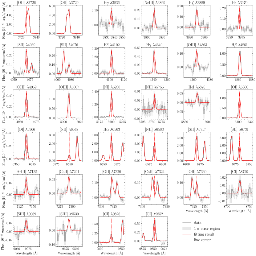
Figure 2: Fitting results for the 34 emission lines of one example spaxel. The grey histogram is the observed spectrum with baseline subtracted, and the shaded grey region is the 1 $\sigma$ error. The solid red line is the best-fit model, with the line center marked by the dashed vertical line.

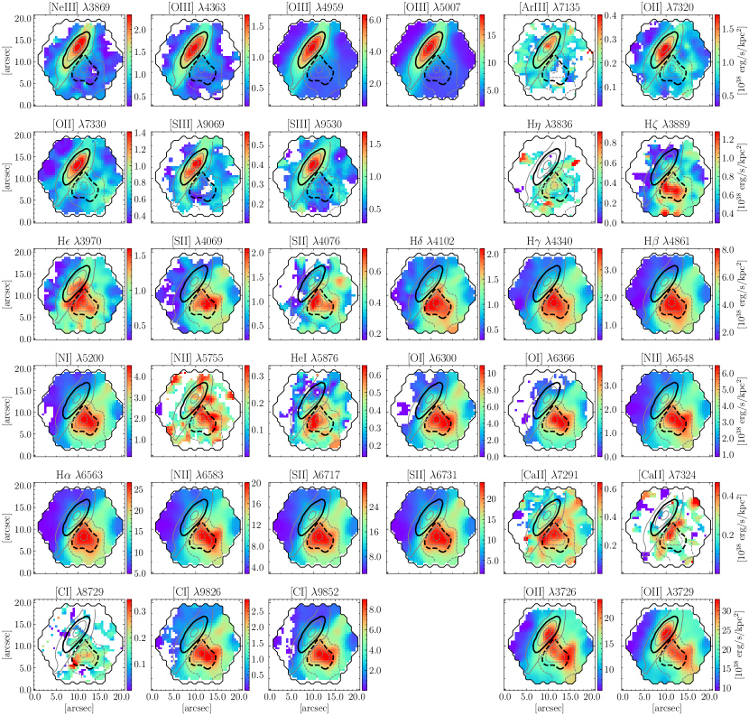
Figure 3: The surface brightness map of all the 34 emission lines measured within the MaNGA FoV in the unit of $10^{38}$ erg/s/kpc². The solid and dashed gray contours represent the 75%, 90% (bolded), 95%, and 99% quantiles in the surface brightness map of [Oiii] $\lambda$5007 and H$\alpha$ $\lambda$6563 lines, respectively, which are repeated in every panel for reference.

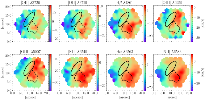
Figure 4: The velocity map of eight emission lines in the unit of km/s as measured from the MaNGA data. The bolded contours show 90% quantiles of [Oiii] $\lambda$5007 (solid line) and H$\alpha$ $\lambda$6563 (dashed line) surface brightness.

Figure 3 displays our measurements of the surface brightness map for all the 34 lines. In each panel we show the spaxels with S/N $>3$ only. According to the morphology of the maps, we find all the lines can be broadly divided into three groups. In the figure, the three groups of maps are shown separately with a blank gap inserted in between every two neighboring groups, while within each group the lines are ordered by increasing wavelength. As can be seen, the maps in the first group present a remarkable lane of high brightness across the upper-left part of the MaNGA FoV. This group consists of seven high-ionization lines and two [Oii] auroral lines: [Neiii] $\lambda$3869, [Oiii] $\lambda$4363, [Oiii] $\lambda$4959, [Oiii] $\lambda$5007, [Ariii] $\lambda$7135, [Oii] $\lambda$7320, [Oii] $\lambda$7330, [Siii] $\lambda$9069 and [Siii] $\lambda$9530. In what follows this group is referred to as “Group I”, or “[Oiii] $\lambda$5007-like group” to reflect the strongest fluxes of the [Oiii] $\lambda$5007 line in this group. We note that, for [Ariii] $\lambda$7135 the lane feature is less pronounced than other lines of the same group, but we still include it in Group I considering that the emission in the lane region is the strongest and the only significant feature of this line.

The second group is referred to as “Group II” or “H$\alpha$ $\lambda$6563-like group”, which is made up of 23 low-ionization or recombination lines: H$\eta$ $\lambda$3836, H$\zeta$ $\lambda$3889, H$\epsilon$ $\lambda$3970, [Sii] $\lambda$4069, [Sii] $\lambda$4076, H$\delta$ $\lambda$4102, H$\gamma$ $\lambda$4340, H$\beta$ $\lambda$4861, [Ni] $\lambda$5200, [Nii] $\lambda$5755, Hei $\lambda$5876, [Oi] $\lambda$6300, [Oi] $\lambda$6366, [Nii] $\lambda$6548, H$\alpha$ $\lambda$6563, [Nii] $\lambda$6583, [Sii] $\lambda$6717, [Sii] $\lambda$6731, [Caii] $\lambda$7291, [Caii] $\lambda$7324, [Oii] $\lambda$7330, [Ci] $\lambda$8729, [Ci] $\lambda$9826 and [Ci] $\lambda$9852. The main feature of this group is a clump-like emission region located in the lower-right part of the MaNGA FoV. Most of the maps in this group show a continuous area of clump, while some weak lines show more clumpy and less concentrated structures. We include both cases in this group, as long as the peak and the majority of the high brightness area are located in the lower-right part of the MaNGA FoV. The third group includes only two lines, [Oii] $\lambda$3726 and [Oii] $\lambda$3729, which show clump-like features at both the position of the [Oiii] $\lambda$5007 lane and the position of the H$\alpha$ clump, with a bridge-like structure connecting the two clumps.

To more clearly see the similarities of the maps within each group and the differences between different groups, in every panel we repeatedly show the brightness map of both [Oiii] $\lambda$5007 (the solid black contours) and H$\alpha$ $\lambda$6563 (the dashed contours). In the first group the lane-like feature shows up in all the maps with highly similar shapes and locations, while the clump-like feature seen in the H$\alpha$ map also similarly shows up in most of the maps in Group II. When comparing the two groups, it is noticeable that the lane-like feature in Group I has little spatial overlap with the clump-like feature in Group II. The spatial offset between the two groups of lines implies that the MaNGA region of the CCN is likely to be shocked by a blast wave moving from lower-right to upper-left. On the other hand, however, the fact that the H$\alpha$ bright region is clump-shaped instead of lane-shaped cannot be simply explained by a single shock.

Figure 4 displays the velocity map for eight emission lines which have reliable velocity measurements, typically with uncertainties less than $10\ \mathrm{km}/\mathrm{s}$. Overall, all the lines show relatively positive velocities in the lower-right region and negative velocities in the upper-left region. When comparing the velocity maps more closely, one can easily see both the high similarities within each group and the apparent differences between different groups. For instance, the velocity maps of [Oiii] $\lambda$5007 and [Oiii] $\lambda$4959 show a lane-like structure in the same position as their surface brightness maps, a unique feature which is not seen in the velocity maps of other groups. These velocity maps should in principle provide useful constraints to the physical processes behind the CCN. However, due to the limited spectral resolution of MaNGA, it is hard to decompose the different velocity components from the spectra. Therefore, we will use only the surface brightness measurements when constraining the shock models below in section 3.

3 Constraining shock models

3.1 The shock model

In this section, we attempt to fit the MaNGA data by applying the shock model implemented in the MAPPINGS V code (Sutherland & Dopita, 2017; Sutherland et al., 2018). The basic ideal of MAPPINGS V is to calculate the flow solution of one-dimensional radiative shock models with parallel-slab geometry. The cooling function is established based on the CHIANTI 8 atomic database (Del Zanna et al., 2015), and the pre-ionization effect is addressed via an iterative approach. Other than the usually used Rankine-Hugoniot flow equations, in MAPPINGS V a unique choosing of integral form of the conservation laws is employed to mitigate round-off errors. The reader is referred to Sutherland & Dopita (2017) for more details about MAPPINGS V.

To compare with the resolved MaNGA data, we use shock profiles calculated by the model, i.e. the physical properties and emissivity as functions of the separation $r$ from the shock front, instead of the integrated spectrum which is the default output of the model. In this case, the shock front locates at $r=0$, the region with $r>0$ has already been shocked (thus referred to as “shocked region”), and the region with $r<0$ is expected to be shocked in future (thus referred to as “precursor”). The precursor may have been ionized by the photons escaping from the shocked region. Since MAPPINGS V adopts parallel-slab geometry, in the direction perpendicular to the shock direction the physical properties and emissivity are homogenous in the model. Therefore, the model is essentially a one-dimensional model, and we need to simplify the geometry of the observed region in consideration in order for appropriate comparisons between model and data. Our geometry model is illustrated in Figure 5. We assume the region is a “slab” of ionized gas with a certain thickness, oriented with an inclination angle of $i$ (the angle between the “slab” and the line of sight). As a result, the gas slab has a line-of-sight depth of $D_{los}$, and so the slab thickness is given by $D=D_{los}\cos(i)$.

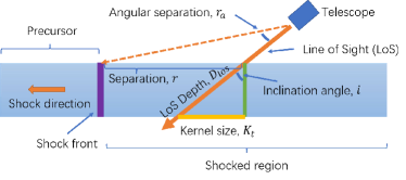
Figure 5: A sketch of the shock model adopted in our work. The shock is assumed to have a parallel-slab geometry with a depth of $D_{los}$ along the line of sight, and is orientated with an inclination angle of $i$. The vertical purple line marks the shock front, and the orange arrow in left side indicates the shock direction.

For a given emission line, the observed surface brightness profile, $F_{\mathrm{obs}}(r_{a})$ where $r_{a}$ is the angular separation from the shock front, can then be modelled by

$$F_{\mathrm{obs}}(r_{a})=G_{2.5}\star D_{los}[A(K_{t})\star f(r_{a})]+F_{b}.$$ (2)

In the equation, the symbol “$\star$” represents the convolution operation. Here, $f(r_{a})$ is the intrinsic emissivity profile given by the model. For the calculation of $f(r_{a})$, we adopt a distance of 150 pc to CCN in order to convert $r_{a}$ to physical separations with the consideration of projection effect (Uncertainties in CCN distance and the effects on our modelling will be discussed in subsection 4.1.). Due to the thickness and inclination of the gas region, the observed surface brightness at given $r_{a}$ is effectively an integral (along line of sight) of intrinsic emissivity at different physical separations. To take into account this effect, we first obtain an average surface brightness at $r_{a}$ by convolving $f(r_{a})$ with the averaging filter $A(K_{t})$ with a kernel size of $K_{t}=D_{los}\sin(i)$, which is then multiplied by the line-of-sight depth $D_{los}$ to give the total surface brightness, as can be seen from the first term at the right hand of Equation 2. This term is further convolved by $G_{2.5}$, a Gaussian filter with $\mathrm{FWHM}=2.5^{\prime\prime}$, which models the point spread function (PSF) of the MaNGA data. Finally, the last term of the equation represents an additional component, $F_{b}$, to account for the background emission which could be either a constant background/foreground in the line of sight (signal or noise, or both), or produced by ionizing mechanisms other than the shock. As we will show in subsection 3.2, the model with a constant background cannot explain our data. Thus, we have an extended model in subsection 3.3.

In addition, we also need to determine the location of the shock front and the projected direction of the shock. For simplicity, we fix the shock direction as the diagonal line going from the lower-right corner to the upper-left corner in the MaNGA FoV. This direction is perpendicular to the lane-like structure in the [OIII] surface brightness map, at which we have also seen sharp jumps in some line ratios (see Figure 6; the shock direction is indicated by the arrow in each panel). The shock should have moved from the H$\alpha$ clump region to the [Oiii] lane, so that the latter should be closer to the shock front. The location of the shock front cannot be determined by simple considerations, and this is modeled by a free parameter, $\Delta S$, the angular distance of the shock front to the central spaxel of the MaNGA FoV.

The physical parameters of the shock considered in this work include the pre-shock hydrogen density $n_{\mathrm{pre}}$, the shock velocity $v_{\mathrm{sh}}$, and the transverse magnetic field $B$. Considering the fact that CCN is projected in and also possibly located in the Orion-Eridanus superbubble, we adopt the metal abundance of the Orion nebula provided in MAPPINGS V. We note that changes in abundance can result in complex and non-linear modifications of shock properties. For instance, under certain parameters, a shock with a high metallicity can produce a higher [Oiii] $\lambda$5007/H$\beta$ $\lambda$4861 ratio when compared to its low metallicity counterpart. However, we find that, if the metallicity and abundance are not fixed, the model will have too many degrees of freedom and will be very hard to be constrained well with the available data. Therefore, we opt to fix the metallicity and abundance in this work and leave the effect of potential variations in metallicity or abundance to be studied in future when more data becomes available.

3.2 Model 1: shock with a constant background

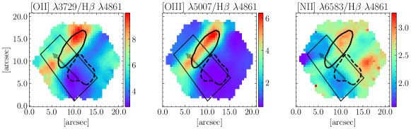
Figure 6: Maps of three line ratios: [Oii] $\lambda$3729/H$\beta$ $\lambda$4861, [Oiii] $\lambda$5007/H$\beta$ $\lambda$4861 and [Nii] $\lambda$6583/H$\beta$ $\lambda$4861. The “clean region” used to constrain the shock in Model 1 (see subsection 3.2) is indicated by a black quadrilateral. The gray arrow indicates the propagating direction of the shock. The bolded contours show 90% quantiles of [Oiii] $\lambda$5007 (solid line) and H$\alpha$ $\lambda$6563 (dashed line) surface brightness.

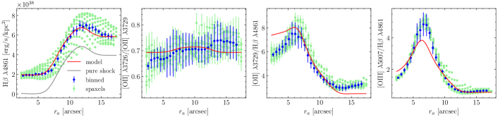
Figure 7: The shock profiles of H$\beta$ $\lambda$4861 surface brightness as well as emission lines ratios [Oii] 3726/3729, [Oii] $\lambda$3729/H$\beta$ $\lambda$4861 and [Oiii] $\lambda$5007/H$\beta$ 4861, as measured from the “clean region” in the MaNGA data and predicted by the best-fit Model 1. The green dots show the measurements for individual spaxels and the blue dots show the mean at given $r_{a}$ (angular distance from shock front). The solid red line is the best-fit model, while the grey line in the leftmost panel shows the model prediction without the constant background.

Table 2: The best-fit parameters of shock models with 1 $\sigma$ uncertainty

Model	$B$	$n_{\mathrm{pre}}$	$v_{\mathrm{sh}}$	$K_{t}$	$D_{los}$	$\Delta S$	$i=\arcsin(K_{t}/D_{los})$
	$[\mathrm{\mu G}]$	$[\mathrm{cm}^{-3}]$	$[\mathrm{km}/\mathrm{s}]$	$[\mathrm{AU}]$	$[\mathrm{AU}]$	$[\mathrm{arcsec}]$	$[\mathrm{deg}]$
Model 1 (H$\beta$)	$1.4\pm 1.2\times 10^{-4}$	$1.3\pm 0.2$	$112\pm 7$	$687\pm 65$	$1990\pm 453$	$7.2\pm 1.4$	$22\pm 7$
Model 1 (H$\alpha$)	$0.1\pm 0.1\times 10^{-5}$	$1.3\pm 0.2$	$110\pm 9$	$595\pm 60$	$1890\pm 415$	$7.4\pm 2.9$	$19\pm 5$
Model 2	$1.6\pm 0.3$	$1.4\pm 0.2$	$133\pm 5$	$419\pm 324$	$1150\pm 328$	$17.2\pm 3.8$	$19\pm 14$

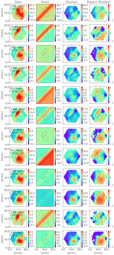
Figure 8: Surface density maps of 12 emission lines (panels from top to bottom). For each line, panels from left to right show the observed map, the predicted map by Model 1, and the absolute and relative residual maps. All the maps are color-coded by surface brightness in units of $10^{38}$ erg/s/kpc². The gray contours show 90% quantiles of [Oiii] $\lambda$5007 (solid line) and H$\alpha$ $\lambda$6563 (dashed line) surface brightness.

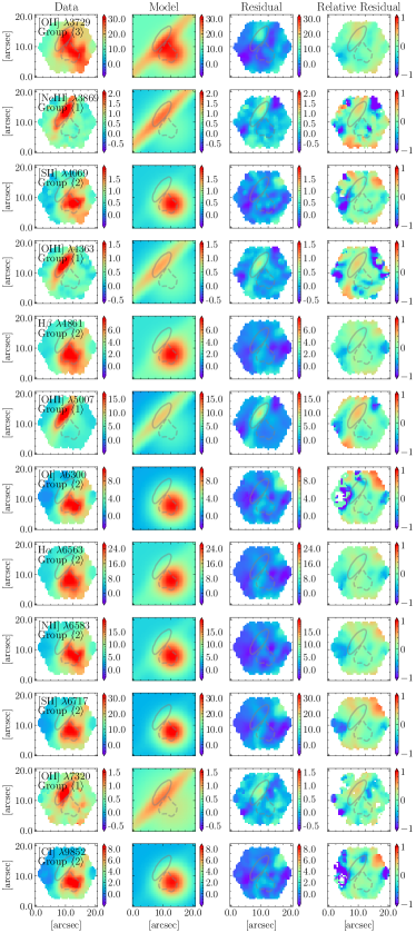
Figure 9: Same as Figure 8 but for Model 2.

We first consider the model with a constant background component. We have attempted to fit the shock and the background components simultaneously using all available line and line ratio measurements from the full MaNGA FoV, but finding ourselves unable to obtain a reasonably well constrained solution. We thus opt for a two-step approach, in which we first constrain the shock parameters, including both the physical parameters ($n_{\mathrm{pre}}$, $v_{\mathrm{sh}}$, $B$) and the geometric parameters ($K_{t}$, $D$, $\Delta S$), by applying the model to a selected set of emission lines and line ratios from a “clean region” selected out of the MaNGA FoV, and then we constrain the background component $F_{b}$ for all the emission lines from the full MaNGA FoV but fixing the parameters of the shock obtained from the first step.

The measurements used in the first step include the surface brightness profile of H$\beta$ $\lambda$4861 representing the H$\alpha$ $\lambda$6563-like group, the profile of [Oiii] $\lambda$5007 representing the [Oiii] $\lambda 5007$-like group, and the profiles of [Oii] $\lambda$3729 and [Oii] $\lambda$3726 from the third group. We include both lines from the [Oii] doublet because they are comparably strong, unlike the other two groups in which one or two lines are much stronger than the other lines. For the H$\alpha$ $\lambda$6563-like group, we use H$\beta$ rather than H$\alpha$ because the former is closer to [Oiii] $\lambda 5007$ in wavelength, and so the effect of dust extinction can be mitigated (although the dust extinction in CCN should be very weak; see subsection 4.2 for discussion). In fact, we have repeated the fitting procedure using H$\alpha$ to replace H$\beta$ in the first step, and we find very similar results (see Table 2).

The “clean region” used in the first step is indicated by a black quadrangle in each panel of Figure 6. This region is selected to have simple shock profiles in the line ratios along the projected direction of the shock (as indicated by the arrow). The exact boundary of this “clean region” is manually specified to maximize the number of spaxels included in the modelling, and at the same time to minimize the contamination of more complex features. We notice that the apparent difference between regions inside and outside the “clean region” is a hint that the whole region cannot be simply modeled with a single shock. We will come back and discuss this point in subsection 4.4.

It is time consuming to calculate the shock properties for a given set of model parameters, and so the calculation would be very expensive when the geometry parameters are fitted simultaneously with the shock parameters. In practice, we use a “zoom-in” grid fitting approach. We start with a coarse grid of the shock model parameters, and find the best-fit geometry parameters for each node of the grid by minimizing the reduced $\chi^{2}$. The best-fit model in this grid is then given by the node at which the reduced $\chi^{2}$ is the smallest over the whole grid, $\chi^{2}_{\mathrm{min}}$. A weight is then given to each of the nodes by $W=\mathrm{exp}(-\frac{1}{2}(\chi^{2}-\chi^{2}_{\mathrm{min}}))$, and the 1 $\sigma$ uncertainty of each parameter is calculated from the weighted average of all the nodes. If the uncertainties are significantly smaller than the step sizes of the grid, we construct a finer grid around the best-fit node and repeat the above process until the uncertainties are comparable with the step sizes of the grid.

The best-fit results from the first step are shown in Figure 7, where we plot the observed profiles from the clean region and the best-fit shock profiles. The best-fit model parameters and uncertainties are listed in Table 2. The model parameters constrained by using the H$\alpha$ line instead of H$\beta$ are also listed in the table. Generally, all the profiles are well-fitted in the whole range of $r_{a}$ probed, except that the model slightly overpredicts (underpredicts) the ratio of [Oii] $\lambda$3729/H$\beta$ $\lambda$4861 at the smallest (largest) $r_{a}$ (see the third panel of the figure) and the peak of [Oiii] $\lambda$5007/H$\beta$ $\lambda$4861 is a bit shallower in model. It is encouraging that the models with H$\beta$ and H$\alpha$ give rise to very similar constraints for all the model parameters. Accordingly, the shock has a velocity of $v_{\mathrm{sh}}\sim 110$ km/s, a pre-shock hydrogen density of $n_{\mathrm{pre}}\sim 1.3$ cm^-3, and a transverse magnetic field which is very close to zero (though with relatively large uncertainties). The shock velocity is larger than the value found by Z97, which is $40\ \mathrm{km}/\mathrm{s}$. This discrepancy may not be surprising, considering that the targeted position of the spectroscopic study in Z97 is outside the MaNGA FoV. The geometry parameters of our best-fit model show that the direction of shock is almost perpendicular to our line of sight, with an inclination angle of 22 deg (with H$\beta$) or 19 deg (with H$\alpha$). The shock front is about 7 arcsec from the central spaxel, thus close to the upper-left edge of the MaNGA FoV.

Figure 8 shows the best-fit results for some lines as obtained from the second step, in which we fix the shock model parameters and further constrain the background component for individual lines. For a given line, the figure displays the maps of the observed surface brightness, the surface brightness predicted by the model, the residual defined as the difference between the observation and model prediction ($\mathrm{Res}$), and the relative residual ($\mathrm{RR}$) defined as the ratio of the residual relative to the geometric mean of the surface brightness measurement and its error for each spaxel, i.e. $\mathrm{RR}=\mathrm{Res}/\sqrt{S^{2}+\mathrm{err}^{2}}$, where $S$ is the surface brightness of the emission line in the given spaxel, and $\mathrm{err}$ is the 1$\sigma$ uncertainty of the surface brightness. For spaxels with high S/N, the relative residual is effectively equal to fractional error, while for low S/N spaxels, the relative residual is reduced to the ratio between residual and measurement error, thus telling whether the residual can be explained by data uncertainties.

As can be seen, our model successfully captures some main features in the data, such as the [Oiii] lane-like structure and the overall difference in surface brightness between the upper-left and lower-right regions. However, the model substantially underpredicts or overpredicts the surface brightness for certain regions and for all the lines considered, which can be easily identified from the relative residual maps.

3.3 Model 2: shock with a 2D Gaussian component

The above result strongly suggests that the $F_{b}$ component in our model cannot be simply a constant background. We have considered a different model in which we add another shock, that is, the observed region is jointly ionized by two distinct shocks, but found such kind of model can not fit the data well (see subsection 4.5).

In this section we present our second model (Model 2 hereafter) in which we include a two-dimensional (2D) Gaussian component in addition to the shock component and the constant background. In this case, Equation 2 is rewritten as

$$F_{\mathrm{obs}}(x,y)=G_{2.5}\star D\{A(K_{t})\star f[r_{a}(x,y)]\}+F_{G}(x,y)+F_{b},$$ (3)

where the new term $F_{G}(x,y)$ is an isotropic 2D Gaussian function ($\sigma_{x}=\sigma_{y}$). Note that the observed surface brightness and the intrinsic emissivity are also written as two-dimensional functions of spaxel position $(x,y)$. This is because the total surface brightness in both data and model can no longer be described by a one-dimensional profile after the Gaussian component is included. Different emission lines share the same Gaussian center ($x,y$), but have their own width $\sigma_{x}$ and amplitude $A$. The fitting procedure is divided into two successive steps as for the first model (Model 1 hereafter). Different from Model 1, for the first step of Model 2 we use more emission lines and all available spaxels from the MaNGA FoV to constrain the shock parameters, considering the larger number of model parameters and the more complex model components. Specifically, we use the surface brightness profiles of [Oii] $\lambda$3729, H$\beta$ $\lambda$4861, [Oiii] $\lambda$5007, H$\alpha$ $\lambda$6563, [Nii] $\lambda$6583 and [Sii] $\lambda$6717.

This model can fit the data much better than Model 1, although the physical origin of the Gaussian component still remains unclear. The best-fit parameters and uncertainties of the shock component are listed in Table 2. Compared with Model 1, the shock in Model 2 has a slightly higher pre-shock hydrogen density (1.4 $\mathrm{cm}^{-3}$ versus 1.3 $\mathrm{cm}^{-3}$), slightly larger velocity (133 km/s versus $\sim$110 km/s), and a much stronger magnetic field (1.6 $\mu$G versus $\lesssim 10^{-4}$ $\mu$G). For the geometric parameters, both $K_{t}$ and $D$ are slightly smaller than those from Model 1, while $\Delta S$ increases from $\sim$7 arcsec to 17.2 arcsec. The inclination angles from the two models are quite similar, at around 19 deg.

The fitting results from the second step are shown in Figure 9, for the same set of emission lines as in the previous figure. As can be seen, the $\mathrm{RR}$ is significantly reduced in most spaxels and for all the lines when compared to the fitting results of Model 1. From the model-predicted maps, one can easily find both the differences between different groups of lines and the similarities within the same group: the three lines from the [Oiii] $\lambda 5007$-like group are uniformly dominated by the lane-like structure, the Gaussian component dominates all the lines from the H$\alpha$ $\lambda$6563-like group, and both components are presented in the map of [Oii] $\lambda 3729$ with comparable amplitudes. We have examined the ratios of different lines for the Gaussian component alone, finding them to be comparable to the expected line ratios of a clump of gas ionized by the photons from the shocked region (subsection 4.5). Although the fits are substantially improved with respect to Model 1, one can still see patterns of significant residuals. For instance, the maps tend to present positive values of $\mathrm{RR}$ in the left corner for the [Oiii] $\lambda$5007-like lines as well as the upper-right edge for the H$\alpha$ $\lambda$6563-like lines. At the border of the MaNGA FoV, these regions could be adjacent to other regions of the CCN that may be ionized in a different way. In addition, a lane-like residual pattern can be seen in/around the original [Oiii] lane structure, for all the emission lines but with different orientations for different line groups. This pattern is likely to be induced by another shock along the upper-right to lower-left direction. We will come back and discuss on this point in subsection 4.4.

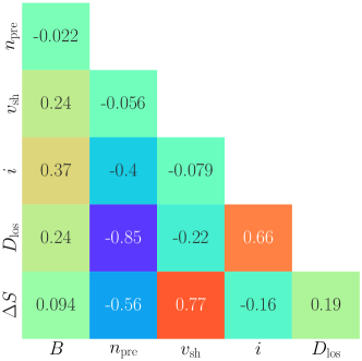
Figure 10: The weighted Pearson correlation coefficients for best-fit parameters of Model 2.

We evaluate the correlations between model parameters by calculating the weighted Pearson correlation coefficient $r_{\mathrm{pearson}}$ based on the grid generated during the fitting process. The result is shown in Figure 10 for the six free parameters describing the shock and the geometry. The shock parameters ($v_{\mathrm{sh}}$, $n_{\mathrm{pre}}$, $B$) show weak correlations between each other, but they all show strong correlations with one or more geometric parameters. This analysis suggests that, though not very strong, our model suffers from degeneracies caused by the projection effect and the uncertainties in the geometry of the gas region. We would like to point out that the degeneracies between model parameters are taken into account in the 1$\sigma$ uncertainties of our best-fit model parameters, which are actually the weighted standard deviation of the marginalized distributions.

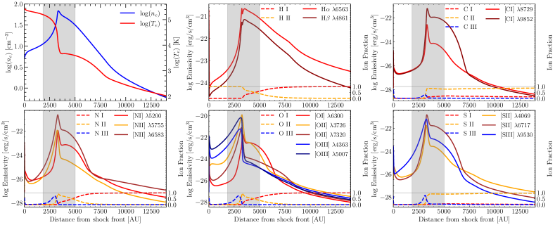
Figure 11: In the top left panel, we present the intrinsic shock profiles of the electronic density ($n_{e}$) in blue and the temperature ($T_{e}$) in red, as predicted by Model 2. The remaining panels display the ion fractions of hydrogen (H), carbon (C), nitrogen (N), oxygen (O), and sulfur (S), as well as the emissivity of the corresponding emission lines. These panels are arranged from left to right and top to bottom. The shaded region in each panel represents the coverage of the MaNGA FoV.

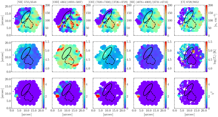
Figure 12: The electron density map (first row) and temperature map (second row) as measured from the combinations of density-sensitive line ratio [Sii] 6731/6717 and different temperature-sensitive line ratios (panels from left to right): [Nii] 5755/6548, [Oiii] 4363/(4959+5007), [Oii] (7320+7330)/(3726+3729), [Sii] (4076+4069)/(6731+6716), and [Ci] 8729/9852. The bottom panels show the corresponding $\chi^{2}$ maps. The bolded contours in each panel show 90% quantiles of [Oiii] $\lambda$5007 (solid line) and H$\alpha$ $\lambda$6563 (dashed line) surface brightness.

3.4 Shock profiles of electron temperature and density

The top-left panel of Figure 11 displays the profiles of both electron temperature $T_{e}$ (the red curve) and density $n_{e}$ (the blue curve) in the shock component as predicted by our best-fit model (Model 2). Plotted in the other panels are the emissivity profiles (solid lines) and the corresponding ion fraction profiles (dashed lines) of hydrogen (H), carbon (C), nitrogen (N), oxygen (O) and sulfur (S). As can be seen, the MaNGA FoV (indicated by the gray band) happens to capture the jump in density and temperature (and subsequently, the line emissivities) at $r\sim 3500$ AU.

An alternative and more commonly-adopted way to measure temperatures and densities of ionized gas is to use a set of selected emission line ratios that are sensitive to $n_{e}$ or $T_{e}$ as diagnostics, based on a given atomic database. It is interesting to compare the $T_{e}$ and $n_{e}$ profiles predicted by our model with those calculated directly from emission line ratios. We use PyNeb (Luridiana et al., 2015) to calculate $T_{e}$ and $n_{e}$ for each spaxel within the MaNGA FoV based on our measurements of emission line ratios. For consistency, we use CHIANTI 8 (Del Zanna et al., 2015), the same atomic database as used in MAPPINGS V. In fact, we have explored alternative databases available in PyNeb, finding them to provide similar $n_{e}$ and $T_{e}$. We use the line ratio of [Sii] 6731/6717 as the diagnostic of $n_{e}$, and use five different line ratios as diagnostics of $T_{e}$: [Nii] 5755/6548, [Oiii] 4363/(4959+5007), [Oii] (7320+7330)/(3726+3729), [Sii] (4076+4069)/(6731+6716), and [Ci] 8729/9852. For a given pair of $T_{e}$-sensitive and $n_{e}$-sensitive diagnostics, we obtain the measurements of $T_{e}$ and $n_{e}$ simultaneously for each spaxel in the MaNGA FoV. Therefore, five combinations of $T_{e}$-sensitive line ratios and the $n_{e}$-sensitive line ratio give rise to a set of five measurements of the $T_{e}$ and $n_{e}$ maps, which are shown in the top and middle rows in Figure 12.

Each combination utilizes different $T_{e}$-sensitive line ratios while keeping the $n_{e}$-sensitive line ratio fixed as [Sii] 6731/6717. The alternative $n_{e}$-sensitive line ratio [Oii] 3726/3729 is not utilized due to its significant uncertainty, as illustrated in the second panel of Figure 7. This uncertainty obscures the true density structure and generates a misleading clumpy artificial density distribution. The primary cause of this significant uncertainty stems from that the [Oii] $\lambda\lambda$ 3726,3729 doublets is not well resolved in the MaNGA spectra, as can be seen in the first two panels of Figure 2. Therefore, using [Oii] 3726/3729 would risk over-interpreting the data. However, it would be worthwhile to investigate the consistency between the density measured by [Oii] 3726/3729 and [Sii] 6731/6717 when higher quality data becomes available. It is important to note that, although $n_{e}$ is mainly constrained by [Sii] 6731/6717, the different $T_{e}$-sensitive lines lead to slight differences in the derived $n_{e}$. This is why the $n_{e}$ maps in the first row of Figure 12 differ quantitatively, although they qualitatively show good agreement. The bottom row in the same figure shows the corresponding $\chi^{2}$ maps. As can be seen, the $\chi^{2}$ values are close to zero in most spaxels of a given map, indicating that all the lines relevant for measuring $T_{e}$ and $n_{e}$ are well-fitted. We note that, we have added back the over-subtracted sky flux when calculating [SII] $\lambda\lambda$ 6717,6731, although this correction has no significant effect on our results.

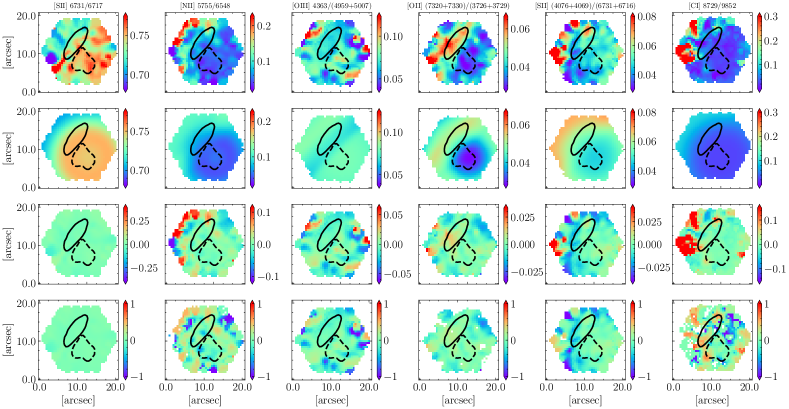
Figure 13: Shown in the top panels are the observed surface density maps of six emission line ratios that are used to measure electronic density and temperature maps in the previous figure (Figure 12). The predicted maps of the same lines by Model 2 are shown in the panels in the second row. The third and last rows show the absolute and relative residual maps.

From Figure 12, all the density maps present a prominent jump from the upper-left low density region ($\sim 1\ \mathrm{cm}^{-3}$) to the lower-right high density region ($\sim 100\ \mathrm{cm}^{-3}$), and the boundary of the two regions coincides with the location of the lane-like structure in the surface brightness maps of the [Oiii] $\lambda 5007$-like group. This result qualitatively agrees with the predicted density profile in Figure 11. Unlike $n_{e}$, the measurements of $T_{e}$ are different, depending on what temperature diagnostics are used. In this case, only [Oii] (7320+7330)/(3726+3729) captures the overall trend of the predicted temperature profile in Figure 11. However, we should note that it is not suitable to directly compare the profiles shown in Figure 11 with the measurements in Figure 12, as the former are the intrinsic shock profiles without the Gaussian component and observational effects (e.g. limited spatial resolution and projection effect) in the real data.

In Figure 13 we compare the observed maps of the diagnosing line ratios (panels in the top row) with the predicted maps of the same line ratios from Model 2 in which we have included both the Gaussian component and the observational effects. Overall, our model can well reproduce the distribution of all the line ratios (the second row), although with subtle structures remaining in the maps of absolute residual (the third row) and relative residual (the bottom row). This result demonstrates that the discrepancies in $T_{e}$ as measured from different line ratios are caused by observational effects as well as the contamination of non-shock components such as the Gaussian component in our case. It appears that different line ratios can be affected by these effects in different ways, thus leading to inconsistent measurements. We have examined the effect of the Gaussian component and the observational effects separately, and we find both effects to have contributed significantly to the total discrepancies. Our analysis thus strongly warns that electronic density and temperature measurements based on observed emission line ratios can be seriously biased due to observational effects and non-shock components, and should be taken with caution.

4 Discussion

4.1 The distance to CCN

If assumed to be a part of the Orion-Eridanus superbubble, CCN should be at a distance ranging from $150\ \mathrm{pc}$ to $400\ \mathrm{pc}$, corresponding to the close and far ends of the superbubble (Pon et al., 2016; Kounkel et al., 2017; Zari et al., 2017). Using the three-dimensional extinction map constructed by Vergely et al. (2022), we find the differential extinction along the line of sight to CCN to present two peaks, located at $150\ \mathrm{pc}$ and $475\ \mathrm{pc}$, respectively. The two peaks coincide with the two edges of the Orion-Eridanus superbubble, and the CCN is likely to be associated with one of the peaks. In addition, we have attempted to constrain the distance to CCN with our data, by including the distance as a free parameter in Model 2, $D_{\mathrm{CCN}}$. We obtain a best-fit distance of $D_{\mathrm{CCN}}=170\pm 94\ \mathrm{pc}$. This value is still consistent with the values from the first two considerations, given the large uncertainties. This result implies that the distance cannot be well constrained given the currently available data. Fortunately, we found that both the $B$ and $v_{\mathrm{sh}}$ have a weak correlation with the distance of CCN. On the other hand, although $n_{\mathrm{pre}}$ has a stronger correlation with $D_{\mathrm{CCN}}$, the marginalized uncertainty of $n_{\mathrm{pre}}$ only increases from $1.4\pm 0.2\ \mathrm{cm}^{-3}$ to $1.4\pm 0.3\ \mathrm{cm}^{-3}$. The geometry parameters are indeed correlated with the distance, but our test shows that the data still prefer a small inclination angle, with models of $i<30\ \mathrm{deg}$ showing a larger Bayesian evidence than those of $i\geq 30\ \mathrm{deg}$.

4.2 The dust extinction in CCN

The dust extinction in CCN is also uncertain. An upper limit of the dust extinction along the line of sight towards CCN can be estimated by integrating the differential extinction from Vergely et al. (2022) over the distance range from 0 up to 475 $\mathrm{pc}$. This gives rise to $A_{5500\text{\AA}}$ = 0.14 $\mathrm{mag}$, corresponding to a color excess of $\mathrm{E}(\mathrm{B}-\mathrm{V})<0.05$ mag assuming the Milky Way extinction curve of Cardelli et al. (1989) with $\mathrm{R}_{\mathrm{V}}=3.1$. This is smaller than the average value estimated from H$\alpha$ $\lambda$6563/H$\beta$ $\lambda$4861 in the MaNGA FoV, $\mathrm{E}(\mathrm{B}-\mathrm{V})=0.12$ mag, using the electronic temperature for each spaxel as constrained by our best-fit model and assuming the Case B recombination coefficient. We find that, however, different Balmer line ratios lead to inconsistent $\mathrm{E}(\mathrm{B}-\mathrm{V})$ values, implying that the extinction curve of Cardelli et al. (1989) may not be applicable for CCN, or that the Case B assumption is not appropriate in shocked regions (e.g. see Figure 4 of Dopita & Sutherland 2017). In fact, our best-fit shock model does predict higher H$\alpha$ $\lambda$6563/H$\beta$ $\lambda$4861 ratios than that of Case B at fixed temperature. We have also attempted to include the dust extinction in our model. We find no significant improvement in goodness-of-fit, and the null hypothesis of ${E}(\mathrm{B}-\mathrm{V})=0$ can not be rejected at a 3$\sigma$ level. In summary, though without direct measurements of the dust content, constraints from different aspects consistently suggest that the dust extinction in CCN is rather limited. Our modelling presented in the previous section should have not been affected significantly by dust extinction.

4.3 A single shock interacting with a cold gas cloud, or multiple shocks?

The MaNGA data and our best-fit model suggest that the CCN region observed by MaNGA is ionized by a shock which moves across the MaNGA FoV from the lower-right corner to the upper-left corner. This direction is opposite to the shock direction indicated by the protruding double-arc structure of the whole CCN, which goes from left to right as suggested by Z97 and T07. A natural explanation on this discrepancy is that CCN is a shocked cloud of cold gas (atomic gas, or molecular gas, or both). In this case, the overall curvature in the emission line surface brightness maps traces the shape of the gas cloud, but not the shock front. The protruding arcs to the right are actually the right edge of the cloud, which has collided head-on with the shock wave coming from the right. The shock has already swept into but not through the cloud, and consequently the shock front is found on the left side of the arc and still within the cloud. In a recent theoretical study by Kupilas et al. (2022), the simulation of a shocked Hi cloud produces a double-arc structure which is similar to CCN (see their Figure 4). Accordingly, one would expect to detect Hi on the left side of the double arc. We have examined the Hi data of the Galactic All Sky Survey (GASS; McClure-Griffiths et al., 2009; Kalberla et al., 2010), finding no Hi enhancement at the position of CCN. Considering the low spatial resolution of GASS ($14.4^{\prime}$), however, the Hi cloud may suffer from smearing effect and so the scenario of a shocked Hi cloud cannot be firmly ruled out with the current data. As abovementioned, we have also used the Purple Mountain Observatory (PMO) 13.7-m millimeter telescope to observe the ¹²CO(1-0) line in CCN (subsection 2.2). This observation provides an upper limit of the H₂ surface density, which is $0.6\ M_{\odot}/\mathrm{pc}^{2}$ if we assume a conversion factor of $\alpha_{\mathrm{CO}}=4.35\ (M_{\odot}/\mathrm{pc}^{2})/(\mathrm{K\ km/s})$ and a line width of $10\ \mathrm{km/s}$. This result largely rules out the scenario of a shocked molecular cloud, consistent with the simulation in Kupilas et al. (2022) where the CCN-like double arc can not be formed in a shocked H₂ cloud (see their Figure 9).

The double-arc structure of the CCN could also be produced by multiple shocks, rather than the interaction between a cold gas cloud and a single shock as discussed above. In fact, the idea of multiple shocks has its own supporting evidences, including significant differences in the line ratio distributions in/outside the “clean region” in Figure 6, residuals of the best-fit model in Figure 9, the double-arc structure of the whole CCN, and the variation of shock velocity in different regions of CCN (e.g. $133\ \mathrm{km/s}$ in the MaNGA FoV studied in our work versus $40\ \mathrm{km/s}$ in the region studied by Z97). It’s likely that there are two or even more shocks with different orientations in the CCN region.

Both IFU observations covering the whole CCN and high-resolution Hi observations would be needed if one were to discriminate the scenario of gas cloud with a single shock and the picture of multiple shocks.

4.4 Source of the shock

No matter which scenario is at work, as Z97 and T07 suggested, the source of the shock is most likely to be a supernova, which may be the one responsible for the Orion-Eridanus superbubble. In this case, however, the shock direction should go from left to right, thus in disfavor of the Hi cloud scenario. In addition, we failed to find any candidates of source supernova after having searched known supernovae and pulsars around CCN. Thus, the source of CCN is still an open question.

4.5 The Gaussian component

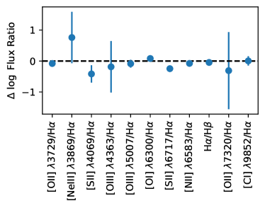
Figure 14: The residual of the best-fit integrated shock model obtained by comparing it with the line ratio of the Gaussian component. The error bar represents the 1 $\sigma$ uncertainty of the line ratio of the Gaussian component.

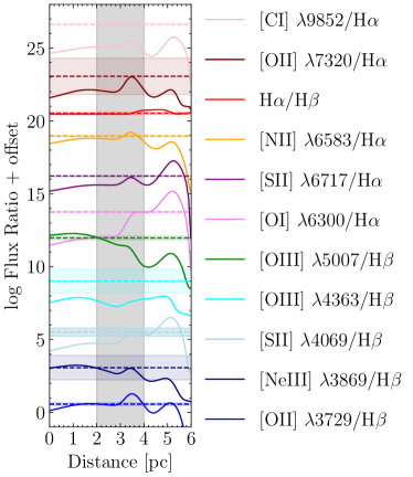
Figure 15: The line ratio profile of the precursor of Model 2 (solid line) is compared to the fitted line ratio of the Gaussian component (represented by the horizontal dashed line). The colorful shaded region represents the 1 $\sigma$ uncertainty of the fitted line ratio of the Gaussian component. Additionally, the grey shaded region indicates the coverage of the MaNGA FoV.

The physical origin of the Gaussian component is not immediately clear from our results. This component is possibly caused by another resolved shock. We have attempted to fit the residual of the shock component in Model 2 with another shock moving in the same direction, i.e. from lower-right to upper-left in the MaNGA FoV. We find that, however, some emission lines such as [Sii] $\lambda$6717 and [Nii] $\lambda$6583 cannot be fitted by this model. We have also tried with a shock direction from upper-right to lower-left, which fails to fit the lines in Group II. Another possible case is that the second shock propagates along the line of sight. We thus use an integrated shock model (the default output of the MAPPINGS V) to fit the line ratios in the Gaussian component. We find that a shock with $n_{\mathrm{pre}}=0.1\ \mathrm{cm}^{-3}$, $v_{\mathrm{sh}}=450\ \mathrm{km}/\mathrm{s}$, and $B=0.1\ \mathrm{\mu G}$ can explain all the line ratios except [Sii]$\lambda$6717/H$\alpha$ and [Sii]$\lambda$4069/H$\alpha$, as can be seen from Figure 14. Given the high velocity of this shock, we would expect the velocity field at the location of the Gaussian component to differ significantly from the other regions. However, this is not observed in the MaNGA FoV (see Figure 4). Therefore, another shock is unlikely to be the origin of the Gaussian component.

Alternatively, the Gaussian component could be a clump of gas near the shocked region. In this scenario, the gas in this clump can be ionized by photons from shocked region. The most likely candidate that can be modeled with MAPPINGS V is the precursor of the shock in Model 2. Although this gas clump may have a different geometry than the precursor, most of the line ratios of the Gaussian component agree with the line ratio profiles of the shock precursor as predicted by Model 2 with a precusor-to-shock front distance of 2-4 pc, as shown in Figure 15. Two of the line ratios, [Ci] $\lambda$9852/H$\alpha$ $\lambda$6563 and [Oiii] 4363/H$\beta$ $\lambda$4861 show discrepancies between the data and the model, which could be attributed to a variety of reasons, e.g. the homogenous gas assumption adopted in MAPPINGS V, differences in the geometry of this gas clump compared to the precursor component in MAPPINGS V, differences in the metal abundance of the gas compared to our assumptions, or the contribution of photons from the shocked region outside the MaNGA FoV. However, investigation of these possibilities is beyond the scope of the current paper. Considering that the majority of the line ratios can be explained with no additional free parameters, we suggest that the Gaussian component is very likely a clump of gas ionized by photons from the shocked region, thus physically related to the shocked region. Further studies in future are needed to pin down this scenario.

5 Summary

In this work, we have analyzed the integral field spectroscopy data for a small part of the Criss Cross Nebula (CCN), which was observed as a filler target by the MaNGA survey (Figure 1). At a distance of $\sim 150-475$ pc, the spatial resolution of MaNGA ($\sim 2.5^{\prime\prime}$) corresponds to a physical scale less than 1000 AU. Within the MaNGA FoV, a hexagon covering $\sim 20^{\prime\prime}\times 20^{\prime\prime}$, we have obtained the surface brightness map for 34 emission lines in the optical band, by fitting Gaussian profiles to the observed spectrum of each spaxel (Table 1 and Figure 2). We find the emission lines can be broadly divided into three groups according to their surface brightness maps (Figure 3): (1) the [Oiii] $\lambda$5007-like group including seven high-ionization lines and two [Oii] auroral lines which uniformly present a remarkable lane of high brightness in the upper-left part of the MaNGA FoV, (2) the H$\alpha$ $\lambda$6563-like group including 23 low-ionization or recombination lines which mostly present a clump of high brightness in the lower-right part of the MaNGA FoV, and (3) the third group including only two lines, [Oii] $\lambda$3726 and [Oii] $\lambda$3729, which show clump-like structures at positions of both the [Oiii] $\lambda$5007 lane and the H$\alpha$ $\lambda$6563 clump. The velocity maps of different lines in a given group show high similarities, but vary from group to group (Figure 4). The three categories of microstructures indicate both regularity and complexity in the CCN.

We assume the lane structure in the [Oiii] $\lambda$5007-like group is produced by a shock which is moving across the CCN from the lower-right to upper-left direction. We use the measurements of emission line brightness and surface brightness ratios between different lines to constrain both physical parameters and geometry parameters of the shock model. We have examined two models: a simple model with a single shock plus a constant background (Model 1; Equation 2), and a more complex model with an additional Gaussian component (Model 2; Equation 3). We show that the MaNGA data can be reasonably well-fitted with Model 2 (Figure 8; Figure 9). The physical counterpart of the Gaussian component is likely another clump of gas ionized by photons from the shocked region (Figure 15), though more data is needed to further confirm this scenario. Our best-fit model parameters indicate that the shock has a pre-shock hydrogen density of $n_{\mathrm{pre}}=1.4\pm 0.2$ cm^-3, a velocity of $133\pm 5$ km/s, and a transverse magnetic field of $B=1.6\pm 0.3$ $\mu$G, with the shock direction orientated to the line of sight by an inclination angle of $19\pm 14$ deg (Table 2; Figure 5).

Finally, we have compared the electronic density and temperature profiles as predicted by Model 2 (Figure 11) with those calculated directly using observed emission line ratios as commonly-done in the literature (Figure 12). We find different line ratios to give rise to similar density maps but significantly inconsistent temperature maps. The discrepancies can be attributed to observational effects caused by the limited spatial resolution of the data and the projection of the shock geometry, as well as the contamination of the additional Gaussian component. After including all these effects, our model can well reproduce all the emission line ratios that are relevant for calculating density and temperature (Figure 13). Thus, electronic densities and temperatures measured from observed line ratios should be taken with caution (see also Cameron et al. 2022 for a similar caveat).

The CCN is an ideal lab for studying microstructures in shock regions and testing existing shock models. Considering its nearby distance, relatively high surface brightness and unique morphology, CCN will be a good template for studying similar nebulae in greater distance, e.g. those being/to be observed by the Local Volume Mapper of the SDSS V project (Konidaris et al., 2020) and the AMAZE project (Yan et al., 2020). For the CCN itself, as mentioned, future studies would benefit from high-resolution Hi and IFS observations, both covering the whole CCN. In fact, we have recently done both observations, using MeerKAT and SITELLE on CFHT, and we expect to come back and present more scientific results soon.

References

- Abdurro’uf et al. (2022) Abdurro’uf, Accetta, K., Aerts, C., et al. 2022, ApJS, 259, 35, doi: 10.3847/1538-4365/ac4414
- Alarie & Drissen (2019) Alarie, A., & Drissen, L. 2019, MNRAS, 489, 3042, doi: 10.1093/mnras/stz2279
- Alatalo et al. (2016) Alatalo, K., Cales, S. L., Rich, J. A., et al. 2016, ApJS, 224, 38, doi: 10.3847/0067-0049/224/2/38
- Astropy Collaboration et al. (2013) Astropy Collaboration, Robitaille, T. P., Tollerud, E. J., et al. 2013, A&A, 558, A33, doi: 10.1051/0004-6361/201322068
- Astropy Collaboration et al. (2018) Astropy Collaboration, Price-Whelan, A. M., Sipőcz, B. M., et al. 2018, AJ, 156, 123, doi: 10.3847/1538-3881/aabc4f
- Astropy Collaboration et al. (2022) Astropy Collaboration, Price-Whelan, A. M., Lim, P. L., et al. 2022, apj, 935, 167, doi: 10.3847/1538-4357/ac7c74
- Blanton et al. (2011) Blanton, M. R., Kazin, E., Muna, D., Weaver, B. A., & Price-Whelan, A. 2011, AJ, 142, 31, doi: 10.1088/0004-6256/142/1/31
- Blanton et al. (2017) Blanton, M. R., Bershady, M. A., Abolfathi, B., et al. 2017, AJ, 154, 28, doi: 10.3847/1538-3881/aa7567
- Bundy et al. (2015) Bundy, K., Bershady, M. A., Law, D. R., et al. 2015, ApJ, 798, 7, doi: 10.1088/0004-637X/798/1/7
- Cameron et al. (2022) Cameron, A. J., Katz, H., & Rey, M. P. 2022, arXiv e-prints, arXiv:2210.14234. https://arxiv.org/abs/2210.14234
- Cardelli et al. (1989) Cardelli, J. A., Clayton, G. C., & Mathis, J. S. 1989, ApJ, 345, 245, doi: 10.1086/167900
- Carpenter et al. (1995) Carpenter, J. M., Snell, R. L., & Schloerb, F. P. 1995, ApJ, 445, 246, doi: 10.1086/175692
- Chevalier (1999) Chevalier, R. A. 1999, ApJ, 511, 798, doi: 10.1086/306710
- Chevalier & Gull (1975) Chevalier, R. A., & Gull, T. R. 1975, ApJ, 200, 399, doi: 10.1086/153802
- Clark & Stephenson (1977) Clark, D. H., & Stephenson, F. R. 1977, The historical supernovae
- da Costa-Luis (2019) da Costa-Luis, C. O. 2019, Journal of Open Source Software, 4, 1277
- Davidson & Fesen (1985) Davidson, K., & Fesen, R. A. 1985, ARA&A, 23, 119, doi: 10.1146/annurev.aa.23.090185.001003
- Del Zanna et al. (2015) Del Zanna, G., Dere, K. P., Young, P. R., Landi, E., & Mason, H. E. 2015, A&A, 582, A56, doi: 10.1051/0004-6361/201526827
- Deng et al. (2022) Deng, Y., Zhang, Z.-Y., Zhou, P., et al. 2022, arXiv e-prints, arXiv:2210.16909. https://arxiv.org/abs/2210.16909
- Dopita et al. (1997) Dopita, M. A., Koratkar, A. P., Allen, M. G., et al. 1997, ApJ, 490, 202, doi: 10.1086/304862
- Dopita & Sutherland (2017) Dopita, M. A., & Sutherland, R. S. 2017, ApJS, 229, 35, doi: 10.3847/1538-4365/aa6542
- Dopita et al. (2015) Dopita, M. A., Ho, I. T., Dressel, L. L., et al. 2015, ApJ, 801, 42, doi: 10.1088/0004-637X/801/1/42
- Drory et al. (2015) Drory, N., MacDonald, N., Bershady, M. A., et al. 2015, AJ, 149, 77, doi: 10.1088/0004-6256/149/2/77
- Farage et al. (2010) Farage, C. L., McGregor, P. J., Dopita, M. A., & Bicknell, G. V. 2010, ApJ, 724, 267, doi: 10.1088/0004-637X/724/1/267
- Fesen et al. (1997) Fesen, R. A., Shull, J. M., & Hurford, A. P. 1997, AJ, 113, 354, doi: 10.1086/118258
- Gunn et al. (2006) Gunn, J. E., Siegmund, W. A., Mannery, E. J., et al. 2006, AJ, 131, 2332, doi: 10.1086/500975
- Harris et al. (2020) Harris, C. R., Millman, K. J., van der Walt, S. J., et al. 2020, Nature, 585, 357, doi: 10.1038/s41586-020-2649-2
- Hester (2008) Hester, J. J. 2008, ARA&A, 46, 127, doi: 10.1146/annurev.astro.45.051806.110608
- Ho et al. (2014) Ho, I. T., Kewley, L. J., Dopita, M. A., et al. 2014, MNRAS, 444, 3894, doi: 10.1093/mnras/stu1653
- Holden et al. (2023) Holden, L. R., Tadhunter, C. N., Morganti, R., & Oosterloo, T. 2023, MNRAS, 520, 1848, doi: 10.1093/mnras/stad123
- Hunter (2007) Hunter, J. D. 2007, Computing in Science & Engineering, 9, 90, doi: 10.1109/MCSE.2007.55
- Jones et al. (1998) Jones, T. W., Rudnick, L., Jun, B.-I., et al. 1998, PASP, 110, 125, doi: 10.1086/316122
- Kalberla et al. (2010) Kalberla, P. M. W., McClure-Griffiths, N. M., Pisano, D. J., et al. 2010, A&A, 521, A17, doi: 10.1051/0004-6361/200913979
- Konidaris et al. (2020) Konidaris, N. P., Drory, N., Froning, C. S., et al. 2020, in Society of Photo-Optical Instrumentation Engineers (SPIE) Conference Series, Vol. 11447, Ground-based and Airborne Instrumentation for Astronomy VIII, ed. C. J. Evans, J. J. Bryant, & K. Motohara, 1144718, doi: 10.1117/12.2557565
- Kounkel et al. (2017) Kounkel, M., Hartmann, L., Loinard, L., et al. 2017, ApJ, 834, 142, doi: 10.3847/1538-4357/834/2/142
- Kupilas et al. (2022) Kupilas, M. M., Pittard, J. M., Wareing, C. J., & Falle, S. A. E. G. 2022, MNRAS, 513, 3345, doi: 10.1093/mnras/stac1104
- Law et al. (2015) Law, D. R., Yan, R., Bershady, M. A., et al. 2015, AJ, 150, 19, doi: 10.1088/0004-6256/150/1/19
- Law et al. (2016) Law, D. R., Cherinka, B., Yan, R., et al. 2016, AJ, 152, 83, doi: 10.3847/0004-6256/152/4/83
- Luridiana et al. (2015) Luridiana, V., Morisset, C., & Shaw, R. A. 2015, A&A, 573, A42, doi: 10.1051/0004-6361/201323152
- Martin et al. (2021) Martin, T., Milisavljevic, D., & Drissen, L. 2021, MNRAS, 502, 1864, doi: 10.1093/mnras/staa4046
- McClure-Griffiths et al. (2009) McClure-Griffiths, N. M., Pisano, D. J., Calabretta, M. R., et al. 2009, ApJS, 181, 398, doi: 10.1088/0067-0049/181/2/398
- Medling et al. (2021) Medling, A. M., Kewley, L. J., Calzetti, D., et al. 2021, ApJ, 923, 160, doi: 10.3847/1538-4357/ac2ebb
- Molina et al. (2018) Molina, M., Eracleous, M., Barth, A. J., et al. 2018, ApJ, 864, 90, doi: 10.3847/1538-4357/aad5ed
- Molina et al. (2021) Molina, M., Reines, A. E., Greene, J. E., Darling, J., & Condon, J. J. 2021, ApJ, 910, 5, doi: 10.3847/1538-4357/abe120
- Newville et al. (2016) Newville, M., Stensitzki, T., Allen, D. B., et al. 2016, Astrophysics Source Code Library, ascl
- Nomoto (1987) Nomoto, K. 1987, ApJ, 322, 206, doi: 10.1086/165716
- Olbert et al. (2001) Olbert, C. M., Clearfield, C. R., Williams, N. E., Keohane, J. W., & Frail, D. A. 2001, ApJ, 554, L205, doi: 10.1086/321708
- pandas development team (2020) pandas development team, T. 2020, pandas-dev/pandas: Pandas, latest, Zenodo, doi: 10.5281/zenodo.3509134
- Pon et al. (2014) Pon, A., Johnstone, D., Bally, J., & Heiles, C. 2014, MNRAS, 441, 1095, doi: 10.1093/mnras/stu620
- Pon et al. (2016) Pon, A., Ochsendorf, B. B., Alves, J., et al. 2016, ApJ, 827, 42, doi: 10.3847/0004-637X/827/1/42
- Rho & Petre (1998) Rho, J., & Petre, R. 1998, ApJ, 503, L167, doi: 10.1086/311538
- Seabold & Perktold (2010) Seabold, S., & Perktold, J. 2010, in 9th Python in Science Conference
- Sharp & Bland-Hawthorn (2010) Sharp, R. G., & Bland-Hawthorn, J. 2010, ApJ, 711, 818, doi: 10.1088/0004-637X/711/2/818
- Shopbell & Bland-Hawthorn (1998) Shopbell, P. L., & Bland-Hawthorn, J. 1998, ApJ, 493, 129, doi: 10.1086/305108
- Smee et al. (2013) Smee, S. A., Gunn, J. E., Uomoto, A., et al. 2013, AJ, 146, 32, doi: 10.1088/0004-6256/146/2/32
- Soto & Martin (2012) Soto, K. T., & Martin, C. L. 2012, ApJS, 203, 3, doi: 10.1088/0067-0049/203/1/3
- Soto et al. (2012) Soto, K. T., Martin, C. L., Prescott, M. K. M., & Armus, L. 2012, ApJ, 757, 86, doi: 10.1088/0004-637X/757/1/86
- Sutherland et al. (2018) Sutherland, R., Dopita, M., Binette, L., & Groves, B. 2018, MAPPINGS V: Astrophysical plasma modeling code, Astrophysics Source Code Library, record ascl:1807.005. http://ascl.net/1807.005
- Sutherland & Dopita (2017) Sutherland, R. S., & Dopita, M. A. 2017, ApJS, 229, 34, doi: 10.3847/1538-4365/aa6541
- Temporin et al. (2007) Temporin, S., Weinberger, R., & Stecklum, B. 2007, A&A, 467, 217, doi: 10.1051/0004-6361:20066974
- Terao et al. (2016) Terao, K., Nagao, T., Hashimoto, T., et al. 2016, ApJ, 833, 190, doi: 10.3847/1538-4357/833/2/190
- Troja et al. (2008) Troja, E., Bocchino, F., Miceli, M., & Reale, F. 2008, A&A, 485, 777, doi: 10.1051/0004-6361:20079123
- Van Rossum & Drake (2009) Van Rossum, G., & Drake, F. L. 2009, Python 3 Reference Manual (Scotts Valley, CA: CreateSpace)
- Varoquaux & Grisel (2009) Varoquaux, G., & Grisel, O. 2009, packages. python. org/joblib
- Veilleux et al. (2005) Veilleux, S., Cecil, G., & Bland-Hawthorn, J. 2005, ARA&A, 43, 769, doi: 10.1146/annurev.astro.43.072103.150610
- Vergely et al. (2022) Vergely, J. L., Lallement, R., & Cox, N. L. J. 2022, A&A, 664, A174, doi: 10.1051/0004-6361/202243319
- Virtanen et al. (2020) Virtanen, P., Gommers, R., Oliphant, T. E., et al. 2020, Nature Methods, 17, 261, doi: 10.1038/s41592-019-0686-2
- Wake et al. (2017) Wake, D. A., Bundy, K., Diamond-Stanic, A. M., et al. 2017, AJ, 154, 86, doi: 10.3847/1538-3881/aa7ecc
- Wes McKinney (2010) Wes McKinney. 2010, in Proceedings of the 9th Python in Science Conference, ed. Stéfan van der Walt & Jarrod Millman, 56 – 61, doi: 10.25080/Majora-92bf1922-00a
- Westmoquette et al. (2011) Westmoquette, M. S., Smith, L. J., & Gallagher, J. S., I. 2011, MNRAS, 414, 3719, doi: 10.1111/j.1365-2966.2011.18675.x
- Yan (2018) Yan, R. 2018, MNRAS, 481, 476, doi: 10.1093/mnras/sty2143
- Yan et al. (2016a) Yan, R., Bundy, K., Law, D. R., et al. 2016a, AJ, 152, 197, doi: 10.3847/0004-6256/152/6/197
- Yan et al. (2016b) Yan, R., Tremonti, C., Bershady, M. A., et al. 2016b, AJ, 151, 8, doi: 10.3847/0004-6256/151/1/8
- Yan et al. (2020) Yan, R., Bershady, M. A., Smith, M. P., et al. 2020, in Society of Photo-Optical Instrumentation Engineers (SPIE) Conference Series, Vol. 11447, Ground-based and Airborne Instrumentation for Astronomy VIII, ed. C. J. Evans, J. J. Bryant, & K. Motohara, 114478Y, doi: 10.1117/12.2563195
- Zanin & Weinberger (1997) Zanin, C., & Weinberger, R. 1997, A&A, 324, 1165
- Zanin & Weinberger (1999) Zanin, C., & Weinberger, R. 1999, in Astronomical Society of the Pacific Conference Series, Vol. 188, Optical and Infrared Spectroscopy of Circumstellar Matter, ed. E. Guenther, B. Stecklum, & S. Klose, 231
- Zari et al. (2017) Zari, E., Brown, A. G. A., de Bruijne, J., Manara, C. F., & de Zeeuw, P. T. 2017, A&A, 608, A148, doi: 10.1051/0004-6361/201731309
- Zuo et al. (2004) Zuo, Y.-X., Yang, J., Shi, S.-C., et al. 2004, Chinese J. Astron. Astrophys., 4, 390, doi: 10.1088/1009-9271/4/4/390